Evaluating Dark Energy Probes using Multi-Dimensional Dark Energy Parameters

Abstract

We investigate the value of future dark energy experiments by modeling their ability to constrain the dark energy equation of state. Similar work was recently reported by the Dark Energy Task Force (DETF) using a two dimensional parameterization of the equation of state evolution. We examine constraints in a nine dimensional dark-energy parameterization, and find that the best experiments constrain significantly more than two dimensions in our 9D space. Consequently the impact of these experiments is substantially beyond that revealed in the DETF analysis, and the estimated cost per “impact” drops by about a factor of ten as one moves to the very best experiments. The DETF conclusions about the relative value of different techniques and of the importance of combining techniques are unchanged by our analysis.

I Introduction

The observed cosmic acceleration requires “dark energy” to achieve consistency with the current cosmological paradigm. The dark energy must be the dominant component of the universe today (about 70% of the energy density), yet an understanding of its fundamental nature has proved elusive. Many believe that resolving the mystery of the dark energy will force a radical change in our understand of fundamental physics. This expectation has generated great interest in the dark energy and widespread enthusiasm for an aggressive observational program to help resolve this mystery.

Recently, the Dark Energy Task Force (DETF)Albrecht et al. (2006) released a report to guide the planning of future dark energy observations. The DETF used a dark energy “figure of merit” (FoM) based on a two-parameter description of the dark energy evolution in order to produce quantitative findings. An interesting question is whether using the DETF FoM might lead to poor choices in shaping an observational program because of its simplicity. In particular, could the relative value of two possible experiments be distorted by the DETF FoM?

We consider this question by examining an alternative FoM. We model the dark energy evolution with a multi-parameter model and formulate a FoM (the “D9 FoM”) which gives an experiment credit for any constraint it places on the dark energy evolution. Because theory currently offers little guidance on the functional form of this evolution, we should seek from experiment any available constraint on its behavior. We use this alternative FoM to assess many of the same simulated data sets (or “data models”) considered by the DETF.

The DETF dark energy parameters are almost completely unconstrained by current data which is typically analyzed in smaller parameters spaces in order to manifest a noticeable impact (see for example Spergel et al. (2006)). In contrast, the DETF approach of evaluating experiments making no prior assumptions on the cosmic curvature and using a two-parameter model for the equation of state looks very ambitious (too ambitious to some Linder (2005)). Our work shows that the best data models constrain significantly more than two equation-of-state parameters and thus their impact was underestimated even using the ambitious DETF parameterization. As a consequence, we find that the highest quality large-scale projects also have a much lower estimated cost per FoM improvement than is achieved by the medium scale projects. Our work represents only one of several interesting advances that can reveal impact of dark energy experiments that is greater than seen by the DETF (see for example Zhan (2006); Schneider et al. (2006)). In order to give a more focused discussion our new FoM is the only significant technical difference between our methods and those of the DETF.

II Dark Energy Parameters

Following the DETF (and many others) we model the dark energy as a homogeneous and isotropic fluid. The complete dark energy history can then be given by the dark energy density today and the “equation of state parameter” (the ratio of the density and pressure of the fluid) $w(a)$ as a function of time or cosmic scale factor $a$.

This paper is about the choice of parametrization of $w(a)$. The DETF used a standard linear form

$$w(a)=w_{0}+w_{a}(1-a)$$ (1)

For this work we used a piecewise constant model of $w(a)$

$$w(a)=-1+\sum_{i=1}^{N_{G}}w_{i}T(a_{i},a_{i+1})$$ (2)

where the “tophat function” $T(a_{i},a_{i+1})$ is unity for $a_{i}>a\geq a_{i+1}$ and zero otherwise. Any non-zero value of a $w_{i}$ gives a deviation from a cosmological constant ($w=-1$). The DETF linear model is well approximated by a subspace of our larger space. Here we use $N_{G}=9$.

The DETF considered the degree to which $w_{0}$ and $w_{a}$ would be constrained by a variety of data models. The DETF FoM (first used in Huterer and Turner (2001)) is given by the reciprocal area in $w_{0}-w_{a}$ space enclosed by the 95% confidence contour for a given data model. Correspondingly our 9D FoM is the reciprocal hypervolume enclosed by the 95% contour in our larger space.

III Methods, $w(a)$ eigenmodes

Like the DETF we use the Fisher matrix formalism and assume a Gaussian probability distribution to evaluate the 9D FoM. A general (unnormalized) Gaussian probability distribution for parameters $\vec{x}$ around a central value $\vec{x}_{0}$ in $N$ dimensions is given by

$$\exp\left\{{\left({-\Delta\vec{x}{\bf{F}}\Delta\vec{x}}\right)/2}\right\}$$ (3)

were $\Delta\vec{x}=\vec{x}-\vec{x}_{0}$. The $N$ eigenvectors $\vec{f_{i}}$ of ${\rm\bf F}$ give the directions of the principle axes (or “principle components”) of the error ellipsoid, and the width of the error ellipsoid along axis $\vec{f_{i}}$ is given by $\sigma_{i}$, the inverse square root of the $i$-th eigenvalue of ${\bf F}$. The $\vec{f_{i}}$ describe the independently measured “modes” of $w(a)$ in the 9D space.

We only calculate ratios of FoM’s so one can define the FoM as $\prod_{i}\sigma_{i}^{-1}$ (additional constant factors will drop out). Depending on whether ${\bf F}$ is defined in the DETF or 9D space of $w$ parameters, this formula gives the DETF or the 9D FoM. We use many DETF data models, but we exclude models of galaxy-cluster data, since the extension of the DETF calculations to our scheme is not straightforward, especially as regards systematic error estimates.

Figure 1: Projected impact of experiments currently underway (DETF Stage 2) in the 9D space of $w$ parameters: The upper panel gives the errors $\sigma_{i}$ in increasing order. The lower panels give the corresponding independently measured modes of $w(a)$ (the $\vec{f}_{i}$). The nine markers on each curve give the nine components of each $\vec{f}_{i}$ positioned at $\bar{a}_{j}\equiv\sqrt{a_{j}a_{j+1}}$. The dotted vertical lines show the values of $a_{j}$.

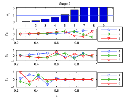
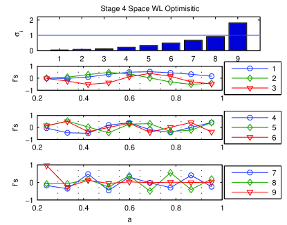
Each data model corresponds to its own Fisher matrix ${\rm\bf F}$ from which the the $\vec{f}_{i}$’s, $\sigma_{i}$’s and the FoM can be calculated. Figure 1 gives the errors $\sigma_{i}$ and modes $\vec{f}_{i}$ corresponding to the DETF “Stage 2” data minus clusters. Stage 2 is the DETF projection of the data upon completion of existing projects. The DETF defines major longer term projects as “Stage 4” and smaller faster future programs as “Stage 3”. Figure 2 gives the same information for a particular Stage 4 data model. None of the DETF data models are powerful enough to constrain all nine directions in our parameter space. This is reflected in large values of $\sigma_{i}$ for larger $i$. We do not trust our formalism to give meaningful answers in directions that place bounds weaker than unity on the $w_{i}$’s, and such weak constraints are not likely to enlighten us about dark energy. We handle this issue by re-setting all $\sigma_{i}>1$ to unity when we calculate the FoM. That way changes in $\sigma_{i}$ in directions where the method is not trusted do not contribute to changes in the FoM.

Figure 2: The impact of the DETF “Stage 4 Space Weak Lensing Optimistic” data model: This is a much higher quality data set vs Stage 2. More modes are well measured and the well measured modes reach to higher redshift (lower $a$). This plot has the same format as Fig. 1

The 9D FoM’s reported here use grids $\{a_{i}\}$ with minimum redshift $z_{min}\equiv 1/(a_{min}-1)=0.01$, $z_{max}=4$ with the grid uniform in $a$. We considered a variety of different grids (varying the spacing pattern, redshift range and total grid points $N_{G}$)EPA . The final grid was chosen to give the highest FoM’s which means we use the parameters which are best measured by the model data sets. Increasing $N_{G}$ beyond the point where the well measured modes are well resolved does not significantly change the FoM’s or the shapes and $\sigma_{i}$’s of the well measured modes. We find this convergence under increasing $N_{G}$ an attractive feature of our parameterization and we found $N_{G}=9$ large enough to achieve convergence.

Independently measured modes of $w(a)$ (the $\vec{f}_{i}$’s) reveal interesting details about each data model. The fact that the best measured Stage 2 $\vec{f}_{i}$’s (shown in Fig. 1) approach zero for $a<0.5$ (larger redshifts) but the corresponding Stage 4 modes (in Fig. 2) do not illustrates the deeper redshift reach of the Stage 4 data. Other specific differences among data models can be understood by inspecting the plots in EPA .

Our form for $w(a)$ has been used previously by others applied to different data modelsHuterer and Turner (2001); Huterer and Starkman (2003); Knox et al. (2004); Linder and Huterer (2005) (see also Riess et al. (2006)). To the extent that comparison is possible our work is consistent with these earlier papers. In particular, the claims in Linder and Huterer (2005) that there are only two measurable $w$ parameters stems from a different formal definition of what it means to measure a parameter usefully. The choice we make here is best suited to our purpose, which is to make a direct comparison with the DETF methods.

There are some small technical differences between our calculations and those in the DETF report. When we use two supernova data models in combination they share the same nuisance parameters (except for the photometric redshifts). The DETF calculations keep the nuisance parameters separate. The PLANCK prior is the same one used by the DETF, but the Fisher matrix is expressed in the variables $\{n_{s},\delta_{\zeta},\omega_{m},\omega_{b},\theta_{s}\}$ where we use $ln(\theta_{s})=-0.252ln(\omega_{m})-0.83ln(\omega_{B})-ln(D_{A}^{co}(a*))+8.2094$ (from Hu (2005)) These parameters are defined in the DETF report. Some other modest differences stem from the shortcomings of the transfer function formalism discussed in section 9.2 of the DETF appendix. These small differences from the DETF calculations are included in all the FoM’s presented here (DETF and 9D) so our comparisons of FoM’s will reflect the different $w$ parameter choices only.

IV Results and Interpretation

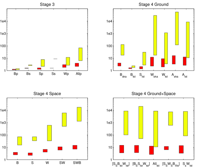
The DETF present their main results in four bar charts showing the FoM ranges for particular data models. The values are given as ratios to the Stage 2 FoM so that progress beyond Stage 2 can be read directly, with increasing progress corresponding to larger values along the y-axis. The four panels in Fig. 3 show equivalent plots (using the same DETF data models minus clusters). The dark bars show the DETF FoM and the light bars show the 9D FoM. The 9D FoM shows much larger values for all the strong data models.

One can see that good combinations of Stage 3 data give 9D FoM improvements of an order of magnitude and strong Stage 4 data combinations give 9D FoM improvements of three orders of magnitude or more. Compared with the DETF results (about half an order of magnitude to Stage 3 and one order of magnitude to Stage 4) this is not only a strong showing overall, but specifically the 9D FoM exhibits a greater improvement factor going from Stage 3 to Stage 4 as compared with the DETF FoM. Given the ballpark costs quoted (but not independently verified) by the DETF of a few $\times\$10^{7}$ for Stage 3 and 0.3-1 $\times\$10^{9}$ for Stage 4, our work indicates that good Stage 4 projects tend to be much more cost effective (about ten times better in $ per FoM increment) than Stage 3 projects. The opposite seems to be the case when using the DETF FoM, but our work shows that this is only because the 2D DETF parametrization prevents the better experiments from showing their full capabilities.

The DETF FoM is constructed in a 2-D parameter space. To build intuition, consider the following effective “reduction to 2-D” of the 9D FoM:

$${\cal F}_{2}\equiv{\cal F}_{9}^{2/D_{e}}$$ (4)

Here ${\cal F}_{2}$ and ${\cal F}_{9}$ are the reduced and regular 9D FoM’s respectively. One can think of ${\cal F}_{2}$ as the product of only two $1/\sigma_{\rm eff}$’s where $\sigma_{\rm eff}$ is a suitably defined geometric mean of the $\sigma_{i}$’s. The “effective dimension” $D_{e}$ can be thought of as the number of directions constrained by the data model in 9D parameter space.

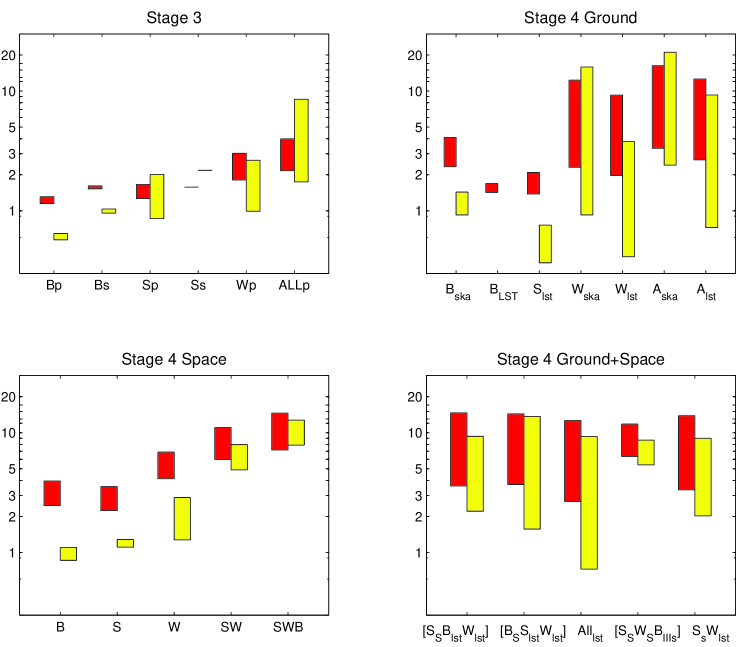
Figure 4 is the same as Fig 3 except Eqn. 4 has been applied to all the 9D FoM’s. Values of $D_{e}$ were assigned to the data models (details in the caption) to create an approximate match (by eye) between rescaled 9D and DETF FoM’s. Inspection of Fig. 4 suggests that the rescaling accounts for may of the differences between the FoM’s. A refined assignment of $D_{e}$’s gradually increasing with improving data models would give an even better account of the differences (but still would not match up every detail). Successful matching of the DETF and 9D FoM’s after rescaling implies that $D_{e}$ directions in the 9D space are measured as well as the two DETF parameters. This applies only in an average sense: The best 9D modes are measured much better than the best DETF parameter, others are less well measured. We present this rescaling to give intuition about the similarities and differences between the DETF and 9D FoM’s. The similarity of the DETF and 9D bars in Fig. 4 help one see how the detailed DETF conclusions about the relative value of different techniques and combinations of techniques are unchanged by our analysis. However, we do not expect Eqn. 4 to offer a universal relationship between the two FoM’s that extrapolates to all possible data models.

Figure 3: Figure of merit improvements vs Stage 2 for DETF data models: Dark bars show the DETF FoM. To the right of each dark bar is a light bar that reflects the 9D FoM for the identical data model. The 9D FoM registers a much greater impact from each data model, and also shows a much greater improvement at Stage 4 vs Stage 3. Each panel corresponds to one of the four main bar charts in the DETF report (B = “Baryon Oscillations”, S = “Supernovae”, W = “Weak Lensing”, A = “All” see pp. 16-20 of Albrecht et al. (2006)).The x-axis labels are similar to those on the DETF plots, but abbreviated.

Figure 4: Rescaled FoM’s: This is identical to Fig. 3 except all the 9D FoM’s have been scaled according to Eqn. 4. We use $D_{e}=2.5$ for Stage 2, $D_{e}=3$ for Stage 3, $D_{e}=4$ for Stage 4 pessimistic and $D_{e}=4.5$ for Stage 4 optimistic. These plots suggest that the scaling gives a reasonable account of the impact of measuring more parameters in 9D vs 2D spaces demonstrated in Fig. 3.

Imposing additional constraints or “priors” on specific parameters generally will improve the figures of merit. The DETF report has a plot similar to Fig. 5 (dark bars) which illustrates the “impact factor” (factor by which the FoM improves) from imposing stronger priors on the curvature and the Hubble constant. The DETF found the impact to be modest, and noted that the best data models actually determine the parameters so well themselves that the impact of additional priors was small.

Figure 5: Impact of adding additional constraints on curvature (left side) and the Hubble constant (right side): Dark bars show the impact on the DETF FoM and light bars show the impact on the 9D FoM. The y-axis is the factor by which the FoM’s change (for Stage 4 space, without stage 2) when the additional constraints are imposed. Changing from the DETF to the 9D parameters does not undermine the insensitivity to additional constraints reported by the DETF. This plot corresponds to the plot on p.14 of Albrecht et al. (2006) (in a different format).

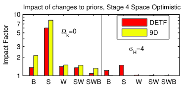
Our work shows that DETF data models can constrain more $w(a)$ parameters than the two considered by the DETF. Does this improvement comes at the expense of poorer constraints on other parameters, due to the greater flexibility of the dark-energy model? The lighter bars in Fig. 5 show the impact factor on the 9D FoM. In no case is the impact substantially greater for the 9D case, indicating that going to the 9D $w(a)$ model does not significantly undermine the constraints on the curvature and Hubble constant from the modeled data. In fact, the 9D impact factors are much smaller with the Hubble prior than for the DETF FoM, suggesting that the directions in the 9D space constrained by these data models have even less degeneracy with the Hubble parameter than $w_{0}$ and $w_{a}$.

V Conclusions

We have analyzed a FoM for dark energy probes which is defined in a nine-dimensional parameter space, up from the (already ambitious) two-parameter space used by the DETF. Our 9D FoM gives a more complete account of the impact of a given data model. We find the DETF data models constrain significantly more parameters than the two used by the DETF, leading to vastly improved FoM’s in the D9 space. Our rescaling law gives an intuitive account of the impact of measuring more parameters.

The 9D FoM follows the same logic as the DETF FoM, namely it attaches equal weight to any constraint on $w(a)$. The measurement of a non-zero value for any of the independently measured combinations $\vec{f}_{i}$ would be equally significant in that it would rule out a pure cosmological constant. Thus the higher values of the 9D FoM (vs the DETF) reflect genuinely greater discovery power.

The effective number of parameters measured ($D_{e}$) increases with the quality of the project, and consequently so does the gap in the impact registered by the 9D vs DETF FoM’s. Good Stage 4 projects measure more than four parameters and produce a three or four order of magnitude improvement in the 9D FoM vs a one order of magnitude improvement in the DETF FoM. As a result, our 9D work indicates that good Stage 4 projects achieve a ten times lower estimated cost per FoM increase than Stage 3 projects, the reverse of the DETF conclusion. Aside from this major difference, the detailed DETF conclusions about the relative value of different techniques and the importance of combining techniques are unchanged by the 9D analysis.