Energy transport, overshoot, and mixing in the atmospheres of M-type main- and pre-main-sequence objects

We constructed hydrodynamical model atmospheres for mid M-type main-, as well as pre-main-sequence (PMS) objects. Despite the complex chemistry encountered in these cool atmospheres a reasonably accurate representation of the radiative transfer is possible, even in the context of time-dependent and three-dimensional models. The models provide detailed information about the morphology of M-type granulation and statistical properties of the convective surface flows. In particular, we determined the efficiency of the convective energy transport, and the efficiency of mixing by convective overshoot. The convective transport efficiency was expressed in terms of an equivalent mixing-length parameter $\alpha_{\mathrm{MLT}}$ in the formulation of mixing-length theory (MLT) given by Mihalas (1978). $\alpha_{\mathrm{MLT}}$ amounts to values around $\approx 2$ for matching the entropy of the deep, adiabatically stratified regions of the convective envelope, and lies between 2.5 and 3.0 for matching the thermal structure of the deep photosphere. For current spectral analysis of PMS objects this implies that MLT models based on $\alpha_{\mathrm{MLT}}=2.0$ overestimate the effective temperature by 100 K and surface gravities by 0.25 dex. The average thermal structure of the formally convectively stable layers is little affected by convective overshoot and wave heating, i.e., stays close to radiative equilibrium conditions. Our models suggest that the rate of mixing by convective overshoot declines exponentially with geometrical distance to the Schwarzschild stability boundary. It increases at given effective temperature with decreasing gravitational acceleration.

1 Introduction

The increasing number of stars, brown dwarfs, and extrasolar planets of spectral class M or later discovered by infrared surveys and radial velocity searches has spawned a great deal of interest in the atmospheric physics of these objects. Their atmospheres are substantially cooler than the solar atmosphere, allowing the formation of molecules, or even liquid and solid condensates. Convection is a ubiquitous phenomenon in these atmospheres shaping their thermal structure and the distribution of chemical species. Hydrodynamical simulations of solar and stellar granulation including a realistic description of radiative transfer have become an increasingly powerful and handy instrument for studying the influence of convective flows on the structure of late-type stellar atmospheres as well as on the formation of their spectra (e.g., Nordlund 1982; Steffen et al. 1989; Chan & Sofia 1989; Nordlund & Dravins 1990; Cattaneo et al. 1991; Ludwig et al. 1994; Gadun & Pikalov 1996; Steiner et al. 1998; Stein & Nordlund 1998; Asplund et al. 1999; Vögler & Schüssler 2003; Robinson et al. 2004). Here we report on efforts to construct hydrodynamical model atmospheres for mid M-type objects. The spectral type just borders the temperature where the formation of condensates becomes important. The motivation of this investigation was twofold: first, pre-main-sequence (PMS) evolutionary models of M-type stars and brown dwarfs based on mixing-length theory (MLT, Böhm-Vitense 1958) to describe the convective energy transport depend sensitively on the poorly constrained mixing-length parameter $\alpha_{\mathrm{MLT}}$ (Baraffe et al. 2002). Our hydrodynamical models represent convection essentially from first principles, and are free of the uncertainties of MLT allowing to put the stellar models on a firmer footing. Second, the distribution of dust clouds in cool brown dwarfs depends on the efficiency of mixing of their atmospheres by convective overshoot (Ackerman & Marley 2001; Allard et al. 2003; Helling et al. 2004). For other work on the modeling of dust cloud formation in very low mass stars and brown dwarfs, see e.g. Cooper et al. (2003) and Tsuji (2005), and references therein. While by construction MLT cannot describe convective overshoot it is naturally represented in our three-dimensional hydrodynamical models.

The present investigation is extending a previous study of an M-dwarf atmosphere by Ludwig et al. (2002, hereafter LAH) to PMS objects at lower surface gravity. A preliminary account of the results was given in Ludwig (2003). We start in Sect. 2 with an overview of the model construction, in particular related to approximations we adopted in the radiative transfer. In Sect. 3 we discuss the general morphology of the convective flows in the M-type atmospheres and present some statistical properties. In Sect. 4 we provide estimates of the efficiency of the convective energy transport in terms of an effective mixing-length parameter, and discuss consequences for the analysis of PMS M-type objects in the framework of present standard model atmospheres. We continue in Sect. 5 by characterizing the properties of the atmospheric mixing found in the hydrodynamical models, and conclude with final remarks in Sect. 6. In our investigation we take repeatedly recourse to the solar atmosphere as standard benchmark.

2 Model overview

Table 1: The RHD models discussed in the paper: ID is the identifier used to refer to a model in this paper, $T_{\mathrm{eff}}$ the effective temperature of the model including an estimate of its RMS fluctuations, $\log g$ the preset gravitational acceleration, Size is the geometrical size of the computational domain (XxYxZ, where Z denotes the vertical, X and Y the horizontal directions), $H_{\mathrm{P}}^{\mathrm{surf}}$ the pressure scale height at the surface, $P_{\mathrm{surf}}$ the pressure at the surface, $v_{\mathrm{rms}}^{\mathrm{max}}$ the maximum vertical RMS velocity in the convective layers, $\delta I_{\mathrm{rms}}/I$ the relative intensity contrast, $\alpha_{\mathrm{MLT}}$ (evo) the mixing-length necessary to match the asymptotic entropy (see Sect. 4), $\alpha_{\mathrm{MLT}}$ (phot) the mixing-length parameter necessary to match the model’s temperature in the deep photosphere, $H_{\mathrm{fex}}$ the scale height of the decline of the atmospheric mixing rate (see Sect. 5), and Modelcode an internal model identifier. Parenthesis indicate uncertain values.

ID	$T_{\mathrm{eff}}$	$\log g$	Size	$H_{\mathrm{P}}^{\mathrm{surf}}$	$P_{\mathrm{surf}}$	$v_{\mathrm{rms}}^{\mathrm{max}}$	$\delta I_{\mathrm{rms}}/I$	$\alpha_{\mathrm{MLT}}$	$\alpha_{\mathrm{MLT}}$	$H_{\mathrm{fex}}$	Modelcode
	[K]		[Mm]	[Mm]	$\log_{10}$	[ m s-1]	[%]	(evo)	(phot)	[$H_{\mathrm{P}}$]
C5	$2789\pm 0.7$	5.0	0.25x0.25x0.087	0.012	6.1	240	1.2	(1.5)	(2.5)	0.5	d3gt30g50n18
C4	$2800\pm 1$	4.0	3.75x3.75x1.16	0.13	5.3	450	3.0	2.1	2.5	3.2	d3gt30g40n1
C3	$2800\pm 2.7$	3.0	37.5x37.5x13.8	1.5	4.5	820	8.2	2.1	2.8	(18)	d3gt30g30n1
H4	$3280\pm 2.8$	4.0	4.38x4.38x1.54	0.19	5.2	690	5.4	1.85	3.0	(28)	d3gt33g40n1
HX	$3275\pm 2.8$	4.0	4.38x4.38x1.81	0.19	5.2	690	5.6	-	-	-	d3gt33g40n2
S	$5640\pm 14$	4.44	6.0x6.0x3.2	0.15	5.1	2600	16	-	-	2.4	sun3d
SG	$4610\pm 23$	2.94	141x141x95.3	3.8	4.4	3400	21	-	-	-	d3gt45g29n1

Figure 1 illustrates the positions of our hydrodynamical model atmospheres in the $T_{\mathrm{eff}}$-$\log g$-plane: three M-type models are located close to $T_{\mathrm{eff}}=2800\mbox{\rm\,K}$ with $\log g$=3.0, 4.0, and 5.0 which form a $\log g$-sequence. In the following we shall refer to them as models C3, C4, and C5, respectively. To assess temperature effects, a 500 K hotter M-type model was constructed at $T_{\mathrm{eff}}$=3280 K and $\log g$=4.0. For further comparison we also considered a solar (in terms of its hydrodynamical properties) model S at $T_{\mathrm{eff}}$=5640 K, $\log g$=4.44, and a model SG of a subgiant at 4610 K and $\log g$=2.94.

For investigating the influence of the position of the upper boundary condition we constructed an additional model HX with the same atmospheric parameters as model H4 but extending 270 km (corresponding to 3.7 $H_{\mathrm{P}}$) higher up than model H4. The flow in the extended region exhibits larger fluctuations than encountered in deeper layers favoring the formation of sharp flow features. For reasons of numerical stability we had to increase the numerical viscosity so that the model is not fully differentially comparable to model H4. Nevertheless, it should give an indication of the level of the influence of the upper boundary, in particular when the upper boundary is located close to the convectively unstable region. In plots that follow, we depict model HX always as triple-dot-dashed line without labeling it by its name like the other models. Naturally, the behavior of model HX closely follows model H4 in the deeper layers so that its connection to model H4 is readily apparent.

All models were evolved until a thermally and dynamically relaxed state was reached. All models except HX have 125x125x82 grid points (XxYxZ direction), HX has 125x125x102 grid points due its larger vertical extent. The numerical grid is equidistant in x- and y- direction while in vertical z-direction the grid spacing is to first order chosen to provide the same number of grid points per pressure scale height. In addition, the resolution is increased in layers around continuum optical depth unity if a steep vertical temperature gradient is present. All models have solar chemical composition. Table 1 summarizes their properties.

Figure 1: The radiation-hydrodynamics models in the effective temperature-gravity plane (cubes). The models are labeled by their IDs used for reference in this paper. The approximate spectral class is indicated at the temperature axis.

The overall methodology applied in this work is the same as in LAH, and we refer the reader to this paper for details beyond the short description we provide here.

The radiation-hydrodynamics (RHD) simulations were performed with a convection code developed by Å.  Nordlund and. R.F. Stein (see Stein & Nordlund 1998, and references therein). The code solves the hydrodynamical equations of compressible gas dynamics coupled with non-local radiative transfer in three spatial dimensions. The time-independent radiative transfer is treated assuming strict LTE. The wavelength dependence of the radiation field is represented by a small number of wavelength bins. Open lower and upper boundaries, as well as periodic lateral boundaries are assumed. The effective temperature of a model (i.e., the average emergent radiative flux) is controlled indirectly by prescribing the entropy of inflowing material at the lower boundary. Magnetic fields and rotation are neglected. Opacities and equation-of-state have been adapted to the conditions encountered in M-type atmospheres. The equation of state includes the ionization of H and He , as well as $\mathrm{H}_{2}$ molecule formation according to Saha-Boltzmann statistics. $\mathrm{H}_{2}$ molecule formation is the thermodynamically most important process in the M-type atmospheres. The opacities include contributions of molecular lines but neglect contributions of dust grains which is a good approximation at the temperatures prevailing in the models. The opacities were extracted from the opacity data base of the PHOENIX model atmosphere code (for a description of PHOENIX and corresponding opacities see Hauschildt et al. 1999; Ferguson et al. 2005).

2.1 Radiative transfer

We want to derive quantitative estimates of the mixing by convective overshoot, as well as obtain a measure of the efficiency of the convective energy transport. For addressing these issues, the RHD models have to give a reasonably accurate representation of the actual atmospheric conditions. Here we are particularly concerned about the radiative energy transport, which is complicated by the huge number of molecular absorption lines. In our RHD models, we use a multigroup technique (dubbed Opacity Binning Method, hereafter OBM) for modeling the radiative energy exchange which employs four groups for representing the wavelength dependence of the radiation field (Nordlund 1982; Ludwig 1992; Ludwig et al. 1994; Vögler et al. 2004, LAH). The wavelength groups have been optimized for an atmosphere at $T_{\mathrm{eff}}$=2900 K and $\log g$=5.3. Figure 2 illustrates the accuracy which is achieved with the OBM for the present models. We compare 1D MLT model structures ($\alpha_{\mathrm{MLT}}$=1.0) in radiative-convective equilibrium computed with the OBM approximation and high-precision opacity sampling. While there are differences between the atmospheric structures, the OBM nevertheless provides a significant improvement with respect to a simple grey approximation. Temperature differences get larger as one moves away from the atmospheric parameters the OBM was optimized for, and reach up to 250 K in the model at 2800 K and $\log g$=3.0. However, in the present context it is not so much the absolute temperature error as the change of the temperature gradient which is relevant.

Convection is driven by buoyancy forces whose dynamical effects scale with the entropy gradient. The thermal structure is controlled by a balance between radiative and advective (due to compression or expansion of mass elements) heating (or cooling) of which the Péclet number (see appendix A for its definition and computation) is a convenient dimensionless measure. In the deeper photospheric layers, the OBM profiles shown in Fig. 2 have steeper temperature gradients than the profiles based on opacity sampling. For a given velocity, this makes the rate of temperature change of a mass element moving in vertical direction larger. In other words, the time scale of advection related temperature changes becomes shorter, and the Péclet number larger as long as the radiative time scales remain the same. The opposite behavior is present in the higher photospheric layers. The typical Péclet numbers turn out to be by a factor of 1.2 times larger for the $\log g$=5.0, and by up to a factor of 2 times smaller for the $\log g$=3.0 model comparing OBM to the opacity sampling stratifications.

Figure 2: Comparison of the pressure-temperature structure between 1D hydrostatic model atmospheres in radiative-convective equilibrium based on the OBM (solid lines) with four wavelength groups, and PHOENIX models based on direct opacity sampling employing several $10^{4}$ wavelength points (dash-dotted). Shown are two examples at $T_{\mathrm{eff}}$=2800 K, $\log g$=3.0 and 5.0, respectively. For clarity, the $\log g$=3.0 models were shifted by +1000 K. Also shown is a model employing grey radiative transfer (dotted line). The pressure is given in units of the pressure at Rosseland optical depth unity $P_{\mathrm{surf}}$.

To mitigate the effects of the shortcomings, primarily related to the OBM approximation in the radiative transfer, we took a differential approach when measuring model properties: whenever possible we compared RHD and hydrostatic model atmospheres based on the same OBM radiative transfer scheme since we were interested to study the systematic change of model properties with effective temperature and gravitational acceleration. However, there remains the possibility that even this differential approach cannot fully eliminate the impact of the artificial shift of the Péclet number introduced by the OBM approximation among the models. This has to be kept in mind when interpreting results later.

3 Morphology of granulation in M-type objects

Figure 3 shows an inter-comparison of the granulation patterns typically encountered during the temporal evolution of our RHD models. The first thing to note is that surface convection in M-type objects produces a granular pattern qualitatively resembling solar-type granulation: bright extended regions of up-welling material which are surrounded by dark concentrated lanes of down-flowing material. The dark lanes form an interconnected network. Looking more closely, however, granules are less regularly delineated in M-type objects. The inter-granular lanes show a higher degree of variability in terms of their strength – in particular in comparison to the solar model S, to lesser extend in comparison to the subgiant model SG. A feature which is uncommon in the solar granulation pattern are the dark “knots” found in or attached to the inter-granular lanes prominent in the M-type models C5 and C4. The knots are associated with strong downdrafts which carry a significant vertical component of angular momentum.

We have no convincing explanation at hand why convective flows in M-type atmospheres tend to form such vortical structures. It is unlikely that they are (as suspected by the referee) an artifact related to the boundary condition since the structures do not reach up into layers close to it. Moreover, the test model HX shows also the knots despite the fact that its upper boundary is located about 10 $H_{\mathrm{P}}$ above the continuum forming layers. The presence or absence of knots may rather be related to the level of horizontal shearing in the layers around optical depth unity where convective driving is usually strongest and is important for the formation of flow structures. Figure 7 illustrates that under solar-like conditions (models S and SG) shear flows are common in the surface layers, and are much more pronounced than in the M-type atmospheres. Such shear flows make the formation of structures extending in vertical direction difficult, and may be the reason why the knots do not appear in the solar-like models and are less developed in models H4 and C3.

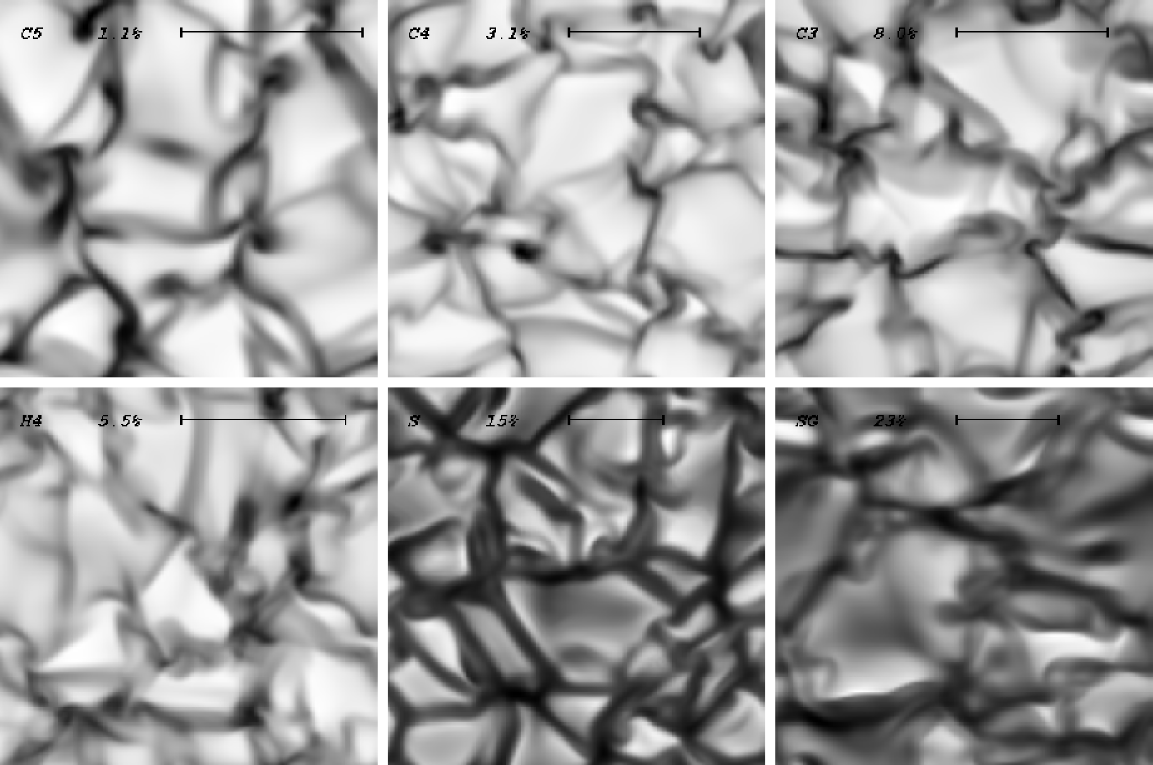
Figure 3: Granulation patterns of the six RHD models. The model IDs are given in the upper left corners (see Tab. 1) of the images. Shown are snapshots of the emergent intensity in the continuum. For each image a separate grey scale is used, lighter shades correspond to higher intensities. The relative intensity contrast of the particular image is stated, and the bar indicates a length of $10\times H_{\mathrm{P}}^{\mathrm{surf}}$.

As a side-point we would like to remark that it is not immediately clear why the knots appear in fact dark. However, centrifugal forces in the vortices are evidently not strong enough to lead to an evacuation of their interior on a level that would allow radiation from deeper, hotter layers to escape and let them appear brighter than their surroundings. The conditions are not as extreme as for bright flux tubes in the solar photosphere where magnetic pressure allows for a substantial degree of evacuation.

The width of the inter-granular lanes relative to the typical granular size is smaller in our M-type objects of higher gravity. Inspecting the velocity field (not shown) in vicinity of the continuum forming layers shows less pronounced size differences. This indicates that the relatively broader lanes in the solar case are the result of a stronger smoothing of the temperature field due to a more intense radiative energy exchange, i.e., the effectively smaller Péclet number of the flow around optical depth unity in the hotter objects. Figure 4 shows an overview of the mean T-$\tau$ (the temperature was averaged over time and surfaces of equal optical depth) relations found in the RHD models. One recognizes that in the M-type objects the thermal structure is influenced by convection to much lower optical depths than in the solar-type stars.

The temperature model HX is on the scale of the plot identical to model H4 in deeper layers but shows a noticeable deviation at low optical depth close to the upper limit over which the stratifications have been averaged. While perhaps not surprising considering the different placement of its upper boundary, the difference may be in part traced back to the different viscosity which damps the velocity field and leads to less convective heating in the atmospheric layers which are convectively unstable (see Sect. 4 for a discussion of the interplay of convection and radiation in the atmospheric layers).

Figure 4: Mean temperature (averaged over time and surfaces of constant optical depth) relative to effective temperature for the RHD models as function of Rosseland optical depth. For clarity the curves are shifted by $\{1,2,3,4,5\}\times 0.05$ for the models C4, C3, H4/HX, S, and SG, respectively.

3.1 Horizontal scales

Primarily due to the variation of the gravitational acceleration (by a factor of 100) the convective cells in our models span a substantial range in geometrical size. However, taking the pressure scale height at optical depth unity $H_{\mathrm{P}}^{\mathrm{surf}}$ as reference the variation is largely reduced. The bars in Fig. 3 are placed to suggest that the horizontal size of the cells indeed roughly scales with $H_{\mathrm{P}}^{\mathrm{surf}}$. This is quantified in Fig. 5 for the intensity pattern and Fig. 6 for the pattern of the vertical velocity. The maximum power in the spectra of the intensity pattern of the M-type objects lies between 5 and 8 $H_{\mathrm{P}}^{\mathrm{surf}}$, the maximum power of the velocity pattern between 3 and 6 $H_{\mathrm{P}}^{\mathrm{surf}}$. In both cases the spectra of the solar-type objects are slightly but noticeable shifted towards smaller wavenumbers (larger spatial scales). While the relation between M-type and solar-type objects is the same in both diagnostic variables, it came as a surprise – at least to the authors – that both variables do not provide the same value for the typical cell size. The different slopes in the intensity and velocity spectra towards larger scales might be related to this finding. If one considers a pure random pattern of a given characteristic scale, a slope of unity (in the chosen representation of power) is to be expected towards larger scales. In this case the signal at large scales is the result of a mere random superposition of residual contributions from smaller scale features. The intensity spectra follow this random model quite closely while the velocity spectra show noticeably larger deviations with steeper slopes. We do not have an explanation at hand. However, considering the range of stellar parameters covered by our models, the shape of spectra show a large degree of similarity. In particular, the typical granular scales (in intensity) turn out to be the same within a factor of two lying between 5 and 10 $H_{\mathrm{P}}^{\mathrm{surf}}$for all objects.

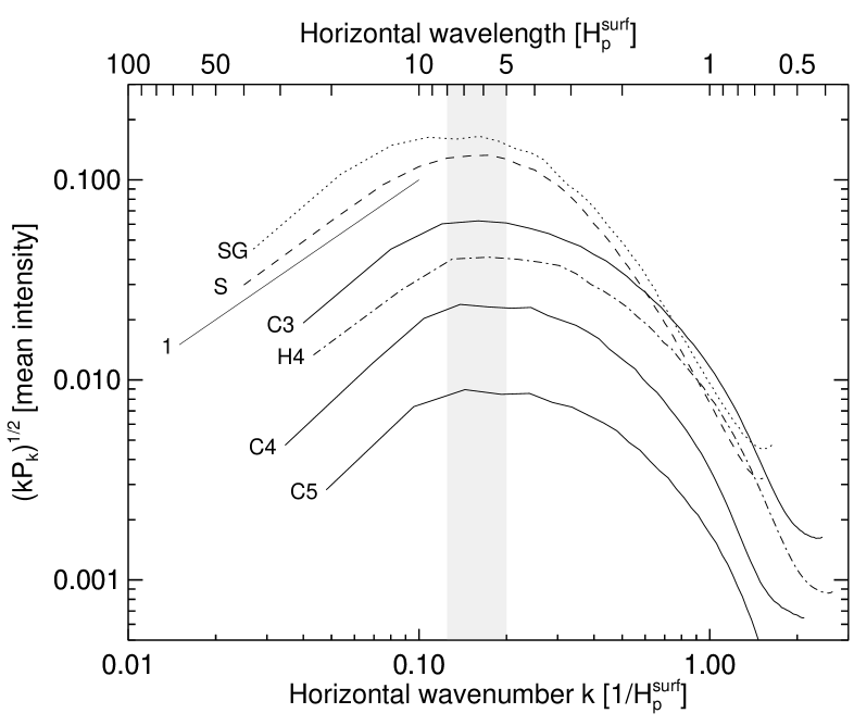
Figure 5: Spatial power spectra of the emergent intensity as a function of horizontal wavenumber $k$. The amplitude power is given in units of the temporally and horizontally averaged intensity. The curves are labeled with the IDs of the models (see Tab. 1), the curve labeled “1” indicates a power-law with slope unity. The grey stripe indicates the range of horizontal scales within which the power maxima of the M-type models are located.

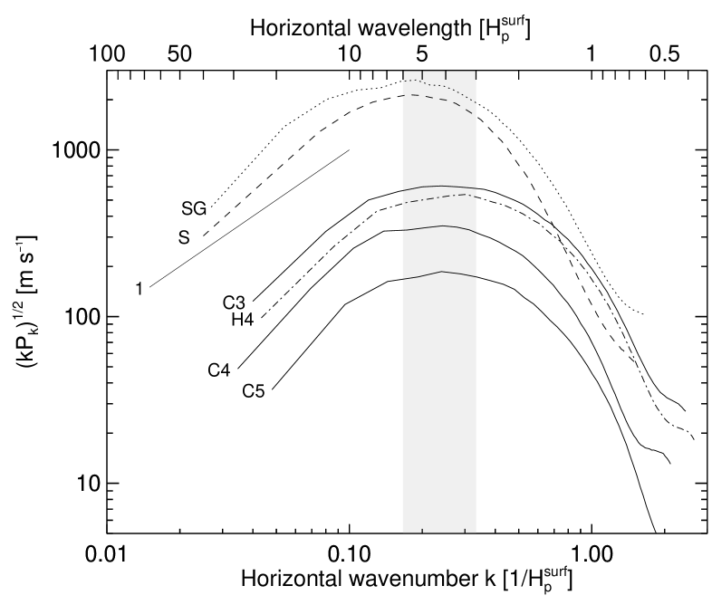
Figure 6: Spatial power spectra of the vertical velocity as a function of horizontal wavenumber $k$. The velocities are taken from the layer where the convective velocities reach their maxima. The curves are labeled with the IDs of the models (see Tab. 1), the curve labeled “1” indicates a power-law with a slope of one. The grey stripe indicates the range of horizontal scales within which the power maxima of the M-type models are located.

3.2 Velocities and turbulent pressure

Figures 7 and 8 show the run of the root-mean-square (RMS) vertical as well as horizontal velocity component, and of the turbulent pressure, respectively. The averages were taken over time and fixed geometrical height. As is evident from the figures, the vertical velocity and turbulent pressure follow each other rather closely. In the higher atmospheric layers, the velocity field – especially in the models with more vigorous convection – is dominated by horizontal motions. Test model HX closely follows model H4 in the deeper layers but shows reduced amplitudes in the higher layers. As indicated previously we interpret this as primarily a consequence of the increased numerical viscosity in model HX, and not so much due to the larger extend of the model. Generally, the velocities are smaller in the M-type objects then in the solar-like objects. Due to their substantially lower $T_{\mathrm{eff}}$ in comparison to the solar-type models, the requirement to transport the nominal energy flux is already met by convection at lower velocities in the M-type models, leading to the overall lower “hydrodynamic activity” in these objects.

Figure 7: Root-mean-square velocities for the RHD models as a function of gas pressure relative to the individual surface pressures $P_{\mathrm{surf}}$ (see Tab. 1). Black lines depict the vertical, grey lines the horizontal velocity component.

Figure 8: Turbulent pressure $\left\langle\rho v_{z}v_{z}\right\rangle$ as a function of gas pressure relative to the individual surface pressures. The turbulent pressure quite closely follows the vertical velocity as depicted in Fig. 7.

3.3 Horizontal fluctuations

Figures 9 and 10 show the relative spatial and temporal RMS fluctuations of temperature and pressure at given geometrical height. In the M-type models the temperature fluctuations stay at a very modest level nowhere exceeding 4 % – even including model HX. In the optically thin layers, model C4 shows systematically larger temperature fluctuations than model H4 of higher $T_{\mathrm{eff}}$ but of the same surface gravity. This is an imprint of the reduced capacity of the radiation field in model C4 to smooth horizontal temperature differences. The pressure fluctuations reach larger values than the temperature fluctuations, and show a systematic increase with height. Note that in our dwarf model C5, the pressure fluctuations only reach a very modest level of about 4 %. From this we expect that in cooler, dust-forming main-sequence objects, thermodynamic fluctuations are even smaller so that dust formation conditions vary little in a given layer. Model HX shows a rapid increase of fluctuations with height which is typically found when the flow field is dominated by wave motions. The correspondence to model H4 in the overlapping region is quite good indicating that fluctuations in temperature and pressure are little affected by the location of the upper boundary.

Figure 9: Relative RMS temperature fluctuations in horizontal planes as a function of gas pressure relative to the individual surface pressures $P_{\mathrm{surf}}$ (see Tab. 1). The clipped maxima in the curves for models S and SG reach 0.23 and 0.30, respectively.

Figure 10: Relative RMS fluctuations in horizontal planes as a function of gas pressure relative to the individual surface pressures.

3.4 Spatial correlation of vertical velocity and entropy

In this section, we want to give an overview of some two-point correlations found in our models. The width of two-point correlations in vertical direction has been considered as measure of the mean-free-path of mass elements entering MLT – the mixing-length $\Lambda$, and as such has been the target of many investigations. The (linear) correlation coefficient of a quantity $x$ between two layers located at heights $z_{1}$ and $z_{2}$ is given by

$${\mathrm{C}\left[x_{1},x_{2}\right]}=\frac{\left\langle x_{1}x_{2}\right\rangle-\left\langle x_{1}\right\rangle\left\langle x_{2}\right\rangle}{{\sigma_{x_{1}}}{\sigma_{x_{2}}}}$$ (1)

where $\sigma_{x_{i}}$ is the standard deviation of $x$ at height $z_{i}$, and the angular brackets denote the average over time and horizontal position. In a seminal paper, Chan & Sofia (1987) found in hydrodynamical models of stratified efficient convection that the full-width-at-half-maximum (FWHM) of the correlation function of the vertical velocity, as well as temperature, scaled with the pressure scale height and not density scale height. In a follow-up study, Chan & Sofia (1989) showed that the result is robust against variations of the ratio of the specific heats $\gamma$ of the gas. Singh & Chan (1993) found that the width of correlation changes moderately with Prandtl number. Kim et al. (1995) studied the case of inefficient convection in the Sun. Their model included radiative transfer effects (in diffusion approximation) as well as effects of the ionization of hydrogen and helium. Under the conditions studied by Kim and collaborators, the width of the correlation function of the velocity scaled with pressure and density scale height, while the width of the temperature correlation with neither of both. Kim et al. had to restrict their investigation to optically thick regions. Robinson et al. (2003, 2004) included also optically thin layers in their hydrodynamical models of the Sun and a subgiant star (at $T_{\mathrm{eff}}$=4990 K, $\log g$=3.37). The radiative transfer was treated in grey Eddington approximation. Robinson and collaborators found a complex height-dependence of the width of the correlation of the vertical velocity and entropy fluctuations. Especially the last result shows that we cannot expect to find a universal behavior of the correlations in stratified convection under all possible circumstances – in particular, in the case of inefficient convection which is most important for stellar structure models. However, there might be still hope to find general trends which may serve as buildings blocks for an improved treatment of convection beyond MLT.

Figures 11 and 12 provide an overview of the velocity and entropy correlations found in our models. Our models contribute to the ongoing discussion in a twofold way: they cover a large range of stellar parameters and include an elaborate treatment of the radiative transfer in the optically thin layers. The overall behavior of the correlations is complex, but some general features can be identified: i) considering that the models cover about a factor of two in $T_{\mathrm{eff}}$ and one hundred in $\log g$, a certain uniformity in the width of the distributions in the convection dominated layers is apparent; ii) in the sub-photospheric layers the entropy correlation is more peaked than the velocity correlation; iii) with the exception of model C5 the velocity correlation become broader in radiation dominated layers; iv) the widths of the correlations tend to shrink with increasing depth, possibly towards an asymptotic limit (different for velocity and entropy) – in line with the findings of Chan & Sofia (1989); v) the width of the entropy correlation of the solar model S and subgiant SG passes through a pronounced minimum around optical depth unity; this is accompanied by anti-correlations signifying the thermal behavior of overshooting motions; vi) the degree of uniformity of the correlations is not improved if plotted on the density scale.

The limiting width of the correlation functions is fairly well defined and given in the panels of Figs. 11 and 12. The width of the velocity correlation lies in the same range as values of the mixing-length parameter associated with certain model features which we are going to discuss later. However, one must keep in mind that the width of the correlations varies substantially – sometimes even dramatically – in the models, and that the widths are different for different quantities. In our opinion, a direct association of a width of a correlation with a mixing-length parameter is an over-simplification of the actual situation.

Figure 11: Contour plots of the two-point spatial correlation functions of the vertical velocity (left panels), and entropy (right panels) for the models C3, C4, and C5. The pressure relative to the surface pressure of the two involved height levels (cf. Eq. (1)) are given on abscissa and ordinate. The height coordinates are interchangeable due to the symmetry of the correlation function. The number in the lower right corner of each panel gives the FWHM of the correlation (in units of the local pressure scale height $H_{\mathrm{P}}$) in vicinity of the lower boundary of the computational domain. Contour lines are given for values of $\{-0.5,-0.25,-0.125,0.125,0.25,0.5\}$. Lines with positive contour values are depicted by solid lines, negative ones by dashed lines. Dotted lines are for orientation and have a distance of $\Delta\ln(P/P_{\mathrm{surf}})=1$. The central dotted line coincides with the maximum of the correlation function which is normalized to one.

Figure 12: Same as Fig. 11 for models SG, S, and H4.

4 Convective energy transport

Convection is an important energy transport mechanism in M-type stars. In standard model atmospheres it is treated in the framework of MLT. In this section, we want to address the question whether the simplistic MLT is actually capable to provide a sufficiently accurate description of the convective energy transport under conditions encountered in M-type atmospheres. Figure 13 shows a comparison of the entropy structure of the RHD model atmospheres and standard 1D hydrostatic models in radiative-convective equilibrium assuming different mixing-length parameters. Figure 14 depicts corresponding temperature profiles which allow to approximately translate entropy differences among the profiles in Fig. 13 to temperature differences.

To calculate the entropy profiles of the RHD models, they have been averaged temporally and horizontally on surfaces of constant optical depth. This procedure ensures a particularly good preservation of the energy transport properties of the RHD models (Steffen et al. 1995). Moreover, it reduces the “smearing” of vertical gradients by plane-parallel oscillations which occurs when averaging over fixed horizontal planes. Besides the mixing-length parameter itself, MLT contains a number of further “hidden” parameters intrinsic to the specific formulation of MLT which was chosen. We emphasize that a well-defined calibration of the mixing-length parameter must always be given with reference to the specific formulation in operation. Here, we are using the formulation given by Mihalas (1978). See Ludwig et al. (1999) for details of the implementation.

As already remarked earlier, Fig. 13 illustrates that the sensitivity of the structure of the standard models to the mixing-length parameter increases with decreasing gravity as well as increasing $T_{\mathrm{eff}}$. Model C3 shows a sensitivity of the entropy in the deep, adiabatic layers which is comparable to the sensitivity of solar MLT models. Figure 13 also illustrates that the convectively unstable layers (with entropy gradient $\frac{ds}{d\tau}>0$) extend to small – spectroscopically important – optical depths. M-type atmospheres offer the opportunity to study convection under optically thin conditions.

Figure 13: Entropy as a function of Rosseland optical depth of the RHD models (thick solid lines) in comparison to standard mixing-length models (thin solid lines). For each RHD model three MLT models are plotted with $\alpha_{\mathrm{MLT}}$=1.5, 2.0, and 2.5. The entropy of the MLT models behaves monotonically with $\alpha_{\mathrm{MLT}}$, the $\alpha_{\mathrm{MLT}}$=1.5 model having the lowest entropy in the optically thin, and the highest in the optically thick layers. Model H4 has been offset by $+0.2$ entropy units for clarity, and one special MLT model with $\alpha_{\mathrm{MLT}}$=2.0 has been added (dashed-dotted line; see text). The dashed lines depict the value of entropy present in the adiabatically stratified regions of the convective envelope. Numbers indicate mixing-length parameters necessary to match the RHD structure by MLT models.

Figure 14: Temperature as a function of Rosseland optical depth of the RHD models (thick solid lines) in comparison to standard mixing-length models (thin solid lines). The MLT models are calculated assuming $\alpha_{\mathrm{MLT}}$=1.5. For model H4 a special MLT model with $\alpha_{\mathrm{MLT}}$=2.0 has been added (dashed-dotted line; see text). For clarity, models C4, C3, and H4 have been offset by 500, 1000, and 1500 K, respectively.

The general role of convection can be described as follows: in the convectively unstable layers – here comprising also parts of the optically thin layers – the thermal structure is the result of a competition between adiabatic heating and radiative cooling because a temperature structure in adiabatic equilibrium would be hotter than in radiative equilibrium. The mixing-length model (with $\alpha_{\mathrm{MLT}}=2.0$) depicted by the dashed-dotted line for case H4 is intended to illustrate this (see Figs. 13, 14, and 17): in this model we artificially switched off the convective motions in the layers with $\log\tau_{\mathrm{ross}}\leq-1$. This suppresses the convective heating and forces the temperature to adjust to radiative equilibrium conditions. As evident from the figures, this leads to a substantial drop of entropy and temperature. In the convectively stable layers (with entropy gradient $\frac{ds}{d\tau}<0$) the situation is reversed, and the temperature is controlled by a balance between adiabatic cooling and radiative heating – as far as the RHD models are concerned. The situation is different for the MLT models where by construction no convective (overshooting) motions take place in the formally stable layers, and the temperature is determined by the condition of radiative equilibrium alone.

For decreasing $\log g$ at given $T_{\mathrm{eff}}$, the models tend to stay closer to radiative equilibrium conditions in the optically thin layers. Two factors reduce the efficiency of the convective energy transport: first, Fig. 15 shows that the opacity does not vary radically among the M-type models. Hence, lower gravity models exhibit lower densities at given optical depth, which reduces the thermal energy that can be transported per unit volume, rendering the convective transport of heat more difficult. Second, the pressure scale height increases with decreasing gravity while typical convective velocities increase only modestly. This increases the time scale over which vertically traveling mass elements change their temperature due to adiabatic expansion or compression. The radiative time scale in the optically thin regions, on the other hand, is independent of the spatial scales and mass density which again leads to a shift of the thermal balance towards radiative equilibrium conditions.

As evident from Fig. 16, the pressure-temperature dependence of the adiabatic gradient counter-acts the trend towards radiative equilibrium conditions in our M-type models of lower gravity. In models C3 and H4, the adiabatic gradient is close to its minimum favoring convection due to the formation of H₂ molecules. Nevertheless, the appreciable sensitivity of the MLT models to the mixing-length parameter at lower gravities indicates that convection and radiation operate with comparable efficiency.

Figure 15: Average pressure-temperature profiles of the RHD models (thick lines) overlayed on contours (thin lines) of the ($\log_{10}$) Rosseland mean opacity.

Figure 16: Average pressure-temperature profiles of the RHD models (thick lines) overlayed on contours (thin lines) of the adiabatic gradient.

In Figs. 13 and 14 we compare groups of models of the same $T_{\mathrm{eff}}$ and $\log g$, and consequently the models in each group are constrained to similar temperatures and entropies in vicinity of optical depth unity. Since the entropy- as well as temperature-gradient at this location depend on the mixing-length parameter, this leads to the crossing of the various profiles around $\tau_{\mathrm{ross}}=1$. Deviations from this behavior – in particular shown by the RHD models – come about by residual differential changes of the opacities and thermodynamic properties of the matter among the models. In the case of the RHD models, horizontal fluctuations together with non-linearities in the material functions add to the deviations.

Figure 13 shows that irrespective of the choice of the mixing-length parameter $\alpha_{\mathrm{MLT}}$, no MLT model is capable to match the whole average thermal profile of a hydrodynamical model – at least within the framework of the MLT formulation adopted here. We nevertheless give estimates of the mixing-length parameter matching certain features of the hydrodynamical structure. Multi-dimensional hydrodynamical convection models provide the value of the entropy asymptotically reached in the deep, adiabatically stratified layers of the convective envelope, since it is identical to the entropy of upflowing material in the deepest regions of the hydrodynamical model (for a discussion of the scenario underlying this notion see Steffen (1993), and Ludwig et al. (1999)). We find a mixing-length parameter of 1.5, 2.1, 2.1, and 1.85 for models C5, C4, C3, and H4, respectively, to match the asymptotic entropy. This $\alpha_{\mathrm{MLT}}$ is most relevant for stellar structure models since the asymptotic entropy has a large influence on the radius of a convective stellar object. The value for model C5 (1.5) is highly uncertain since the sensitivity to $\alpha_{\mathrm{MLT}}$ is very small – however, its precise value is also not particularly important since the asymptotic adiabat hardly depends on $\alpha_{\mathrm{MLT}}$. Attributing little weight to model C5, we find that the typical $\alpha_{\mathrm{MLT}}$ suitable for evolutionary models lies around $\approx 2$ for mid to late M-type atmospheres. This value is not very different from the value found for the Sun ($\approx 1.8$), but we do not consider this as an indication of an universal value for $\alpha_{\mathrm{MLT}}$ as was already discussed in LAH.

Now we turn to the optically thin parts of the atmosphere relevant for spectroscopy. We find that mixing-length parameters for matching the temperature in the range $-2\leq\log\tau_{\mathrm{ross}}\leq-1$ of 2.5, 2.5, 2.8, and 3.0, for models C5, C4, C3, and H4, respectively. This range in optical depth was chosen as representative of the deeper photosphere. However, the match in this part does not imply a match over the whole optically thin region. Again, the value for model C5 is uncertain, but not particularly important. All in all we obtain a range of $\alpha_{\mathrm{MLT}}=2.5\ldots 3.0$ when matching the thermal profile of the RHD models. The temperature structure of the hydrodynamical models in the uppermost, convectively stable part of the atmosphere does not deviate much from radiative equilibrium profiles judging by extrapolating from the available MLT models. This indicates that cooling by convective overshoot or heating by waves is not very efficient in the layers immediately adjacent to the surface convective zone.

Model H4 is an exception from the general trend since it becomes convectively stable much earlier than one might expect from extrapolating the MLT models. The exceptional behavior is due to the fact that in this model the adiabatic gradient changes very little along the profile in the upper photosphere (see Fig. 16). The same holds for the actual temperature gradient in the convectively unstable part, making the exact location of the transition from convective instability to stability very sensitive to the actual run of the temperature. Here, we have an example where second order effects can enhance differences to MLT models. Nonetheless, overshooting and wave heating, again, show little impact on the temperature gradient in the (not very extended) stable zone.

A comparison of models H4 and HX in Fig. 13 reveals that the modest temperature differences in the optically thin layers displayed in Fig. 14 correspond to a sizable entropy difference which corresponds to a decrease of the mixing-length parameter of about 0.5 relative to model H4. Such a change would bring the atmospheric value of the mixing-length parameter of model H4 closer to the other M-type models. As argued before the change in the thermal structure of model HX can only be partially attributed to a systematic influence of the upper boundary condition. Nevertheless, taking the change as an estimate of the uncertainty of the derived atmospheric mixing-length parameter, one would still find a rather high value of the mixing-length parameter for model H4 of at least 2.5. The mixing-parameter for matching the asymptotic entropy remains the same between models H4 and HX.

In LAH we discussed the mixing-length parameter necessary to match the maximum vertical RMS velocity of the hydrodynamical model C5 and found a value of 3.5. While we do not perform a similar matching here, Fig. 17 clearly shows that for all RHD models a value substantially larger than 2.5 – including model HX – is necessary to match the maximum velocity.

Figure 17: RMS vertical velocity component of the RHD models (thick solid lines) in comparison to convective velocities from MLT models with $\alpha_{\mathrm{MLT}}$=1.5, 2.0, and 2.5 (thin solid lines) as a function of optical depth. The velocities from MLT increase in the optically thin layers monotonically with increasing $\alpha_{\mathrm{MLT}}$. For model H4 a special MLT model with $\alpha_{\mathrm{MLT}}$=2.0 has been added (dash-dotted line; see text). Models C4, C3, and H4 have been shifted by 500, 1000, and 2000 m s^-1, respectively. The downturn of the velocity in models C4, C3, and H4 at largest optical depth is an artifact of the averaging procedure and should be ignored.

Comparing the overall situation that we encounter in M-type objects to stars of roughly solar effective temperature (and of solar composition) we find that the transition from convectively to radiatively dominated energy transport happens more gradually in M-type objects. This is ultimately linked to the different temperature sensitivity of the dominant opacity (H and H^- bound-free and free-free absorption versus TiO and H₂O molecular line plus H^- bound-free and free-free absorption), and dominant thermodynamic process (H recombination versus H₂ molecular formation) encountered in the two regimes of effective temperature. The values of $\alpha_{\mathrm{MLT}}$ we obtained here when matching the asymptotic entropy are not too different from the values obtained for solar-type stars. However, in solar-type stars a calibrated MLT model merely provides the correct entropy jump. The actual run of the entropy in the optically thick layers is not very well matched: usually, a RHD model predicts a more rapid switching between adiabatically and radiatively stratified layers. In M-type objects, a calibrated MLT model matches the actual thermal profile in the optically thick regions more closely. This property is likely related to the more gradual transition between the two modes of energy transport.

4.1 Spectroscopic effects

In this section, we want to demonstrate which impact the differences between the thermal structures of RHD and MLT models have on spectral properties. Mohanty et al. (2004) used molecular bands of titanium-oxide and lines of neutral atomic alkalis to determine the effective temperatures and surface gravities of M-type PMS objects by comparing synthetic and observed spectra. The temperatures and gravities of the objects studied by Mohanty and collaborators fell into the regime considered here. The authors emphasized that the strengths of the investigated TiO band heads serve as excellent and important temperature indicator. Figures 18 and 19 show two prime spectral regions (wavelengths are given as wavelengths in air) considered in the analysis by Mohanty et al. . For our comparison, we picked case C3 where we found significant differences in the thermal structures between RHD and MLT models. Spectral synthesis calculations were performed with the PHOENIX code on the prescribed structures at a spectral resolution of 0.01 Å. In Figs. 18 and 19 the spectral resolution has been degraded to $\sim 30\,000$ similar to the one in the work of Mohanty et al. .

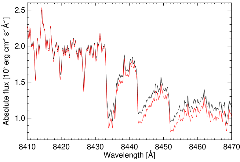
Figure 18: Comparison of synthetic spectra showing the triple-headed epsilon ($E^{3}{\Pi}-X^{3}{\Delta}$) band of TiO (at 8432, 8442, 8452 Å), based on the hydrodynamical structure C3 (black solid line) and a corresponding mixing-length model with $\alpha_{\mathrm{MLT}}=1.5$ (grey solid line, red in color version). Ti i lines are also see to absorb in the 8432 epsilon subband at $\lambda\lambda$ 8435.7, 8435.0 Å, and bluewards of the triple band system at 8412.3 and 8426.5 Å. Another strong Ti i line is also absorbing at 8468.4 Å (not seen in this plot).

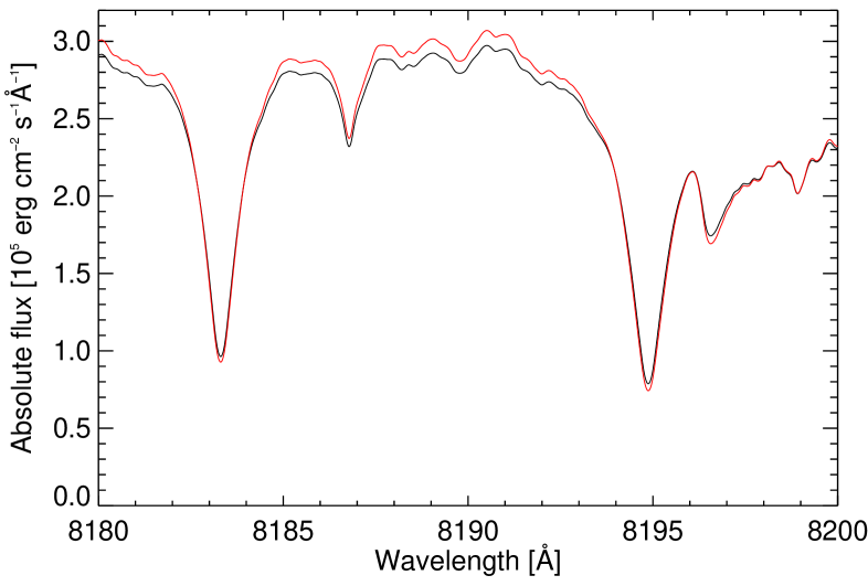
Figure 19: Comparison of synthetic spectra showing a subordinate Na i doublet (at 8183.3, 8194.8 Å) based on hydrodynamical model C3 (black solid line) and a corresponding mixing-length model with $\alpha_{\mathrm{MLT}}=1.5$ (grey solid line, red in color version).

We find that, accounting for the hydrodynamical structure, yields systematically weaker TiO (and H₂O not shown) bands by 0.18 and 0.025 dex respectively, while the pseudo-continuum appears unchanged. This is possible because the strongest TiO bands are formed at two dex lower optical depth than the opacity minima between those bands. The differences in the strength of the epsilon subband heads in the synthetic spectra of Fig. 18 would correspond to a difference in $T_{\mathrm{eff}}$ of $\approx 200\mbox{\rm\,K}$ when compared to an observed spectrum, in the sense that an analysis based on MLT models overestimates $T_{\mathrm{eff}}$.

Atomic lines absorbing through TiO bands troughs such has the doublets of Ti at $\lambda\lambda$ 8435.7, 8435.0 Å, of K i at $\lambda\lambda$ 7664.9, 7699.0 Å, and all other atomic lines formed bluewards of 0.7 $\mu$m, would look wider and deeper in contrast to the TiO pseudo-continuum, causing MLT models to overestimate gravities. This is not the case of the Na i doublet at $\lambda\lambda$ 8183.3, 8194.8 Å shown in Fig. 19 which is practically unaffected by this pseudo-continuum because it forms between TiO and VO band heads from deeper photospheric layers. The same would be true of lines formed around the peak of the spectral distribution between 0.9 and 1.3 $\mu$m. Although of course these can be as well affected in analysis where $T_{\mathrm{eff}}$ is determined from the TiO bands.

5 Mixing by atmospheric overshoot

For describing the mixing properties of the flow field in the overshooting layers of our models, we follow the approximate procedure laid out by LAH. We describe the mixing in terms of a mass exchange frequency given by

$$f_{\mathrm{ex}}(z)\equiv\frac{\langle F_{\mathrm{mass}}^{\mathrm{up}}\rangle(z)}{\langle m_{\mathrm{col}}\rangle(z)}.$$ (2)

$F_{\mathrm{mass}}^{\mathrm{up}}$ is the upward directed component of the mass flux

$$F_{\mathrm{mass}}^{\mathrm{up}}(x,y,z,t)\equiv\left\{\begin{array}[]{ll}\rho v_{\mathrm{z}}&\mathrm{if}\hskip 4.30554ptv_{\mathrm{z}}>0\\ 0&\mathrm{otherwise}.\end{array}\right.$$ (3)

where $v_{\mathrm{z}}$ is the vertical component of the velocity (counted as positive if directed upwards), $\rho$ the mass density, $x$, $y$, $z$ the spatial coordinates, and $t$ the time. $m_{\mathrm{col}}$ is the mass column density given by

$$m_{\mathrm{col}}(x,y,z,t)\equiv\int_{z}^{\infty}\!dz^{\prime}\,\rho(x,y,z^{\prime},t).$$ (4)

$\langle.\rangle$ denotes the horizontal and temporal average over $x$, $y$, and $t$. The basic idea is to take the time scale over which the mass above a certain reference height is potentially exchanged by the flow as time scale over which material is mixed with fresh material stemming from the deeper lying, convective layers. As we shall see the mass exchange frequency $f_{\mathrm{ex}}$ exhibits an exponential height dependence. The mixing rate given by relation (2) is an approximation only. Depending on the way the mixing takes place in detail, the normalization of the mixing profile might change. However, the relative shape of the mixing rate – the exponential decline – is a robust feature, and in the following we shall characterize the mixing found in our models by the scale height of the exponential decline.

We note that in Ludwig (2003) the mixing was described in terms of a mixing velocity

$$v_{\mathrm{mix}}\equiv\frac{\langle F_{\mathrm{mass}}^{\mathrm{up}}\rangle}{\langle\rho\rangle}$$ (5)

where $\rho$ denotes the mass density. $v_{\mathrm{mix}}$ also shows an exponential height dependence, and its rate of decline was given in the above paper. While at the level of our approximation the description in terms of $v_{\mathrm{mix}}$ is equivalent to the one in terms of $f_{\mathrm{ex}}$, the scale heights of the various declines can differ substantially. Differences become large in cases where the scale heights of $v_{\mathrm{mix}}$ or $f_{\mathrm{ex}}$ are large, or the scale heights of $\rho$ and $m_{\mathrm{col}}$ differ noticeably.

5.1 Subsonic filtering

The atmospheric velocity field is a superposition of advective motions and acoustic waves generated by convection in deeper layers (see also LAH, and Ludwig & Nordlund 2000). The wave motions contribute little if at all to the mixing due to their spatially coherent, oscillatory character. The overshooting, convective motions tend to decay with distance to the Schwarzschild stability boundary, while the wave amplitudes tend to increase with height due to the sharp decrease in mass density. This leads to the situation that beyond a certain height the atmospheric velocity field becomes dominated by wave motions. In order to get a reliable estimate of the mixing, it is therefore necessary to remove the wave contributions to the velocity field before evaluating the mass flux $F_{\mathrm{mass}}^{\mathrm{up}}$.

We removed the wave contributions by subsonic filtering – a technique developed in the context of solar observations for cleaning images from “noise” stemming from the solar 5 minute oscillations (Title et al. 1989). Figure 20 schematically illustrates this filtering technique. In short, one considers a time sequence of images and removes features with horizontal phase speeds $v_{\mathrm{phase}}$ greater than a prescribed threshold. This is achieved by Fourier filtering of spatial-temporal data in the $k$-$\omega$ domain. For every depth layer in our data cubes we performed a 3D Fourier analysis (one temporal, two spatial dimensions) of the vertical mass flux retaining only contributions below a preset phase speed threshold. In practice, acoustic and convective contributions are not as cleanly separated as shown in the Fig. 20, and one must find the right balance between removing as much acoustic components as possible while retaining as much as possible convective contributions. We always studied a sequence of phase speed thresholds in order to judge the success of the procedure.

Figure 20: Schematic illustration of subsonic filtering in the $k$-$\omega$ domain: only components in wavenumber-frequency domain below a prescribed phase speed $v_{\mathrm{phase}}$ are retained. They preferentially belong to convective motions.

5.2 Mixing in the solar atmosphere

For reference we begin with a discussion of the mixing in the solar atmosphere. Figure 21 shows $f_{\mathrm{ex}}$ in our solar model for various degrees of subsonic filtering. It is clearly visible that the subsonic filtering has the strongest impact on $f_{\mathrm{ex}}$ in the uppermost atmospheric layers. As hinted above, $f_{\mathrm{ex}}$ exhibits an exponential decline with height ($\log P\propto z$) after appropriate subsonic filtering which was put forward by Freytag et al. (1996) as generic feature of convective overshoot. Figure 21 further shows that too low a velocity threshold removes also convective features, as visible by the reduction of the velocity in the deeper, convection dominated layers for the case of a phase speed threshold of 1.5 km s^-1. Quantitatively, for the Sun we find a scale height of $f_{\mathrm{ex}}$ in terms of the local pressure scale height of $H_{\mathrm{fex}}=2.4\,H_{\mathrm{P}}$ with an uncertainty of about 10 %.

Apart from purely numerical findings, an exponential decline of $f_{\mathrm{ex}}$ is also motivated from semi-analytical considerations of the behavior of linear convective modes (Freytag et al. 1996). In Fig. 21 we plotted the $f_{\mathrm{ex}}$-profile of a linear convective eigenmode with horizontal wavelength of $\lambda_{\mathrm{mode}}=5.0\mbox{\rm\,Mm}$. We used the temporally and horizontally averaged hydrodynamical structure as background on which we solved the linearized hydrodynamical equations. The absolute amplitude of the mode has been scaled to match $f_{\mathrm{ex}}$ of the hydrodynamical model leaving the shape of the mode’s $f_{\mathrm{ex}}$-profile intact. The exchange frequency of the mode exhibits an exponential “leakage” into the formally convective stable layers. Generally, the rate of decline depends on $\lambda_{\mathrm{mode}}$, being faster for modes of shorter horizontal wavelengths. The mode with 5.0 Mm wavelength was chosen since it provided a good overall fit to the decline of $f_{\mathrm{ex}}$ in the hydrodynamical model. The wavelength of this mode is significantly larger than the horizontal scale of the dominant convective structures on the Sun – the granules with typical sizes of around 1.2 Mm. This might be related to the assumption of adiabaticity in the mode calculations, which is not a good approximation in the solar photosphere, or to the fact that a convective mode is a non-stationary solution of the hydrodynamical equations.

From the rather large wavelength of the best fitting mode one might argue that 5.0 Mm is close to the geometrical size of the computational box of model S (6.0 Mm), and actually the box size sets the rate of decline of $f_{\mathrm{ex}}$. We verified that a solar model of about twice the horizontal size gives the same rate of decline as model S. The box size of model S is sufficient to allow the build-up of all convective structures contributing significantly to the overshooting velocity field in the deep photosphere. The box sizes of the M-type models are allowing the presence of a similar number of convective cells as the solar model. Thus, we expect that also our M-type models capture the relevant convective structures controlling the overshooting motions.

Figure 21: Mass exchange frequency $f_{\mathrm{ex}}$ in solar model S as a function of gas pressure: the unfiltered data (thick solid line) were subsonically filtered retaining only features with phase speeds $v_{\mathrm{phase}}<$ 12, 6, 3, and 1.5 km s^-1 (thin solid lines from top to bottom). The approximate location of the Schwarzschild boundary of convective stability is indicated by the dotted vertical line, $f_{\mathrm{ex}}$ of a convective eigenmodes with horizontal wavelength $\lambda_{\mathrm{mode}}=5.0\mbox{\rm\,Mm}=33\,H_{\mathrm{P}}^{\mathrm{surf}}$ by the dashed line. The dash-dotted line is a fit depicting the decline of $f_{\mathrm{ex}}$. It is labeled by the scale height of the decline in units of the local pressure scale height. The pressure is given in units of the pressure at Rosseland optical depth unity $P_{\mathrm{surf}}$. The plateau at lowest pressures is an artifact of the upper boundary condition applied in the RHD model.

5.3 Mixing in M-type atmospheres

In Fig. 22 and 23, we show the vertical distribution of the mass-exchange rates $f_{\mathrm{ex}}$ for two of our M-type models. With decreasing $\log g$ and increasing $T_{\mathrm{eff}}$, the zone of convective instability extends further and further into the optically thin atmosphere, leaving little room for overshoot in the models C3 and H4. Reading off an exponential decline rate is very uncertain in these models. However, from them we find a slow decline with $H_{\mathrm{fex}}\approx 18\,H_{\mathrm{P}}$ in C3 and $\approx 28\,H_{\mathrm{P}}$ in H4. Models C3 and C4 leave more room for overshooting, allowing a more precise determination of the exponential decline. We estimate the involved uncertainty to about 20 %. We find $H_{\mathrm{fex}}=0.5\,H_{\mathrm{P}}$ in model  C5 and $3.2\,H_{\mathrm{P}}$ in C4. Note, that in the model C5 with highest gravity and steepest decline of $f_{\mathrm{ex}}$ the exponential behavior does not set in immediately at the boundary of convective stability

Qualitatively, in terms of the rate of decline, overshooting is less pronounced in models of higher gravity. This is in part due to the fact that buoyancy forces scale proportional to gravity, making buoyancy more effective in confining the convective motions to the formally unstable regions. At lower gravity, mixing – despite the increasing geometrical scales – is more rapid, not only due to the slower decline of the mixing rate but also due to the higher convective velocities.

Silicate cloud formation is one of the most important aspect of the modeling of late-type M and brown dwarfs. The formation of clouds is understood as a compromise between condensation, sedimentation and advection (turbulent overshooting mixing) time scales which determine the extension, location in the thermal atmospheric structure, and composition of the cloud deck. To represent the correct distribution with height of the mixing time scale, investigators have experimented with various descriptions for $f_{\mathrm{ex}}$: Allard et al. (2003) used a parabolic function with opening set by the innermost and outermost convective layers, and normalized at the convective velocity maximum, while Ackerman & Marley (2001) and Cooper et al. (2003) preferred a constant distribution throughout the atmosphere, set to the value associated with the maximum of the convective velocity. A modeling with convective modes should give a more physical description which could be implemented in 1D model atmospheres. Trying to match the mixing profiles in the overshooting regions with convective modes, however, worked only partially so far. For the lower gravity models the fits were not satisfactory. This might be related to the situation that convection reaches high up, and we do not actually see the asymptotic exponential tail of the mixing profile. We oriented the horizontal wavelength of the linear modes at the largest sizes of structures the computational box could accommodate in the respective models. Despite the present shortcoming we are optimistic that one can add refinements to the mode-modelization that would allow to satisfactorily match the RHD results.

If the mixing trends observed in our models hold for cooler objects, these go in the direction of making clouds thicker or more extended into higher atmospheric layers with decreasing gravities and increasing $T_{\mathrm{eff}}$ . However, decreasing pressure will work in the opposite direction, making it harder for grains to form. Detailed calculations will be presented in a subsequent publication. Nevertheless, we expect that clouds will be more extended for young objects than for older ones of same $T_{\mathrm{eff}}$, and that these will remain dusty at lower $T_{\mathrm{eff}}$ and later spectral types, i.e, below spectral class T4 or 1400 K (Golimowski et al. 2004).

Figure 22: Like Fig. 21, model C5. $v_{\mathrm{phase}}<$ 1.0, 0.5, 0.25 km s^-1, $\lambda_{\mathrm{mode}}=250\mbox{\rm\,km}=22\,H_{\mathrm{P}}^{\mathrm{surf}}$.

Figure 23: Like Fig. 21, model C4. $v_{\mathrm{phase}}<$ 8.0, 4.0, 2.0, 1.0, 0.5 km s^-1, $\lambda_{\mathrm{mode}}=3.0\mbox{\rm\,Mm}=24\,H_{\mathrm{P}}^{\mathrm{surf}}$.

5.4 Cloud cover disruption in early T-type brown dwarfs

Burgasser et al. (2002) have found a resurgence of molecular spectral features such as FeH bands in the spectra of early T-type brown dwarfs. This is interpreted as a spectral signature of the onset of cloud cover disruption. Indeed, these spectral features of refractory species can only be seen if the atmosphere is transparent enough to observe flux emerging from below the cloud forming layers. This is possible if holes in the cloud deck are occurring.

Dust does not form in the models studied in this work. However, here we want to speculate how the cloud pattern might look when one expects a disrupted cloud layer like in early T-dwarfs. The cloud deck is shaped by convective overshooting which mixes up refractory material into the grain condensing part of the atmosphere – below gas temperatures of 2000 K, in early T-dwarfs perhaps over one pressure scale height above the convectively unstable layers. This far above the convection zone, the horizontal and vertical motions are not correlated in the same way as in the strongly convective layer where the flow forms cell-like patterns. Structures larger than the granular scale in combination with waves dominate the velocity field. The typical granular flow pattern is ”washed out” from the flow higher up. Hence, we do not expect that the cloud deck is fragmented on a spatial scale given by the granular scale, but likely on a larger scale. This consideration refers to effects of convection. It is of course well possible that the actual cloud pattern is rather shaped by the global wind circulation expected to be present in rotating brown dwarfs or planets.

6 Final remarks

We have seen that mixing-length theory provides a reasonably realistic picture of the convective energy transport in M-type atmospheres, even considering that a substantial part of the optically thin atmosphere is affected by convection. However quantitatively, temperature errors of up to $\approx 250\mbox{\rm\,K}$ (or 9 %) are possible if one (unluckily) picked a value of unity for the mixing-length parameter ($\alpha_{\mathrm{MLT}}$) entering MLT. The efficiency of the convective energy transport measured in terms of an effective mixing-length parameter is rather high in M-type atmospheres. Choosing a larger $\alpha_{\mathrm{MLT}}$ helps but is not sufficient to describe the thermal structure of M-type atmospheres if one wishes to attain a high level of accuracy. MLT does not provide the precise scaling of the convective transport efficiency with stellar parameters and optical depth. To get a better quantitative description one might try to calibrate besides $\alpha_{\mathrm{MLT}}$ the “internal” parameters of MLT with radiation-hydrodynamics models. M-type atmospheres appear particularly well suited for this undertaking since convection takes place under optically thick and thin conditions.

Our results have shown that convective overshooting mixes the layers of M-type atmospheres which are formally (according to the Schwarzschild criterion) stable against convection much more strongly towards higher effective temperatures and lower gravities. This should make young late-type M-dwarfs and brown dwarfs even more cloudy than older disk objects of the same $T_{\mathrm{eff}}$. We think that a detailed modeling of such cooler atmospheres, especially around 1400 K should deliver important clues about the interesting question of the cloud cover, and should help to understand the break in colors and spectral type vs. effective temperature relation observed for these objects (Knapp et al. 2004; Golimowski et al. 2004).

To aid the modeling of the spectral properties of cloudy objects, we further think it should be worthwhile to improve the model of convective modes which where mostly used for demonstration purposes in this work. Our current mode model did not perform sufficiently to be up to the task but a number of refinements can be brought to this model and tested. It could be calibrated with RHD models in a similar fashion like MLT. At a higher ambition level one might even contemplate to combine ideas into a single description for the energy transport and effects related to overshooting. We are aware that many attempts have been made to improve or even completely replace MLT since it has been introduced into astrophysics in the early 1950s by Böhm-Vitense – with mixed success. Our goal would not be to formulate a new convection theory but rather a parameterized model like MLT which is flexible enough to fully fit RHD results, and contains sufficient physics to allow a robust inter- and extrapolation in a wide range of stellar parameters. The availability of detailed RHD models appear essential to identify the necessary building blocks.

The main uncertainty affecting our present results is related to the approximate treatment of the wavelength-dependence of opacity in the radiative transfer which was optimized for an atmosphere at $T_{\mathrm{eff}}$=2900 K and $\log g$=5.3. So, one of the first issues to be addressed in future work is the improvement of this approach. Work is under way for a refined implementation in a new 3D radiation-hydrodynamics code (named CO⁵BOLD, Freytag et al. 2002; Wedemeyer et al. 2004). We finally emphasize that our results apply to atmospheres of solar metalicity. We expect marked differences for metal-poor atmospheres (see, e.g., Asplund et al. 1999).

Appendix A Computation of the Péclet number

The Péclet number $\mathrm{Pe}$ measures the relative importance between conductive (here by radiation) and advective heat transport

$$\mathrm{Pe}\equiv\frac{t_{\mathrm{rad}}}{t_{\mathrm{adv}}}.$$ (6)

$t_{\mathrm{rad}}$ is a radiative relaxation time, and $t_{\mathrm{adv}}$ a characteristic time over which the temperature of moving gas elements changes due to adiabatic compression or expansion. In the present context, we employ a mixing-length picture and evaluate the radiative relaxation time $t_{\mathrm{rad}}$ with the MLT formula

$$t_{\mathrm{rad}}=\frac{\rho c_{\mathrm{p}}\Lambda\tau_{\mathrm{e}}}{f_{3}\sigma\chi T^{3}}\,\left(1+\frac{f_{4}}{\tau_{\mathrm{e}}^{2}}\right).$$ (7)

$c_{\mathrm{p}}$ denotes the specific heat at constant pressure, $\Lambda=\alpha_{\mathrm{MLT}}H_{\mathrm{P}}$ the mixing-length, $\sigma$ Stefan-Boltzmann’s constant, $\chi$ opacity, $T$ temperature, $\rho$ mass density, and $\tau_{\mathrm{e}}$ the optical thickness of a convective element defined as

$$\tau_{\mathrm{e}}\equiv\chi\rho\Lambda.$$ (8)

$f_{3}=16$ and $f_{4}=2$ are dimensionless constants set to values assumed in the MLT formulation of Mihalas (see Ludwig et al. 1999). We further assume a mixing-length parameter $\alpha_{\mathrm{MLT}}=2.5$ which is a reasonable value for the M-type atmospheres under consideration (see Fig. 13).

Similarly, we estimate $t_{\mathrm{adv}}$ as the time interval over which a vertically moving gas element has build up a substantial temperature difference according to

$$t_{\mathrm{adv}}=\frac{\Lambda}{v_{\mathrm{c}}}$$ (9)

where $\nabla$ is the logarithmic temperature derivative of the thermal profile with respect to pressure, $\nabla_{\mathrm{ad}}$ the corresponding adiabatic value, and $v_{\mathrm{c}}$ a convective velocity we set to a typical atmospheric value (300 m s^-1 for model C5 and 600 m s^-1 for model C3, see Fig. 17). Note, that in this paper we argue taking recourse to ratios of $\mathrm{Pe}$ only. This makes the precise choice of arbitrary or little constrained parameters less critical.

References

- Ackerman & Marley (2001) Ackerman, A. S. & Marley, M. S. 2001, ApJ, 556, 872
- Allard et al. (2003) Allard, F., Guillot, T., Ludwig, H.-G., et al. 2003, in IAU Symposium No. 211: Brown Dwarfs, 325
- Asplund et al. (1999) Asplund, M., Nordlund, Å., Trampedach, R., & Stein, R. F. 1999, A&A, 346, L17
- Baraffe et al. (2002) Baraffe, I., Chabrier, G., Allard, F., & Hauschildt, P. 2002, A&A, 382, 563
- Böhm-Vitense (1958) Böhm-Vitense, E. 1958, Zs. f. Ap., 46, 108
- Burgasser et al. (2002) Burgasser, A. J., Marley, M. S., Ackerman, A. S., et al. 2002, ApJL, 571, L151
- Cattaneo et al. (1991) Cattaneo, F., Brumell, N., Toomre, J., Malagoli, A., & Hurlburt, N. 1991, Astrophys. J., 370
- Chan & Sofia (1987) Chan, K. & Sofia, S. 1987, Science, 235, 465
- Chan & Sofia (1989) Chan, K. & Sofia, S. 1989, Astrophys. J., 336, 1022
- Cooper et al. (2003) Cooper, C. S., Sudarsky, D., Milsom, J. A., Lunine, J. I., & Burrows, A. 2003, ApJ, 586, 1320
- Ferguson et al. (2005) Ferguson, J. W., Alexander, D. R., Allard, F., et al. 2005, Astrophys. J., 623, 585
- Freytag et al. (1996) Freytag, B., Ludwig, H.-G., & Steffen, M. 1996, A&A, 313, 397
- Freytag et al. (2002) Freytag, B., Steffen, M., & Dorch, B. 2002, AN, 323, 213
- Gadun & Pikalov (1996) Gadun, A. & Pikalov, K. 1996, Solar Phys., 166, 569
- Golimowski et al. (2004) Golimowski, D., Leggett, S., Marley, M., et al. 2004, AJ, 127, 3516
- Hauschildt et al. (1999) Hauschildt, P., Allard, F., & Baron, E. 1999, Astrophys. J., 512, 377
- Helling et al. (2004) Helling, C., Klein, R., Woitke, P., Nowak, U., & Sedlmayr, E. 2004, AA, 423, 657
- Kim et al. (1995) Kim, Y.-C., Fox, P., Sofia, S., & Demarque, P. 1995, Astrophys. J., 442, 422
- Knapp et al. (2004) Knapp, G., Leggett, S., Fan, X., et al. 2004, AJ, 127, 3553
- Ludwig (1992) Ludwig, H.-G. 1992, Ph.D. Thesis (University of Kiel)
- Ludwig (2003) Ludwig, H.-G. 2003, in Proceedings of the IAU Symposium: Modelling of Stellar Atmosperes, ed. N. Piskunov, W. Weiss, & D. Gray (Astronomical Society of the Pacific), 113
- Ludwig et al. (2002) Ludwig, H.-G., Allard, F., & Hauschildt, P. 2002, A&A, 395, 99
- Ludwig et al. (1999) Ludwig, H.-G., Freytag, B., & Steffen, M. 1999, A&A, 346, 111
- Ludwig et al. (1994) Ludwig, H.-G., Jordan, S., & Steffen, M. 1994, A&A, 284, 105
- Ludwig & Nordlund (2000) Ludwig, H.-G. & Nordlund, Å. 2000, in Pacific Rim Conference on Stellar Astrophysics, ed. K. Cheng, H. Chau, & K. Chan (Kluver Academic Publishers), 37–44
- Mihalas (1978) Mihalas, D. 1978, Stellar Atmospheres (Freeman and Company)
- Mohanty et al. (2004) Mohanty, S., Basri, G., Jayawardhana, R., et al. 2004, Astrophys. J., 609, 854
- Nordlund (1982) Nordlund, Å. 1982, A&A, 107, 1
- Nordlund & Dravins (1990) Nordlund, Å. & Dravins, D. 1990, AA, 228, 155
- Press et al. (1992) Press, W., Teukolsky, S., Vetterling, W., & Flannery, B. 1992, Numerical Recipes in Fortran (Cambridge University Press)
- Robinson et al. (2003) Robinson, F., Demarque, P., Li, L., et al. 2003, MNRAS, 340, 923
- Robinson et al. (2004) Robinson, F., Demarque, P., Li, L., et al. 2004, MNRAS, 347, 1208
- Singh & Chan (1993) Singh, H. & Chan, K. 1993, A&A, 279, 107
- Steffen (1993) Steffen, M. 1993, in Inside the stars, ed. W. Weiss & A. Baglin (ASP Conference Series, vol. 40), 300
- Steffen et al. (1995) Steffen, M., Ludwig, H.-G., & Freytag, B. 1995, A&A, 300, 473
- Steffen et al. (1989) Steffen, M., Ludwig, H.-G., & Krüß, A. 1989, A&A, 213, 371
- Stein & Nordlund (1998) Stein, R. F. & Nordlund, Å. 1998, Astrophys. J., 499, 914
- Steiner et al. (1998) Steiner, O., Grossmann-Doerth, U., Knoelker, M., & Schüssler, M. 1998, ApJ, 495, 468
- Title et al. (1989) Title, A. M., Tarbell, T. D., Topka, K. P., Ferguson, S. H., & Shine, R. A. 1989, Astrophys. J., 336, 475
- Tsuji (2005) Tsuji, T. 2005, ApJ, 621, 1033
- Vögler et al. (2004) Vögler, A., Bruls, J., & Schüssler, M. 2004, AA, 421, 741
- Vögler & Schüssler (2003) Vögler, A. & Schüssler, M. 2003, AN, 324, 399
- Wedemeyer et al. (2004) Wedemeyer, S., Freytag, B., Steffen, M., Ludwig, H.-G., & Holweger, H. 2004, A&A, 414, 1121