Monte Carlo Simulations of Globular Cluster Evolution. IV.
Direct Integration of Strong Interactions

Abstract

We study the dynamical evolution of globular clusters containing populations of primordial binaries, using our newly updated Monte Carlo cluster evolution code with the inclusion of direct integration of binary scattering interactions. We describe the modifications we have made to the code, as well as improvements we have made to the core Monte Carlo method. We present several test calculations to verify the validity of the new code, and perform many comparisons with previous analytical and numerical work in the literature. We simulate the evolution of a large grid of models, with a wide range of initial cluster profiles, and with binary fractions ranging from 0 to 1, and compare with observations of Galactic globular clusters. We find that our code yields very good agreement with direct $N$-body simulations of clusters with primordial binaries, but yields some results that differ significantly from other approximate methods. Notably, the direct integration of binary interactions reduces their energy generation rate relative to the simple recipes used in Paper III, and yields smaller core radii. Our results for the structural parameters of clusters during the binary-burning phase are now in the tail of the range of parameters for observed clusters, implying that either clusters are born significantly more or less centrally concentrated than has been previously considered, or that there are additional physical processes beyond two-body relaxation and binary interactions that affect the structural characteristics of clusters.

1. Introduction

Observations (e.g., Cote et al., 1996; Bellazzini et al., 2002b; Rubenstein & Bailyn, 1997; Cool & Bolton, 2002; Bellazzini et al., 2002a), in combination with recent theoretical work (Ivanova et al., 2005), suggest that although the currently observed binary fractions in the cores of globular clusters may be small ($\lesssim 10\%$), the initial cluster binary fraction may have been significantly larger ($\gtrsim 50\%$). As has been understood theoretically for some time, primordial binaries in star clusters generally act as an energy source (through super-elastic scattering encounters), producing energy in the core and postponing deep core collapse in a quasi-steady state “binary-burning” phase. This is analogous to the long-lived main-sequence in stars, in which hydrogen is burned to prevent collapse. An initial binary fraction of a few percent is enough to postpone deep core collapse for many initial relaxation times (see Fregeau et al., 2003, for discussion and references). In addition to playing a large part in the global evolution of a star cluster, dynamical interactions of binaries also strongly affect the formation and evolution of stellar and binary exotica, which include low-mass X-ray binaries, recycled pulsars, cataclysmic variables, and blue stragglers (Hut et al., 1991; Sigurdsson & Phinney, 1995; Davies & Hansen, 1998; Rasio et al., 2000; Ivanova et al., 2005).

Similarly to dynamical binary interactions, physical stellar collisions (both direct star–star collisions, and those mediated by resonant binary interactions) also play an important role in the evolution of globular cluster populations. Stellar collisions are thought to be one of the two primary mechanisms by which blue stragglers are created in dense star clusters (e.g., Mapelli et al., 2004). A runaway sequence of stellar collisions of massive main sequence stars early in the lifetime of a dense cluster may yield a very massive star ($\gtrsim 10^{3}\,M_{\sun}$), which may then become an intermediate mass black hole (see, e.g., Gürkan et al., 2006, for discussion and references).

The complete picture of star cluster evolution can be rather complicated, as it includes, in addition to the two physical processes just mentioned, single star evolution, binary star evolution, and tidal stripping due to the field of the Galaxy. Even if one ignores these additional processes, modeling a dense stellar cluster with primordial binaries still presents a formidable computational challenge. There are at least two reasons for this: 1) dynamical interactions of binaries—which are typically resonant, lasting for many orbits—must be resolved on their natural timescale, which is orders of magnitude shorter than the cluster relaxation time, and 2) primordial binaries extend the life of a cluster. Although the GRAPE series of special-purpose computers is steadily increasing in performance, direct $N$-body simulation of the evolution of clusters with more than a few percent binaries and a moderate number of stars ($\sim 10^{5}$) is still quite computationally expensive, with computational timescales on the order of months. Faster, more approximate methods, such as the anisotropic gas model or direct solution of the Fokker-Planck equation, suffer from the difficulty inherent in incorporating physics beyond two-body relaxation, such as stellar evolution or binary interactions, in these methods. The Monte Carlo method bridges the gap between these two computational extremes, since it allows for the relatively facile inclusion of additional layers of physics, provides a star-by-star description of a cluster, and is computationally inexpensive.

In previous studies using approximate methods like Monte Carlo or Fokker-Planck, binary interactions had generally been treated using recipes culled from the results of large numbers of numerical scattering experiments. (The work of Giersz & Spurzem (2003), which incorporates direct integration of binary interactions, is one notable exception.) The recipes are typically known only for equal-mass binary interactions, thus prohibiting the use of a cluster mass function. Thus in order to model realistic clusters, which contain a wide range of masses, one must numerically integrate each binary interaction in order to resolve it properly. We have now incorporated into our Monte Carlo code a dynamical integrator to exactly integrate dynamical interactions of binaries, allowing us to evolve clusters with mass spectra, and perform more realistic comparisons with direct $N$-body calculations. As we demonstrate below, the direct integration of binary interactions reduces their energy generation rate relative to the simple recipes used in Paper III, and yields smaller core radii.

This is the fourth paper in a series studying the evolution of globular clusters using the Monte Carlo method. Paper I describes the core method and presents several test calculations exhibiting the validity of the code (Joshi et al., 2000). Paper II treats the evolution of tidally-truncated clusters with mass spectra (Joshi et al., 2001). Paper III adds a recipes-based treatment of binary scattering interactions and considers the evolution of an ensemble of clusters of varying initial binary fraction and central concentration, finding that even a small fraction of binaries in a cluster is sufficient to support the core against collapse significantly beyond the normal core-collapse time (Fregeau et al., 2003, hereafter Paper III). In this, the fourth paper in the series, we describe our new code, perform several tests to ensure its validity, and perform a large set of simulations of clusters with primordial binaries, which we compare with previous results in the literature and with observations of Galactic globular clusters. Section 2 describes our new code in detail, including the additional physical processes we have added (numerical integration of binary scattering interactions, and star–star physical collisions), as well as the improvements we have made to the core Monte Carlo method. Section 3 presents a few example results, and compares them with semi-analytical theory and previous numerical calculations. Section 4 describes the trends evident in the grid of cluster models we simulated, and compares our results with observations. Finally, in section 5 we summarize and conclude.

2. Method

Here we describe in detail our implementation of the Monte Carlo numerical method for simulating the evolution of dense star clusters. It incorporates many physical processes of relevance in dense star clusters, including two-body relaxation, direct physical stellar collisions, and dynamical interactions of binaries. Each of these physical processes is treated sufficiently accurately so as to allow for a rather wide mass spectrum (e.g., $M_{\rm max}/M_{\rm min}\sim 10^{3}$ for a Salpeter mass function). For now we neglect stellar evolution (both single and binary), but plan to include it in our code in the near future. Those readers uninterested in the technical details of our numerical method can safely skip ahead to the next section.

2.1. Units

Before describing our method in detail, we discuss a necessary formality. We use the standard $N$-body system of units (Heggie & Mathieu, 1986; Heggie & Hut, 2003). For reasons of convenience, we use two units of time in our code. In addition to the standard $N$-body unit of time (which is roughly the crossing time), we use the relaxation time. Thus our full (over-specified) system of units is given by the standard formulae:

$$U_{m} = M_{0}$$ (1)

$$U_{l} = \frac{GM_{0}^{2}}{-4E_{0}}$$ (2)

$$U_{t} = \frac{GM_{0}^{5/2}}{(-4E_{0})^{3/2}}$$ (3)

$$U_{t_{\rm rel}} = \frac{N_{0}}{\ln\gamma N_{0}}U_{t}\,,$$ (4)

where $M_{0}$ is the initial total mass of the cluster, $E_{0}$ is the initial total energy of the cluster, $N_{0}$ is the initial number of stars, and $\gamma N_{0}$ is the Coulomb logarithm. The quantity $\gamma$ is a function of the initial structure of the cluster, and is only needed when converting time in code units to physical units. Thus it does not need to be specified for purely relaxation calculations, which can be quoted in units of the relaxation time, but it does need to be specified for calculations which include additional physics, like physical collisions and binary interactions. For our simulations we set $\gamma$ via comparisons with $N$-body results (where available), as discussed later.

2.2. Standard Definitions

It is often useful to be explicit about how certain derived measurable quantities are calculated. For the half-mass relaxation time we adopt the standard definition (Spitzer & Hart, 1971):

$$t_{\rm rh}=\frac{0.138N}{\ln(\gamma N)}\left(\frac{r_{h}^{3}}{GM}\right)^{1/2}\,,$$ (5)

where $N$ is the number of bound cluster objects (single star or binary), $r_{h}$ is the radius containing half the mass of the cluster, and $M$ is the total cluster mass. Most plots presented in this paper use as time unit the initial half-mass relaxation time, i.e. $t_{\rm rh}$ evaluated at the start of the simulation. For the core radius we use the density-weighted average described in Casertano & Hut (1985), with $j=6$ and where the averaging is performed from the cluster center out to the half mass radius. In this scheme, a local density is estimated for each star in the cluster by taking the average density within a sphere centered on the star with radius at the $j$th star. The core radius is then estimated by taking the local density weighted average of star position out to the half mass radius. We use the same density-weighted averaging scheme to estimate the central density, velocity dispersion, and average mass, except in places where otherwise noted. In some cases, as described in the text, we also plot the core radius as measured by the standard definition (Spitzer, 1987):

$$r_{c}=\left(\frac{3\sigma_{0}^{2}}{4\pi G\rho_{0}}\right)^{1/2}\,,$$ (6)

where $\sigma_{0}$ is the central three-dimensional velocity dispersion, and $\rho_{0}$ is the central mass density. Note that the results we compare with below from Heggie et al. (2006) adopt the density-weighted average definition of the core radius. As shown in Fig. 13, the two definitions differ minimally when the cluster is in the binary burning phase.

2.3. Two-Body Relaxation

Two-body relaxation is the primary physical process responsible for the diffusion of energy in a star cluster, and thus for its global evolution (Heggie & Hut, 2003). We use the Hénon orbit-averaged Monte Carlo method to simulate two-body relaxation (Hénon, 1971). For a detailed description of the basic method we employ, see Joshi et al. (2000). In summary, a timestep in the code consists of the following:

1. Using each star’s radial position $r$ and mass $m$, the potential $\Phi(r)$ is calculated under the assumption of spherical symmetry (each star is represented by an infinitesimally thin spherical shell).

2. Each pair of stars neighboring in radius undergoes a hyperbolic “super”-encounter, with scattering angle chosen so as to represent the cumulative effect on each star of many long-range, small-angle two-body scattering encounters with all other stars in the system.

3. Using the new radial velocity $v_{r}$ and tangential velocity $v_{t}$, the new specific energy $E$ and angular momentum $J$ of each star is calculated (using $\Phi(r)$ from step 1).

4. A new position and corresponding velocity is chosen for each star by picking a point on its orbit randomly, sampled in accordance with the amount of time spent at each radial position (i.e., weighted by $1/v_{r}$).

We have made two improvements to the fundamental method which were necessary to accurately treat star clusters with wide mass spectra, and for the stability of the long-term evolutions needed for clusters with primordial binaries.

The first improvement is a rather simple one that provides for self-consistency in step 4 above. Solving for the new position of a star along its orbit appears to be a straightforward matter: using the potential calculated in step 1, one writes down the energy equation for the orbit, $E=\Phi(r)+J^{2}/2r^{2}+\frac{1}{2}v_{r}^{2}$, solves for the pericenter and apocenter, then samples the radial position with a weighting inversely proportional to $v_{r}$. However, the potential calculated in step 1 includes the contribution from the star whose orbit we are trying to solve. In other words, the star on its orbit feels the gravitational effect of itself at its old position. This inconsistency is ignored in the standard Monte Carlo method (Hénon, 1971; Joshi et al., 2000), although it is corrected in the new Monte Carlo code of Freitag & Benz (2001). Neglecting this inconsistency for the case of equal-mass clusters produces a minimal effect on the overall evolution, slightly postponing core collapse, and leading to a steady drift in the total system energy. However, when one considers clusters with even modestly wide mass spectra ($\sim 0.1$–$10\,M_{\sun}$), the errors are much less benign. Since the most massive stars in the mass spectrum contribute proportionately more to the cluster potential, it is the calculation of their orbits that is most inaccurate. In our simulations we have seen that as the mass spectrum is widened, the core collapse time gets progressively longer than what would be expected—from direct $N$-body results and the Monte Carlo calculations of Freitag et al. (2006b)—until it is prevented completely. In other words, this inconsistency acts as a spurious energy source, postponing core collapse.

Correcting the inconsistency in the potential is straightforward. We simply add a correction term to the potential when solving for a star’s orbit. For star $j$ with mass $m_{j}$, originally at position $r_{j}$ when the potential was last calculated, the correction term is

$$\Phi_{s}(r)=\begin{cases}\displaystyle\frac{Gm_{j}}{r}&r\geq r_{j}\\ \displaystyle\frac{Gm_{j}}{r_{j}}&r<r_{j}\\ \end{cases}\,.$$ (7)

In principle, for total consistency, one could also add the self-gravity of the star, $-Gm_{j}/2r$, since it is treated as a spherical shell. However, we find that adding such a term leads to unphysical behavior for clusters with wide mass spectra when the orbit of one of the more massive stars lies within the innermost few stars (and thus the approximation of spherical symmetry breaks down), the result being that the star acts as an energy source, ultimately preventing core collapse. For narrow mass functions, the addition of the self-gravity term has no noticeable effect on the evolution, as found by Freitag & Benz (2001). Note that for the results presented in Freitag et al. (2006b) and Freitag et al. (2006a), which consider core collapse for wide mass spectra, the self-gravity term is not included (Freitag 2005, private communication).

The second improvement to the code concerns energy conservation and the long-term stability of the code. From the description of a timestep above, it is clear that the potential used to find the new positions of stars in their orbits (in step 4) lags behind by a timestep. The result is a steady drift in the total system energy. This can be compensated for by a technique that considers the mechanical work done by the potential (since it is changing with time) on each star in the system, and uses it to more accurately calculate the velocities at the new position on the orbit (see Stodolkiewicz, 1982, for details). Briefly, in this method the new specific kinetic energy of each star at its updated position in step 4, $\frac{1}{2}v_{\rm new}^{2}$, is augmented by a term that corresponds to the mechanical work done by the potential on the star. The tangential component of the new velocity is set according to angular momentum conservation as $v_{\rm t,new}=J/r_{\rm new}$, where $J$ is evaluated in step 3. This is the same way in which it is set in the standard Monte Carlo method. The radial velocity is then simply $v_{\rm r,new}=(v_{\rm new}^{2}-v_{\rm t,new}^{2})^{1/2}$. Note the asymmetry in which the components of the new velocity are set. Clearly only the radial component of the velocity takes into account the mechanical work done by the potential. Thus it can happen that $v_{\rm new}^{2}<v_{\rm t,new}^{2}$, yielding a nonsensical result for $v_{\rm r,new}$, in which case ad hoc prescriptions must be used, sometimes leading to spurious results. We use a modified version of this method in which we simply preserve the ratio $v_{\rm r,new}/v_{\rm t,new}$ as predicted by the standard Monte Carlo method and scale the velocities so that $v_{\rm r,new}^{2}+v_{\rm t,new}^{2}=v_{\rm new}^{2}$. This technique appears to violate angular momentum conservation for individual orbits, but since the Monte Carlo method assumes spherical symmetry, the total angular momentum of the system remains statistically consistent with zero. Our modification to the method of Stodolkiewicz (1982) yields results for clusters with mass spectra that are more consistent with direct $N$-body simulations, and the simulations of Freitag et al. (2006b). Moreover, the method provides for improved energy conservation throughout long cluster runs, typically conserving energy to within a part in $\sim 10^{3}$ over tens of half-mass relaxation times.

To demonstrate the validity of our improved technique for two-body relaxation, we have compared calculations of clusters subject only to relaxational evolution with the results from other numerical techniques. Fig. 1 shows the evolution of the Lagrange radii for a single-component Plummer model (model T1 in Table 1) calculated with our Monte Carlo code (solid lines), and compared with a direct $N$-body code (dotted lines). The agreement between the Monte Carlo method and direct $N$-body is clearly excellent for this model. The core collapse time of $t_{\rm cc}/t_{\rm rh}=17.6$ is in good agreement with most other approximate techniques, as can be seen in the table of Freitag & Benz (2001). For the comparison we had to convert the dynamical time units of the $N$-body model to relaxation time units, using a value of $\gamma=0.10$ in the Coulomb logarithm. This value is in good agreement with theoretical arguments (Hénon, 1975) and other numerical calculations (Giersz & Heggie, 1994; Freitag & Benz, 2001).

We have also looked at the evolution of the density profile, as shown in Fig. 2, initially and at the time of core collapse. A power-law density profile with $\rho\propto r^{-2.3}$ clearly develops at late times. The power-law index of $-2.3$ is in good agreement not only with the results of other Monte Carlo calculations (Freitag & Benz, 2001), but also with $N$-body simulations which give an index of $-2.26$ (Baumgardt et al., 2003), and self-similar analytical Fokker-Planck calculations and coarse dynamic renormalization calculations which give a power-law index of $-2.23$ (Szell et al., 2005).

Figure 1.— Evolution of the Lagrange radii for a single-component Plummer model (model T1 in Table 1) calculated with our Monte Carlo code (solid lines), and compared with a direct $N$-body calculation (dotted lines). The Lagrange radii shown enclose a fixed fraction of the total bound cluster mass of (from bottom to top) 0.01, 0.02, 0.05, 0.1, 0.2, 0.3, 0.4, 0.5, 0.6, 0.7, 0.8, and 0.9. Our model had $5\times 10^{5}$ stars, while the $N$-body model had $65536$. The time unit in the $N$-body model was converted from dynamical times to relaxation times using a value of $\gamma=0.10$ in the Coulomb logarithm.

Figure 2.— Three-dimensional mass density profiles of model T1 initially and at core collapse. At core collapse the cluster develops a large power-law profile with exponent $-2.3$, in good agreement with other analytical and numerical calculations.

Next we considered the evolution of a model with a moderately wide mass spectrum. Fig. 3 compares the evolution of the Lagrange radii calculated with our code with a direct $N$-body calculation of a Plummer model with a Kroupa initial mass function from $0.1\,M_{\sun}$ to $10\,M_{\sun}$ (model T2). Our model used $N=10^{6}$ stars while the $N$-body model used $N=131072$. Again, the agreement is quite good, at least to within the level of noise in the $N$-body simulation. The $N$-body model does not undergo deep collapse, since it appears to form a three-body binary that stalls core collapse. (Note that three-body binary formation is not included in our Monte Carlo code.) A value of $\gamma=0.05$ in the Coulomb logarithm was used to convert between dynamical time units and relaxation time units. Fig. 4 shows the evolution of the average mass within the Lagrange radii, compared with $N$-body. It appears that for the innermost Lagrange radii (which have the largest average mass), our Monte Carlo method predicts an evolution that lags behind the $N$-body method, but eventually catches up at late times. Note that the Monte Carlo method of Freitag et al. (2006b) suffers from the same malady, albeit to a lesser degree.

Figure 3.— Evolution of the Lagrange radii for a Plummer model with a Kroupa initial mass function from $0.1\,M_{\sun}$ to $10\,M_{\sun}$ (model T2) calculated with our Monte Carlo code (solid lines), and compared with direct $N$-body (dotted lines). The Lagrange radii shown enclose a fixed fraction of the total bound cluster mass of (from bottom to top) 0.01, 0.02, 0.05, 0.1, 0.2, 0.3, 0.4, 0.5, 0.6, 0.7, 0.8, and 0.9. Our model had $10^{6}$ stars, while the $N$-body model had $131072$. The conversion between dynamical time units and relaxation time units required a value of $\gamma=0.05$ in the Coulomb logarithm.

Figure 4.— Evolution of the average mass within each Lagrange radius for model T2 calculated with our code (solid lines), compared with $N$-body (dotted lines). The values of the Lagrange radii are the same as in the previous figure.

Finally, we considered the evolution of a model with a very wide mass spectrum. Fig. 5 compares the Lagrange radii with $N$-body for a Plummer model with a Salpeter initial mass function from $0.2\,M_{\sun}$ to $120\,M_{\sun}$ (model T3). Our model used $N=1.25\times 10^{6}$ stars while the $N$-body model used $N=262144$. Again, the agreement is quite good, although the $N$-body model is rather noisy, especially at late times. Here a value of $\gamma=0.01$ in the Coulomb logarithm was used, which is in good agreement with the comparison between Monte Carlo and $N$-body of Freitag et al. (2006b). Fig. 6 shows the evolution of the average mass within the Lagrange radii for the same model. Here our model lags even further behind the $N$-body model at early times, but again catches up at late times. Note that the degree to which our model disagrees with $N$-body appears to be similar to that of the Monte Carlo code of Freitag et al. (2006b).

Figure 5.— The evolution of the Lagrange radii for a Plummer model with a Salpeter initial mass function from $0.2\,M_{\sun}$ to $120\,M_{\sun}$ (model T3) calculated with our Monte Carlo code (solid lines), compared with $N$-body (dotted lines). The Lagrange radii shown enclose a fixed fraction of the total bound cluster mass of (from bottom to top) 0.01, 0.02, 0.05, 0.1, 0.2, 0.3, 0.4, 0.5, 0.6, 0.7, 0.8, and 0.9. Our model had $1.25\times 10^{6}$ stars, while the $N$-body model had $262144$. A value of $\gamma=0.01$ in the Coulomb logarithm was used to convert time units.

Figure 6.— Evolution of the average mass within each Lagrange radius for model T3 calculated with our code (solid lines), compared with $N$-body (dotted lines). The values of the Lagrange radii are the same as in the previous figure.

In general, for two-body relaxation, the agreement of our code with the results of direct $N$-body calculations, as well as those of other approximate techniques, has been improved greatly by the two major code modifications we have described here.

2.4. Strong Interactions

Owing to the flexibility of the Monte Carlo method, it is reasonably simple to layer additional physics on top of the basic two-body relaxation technique. This includes those two-body processes which we call “strong interactions,” including single–single physical collisions, dynamical binary interactions (between two binaries or a binary and a single star), and large-angle scattering. At present we have included single–single collisions and binary interactions. For both we sample the interactions using the technique of Freitag & Benz (2002) (also discussed in Giersz, 2001). In brief, this amounts to evaluating the quantity

$$P_{\rm strong}^{(12)}=n_{*}v_{\infty}S_{\rm strong}^{(12)}\delta t$$ (8)

for each pair of stars that neighbor in radial position, where $P_{\rm strong}^{(12)}$ is the probability for a strong interaction to occur, $n_{*}$ is the local number density of stars (binary or single), $v_{\infty}$ is the relative velocity of the pair at infinity, $S_{\rm strong}^{(12)}$ is the cross section for the strong interaction, $\delta t$ is the timestep, and the notation “$(12)$” signifies that the first star is of type “1” while the second is of type “2”. This quantity is a standard “$n\sigma v$” estimate for the interaction probability between stars of type “1” and “2”. However, it is the total number density of stars $n_{*}$ that appears in the equation, and not $n_{1}$ or $n_{2}$. As shown in Freitag & Benz (2002), when used in this context, eq. (8) yields the correct sampling of the collision rate, since the act of choosing the neighboring star samples the local density of that type of star (for details, please see section 2.4.2 of Freitag & Benz, 2002).

At each timestep, for each pair of stars, the value of $P_{\rm strong}^{(12)}$ is evaluated ($P_{\rm bb}$ for binary–binary interactions, $P_{\rm bs}$ for binary–single, and $P_{\rm coll}$ for single–single collisions) and compared with a uniform deviate in $X\in[0,1)$. If $X<P_{\rm strong}$ the strong interaction is performed, otherwise the pair undergoes two-body relaxation.

Note that $S_{\rm strong}^{(12)}$ can be written in a very general way in terms of the maximum value of the classical pericenter distance between the pair in their hyperbolic orbit which yields a strong interaction. In this case it is

$$S^{(12)}_{\rm strong}=\pi b_{\rm max}^{2}=\pi r_{p}^{2}\left(1+\frac{2GM}{r_{p}v_{\infty}^{2}}\right)\,,$$ (9)

where $b_{\rm max}$ is the impact parameter leading to a classical pericenter distance of $r_{p}$, and $M$ is the total mass of the pair. We will use this expression below.

2.4.1 Single–Single Collisions

Although the simulations we present in this paper do not include physical stellar collisions (we defer such simulations to a future paper), we still include here for the sake of completeness a description of the implementation of collisions in the code. For direct physical collisions between main-sequence stars, the outcome can vary greatly depending on $v_{\infty}$. For relative speeds greater than the escape speed from the surface of the star ($v_{\infty}\gtrsim v_{\rm esc}\approx 500\,{\rm km}/{\rm s}$ for a typical solar-mass MS star), which can occur in galactic nuclei, a collision typically results in a large fraction of the total mass lost from the system (see, e.g., Freitag & Benz, 2005, and references therein). For $v_{\infty}\lesssim v_{\rm esc}$, which is satisfied for globular clusters, the result is typically a clean merger, with a negligible amount of mass lost from the system (e.g., Benz & Hills, 1987; Lombardi et al., 2002). Since we are concerned with the latter case in this paper, we treat physical single–single collisions using the sticky sphere approximation, which assumes that if the radii of stars touch during a strong interaction they merge with no mass loss. The sticky sphere approximation, when used for stellar collisions of main-sequence stars in models of low velocity dispersion clusters, has been shown to agree extremely well with the results of more detailed calculations incorporating the results of SPH simulations (Freitag et al., 2006b, a). With this approximation, the cross section for collisions is given by eq. (9) with $r_{p}=R_{1}+R_{2}$:

$$S^{(12)}_{\rm coll}=\pi(R_{1}+R_{2})^{2}\left(1+\frac{2GM}{(R_{1}+R_{2})v_{\infty}^{2}}\right)\,,$$ (10)

where $M$ is the total mass of the two stars.

We have tested that our code correctly samples single–single star collisions so as to reproduce the correct collision rate. For a Plummer model, the collision rate can be solved for analytically, yielding (Freitag & Benz, 2002):

$$\frac{dN_{\rm coll}(R)}{dtd\ln R}=54\left(\frac{3MG}{2\pi R_{P}^{3}}\right)^{1/2}u^{3}(1+u^{2})^{-21/4}\\ \times\Theta_{0}^{-2}\left[1+\Theta_{0}(1+u^{2})^{1/2}\right]\,,$$ (11)

where $M$ is the total cluster mass, $R$ is the radial position in the cluster, $R_{P}$ is the scale radius of the Plummer model ($R_{P}=3\pi/16$ in $N$-body units), $u=R/R_{P}$, and $\Theta_{0}$ is the Safronov number (Binney & Tremaine, 1987). Based on our sticky sphere collision prescription, the Safronov number can be written simply as $\Theta_{0}=3R_{P}/NR_{*}$, where $N$ is the number of stars in the cluster, and $R_{*}$ is a stellar radius. We have extracted the collision rate from a simulation of an unevolving Plummer model (relaxation turned off) composed of $N=10^{6}$ equal-mass stars. Instead of performing collisions, we simply recorded them. Fig. 7 shows a comparison of the numerically extracted rate (circles) with the analytical rate (lines), for three different values of $\Theta_{0}$ ($1/300$, $0.725$, and $300$). The agreement is excellent for all values of $\Theta_{0}$.

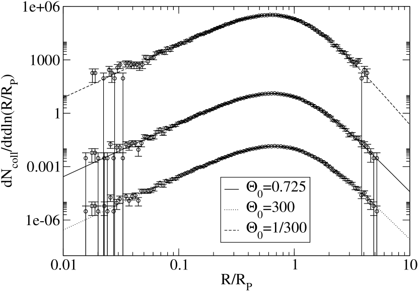
Figure 7.— Comparison of the numerically sampled single-single star collision rate (circles) with the analytical result (lines) for a single-mass Plummer model with $N=10^{6}$ stars, for three different values of the Safronov number ($\Theta_{0}=1/300$, $0.725$, and $300$).

2.4.2 Binary Interactions

All dynamical binary interactions (binary–binary and binary–single) are directly numerically integrated with Fewbody, an efficient computational toolkit for evolving small-$N$ dynamical systems (Fregeau et al., 2004). Fewbody was designed specifically for performing dynamical scattering interactions, and thus it is well-suited for our purposes. See Fregeau et al. (2004) for a detailed description of the code. Note that Fewbody also properly treats physical stellar collisions during binary interactions, using the same criterion for a collision as used in the Monte Carlo code for single–single collisions.

For sampling binary interactions, we use the same technique described above for single–single collisions, but with the cross sections appropriate to binary interactions. For binary–binary interactions, the cross section is given by eq. (9) with $r_{p}=X_{\rm bb}(a_{0}+a_{1})$, where $a_{i}$ are the binary semimajor axes, and $X_{\rm bb}$ is a parameter. $X_{\rm bb}$ must be set large enough so that all binary–binary interactions of interest are followed. Since in this paper we are concerned mainly with the global evolution of clusters, we need only follow most of the energy-generating binary interactions. In principle, one could make $X_{\rm bb}$ arbitrarily large, so as to capture all potentially interesting interactions. The result would be many more weakly-interacting fly-by interactions, which incur an infinitesimal computational cost due to Fewbody’s efficient integration techniques. However, due to the way in which the global Monte Carlo timestep is chosen (see below), time would grind to a halt in our code. Clearly, then, setting $X_{\rm bb}$ is a compromise between capturing all binary interactions of interest (larger $X_{\rm bb}$), and preventing the timestep from becoming unnaturally small (smaller $X_{\rm bb}$). We use $X_{\rm bb}=2$ for the results presented in this paper. For binary–single interactions, we take $r_{p}=X_{\rm bs}a$, where $a$ is the binary semimajor axis, and set $X_{\rm bs}=2$. We find that the values $X_{\rm bs}=X_{\rm bb}=2$ capture almost all the relevant energy-generating binary interactions. Test runs with $X_{\rm bs}=X_{\rm bb}=4$ yield values of $r_{c}/r_{h}$ in the binary burning phase that are statistically consistent with $X_{\rm bs}=X_{\rm bb}=2$ runs for both small and large $f_{b}$.

As we did for single–single collisions, we have performed a calculation of an unevolving Plummer model to test that our code correctly samples the binary interaction rates. In this test, a fraction $f_{b}=0.5$ of the $N=10^{6}$ stars were binaries. The binaries had the same mass as single stars in order to simplify the analytical calculation of the rate. Again, strong interactions were not performed, simply recorded. Since there are two species (binaries and single stars), the interaction rate is given by eq. (11) with an extra factor of $f_{b}$ for binary–single, and $f_{b}^{2}$ for binary–binary. Fig. 8 shows a comparison of the numerically sampled binary interaction rates (circles) with the analytical result (lines) for binary–binary interactions (black) and binary–single (red). The agreement is excellent.

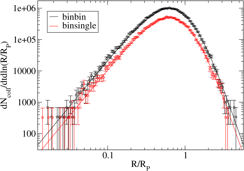
Figure 8.— Comparison of the numerically sampled binary interaction rates (circles) with the analytical result (lines) for binary–binary interactions (black) and binary–single (red) for a single-mass Plummer model with $N=10^{6}$ stars. In this test, binaries had the same mass as single stars. This simplified the analytical calculation of the rate.

Once a binary interaction is deemed to occur, the relative velocity at infinity of the pair is taken to be the current relative velocity of the pair in the cluster (with the angle of each particle’s tangential velocity randomized), and the impact parameter, $b$, of the interaction is chosen uniformly in area out to $b_{\rm max}$ as given in eq. (9). With all parameters of the scattering encounter set, the interaction is numerically integrated with Fewbody until an unambiguous outcome is reached. The outcome products of the interaction are then placed back into the cluster with their resultant internal properties (mass, binary semimajor axis, eccentricity, etc.) and external properties (systemic velocity, etc.).

The only exception to this rule is stable hierarchical triples. These stable triples frequently result from binary–binary interactions (roughly 20% of the time for equal-mass, equal-energy hard binaries; see, e.g., Mikkola, 1983). In principle we could keep the triples in the code, and follow their evolution, allowing them to undergo interactions with other single stars, binaries, and triples (Fewbody can handle all these cases with ease since it is general in $N$). However, for simplicity we currently break triples into a binary and a single star. We do this by allowing the outer member of the triple to just barely escape to infinity, with the inner binary shrinking its orbit to conserve energy in the process. For simplicity, both the single star and binary are given the systemic velocity of the original triple.

Finally, we must discuss one more detail. Since the binary interactions performed with Fewbody are done in a vacuum—in other words, there are no stars other than the ones in the interaction to prevent members of the small-$N$ system from making arbitrarily large excursions—it happens that some binary interactions leave extremely wide binaries (sometimes as wide as the cluster itself) as their outcome products. Clearly this is an unphysical situation, as no binary should ever become larger than the inter-particle separation in a comparable-mass cluster. We therefore break these pathologically wide binaries at the end of each timestep. Our criterion for breaking the binaries is that they have an orbital velocity that is roughly smaller than the local velocity dispersion, since it is this boundary in phase space and not the hard–soft boundary that determines binary lifetime in a cluster (Fregeau et al., 2006). We break the binaries if the orbital speed of their lightest member is less than $X_{\rm hs}\sigma(R)$, where $\sigma(R)$ is the velocity dispersion at position $R$ in the cluster, and $X_{\rm hs}$ is a parameter which we take to be 0.7. We set $X_{\rm hs}<1$ as a safety measure, to ensure that no long-lived binaries are erroneously broken.

2.5. Stellar Evolution

For the mass–radius relationship we adopt an approximate piece-wise fit to the more detailed one used by Freitag et al. (2006b) for $Z=10^{-3}$:

$$R(M)=\begin{cases}0.1R_{\sun}&\quad M/M_{\sun}\leq 0.1\\ R_{\sun}(M/M_{\sun})&\quad 0.1\leq M/M_{\sun}\leq 1\\ R_{\sun}(M/M_{\sun})^{0.57}&\quad 1\leq M/M_{\sun}\leq 120\\ 1.6R_{\sun}(M/M_{\sun})^{0.47}&\quad M/M_{\sun}\geq 120\\ \end{cases}\,.$$ (12)

The first two pieces (up to $M=1\,M_{\sun}$) are based on Chabrier & Baraffe (2000). The next piece is based on Schaller et al. (1992), and the last is from Bond et al. (1984). The fit is a rough approximation to the more exact relationships given in the references listed, but suffices for our purposes since we use it only for determining limits on the properties of the initial binary population (as described below).

2.6. Timestep Evaluation

The timestep in the code should be chosen small enough to resolve the relevant physics (two-body relaxation, collisions, binary interactions, etc.), but not smaller than necessary. We take the timestep to be the minimum of the characteristic timescales for the different physical processes.

For two-body relaxation, we use the standard expression for the characteristic timescale for two species of particles undergoing relaxation to deflect each other by an angle $\theta_{\rm max}$ (Freitag & Benz, 2001):

$$T_{\rm rel}=\frac{\theta_{\rm max}}{\pi/2}\frac{\pi}{32}\frac{v_{\rm rel}^{3}}{\ln(\gamma N)G^{2}n(M_{1}+M_{2})^{2}}\,,$$ (13)

where $v_{\rm rel}$ is the relative speed of the two species, $n$ is the local number density of stars, and $M_{i}$ are the masses of each species of star. The standard expression for the relaxation time comes from setting $\theta_{\rm max}=\pi/2$ (Binney & Tremaine, 1987). We evaluate eq. (13) by a local sliding average as

$$T_{\rm rel}=\frac{\theta_{\rm max}}{\pi/2}\frac{\pi}{32}\frac{\langle v_{\rm rel}\rangle^{3}}{\ln(\gamma N)G^{2}n\langle(M_{1}+M_{2})^{2}\rangle}\,,$$ (14)

yielding $T_{\rm rel}$ as a function of radial position in the cluster. We take the minimum value of $T_{\rm rel}$ for the calculation of the timestep. The minimum most often occurs at the center of the cluster, where the density is the highest. However, it can sometimes happen for clusters with wide mass spectra that the minimum occurs away from the center, due to a massive star in a sea of lighter stars. We adopt $\theta_{\rm max}=1$ for all simulations presented in this paper, which we find to be a good compromise between accuracy and computational speed. The distribution of scattering angles in a typical timestep has a very long tail at large $\theta$, so most super-encounters have a much smaller scattering angle than $\theta_{\rm max}$.

For strong interactions, we evaluate the timescale for each pair of particles neighboring in radius to undergo a strong interaction, by performing an “$n\sigma v$” estimate. This can be written

$$T_{\rm strong}^{-1}=\frac{1}{n}\int d^{3}{\bf v}_{1}d^{3}{\bf v}_{2}f({\bf v}_{1})f({\bf v}_{2})|{\bf v}_{2}-{\bf v}_{1}|S_{\rm strong}\,,$$ (15)

where ${\bf v}_{i}$ is the velocity of star $i$, and $f$ is the velocity distribution function. Assuming a Maxwellian velocity distribution for stars “1” and “2”, the result is

$$T_{\rm strong}^{-1}=4\sqrt{\pi}nr_{p}^{2}\sigma\left(1+\frac{GM}{2r_{p}\sigma^{2}}\right)\,,$$ (16)

where $\sigma$ is the one-dimensional velocity dispersion, and we have substituted eq. (9) for $S_{\rm strong}$. For collisions, we plug in $S_{\rm coll}$ to find

$$T_{\rm coll}^{-1}=16\sqrt{\pi}n_{\rm single}\langle R_{*}^{2}\rangle\sigma\left(1+\frac{G\langle MR_{*}\rangle}{2\sigma^{2}\langle R_{*}^{2}\rangle}\right)\,,$$ (17)

where we explicitly show which quantities we average, and $n_{\rm single}$ is the number density of single stars. Similarly for binary–binary interactions:

$$T_{\rm bb}^{-1}=16\sqrt{\pi}n_{\rm bin}X_{\rm bb}^{2}\langle a^{2}\rangle\sigma\left(1+\frac{G\langle Ma\rangle}{2\sigma^{2}X_{\rm bb}\langle a^{2}\rangle}\right)\,,$$ (18)

and binary–single interactions:

$$T_{\rm bs}^{-1}=4\sqrt{\pi}n_{\rm single}X_{\rm bs}^{2}\langle a^{2}\rangle\sigma\left(1+\frac{G\langle M\rangle\langle a\rangle}{\sigma^{2}X_{\rm bs}\langle a^{2}\rangle}\right)\,,$$ (19)

where $n_{\rm bin}$ is the number density of binaries, and $a$ is the binary semimajor axis.

2.7. Initial Conditions

For our initial cluster models we use both isolated Plummer models and tidally-truncated King models of varying concentration. Our prescription for tidal mass loss is described in detail in Joshi et al. (2001). For models with a mass spectrum or binaries we assume no primordial mass segregation of the heavier components. We use a binary fraction $f_{b}$ from 0 to 1, with the binary fraction defined as $f_{b}=N_{b}/(N_{s}+N_{b})$, where $N_{s}$ is the number of single stars in the cluster, $N_{b}$ is the number of binaries, and $N=N_{s}+N_{b}$.

In assigning the initial properties of the binary population, we start with a cluster of only single stars. We create each binary by randomly choosing a cluster star to be the primary member of the binary, and assigning the secondary mass using a flat distribution for the binary mass ratio $q$ ($dP/dq\propto 1$), truncated at the low end so that the mass of the secondary is not lower than the minimum of the initial mass function. With the masses of both binary members set, the remaining binary properties are set according to one of two different schemes. The first is the scheme that has traditionally been used in numerical modeling of dense stellar systems, in which the binary binding energy $E_{b}$ is distributed uniformly in the logarithm ($dP/dE_{b}\propto E_{b}^{-1}$), with fixed upper and lower limits. As shown in Table 1, we take as limits on the binding energy a few $kT$ on the low end to several hundred $kT$ on the high end, where $kT$ is the thermal energy in the cluster core, evaluated as $\frac{1}{3}\langle mv^{2}\rangle\approx\langle m\rangle\sigma_{c}^{2}$, where $\sigma_{c}$ is the one-dimensional velocity dispersion in the core. With the semimajor axis set by the binding energy, the eccentricity $e$ is set according to the thermal distribution ($dP/de=2e$). The second scheme is a slightly modified version of the first in which the limits on the binding energy and eccentricity are set in a more physical way. The binding energy is still distributed as $dP/dE_{b}\propto E_{b}^{-1}$, but with the upper limit set to the binding energy at a semimajor axis of $5(R_{1}+R_{2})$, where $R_{i}$ are the stellar radii. The lower limit on the binding energy is set to that of a binary whose lightest member has orbital speed $X_{\rm hs}\langle v_{\rm rel}\rangle$, where $X_{\rm hs}$ is as defined in section 2.4.2, and $\langle v_{\rm rel}\rangle$ is the locally averaged relative velocity between objects, taken to be $4\sigma/3\pi$, where $\sigma$ is the local three-dimensional velocity dispersion. The eccentricity is set according to the thermal distribution with an upper limit set by the pericenter distance. Note that when physical limits on $E_{b}$ are used, the resulting cluster simulation is no longer scalable in its length, mass, and time units, since adopting stellar radii sets the physical scale of the system.

3. Example Results and Comparisons

Having verified that our code properly treats two-body relaxation and correctly samples the interaction rates for strong interactions, we now use it study the evolution of more realistic clusters. We first consider clusters of equal-mass stars with primordial binary populations. Note again that for all simulations presented in this paper physical stellar collisions were turned off. The focus of this section is on presenting a few illustrative results in detail, and comparing the results of our newly modified code with those of other codes, as well as the previous version of our code.

Fig. 9 shows the evolution of an isolated Plummer model with $N=10^{5}$ stars, and an initial 3% binary fraction (model pl_n1e5_fb0.03 in Table 1). The top panel shows $M_{b}$, the total mass in binaries bound to the cluster (solid line), and $M$, the total mass of the cluster (dashed line) as a function of time, relative to their initial values. The middle panel shows $E_{\rm bb}$, the cumulative energy generated in binary–binary interactions (solid line) and $E_{\rm bs}$, the cumulative energy generated in binary–single interactions (dashed line) relative to $|E_{c,0}|$, the absolute value of the cluster’s initial mechanical energy. The bottom panel shows the evolution of $r_{c}$, the cluster core radius (solid line), $r_{\rm h,b}$, the half-mass radius of the binaries (dashed line), and $r_{\rm h,s}$, the half-mass radius of single stars (dot-dashed line). The evolution of this model is typical of a cluster with primordial binaries. The core initially shrinks until the central density increases to the point at which energy generation in binary interactions is sufficient to prevent the core from collapsing. The binaries steadily gain binding energy in the subsequent, long-lived binary burning phase. They thus suffer progressively larger kinetic recoil from binary interactions, with the result that eventually the half-mass radius of binaries overtakes the single star half-mass radius. Eventually the binary population is sufficiently depleted in the core that the core collapses, by which point a large fraction of the initial binary population has been depleted ($\sim 90\%$). The binaries are lost either by being disrupted or ejected in binary interactions. From the middle panel it is clear that a significant fraction of energy can be released via binary interactions, in this case of order the initial cluster mechanical energy.

Fig. 10 shows the evolution of the virial ratio and the total cluster energy (cluster mechanical energy plus binary binding energy) for the same model. The virial ratio is conserved to within statistical fluctuations for the duration of the calculation, suggesting that the code is yielding accurate results. The total cluster energy is also conserved relatively well throughout the calculation, at the level of a part in $\sim 10^{4}$, with the largest jump in the energy occurring during the deep core collapse phase. The high degree of conservation of energy and of the virial ratio for this model is typical of all models we present in this paper.

Figure 9.— Evolution of an isolated Plummer model with $N=10^{5}$ stars, and an initial 3% binary fraction (model pl_n1e5_fb0.03 in Table 1). The top panel shows $M_{b}$, the total mass in binaries bound to the cluster (solid line), and $M$, the total mass of the cluster (dashed line) as a function of time, relative to their initial values. The middle panel shows $E_{\rm bb}$, the cumulative energy generated in binary–binary interactions (solid line) and $E_{\rm bs}$, the cumulative energy generated in binary–single interactions (dashed line) relative to $|E_{c,0}|$, the absolute value of the cluster’s initial mechanical energy. The bottom panel shows the evolution of $r_{c}$, the cluster core radius (solid line), $r_{\rm h,b}$, the half-mass radius of the binaries (dashed line), and $r_{\rm h,s}$, the half-mass radius of single stars (dot-dashed line). Time is in initial half-mass relaxation times.

Figure 10.— Evolution of the virial ratio (top panel), and total cluster energy (bottom panel) for model pl_n1e5_fb0.03. The energy plotted here includes not only the mechanical energy of the cluster, but also the binding energy of the binaries. Note the range on the $y$ axis for the energy plot. In this run energy was conserved to a part in $\sim 10^{4}$.

3.1. Comparison with Theory

For the first quantitative test of our results for the quasi steady-state binary burning phase, we appeal to the semi-analytical model of Vesperini & Chernoff (1994). Their model combines the results of binary scattering experiments with an analytical prescription for energy balance in the core, yielding a relationship among the core binary fraction, the properties of the binary population, and the ratio $r_{c}/r_{h}$:

$$\frac{r_{c}}{r_{h}}=\frac{0.1872}{\log_{10}(\gamma N)}\frac{\mu_{\rm bs}\phi_{b}(1-\phi_{b})+\mu_{\rm bb}\phi_{b}^{2}}{(1+\phi_{b})^{4}}\left(\frac{v_{c}}{v_{h}}\right)^{3}\left(\frac{\Gamma}{10}\right)\,,$$ (20)

where $\phi_{b}$ is the core binary fraction, $\mu_{\rm bs}$ and $\mu_{\rm bb}$ are coefficients representing the energy generation rates in binary–single and binary–binary interactions for a given set of binary properties, $v_{c}$ and $v_{h}$ are the core and half-mass velocity dispersions, and $\Gamma$ parameterizes the expansion rate of the core in terms of the half-mass relaxation time. Heggie et al. (2006) have shown that eq. (20) agrees well with the results of $N$-body simulations of $N=4096$ clusters with primordial binaries, with the values $\Gamma=9.4$ and $v_{c}/v_{h}=\sqrt{2}$, which are close to the canonical values of $\Gamma=11.5$ and $v_{c}/v_{h}=\sqrt{2}$ adopted in Vesperini & Chernoff (1994). However, they find that the dependence of $r_{c}/r_{h}$ on $N$ is steeper than eq. (20), in the sense that clusters with $N\gtrsim 10^{3}$ have a systematically smaller value of $r_{c}/r_{h}$ than eq. (20) predicts, with the opposite true for clusters with fewer stars. Extrapolating from the numerical results in Fig. 18 of Heggie et al. (2006), it appears that for $N\sim 10^{5}$ eq. (20) overestimates $r_{c}/r_{h}$ by a factor of $\approx 2$ for the values $\Gamma=10$ and $v_{c}/v_{h}=\sqrt{2}$.

To test the agreement between our code and eq. (20), we have performed several cluster simulations of varying initial binary fraction and measured the core radius and binary fraction after core stabilization. The details of the models (pl_n3e5_fb0.01_kt through pl_n3e5_fb0.60_kt) are given in Table 1. Fig. 11 shows $r_{c}/r_{h}$ vs. core binary fraction $\phi_{b}$ for the simulations, compared with eq. (20). Each set of points (shown as circles and triangles, alternating) represents a simulation with a different initial binary fraction. Each point is determined by averaging over a time window of width $\Delta t=t_{\rm rh}$ from the point of core stabilization until several $t_{\rm rh}$ later. The solid line shows the theoretical model with the standard values $\Gamma=10$ and $v_{c}/v_{h}=\sqrt{2}$ for $E_{b}=10$–$100\,kT$. The agreement between our code and the semi-analytical model is quite satisfactory for $\phi_{b}\lesssim 0.5$. Above this value the two differ by up to a factor of $\sim 2$, with our code yielding $r_{c}/r_{h}$ values smaller than predicted by theory. We believe the apparent discrepancy is due to the destruction in binary–binary interactions of the wider binaries in the initial binary distribution, the rate of which increases with increasing binary fraction. For reference, the theoretical curve for a narrower range of binary binding energies ($E_{b}=25$–$100\,kT$) is shown in the dashed line.

Figure 11.— The quantity $r_{c}/r_{h}$ vs. core binary fraction $\phi_{b}$ for simulations pl_n3e5_fb0.01_kt through pl_n3e5_fb0.60_kt, compared with the semi-analytical model of Vesperini & Chernoff (1994). Each set of points (shown as circles and triangles, alternating) represents a simulation with a different initial binary fraction (from left to right): $f_{b}=0.01$, $0.02$, $0.04$, $0.08$, $0.15$, $0.3$, and $0.6$. Each point is determined by averaging over a time window of width $\Delta t=t_{\rm rh}$ from the point of core stabilization until several $t_{\rm rh}$ later. The solid line shows the theoretical model with the standard values $\Gamma=10$ and $v_{c}/v_{h}=\sqrt{2}$ for $E_{b}=10$–$100\,kT$, while the dashed line shows the theoretical model with $E_{b}=25$–$100\,kT$ to reflect the depletion of the widest binaries due to binary–binary interactions.

Finally, we mention the issue of post-collapse, gravothermal core oscillations. Gravothermal oscillations are driven by the gravothermal instability (essentially the negative heat capacity of gravitational systems, which causes heat to flow from cold to hot in a runaway fashion). At any given time during deep core collapse, the temperature profile is a monotonically decreasing function of $r$, with the central temperature steadily increasing as a function of time. At some point during the collapse, a binary scattering interaction occurs, producing a small amount of energy in the core and cooling it, creating a temperature inversion. Once the temperature inversion is established, the gravothermal instability takes over and drives the subsequent core expansion. There are several hallmarks of gravothermal oscillations. One is, of course, a temperature inversion in the cluster core at the point when the core begins to rebound. Another is that the expansion phase is not driven by energy generation in binaries. Yet another is the presence of loops in a phase space diagram of the cluster core properties (Makino, 1996; Heggie et al., 2006). In Paper III we demonstrated the gravothermal nature of the core oscillations produced by our code by displaying the temperature inversion in the core. As in Paper III, cluster models evolved with our newly modified code undergo core oscillations after core collapse. Preliminary tests show loops in phase space, but with the wrong directional sense, implying that the oscillations we now see are not gravothermal in nature. Since we are concerned only with pre-deep core collapse evolution in this paper, we postpone for future work a more detailed analysis of the core oscillations produced by our newly modified code.

3.2. Comparison with Previous Numerical Work

The amount of numerical work reported on clusters with primordial binaries has grown considerably since the work of Gao et al. (1991), who used a multimass Fokker-Planck code coupled with a recipes-based treatment of binary interactions. In Paper III, we used a Monte Carlo code coupled with recipes for binary interactions. Giersz & Spurzem (2003) used a hybrid code, which treated single stars via a gas dynamical method and binaries via Monte Carlo, and performed direct numerical integration of binary interactions. Heggie et al. (2006) and Trenti et al. (2006b) performed direct $N$-body simulations. And as described in the preceding sections, in this paper we use a Monte Carlo method coupled with direct numerical integration of binary interactions. In this section we compare the results from our code with those from all the methods just listed.

Figure 12.— Evolution of the “Gao, et al.” model: an isolated Plummer model with $N=10^{5}$ objects, equal-mass stars, and 10% binaries (model T4). Quantities plotted are the same as in Fig. 9.

A standard model has emerged in the business of simulating the evolution of clusters containing primordial binaries. The “Gao, et al.” model is an isolated Plummer model with equal-mass stars and 10% binaries, with the binary binding energy distributed uniformly in the logarithm from $3$ to $400kT$, and with the binary eccentricity distributed according to the thermal distribution. Since this model has been treated by all the previous work cited above, we use it as a basis for comparison. Fig. 12 shows the evolution of this model (T4 in Table 1). Fig. 13 shows the evolution of the ratio $r_{c}/r_{h}$. Although we did not integrate our model to deep core collapse, which occurs at $t\approx 50t_{\rm rh}$ in Gao et al. (1991) and $t\approx 130t_{\rm rh}$ in Heggie et al. (2006), there are still ample results for comparison. Comparing with Fig. 1 of Gao et al. (1991), the timescale of the initial core contraction we find is nearly identical at $\approx 11t_{\rm rh}$. This is the same timescale found by Heggie et al. (2006) in their Fig. 2 and Giersz & Spurzem (2003) in their Fig. 4, although in the latter case the comparison is less meaningful since their results show no long-lived binary burning phase. It is also similar to the result of Paper III in Fig. 4, although in that paper we found a slightly shorter timescale.

Turning now to the size of the core radius during the binary burning phase, we find $r_{c}\approx 0.07$ in $N$-body units. The model of Gao et al. (1991) shows a smaller core size, with $r_{c}\approx 0.05$ in $N$-body units (note that the unit of length in their plot is $3\pi/16$ in $N$-body units). This is somewhat expected, since the code of Gao et al. (1991) predicts a smaller core than the semi-analytical theory (Heggie et al., 2006). The recipes-based model of Paper III shows a much larger core, with $r_{c}\approx 0.2$. This is not surprising, since recipes tend to overestimate the energy generation rate in binary interactions (Fregeau et al., 2003; Giersz & Spurzem, 2003; Fregeau et al., 2005). Although the model of Giersz & Spurzem (2003) does not show a long-lived binary burning phase, there is a subtle hint of a short-lived one with $r_{c}\approx 0.2$. This is also much larger than the value we find. Comparing our Fig. 13 with Fig. 2 of Heggie et al. (2006), we see qualitatively very similar behavior in the two calculations, with $r_{c}/r_{h}$ abruptly slowing its contraction at $t\approx 11t_{\rm rh}$ and steadily decreasing thereafter. At the start of the binary-burning phase, Heggie et al. (2006) find $r_{c}/r_{h}\approx 0.06$, just as we do. If the scaling of $r_{c}/r_{h}$ with $N$ in Heggie et al. (2006) can be extrapolated out to $N\sim 10^{5}$ as described in section 3.1, then this agreement is somewhat surprising. In terms of the structural parameters during the binary burning phase (which, as the longest-lived evolutionary phase in the life of a cluster is the most observationally relevant), as well as the timescale to reach it, our code appears to agree well with $N$-body, slightly less well with the Fokker-Planck code, and much less well with the two other approximate codes.

Figure 13.— Evolution of $r_{c}/r_{h}$ for model T4. The solid line uses the Casertano & Hut (1985) technique to measure the core radius, while the dotted line uses the standard Spitzer (1987) definition.

We can also compare the mass in binaries (or, equivalently, number) as a function of time. At the somewhat arbitrary time of $40t_{\rm rh}$, we find $M_{b}/M_{b,0}\approx 0.35$. Gao et al. (1991) find a value of 0.41, while Heggie et al. (2006) find a value of 0.36. In Paper III we found a value of 0.35. All these methods appear to agree very well on the average rate that binaries are lost (either ejected or disrupted in binary interactions) up to $40t_{\rm rh}$, although the agreement with Paper III is probably fortuitous given the disagreement in the structural parameters.

Comparing an isolated cluster model tests in combination how well our code treats two-body relaxation, mass segregation, and the various aspects of binary burning. Having shown that our code agrees well with the “exact” method of $N$-body, one can be fairly confident that our code treats these processes relatively accurately. However, since all dense star clusters are tidally truncated to some degree, it is still useful to consider how well our code treats the physics of tidal stripping. As described in Joshi et al. (2001), we use a cutoff radius criterion to determine whether a star has been stripped from the cluster. This is in contrast to the more accurate technique of including the tidal field in the equations of motion (which is not possible for the Monte Carlo method). Trenti et al. (2006b) have compared the two tidal stripping methods by performing $N$-body simulations of $N\sim 10^{4}$ clusters with primordial binaries, and have found that models using a tidal cutoff tend to survive longer before disrupting (up to a factor of $\sim 2$, although it’s not clear how this factor scales with $N$), and have a larger core radius (again, up to a factor of $\sim 2$), than models with a tidal field. We will keep this in mind when presenting results below. For now we compare two current simulations with the tidal cutoff models of Trenti et al. (2006b), and with the previous version of our code. Figs. 14 and 15 show the evolution of models w3_n1e5_fb0.1 and w7_n1e5_fb0.1, respectively. Comparing the first with Fig. 13 in Paper III, we see that although both models reach disruption, our new results are qualitatively different in behavior, yielding what appears to be a binary burning phase from $9t_{\rm rh}$ to disruption, while the old result shows no such phase. Aside from this difference, the quantitative evolution of the structural radii, the total cluster and binary mass, and the disruption timescale appear to be very similar between the two models. Comparing with Fig. 16 of Trenti et al. (2006b), we find similar qualitative behavior, with a hint of a binary burning phase in their results starting at roughly the same time, similar evolution of the structural radii, and both models resulting in disruption at $\sim 12$–$14t_{\rm rh}$. Our model seems to predict a smaller core radius, by a factor of $\sim 2$. Note that Trenti et al. (2006b) use the Spitzer definition of the core radius, which they find with their code to yield a value $\sim 20\%$ larger than the density-weighted averaging method.

Moving on to the $W_{0}=7$ model, we find similar qualitative behavior but shorter disruption times than both Fig. 10 in Paper III and Trenti et al. (2006b) in their Fig. 17. The recipes-based model of Paper III predicts a much larger core radius in the binary burning phase than our current model. This is due to the fact that the recipes used in that calculation tend to overestimate the rate of energy generation in binary burning. The agreement with Trenti et al. (2006b) is better, with our core radius being only $\sim 20\%$ smaller than the $N$-body result. Looking at the evolution of $M$ and $M_{b}$, our model appears to exhibit very similar behavior to the $N$-body model.

In general, our new code yields much improved agreement with the $N$-body results reported in the literature, for both isolated and tidally-truncated models, but yields some results that differ significantly from other approximate methods. Notably, the direct integration of binary interactions reduces their energy generation rate relative to the simple recipes used in Paper III, and yields smaller core radii. This was evident to some degree in Paper III, in which the discrepancy was illustrated for binary–single interactions. Below we compare our new results with observations and discuss the implications.

Figure 14.— Evolution of model THH3. Quantities plotted are the same as in Fig. 9.

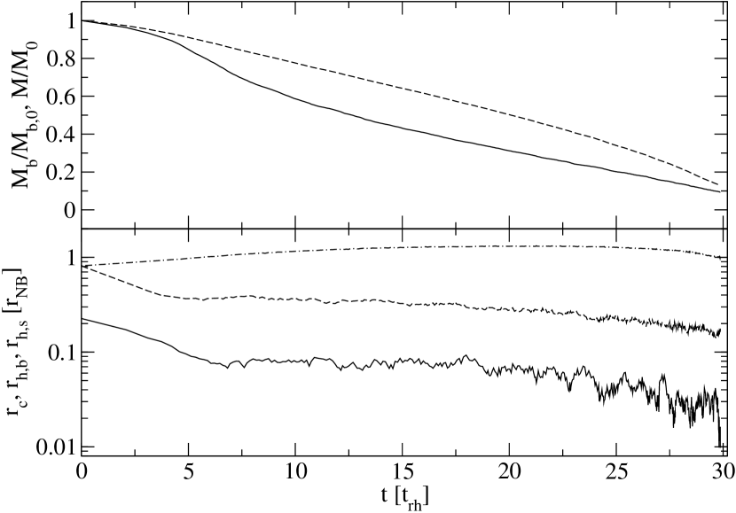
Figure 15.— Evolution of model THH7. Quantities plotted are the same as in Fig. 9.

4. Results and Comparison with Observations

Figure 16.— Evolution of model w11_n1e5_fb0.3. Quantities plotted are the same as in Fig. 9.

Figure 17.— Evolution of $r_{c}/r_{h}$ (dashed line), total cluster binary fraction $f_{b}$ (dot-dashed line), core binary fraction $f_{\rm b,c}$ (dotted line), and concentration $c$ (solid line) for model w11_n1e5_fb0.3.

Figure 18.— Evolution of $c$ and $r_{c}/r_{h}$ for $W_{0}=3$, $7$, and $11$ models with $f_{b}=0.1$ (solid lines) and $f_{b}=0.3$ (dashed lines). Note the “universal” behavior, with the initially more centrally concentrated models ($W_{0}=11$) expanding and the less centrally concentrated models ($W_{0}=3$ and $7$) contracting to common values of $r_{c}/r_{h}$ and $c$.

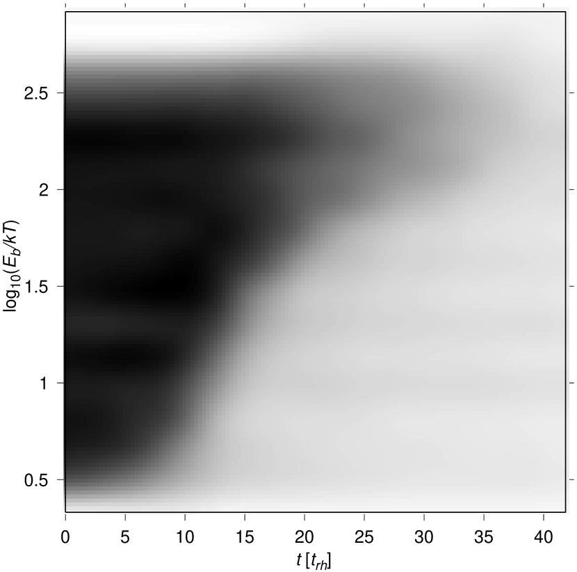
Figure 19.— Evolution of the binary binding energy distribution for model T5. The distribution starts off uniform in $\log E_{b}$ from 3 to 400 $kT$. As the cluster evolves the central velocity dispersion increases, moving the hard–soft boundary to larger $E_{b}$ and destroying the wider binaries. Near core collapse ($\sim 40t_{\rm rh}$), only a small collection of relatively tight binaries ($E_{b}\sim 300\,kT$) remains.

In addition to displaying the initial conditions for all models simulated for this paper, Table 1 gives several important measured quantities for each simulation. The first is the core stabilization time, $t_{\rm cs}$, at which the core radius stabilizes (i.e., the start of the binary-burning phase) after the initial contraction or expansion. Note that some authors denote this as the core collapse time when discussing clusters with primordial binaries. The second is the time of the first deep core collapse, $t_{\rm cc}$, which, for models with binaries, represents the time at which the binary population is nearly depleted in the core. The next is the disruption time, $t_{\rm dis}$, for models which are tidally truncated. The next is $r_{c}/r_{h}$, the ratio of the core to half-mass radius averaged over $1\,t_{\rm rh}$ after $t_{\rm cs}$. Finally, $c=\log_{10}(r_{t}/r_{c})$ is the concentration parameter averaged over the same time period. The evolution of several of the models in the table has been shown graphically in the preceding figures. The behavior of the remaining models is similar to the ones already shown, with the relevant timescales and structural parameters appropriately modified. The only exceptions are the high concentration King models, which undergo an initial phase of core expansion (instead of contraction) due to their initially very dense state. Fig. 16 displays the evolution of such a model, model w11_n1e5_fb0.3. For reference we have plotted the time evolution of the measured quantities $r_{c}/r_{h}$ and $c$ in Fig. 17, along with the the total cluster binary fraction $f_{b}$ and the core binary fraction $f_{\rm b,c}$.

Fig. 18 shows the evolution of $c$ and $r_{c}/r_{h}$ for $W_{0}=3$, $7$, and $11$ models with $f_{b}=0.1$ (solid lines) and $f_{b}=0.3$ (dashed lines). Of note is the “universal” behavior displayed by the models, in which the initially more centrally concentrated models ($W_{0}=11$) expand and the less centrally concentrated models ($W_{0}=3$ and $7$) contract to common values of $r_{c}/r_{h}$ and $c$. This is the same behavior found previously in the literature, in Paper III and Trenti et al. (2006b) in their Fig. 8, although in the latter case they find systematically larger values of $r_{c}/r_{h}$ and smaller values of $c$ (as described above). For reference we also show in Fig. 19 the evolution of the binary binding energy distribution for model T5. The softest binaries begin to be destroyed (by ejection or disruption in binary interactions) on the approach to core stabilization. As the cluster evolves the central velocity dispersion increases, moving the hard–soft boundary to larger $E_{b}$ and destroying the wider binaries. Near core collapse ($\sim 40t_{\rm rh}$), only a small collection of relatively tight binaries ($E_{b}\sim 300\,kT$) remains. The evolution of the binary population in $E_{b}$–$r$ space is qualitatively similar to what’s shown in Fig. 15 of Paper III, with the softer binaries first being destroyed in the core, and the harder binaries becoming even harder and more centrally concentrated with time.

There are several trends apparent in the data presented in Table 1. For fixed initial cluster structure, as $f_{b}$ is increased from zero, $t_{\rm cs}$ decreases from the value of $t_{\rm cc}$ at $f_{b}=0$, reaches a minimum around $f_{b}\sim 0.2$, then increases back to approximately its $f_{b}=0$ value for $f_{b}=1$. This dip is due to the fact that in the initial core contraction or expansion phase, binaries act primarily as a second, heavier star species, hastening cluster energy transport via mass segregation. Looking at the deep core collapse times, another clear trend is that $t_{\rm cc}$ increases dramatically as $f_{b}$ is increased. This trend is most striking in the isolated Plummer models, with merely $f_{b}\approx 0.03$ being enough to double the deep core collapse time, and $f_{b}=1$ increasing it by a factor of at least 7 (model T4). The physical explanation is, of course, that the lifetime of the binary-burning phase increases with the amount of fuel available, in analogy to hydrogen-burning in main-sequence stars. Looking more carefully at the tidally-truncated King models, we see that the presence of binaries tends to drive these clusters to complete tidal disruption. The minimum of $t_{\rm dis}$ occurs somewhere in the range $0.1\lesssim f_{b}\lesssim 1$. This is not surprising, since the maximum of $r_{c}/r_{h}$ occurs at $f_{b}\approx 0.4$ (see Fig. 11), implying that the cluster is the most distended for this value of $f_{b}$. Moving now to the cluster structural parameters, we see that there is relatively little variation in $r_{c}/r_{h}$ and $c$ over the wide range of cluster initial profiles and binary fractions considered, with $r_{c}/r_{h}$ ranging from $\sim 0.05$ for Plummer or $W_{0}\sim 7$ King models with low $f_{b}$, to $\sim 0.1$ for larger $W_{0}$ King models with $f_{b}\sim 1$. The concentration parameter shows a similarly small amount of variation, peaking at $\sim 2.1$ for $W_{0}\sim 7$ and low binary fraction, and falling to $\sim 1.7$ for larger $W_{0}$ and larger binary fraction. As expected, a larger $f_{b}$ leads to a smaller $c$, since the core radius generally increases with binary fraction. Another trend is evident when comparing single-mass models with models incorporating a more realistic mass spectrum (Salpeter from $0.2$–$1.2\,M_{\sun}$): models with a mass spectrum tend to have a slightly smaller $r_{c}/r_{h}$, and show more variation of $c$ with $W_{0}$.

Although our cluster evolution models are rather simplified (since they do not include single- or binary-star stellar evolution, or collisions), it is still useful to compare the predicted structural parameters with observations. In Paper III we compared $r_{c}/r_{h}$ and $c$ from simulations using the previous version of our Monte Carlo code (which includes recipes for binary interactions instead of dynamical integrations), with observations for the Galactic globular clusters. There we found promising agreement, with $r_{c}/r_{h}$ from the simulations falling generally in the low $r_{c}/r_{h}$ region of the observed distribution for non-core collapsed clusters, which extends from $\sim 0.1$ to $\sim 1$ with a peak at $\sim 0.5$. And similarly for $c$, falling in the high $c$ region of the observed distribution for non-core collapsed clusters, which extends from $\sim 0.5$ to $\sim 2.5$ with a peak at $\sim 1.5$. However, as described above, we find systematically smaller values for $r_{c}/r_{h}$ than in Paper III by a factor of up to $\sim 10$, as well as systematically larger values for $c$ by $\sim 0.5$. The improved treatment of binary interactions in our code has shifted our predictions for $r_{c}/r_{h}$ and $c$ outside the observed ranges for non-core collapsed clusters, now yielding agreement only with the roughly 10% of Galactic globular clusters that are classified observationally as core collapsed.

A globular cluster of comparable mass stars with $f_{b}\gtrsim 0.03$ viewed at a random time during its life has a greater than 50% chance of being found in the quasi-steady state binary burning phase. When one considers that globulars are likely born with significant binary fractions (Hut et al., 1992; Ivanova et al., 2005), and that we are currently observing the Galactic globular clusters at a late stage in their evolution, the vast majority of observed clusters should currently be in the binary-burning phase. The most obvious interpretation of the observational data is that most Galactic globular clusters are currently in the binary-burning phase, and the roughly 10% classified as core-collapsed are within a small time window around a deep core collapse phase. The disagreement between simulations and observations for the structural parameters of the non core-collapsed clusters, then, suggests one of at least two possibilities: 1) the Galactic globular clusters do not start within the volume in parameter space of initial conditions we have considered here; or 2) there are additional physical processes at work in clusters, yielding larger cores. If clusters are born with $W_{0}\gtrsim 11$ and $f_{b}\lesssim 1$, extrapolation of our results suggests that simulations may then agree with the observations of non-core collapsed clusters, implying possibility (1) may be correct. However, a cluster with $W_{0}\gtrsim 11$ is likely to have a short enough central relaxation time that a runaway stellar collision will occur, creating an intermediate mass black hole (IMBH) early in the cluster’s lifetime (Freitag et al., 2006a). This is intriguing, since clusters with central IMBHs typically have significantly larger values of $r_{c}/r_{h}$ than clusters without (Trenti et al., 2006a). We have not included in our simulations any form of stellar evolution (for single stars or binaries), or physical stellar collisions. Single star evolution tends to heat a cluster early in its lifetime via wind-driven mass loss and supernovae explosions, causing the cluster and its core to expand. However, this effect is most pronounced only early in the lifetime of a star cluster ($\lesssim 1\,{\rm Gyr}$). The effects of binary stellar evolution are less obvious, since it is a rather complicated process. However, the simulations of Ivanova et al. (2005) suggest that the binary fraction in the core quickly drops to relatively small values ($\lesssim 20\%$), and that binary stellar evolution tends to destroy tight binaries. The net result is likely to be a smaller equilibrium value of $r_{c}/r_{h}$ (Vesperini & Chernoff, 1994) than with no binary stellar evolution, suggesting that possibility (2) is less likely. A refined quantitative study combining the results of Ivanova et al. (2005) and Vesperini & Chernoff (1994) would more clearly elucidate this effect.

The effect of direct single–single star collisions in young dense clusters is to dissipate orbital energy and drive core collapse (Freitag et al., 2006a). For clusters in which stellar merger products have had time to evolve and lose mass through accelerated stellar evolution, the net result may be to heat the core (Lee, 1987). The degree to which this process operates in Galactic globular clusters is unclear, however. The effect of stellar collisions during binary interactions is generally to reduce the efficiency of binary burning (Hut & Inagaki, 1985; McMillan, 1986; Goodman & Hernquist, 1991). This is because a merger product resulting from a star–star collision typically has significantly more internal energy (potential and rotational) than the sum of the merging stars’ internal energies. Thus when a collision occurs during a binary dynamical interaction, effectively some of the binding energy of the binary is converted into stellar binding energy, decreasing the efficiency of binary burning. In other words, energy that had previously been available to be converted into kinetic energy through binary interactions is no longer available, tied up in the stars. The result should be a decreased value of $r_{c}/r_{h}$ in the binary-burning phase relative to the case of point-mass binary dynamics, implying that possibility (2) is less likely. As with binary stellar evolution, however, a more detailed simulation which studies the effects of collisions in an evolving model should be performed to quantify the effect.

5. Summary and Conclusions

In this paper we have described our new Monte Carlo evolution code and used it to perform a large set of cluster evolution simulations, which we compared with previous results in the literature, as well as observations of Galactic globular clusters.

In section 2 we described our new code in detail, including the implementation of direct integration of binary scattering interactions and star–star physical collisions, and the fundamental modifications we have made to the core Monte Carlo method. We performed several test calculations with the code, finding that it reproduces well several standard results. It yields a core collapse time of $\approx 18\,t_{\rm rh}$ for an isolated Plummer model, in good agreement with results in the literature. It also produces an $r^{-2.3}$ density profile during the late stages of core collapse, in good agreement with the theoretical expectation. We also performed comparisons of clusters with increasingly wide mass spectra with $N$-body, finding that for moderately wide mass spectra ($1$ to $10\,M_{\sun}$) the agreement with $N$-body is satisfactory, but for very wide mass spectra ($0.2$ to $120\,M_{\sun}$) the agreement is not as good. In particular, for such wide mass spectra, our Monte Carlo code tends to overestimate the mass segregation timescale at early times, and underestimate it at later times. The sense of the disagreement is the same as found by Freitag et al. (2006b) with their Monte Carlo code.

In section 3 we displayed a few example results and compared with theory and previous numerical calculations in the literature. We found that the code conserves energy well over the long timescales of our runs. We compared our predicted values of $r_{c}/r_{h}$ during the quasi-steady state binary burning phase with the semi-analytical work of Vesperini & Chernoff (1994), finding good agreement. We compared our results with previous numerical results in the literature for isolated and tidally-truncated cluster models, finding excellent agreement with $N$-body calculations. There are much larger discrepancies with the other approximate methods (Fokker-Planck and other Monte Carlo codes), which is to be expected, since most used recipes for binary interactions, which are known to overestimate the energy generation rate in binaries.

In section 4 we surveyed the results from all our simulations, and compared with observations. Our models cover a large range in parameter space, using Plummer and King models with $W_{0}=3$ to 11 for the initial cluster profile, and with initial binary fractions from 0 to 1. The resulting structural parameters in the binary burning phase span a remarkably small range, with $r_{c}/r_{h}$ varying from 0.03 to 0.12, and $c$ varying from 1.7 to 2.4. Our results for these structural parameters are distinctly different from the results found with the previous version of our code (which used recipes for binary interactions), with $r_{c}/r_{h}$ now smaller than what we found in Paper III by a factor of up to $\sim 10$, and with $c$ larger by $\sim 0.5$. Although our new results agree much better with $N$-body calculations, they unfortunately agree much less well than in Paper III with the observations. The disagreement implies one of at least two possibilities. It may be that the initial conditions for Galactic globular clusters are outside the range of initial conditions we have sampled in this work. Extrapolation of our results suggests that clusters with $W_{0}\gtrsim 11$ and $f_{b}\lesssim 1$ may match the observations. This is intriguing since a cluster with $W_{0}\gtrsim 11$ will likely form an IMBH early in its lifetime via a collisional runaway, and clusters with central IMBHs are known to have larger values of $r_{c}/r_{h}$ (Freitag et al., 2006a; Trenti et al., 2006a). Alternatively, stellar evolution and collisions, which are not included in the simulations in this paper, could possibly explain the disagreement. However, it appears that the effect of these processes should act in the opposite sense of ameliorating the disagreement with observations. More detailed simulations including the effects of single- and binary-star evolution and physical collisions should be performed to test this.

Table 1Parameters and measured quantities for all model simulations presented in this paper.

name	$N$	profile	$r_{\rm NB}/{\rm pc}$	$f(M/M_{\sun})$	$f_{b}$	$f(E_{b}/kT)$	$t_{\rm cs}/t_{\rm rh}$	$t_{\rm cc}/t_{\rm rh}$	$t_{\rm dis}/t_{\rm rh}$	$r_{c}/r_{h}$	$c$
T1	$5\times 10^{5}$	Plum.	$1.02$	$\propto\delta(M-1)$	0	$\cdots$	$\cdots$	17.6	$\cdots$	$\cdots$	$\cdots$
T2	$10^{6}$	Plum.	$0.58$	Kroup., $0.1$–$10$	0	$\cdots$	$\cdots$	0.54	$\cdots$	$\cdots$	$\cdots$
T3	$1.25\times 10^{6}$	Plum.	$0.60$	Salp., $0.2$–$120$	0	$\cdots$	$\cdots$	0.067	$\cdots$	$\cdots$	$\cdots$
T4	$10^{5}$	Plum.	$7.49$	$\propto\delta(M-1)$	0.1	$\propto E_{b}^{-1}$, $3$–$400$	11	$>128$	$\cdots$	0.06	$\cdots$
T5	$10^{5}$	Plum.	$7.33$	$\propto\delta(M-1)$	0.03	$\propto E_{b}^{-1}$, $3$–$400$	14	$42$	$\cdots$	0.06	$\cdots$
THH3	$10^{5}$	$W_{0}=3$	$7.49$	$\propto\delta(M-1)$	0.1	$\propto E_{b}^{-1}$, $3$–$400$	$9.4$	$11.8$	$>11.8$	$0.07$	$1.8$
THH7	$10^{5}$	$W_{0}=7$	$7.49$	$\propto\delta(M-1)$	0.1	$\propto E_{b}^{-1}$, $3$–$400$	$6.7$	$29.8$	$>29.8$	$0.08$	$1.9$
pl_n3e5_fb0.01_kt	$3\times 10^{5}$	Plum.	$5.44$	$\propto\delta(M-1)$	0.01	$\propto E_{b}^{-1}$, $10$–$100$	$16.3$	$>23$	$\cdots$	$0.04$	$\cdots$
pl_n3e5_fb0.02_kt	$3\times 10^{5}$	Plum.	$5.46$	$\propto\delta(M-1)$	0.02	$\propto E_{b}^{-1}$, $10$–$100$	$14.2$	$>23$	$\cdots$	$0.06$	$\cdots$
pl_n3e5_fb0.04_kt	$3\times 10^{5}$	Plum.	$5.49$	$\propto\delta(M-1)$	0.04	$\propto E_{b}^{-1}$, $10$–$100$	$12.5$	$>23$	$\cdots$	$0.07$	$\cdots$
pl_n3e5_fb0.08_kt	$3\times 10^{5}$	Plum.	$5.56$	$\propto\delta(M-1)$	0.08	$\propto E_{b}^{-1}$, $10$–$100$	$11.0$	$>23$	$\cdots$	$0.07$	$\cdots$
pl_n3e5_fb0.15_kt	$3\times 10^{5}$	Plum.	$5.68$	$\propto\delta(M-1)$	0.15	$\propto E_{b}^{-1}$, $10$–$100$	$10.4$	$>23$	$\cdots$	$0.06$	$\cdots$
pl_n3e5_fb0.30_kt	$3\times 10^{5}$	Plum.	$5.92$	$\propto\delta(M-1)$	0.3	$\propto E_{b}^{-1}$, $10$–$100$	$12.6$	$>23$	$\cdots$	$0.06$	$\cdots$
pl_n3e5_fb0.60_kt	$3\times 10^{5}$	Plum.	$6.34$	$\propto\delta(M-1)$	0.6	$\propto E_{b}^{-1}$, $10$–$100$	$17.5$	$>23$	$\cdots$	$0.05$	$\cdots$
pl_n1e5_fb0	$10^{5}$	Plum.	$7.25$	$\propto\delta(M-1)$	0	$\cdots$	$\cdots$	$17.6$	$\cdots$	$\cdots$	$\cdots$
pl_n1e5_fb0.03	$10^{5}$	Plum.	$7.33$	$\propto\delta(M-1)$	0.03	$\propto E_{b}^{-1}$, phys.	$15$	$33.3$	$\cdots$	$0.05$	$\cdots$
pl_n1e5_fb0.1	$10^{5}$	Plum.	$7.49$	$\propto\delta(M-1)$	0.1	$\propto E_{b}^{-1}$, phys.	$10$	$>28$	$\cdots$	$0.07$	$\cdots$
pl_n1e5_fb0.3	$10^{5}$	Plum.	$7.92$	$\propto\delta(M-1)$	0.3	$\propto E_{b}^{-1}$, phys.	$12$	$>32$	$\cdots$	$0.06$	$\cdots$
pl_n1e5_fb1	$10^{5}$	Plum.	$9.14$	$\propto\delta(M-1)$	1	$\propto E_{b}^{-1}$, phys.	$18$	$>22$	$\cdots$	$0.07$	$\cdots$
w3_n1e5_fb0	$10^{5}$	$W_{0}=3$	$7.25$	$\propto\delta(M-1)$	0	$\cdots$	$\cdots$	$13.7$	$>13.7$	$\cdots$	$\cdots$
w3_n1e5_fb0.03	$10^{5}$	$W_{0}=3$	$7.33$	$\propto\delta(M-1)$	0.03	$\propto E_{b}^{-1}$, phys.	$11$	$13.8$	$13.8$	$0.06$	$1.9$
w3_n1e5_fb0.1	$10^{5}$	$W_{0}=3$	$7.49$	$\propto\delta(M-1)$	0.1	$\propto E_{b}^{-1}$, phys.	$9$	$12.2$	$12.2$	$0.08$	$1.8$
w3_n1e5_fb0.3	$10^{5}$	$W_{0}=3$	$7.92$	$\propto\delta(M-1)$	0.3	$\propto E_{b}^{-1}$, phys.	$10$	$11.5$	$11.5$	$0.06$	$1.8$
w3_n1e5_fb1	$10^{5}$	$W_{0}=3$	$9.14$	$\propto\delta(M-1)$	1	$\propto E_{b}^{-1}$, phys.	$14$	$16.3$	$16.3$	$0.06$	$1.9$
w7_n1e5_fb0	$10^{5}$	$W_{0}=7$	$7.25$	$\propto\delta(M-1)$	0	$\cdots$	$\cdots$	$11.1$	$>11.1$	$\cdots$	$\cdots$
w7_n1e5_fb0.03	$10^{5}$	$W_{0}=7$	$7.33$	$\propto\delta(M-1)$	0.03	$\propto E_{b}^{-1}$, phys.	$10$	$19.9$	$>19.9$	$0.05$	$2.1$
w7_n1e5_fb0.1	$10^{5}$	$W_{0}=7$	$7.49$	$\propto\delta(M-1)$	0.1	$\propto E_{b}^{-1}$, phys.	$7$	$30.3$	$>30.3$	$0.07$	$2.0$
w7_n1e5_fb0.3	$10^{5}$	$W_{0}=7$	$7.92$	$\propto\delta(M-1)$	0.3	$\propto E_{b}^{-1}$, phys.	$7$	$29.0$	$>29.0$	$0.06$	$2.0$
w7_n1e5_fb1	$10^{5}$	$W_{0}=7$	$9.14$	$\propto\delta(M-1)$	1	$\propto E_{b}^{-1}$, phys.	$14$	$38.7$	$38.7$	$0.07$	$1.9$
w11_n1e5_fb0	$10^{5}$	$W_{0}=11$	$7.25$	$\propto\delta(M-1)$	0	$\cdots$	$\cdots$	$1.0$	$>1.0$	$\cdots$	$\cdots$
w11_n1e5_fb0.03	$10^{5}$	$W_{0}=11$	$7.33$	$\propto\delta(M-1)$	0.03	$\propto E_{b}^{-1}$, phys.	$2$	$13.0$	$>13.0$	$0.07$	$2.0$
w11_n1e5_fb0.1	$10^{5}$	$W_{0}=11$	$7.49$	$\propto\delta(M-1)$	0.1	$\propto E_{b}^{-1}$, phys.	$1$	$>3.6$	$>3.6$	$0.09$	$1.9$
w11_n1e5_fb0.3	$10^{5}$	$W_{0}=11$	$7.92$	$\propto\delta(M-1)$	0.3	$\propto E_{b}^{-1}$, phys.	$1$	$>2.9$	$>2.9$	$0.09$	$1.8$
w11_n1e5_fb1	$10^{5}$	$W_{0}=11$	$9.14$	$\propto\delta(M-1)$	1	$\propto E_{b}^{-1}$, phys.	$2$	$25.0$	$25.0$	$0.12$	$1.7$
pl_n1e5_s_fb0	$10^{5}$	Plum.	$5.05$	Salp., $0.2$–$1.2$	0	$\cdots$	$\cdots$	4.9	$\cdots$	$\cdots$	$\cdots$
pl_n1e5_s_fb0.03	$10^{5}$	Plum.	$5.09$	Salp., $0.2$–$1.2$	0.03	$\propto E_{b}^{-1}$, phys.	$5$	$12.7$	$\cdots$	$0.03$	$\cdots$
pl_n1e5_s_fb0.1	$10^{5}$	Plum.	$5.17$	Salp., $0.2$–$1.2$	0.1	$\propto E_{b}^{-1}$, phys.	$5$	$>26$	$\cdots$	$0.05$	$\cdots$
pl_n1e5_s_fb0.3	$10^{5}$	Plum.	$5.40$	Salp., $0.2$–$1.2$	0.3	$\propto E_{b}^{-1}$, phys.	$4$	$>67$	$\cdots$	$0.09$	$\cdots$
w4_n1e5_s_fb0	$10^{5}$	$W_{0}=4$	$5.05$	Salp., $0.2$–$1.2$	0	$\cdots$	$\cdots$	5.4	$\cdots$	$\cdots$	$\cdots$
w4_n1e5_s_fb0.03	$10^{5}$	$W_{0}=4$	$5.09$	Salp., $0.2$–$1.2$	0.03	$\propto E_{b}^{-1}$, phys.	$5$	$7.1$	$>7.1$	$0.04$	$2.1$
w4_n1e5_s_fb0.1	$10^{5}$	$W_{0}=4$	$5.17$	Salp., $0.2$–$1.2$	0.1	$\propto E_{b}^{-1}$, phys.	$5$	$8.1$	$8.1$	$0.06$	$1.9$
w4_n1e5_s_fb0.3	$10^{5}$	$W_{0}=4$	$5.40$	Salp., $0.2$–$1.2$	0.3	$\propto E_{b}^{-1}$, phys.	$6$	$8.6$	$8.6$	$0.06$	$1.8$
w8_n1e5_s_fb0	$10^{5}$	$W_{0}=8$	$5.05$	Salp., $0.2$–$1.2$	0	$\cdots$	$\cdots$	1.0	$\cdots$	$\cdots$	$\cdots$
w8_n1e5_s_fb0.03	$10^{5}$	$W_{0}=8$	$5.09$	Salp., $0.2$–$1.2$	0.03	$\propto E_{b}^{-1}$, phys.	$1$	$7.2$	$>7.2$	$0.03$	$2.4$
w8_n1e5_s_fb0.1	$10^{5}$	$W_{0}=8$	$5.17$	Salp., $0.2$–$1.2$	0.1	$\propto E_{b}^{-1}$, phys.	$1$	$>7.6$	$>7.6$	$0.06$	$2.2$
w8_n1e5_s_fb0.3	$10^{5}$	$W_{0}=8$	$5.40$	Salp., $0.2$–$1.2$	0.3	$\propto E_{b}^{-1}$, phys.	$1$	$20.2$	$20.2$	$0.07$	$2.1$

Note. — Here $N$ is the number of total cluster objects (single stars and binaries), the profile is either a Plummer model or a King model with the specified $W_{0}$, $r_{\rm NB}$ is the unit of length in the simulation, $f(M)$ is the initial mass function, $f_{b}$ is the initial binary fraction, $f(E_{b})$ is the distribution of binary binding energy, $t_{\rm cs}$ is the time at which the core radius stabilizes (i.e., the start of the binary-burning phase) after the initial contraction or expansion (note that some authors denote this as the core collapse time when discussing clusters with primordial binaries), $t_{\rm cc}$ is the time of the first deep core collapse, $t_{\rm dis}$ is the time at which the cluster disrupts due to tidal stripping, $r_{c}/r_{h}$ is the ratio of the core to half-mass radius averaged over $1t_{\rm rh}$ after $t_{\rm cs}$, and $c=\log_{10}(r_{t}/r_{c})$ is the concentration parameter averaged over the same time period. Quantities are omitted when the physical state they describe is never reached (or can never be reached) during the simulation. Note that those models with $f_{b}=0$ or those with $kT$-based limits on $E_{b}$ have one degree of freedom in their scaling, while those with physical limits on the binary population cannot be rescaled.

References

- Baumgardt et al. (2003) Baumgardt, H., Heggie, D. C., Hut, P., & Makino, J. 2003, MNRAS, 341, 247
- Bellazzini et al. (2002a) Bellazzini, M., Fusi Pecci, F., Messineo, M., Monaco, L., & Rood, R. T. 2002a, AJ, 123, 1509
- Bellazzini et al. (2002b) Bellazzini, M., Fusi Pecci, F., Montegriffo, P., Messineo, M., Monaco, L., & Rood, R. T. 2002b, AJ, 123, 2541
- Benz & Hills (1987) Benz, W. & Hills, J. G. 1987, ApJ, 323, 614
- Binney & Tremaine (1987) Binney, J. & Tremaine, S. 1987, Galactic dynamics (Princeton, NJ, Princeton University Press, 1987, 747 p.)
- Bond et al. (1984) Bond, J. R., Arnett, W. D., & Carr, B. J. 1984, ApJ, 280, 825
- Casertano & Hut (1985) Casertano, S. & Hut, P. 1985, ApJ, 298, 80
- Chabrier & Baraffe (2000) Chabrier, G. & Baraffe, I. 2000, ARA&A, 38, 337
- Cool & Bolton (2002) Cool, A. M. & Bolton, A. S. 2002, in ASP Conf. Ser. 263: Stellar Collisions, Mergers and their Consequences, 163
- Cote et al. (1996) Cote, P., Pryor, C., McClure, R. D., Fletcher, J. M., & Hesser, J. E. 1996, AJ, 112, 574
- Davies & Hansen (1998) Davies, M. B. & Hansen, B. M. S. 1998, MNRAS, 301, 15
- Fregeau et al. (2006) Fregeau, J. M., Chatterjee, S., & Rasio, F. A. 2006, ApJ, 640, 1086
- Fregeau et al. (2004) Fregeau, J. M., Cheung, P., Portegies Zwart, S. F., & Rasio, F. A. 2004, MNRAS, 352, 1
- Fregeau et al. (2003) Fregeau, J. M., Gürkan, M. A., Joshi, K. J., & Rasio, F. A. 2003, ApJ, 593, 772
- Fregeau et al. (2005) Fregeau, J. M., Gurkan, M. A., & Rasio, F. A. 2005, to appear in Few-Body Problem (astro-ph/0512032)
- Freitag & Benz (2001) Freitag, M. & Benz, W. 2001, A&A, 375, 711
- Freitag & Benz (2002) —. 2002, A&A, 394, 345
- Freitag & Benz (2005) —. 2005, MNRAS, 358, 1133
- Freitag et al. (2006a) Freitag, M., Gürkan, M. A., & Rasio, F. A. 2006a, MNRAS, 368, 141
- Freitag et al. (2006b) Freitag, M., Rasio, F. A., & Baumgardt, H. 2006b, MNRAS, 368, 121
- Gao et al. (1991) Gao, B., Goodman, J., Cohn, H., & Murphy, B. 1991, ApJ, 370, 567
- Giersz (2001) Giersz, M. 2001, MNRAS, 324, 218
- Giersz & Heggie (1994) Giersz, M. & Heggie, D. C. 1994, MNRAS, 268, 257
- Giersz & Spurzem (2003) Giersz, M. & Spurzem, R. 2003, MNRAS, 343, 781
- Goodman & Hernquist (1991) Goodman, J. & Hernquist, L. 1991, ApJ, 378, 637
- Gürkan et al. (2006) Gürkan, M. A., Fregeau, J. M., & Rasio, F. A. 2006, ApJ, 640, L39
- Hénon (1971) Hénon, M. H. 1971, Ap&SS, 14, 151
- Heggie & Hut (2003) Heggie, D. & Hut, P. 2003, The Gravitational Million-Body Problem: A Multidisciplinary Approach to Star Cluster Dynamics (Cambridge University Press, 2003, 372 p.)
- Heggie & Mathieu (1986) Heggie, D. C. & Mathieu, R. D. 1986, LNP Vol. 267: The Use of Supercomputers in Stellar Dynamics, 267, 233
- Heggie et al. (2006) Heggie, D. C., Trenti, M., & Hut, P. 2006, MNRAS, 368, 677
- Hénon (1975) Hénon, M. 1975, in IAU Symp. 69: Dynamics of the Solar Systems, ed. A. V. Oppenheim & R. W. Schafer, 133–+
- Hut & Inagaki (1985) Hut, P. & Inagaki, S. 1985, ApJ, 298, 502
- Hut et al. (1992) Hut, P., McMillan, S., Goodman, J., Mateo, M., Phinney, E. S., Pryor, C., Richer, H. B., Verbunt, F., & Weinberg, M. 1992, PASP, 104, 981
- Hut et al. (1991) Hut, P., Murphy, B. W., & Verbunt, F. 1991, A&A, 241, 137
- Ivanova et al. (2005) Ivanova, N., Belczynski, K., Fregeau, J. M., & Rasio, F. A. 2005, MNRAS, 358, 572
- Joshi et al. (2001) Joshi, K. J., Nave, C. P., & Rasio, F. A. 2001, ApJ, 550, 691
- Joshi et al. (2000) Joshi, K. J., Rasio, F. A., & Portegies Zwart, S. 2000, ApJ, 540, 969
- Lee (1987) Lee, H. M. 1987, ApJ, 319, 801
- Lombardi et al. (2002) Lombardi, Jr., J. C., Warren, J. S., Rasio, F. A., Sills, A., & Warren, A. R. 2002, ApJ, 568, 939
- Makino (1996) Makino, J. 1996, ApJ, 471, 796
- Mapelli et al. (2004) Mapelli, M., Sigurdsson, S., Colpi, M., Ferraro, F. R., Possenti, A., Rood, R. T., Sills, A., & Beccari, G. 2004, ApJ, 605, L29
- McMillan (1986) McMillan, S. L. W. 1986, ApJ, 306, 552
- Mikkola (1983) Mikkola, S. 1983, MNRAS, 203, 1107
- Rasio et al. (2000) Rasio, F. A., Pfahl, E. D., & Rappaport, S. 2000, ApJ, 532, L47
- Rubenstein & Bailyn (1997) Rubenstein, E. P. & Bailyn, C. D. 1997, ApJ, 474, 701
- Schaller et al. (1992) Schaller, G., Schaerer, D., Meynet, G., & Maeder, A. 1992, A&AS, 96, 269
- Sigurdsson & Phinney (1995) Sigurdsson, S. & Phinney, E. S. 1995, ApJS, 99, 609
- Spitzer (1987) Spitzer, L. 1987, Dynamical evolution of globular clusters (Princeton, NJ, Princeton University Press, 1987, 191 p.)
- Spitzer & Hart (1971) Spitzer, L. J. & Hart, M. H. 1971, ApJ, 164, 399
- Stodolkiewicz (1982) Stodolkiewicz, J. S. 1982, Acta Astronomica, 32, 63
- Szell et al. (2005) Szell, A., Merritt, D., & Kevrekidis, I. G. 2005, Physical Review Letters, 95, 081102
- Trenti et al. (2006a) Trenti, M., Ardi, E., Mineshige, S., & Hut, P. 2006a, accepted for publication in MNRAS (astro-ph/0610342)
- Trenti et al. (2006b) Trenti, M., Heggie, D. C., & Hut, P. 2006b, MNRAS submitted (astro-ph/0602409)
- Vesperini & Chernoff (1994) Vesperini, E. & Chernoff, D. F. 1994, ApJ, 431, 231