Earth X-ray albedo for cosmic X-ray background radiation in the 1–1000 keV band

Abstract

We present calculations of the reflection of the cosmic X-ray background (CXB) by the Earth’s atmosphere in the 1–1000 keV energy range. The calculations include Compton scattering and X-ray fluorescent emission and are based on a realistic chemical composition of the atmosphere. Such calculations are relevant for CXB studies using the Earth as an obscuring screen (as was recently done by INTEGRAL). The Earth’s reflectivity is further compared with that of the Sun and the Moon – the two other objects in the Solar system subtending a large solid angle on the sky, as needed for CXB studies.

1 Introduction

Having a mass column density of $\sim 10^{3}{\rm g~{}cm^{-2}}$ at the sea level the Earth’s atmosphere completely blocks the X-rays from celestial sources. At the same time the outer layers of the Earth’s atmosphere reflect part of the incident X-ray photons due to Compton scattering. The physical picture is very similar to the well-studied case of the reflection from a star surface (e.g. Basko, Sunyaev & Titarchuk, 1974) or an accretion disk (e.g. George & Fabian, 1991) except for the different chemical composition of the reflecting medium.

The reflection of X-rays by the Earth’s atmosphere is important for e.g. evaluating the echo produced by gamma-ray bursts (Willis et al., 2005) or for studies of the cosmic X-ray background (CXB). The present study was particularly initiated by recent observations of the Earth with the INTEGRAL observatory (Churazov et al., 2007) aimed at determining the CXB intensity near the peak of its luminosity distribution (i.e. around 30–40 keV). In these observations the Earth disk blocked the X-rays coming from distant objects, causing a decrease in the observed flux. The energy dependent reflection of X-rays by the Earth’s atmosphere reduces the amplitude of this decrement. The purpose of this paper is to provide a simple recipe for the calculation of the reflected flux in the energy range from few to few hundred keV.

Since photons change their energy during Compton scattering, the reflected emission at a given energy depends on the overall shape of the input spectrum. Generally, one needs to calculate a Green function describing the reflection of monochromatic radiation (White, Lightman & Zdziarski 1988, Poutanen, Nagendra & Svensson 1996) and convolve the incident spectrum with this function to calculate the reflected spectrum. We instead calculate the energy dependent “albedo” $A(E)$ – the ratio of the flux reflected by the Earth disk at a given energy to the flux of the incident spectrum at the same energy, using the canonical approximation of the CXB spectrum (Gruber et al., 1999) as the incident spectrum. The resulting function $A(E)$ may be used for calculating the reflected emission for an incident spectrum that has a shape similar to that assumed in our simulations. We also estimate the uncertainties introduced in $A(E)$ by variations in the input spectral shape.

Two other bodies in the Solar system subtend a large solid angle on the sky for telescopes in near-Earth orbits – the Moon and the Sun. We therefore also calculate the X-ray albedo for them and compare it with the reflectivity of the Earth’s atmosphere.

2 The Earth’s atmosphere model

According to the standard model of the Earth’s atmosphere (see e.g. http://www.spenvis.oma.be/spenvis), a uniform chemical composition is a reasonably good approximation for altitudes below $\sim$90 km (the so-called “homosphere”). The relative chemical composition (by volume) of various species in the homosphere is: ${\rm N_{2}}$ – 0.781, ${\rm O_{2}}$ – 0.209 and ${\rm Ar}$ – 0.0093. The uniformity of the chemical composition is maintained by vertical winds and turbulent mixing. Above 90 km the chemical composition starts to vary with altitude, with lighter elements playing an increasingly more important role. The temperature and the ionization state of the medium also vary substantially at high altitudes. However the mass column density of the atmosphere above 90 km is of order $1.4~{}10^{-3}$ g and the corresponding Thomson optical depth is only $\sim 3~{}10^{-4}$. We therefore choose to neglect the variations of the chemical composition in the outer layers of the atmosphere and assume that it is constant throughout the atmosphere.

The entire atmosphere has a very large optical depth at any energy of interest here (from 1 keV up to $\sim$10 MeV). This ensures that any characteristic length scale of the problem (e.g. the length scale corresponding to a unit optical depth at a given energy in the range from 1 keV to 10 MeV) is of the order of (or smaller than) the scale height of the atmosphere. All these characteristic length scales are much smaller than the Earth radius and a plane-parallel atmosphere should be a reasonably good approximation. The vertical structure of the atmosphere can then be ignored and the atmosphere can be modeled as a plane-parallel and uniform slab of matter (see e.g. Mihalas, 1978). In our simulations, the column density of the slab was set to a large value of $\sim 1000~{}{\rm g~{}cm^{-2}}$ so that the slab illuminated from one side is effectively equivalent to a semi-infinite medium. Further justification of the plane-parallel slab approximation is given in section 5.2.

3 Physical processes

The following processes were included in the simulations: photoelectric absorption, Rayleigh and Compton scattering and fluorescence. We completely neglect polarization throughout the paper (see Poutanen et al. 1996 for the calculation of Compton reflection from an accretion disk with account for polarization). An additional process – electron-positron pair creation – takes place for photon energies exceeding $2\times m_{e}c^{2}=$1022 keV. For our purpose (the atmospheric albedo for CXB radiation in the 1–1000 keV energy band) the contribution from this process is very small. This contribution was evaluated using the GEANT package (Agostinelli et al. 2003) and was found to be less than 1% across the 200–1000 keV band, excluding the 511 keV line. Therefore, in the rest of the paper we neglect this process.

Photoelectric absorption was calculated using the data and approximations of Verner & Yakovlev (1995) and Verner et al. (1996). For fluorescence we use the energies and yields from Kaastra & Mewe (1993).

Compton and Rayleigh scattering are the most important processes for this model. We made use of the same sources of information as are used in the GLECS package (Kippen 2004) of the GEANT code (GEANT Collaboration, 2003). Namely the Livermore Evaluated Photon Data Library (EPDL, see Cullen, Perkins & Rathkopfand 1990) and the free electron Klein–Nishina formula are used to calculate total cross sections and the angular distribution of scattered photons for each element. The total cross sections for photoelectric, Compton and Rayleigh scatterings are shown in Fig. 1. Unlike the case of a typical interstellar medium (ISM), composed of hydrogen, helium and a small fraction of heavier elements, the Earth’s atmosphere is composed of elements heavier than nitrogen. This difference in composition has two important consequences. Firstly, the photoabsorption cross section exceeds the scattering one up to energies $\sim$30 keV. Secondly, in contrast to the hydrogen dominated ISM, where the total cross scattering section is constant at low energies, for the atmospheric composition the Rayleigh scattering boosts the total scattering cross section at energies below 10–20 keV (see Fig. 1).

Figure 1: Adopted cross sections for photoelectric absorption (dotted line), Compton (short dash) and Rayleigh (long dash) scattering in air. The solid line shows the sum of the Compton and Rayleigh scattering cross sections. All cross sections are given in units of $\sigma_{T}$ per atom. The nitrogen and oxygen atoms composing ${\rm N_{2}}$ or ${\rm O_{2}}$ molecules are treated as independent atoms.

For Compton scattering an additional smearing of the scattered photon energy due to the distribution of the bound electrons in momentum is taken into account by using the data on the “Compton profile” from Biggs, Mendelsohn & Mann (1975). Unlike the case of a usual ISM, where the Compton profile can produce interesting changes in the spectral shape of the fluorescent lines (Sunyaev & Churazov 1996), these effects are less important for the reflection by air because at the energies of the most interesting fluorescent lines (e.g. for the $K_{\alpha}$ line of argon at 2.96 keV) photoabsorption strongly dominates over Compton scattering. The CXB itself does not have any sharp features in the spectrum that could make the effect of smearing on the reflected spectrum important. Nevertheless, for completeness we include this effect in the simulations.

When modeling the scattering process, the two nitrogen or oxygen atoms composing a ${\rm N_{2}}$ or ${\rm O_{2}}$ molecule were regarded as independent atoms. We are therefore underestimating the cross section for forward scattering by a factor of 4. The characteristic range of scattering angles $\theta$ for which this additional increase of the cross section is important can be estimated from the condition $2\pi\theta\frac{R}{\lambda}~{}\ll~{}1$, where $R$ is the inter-atomic distance and $\lambda$ is the wavelength of the photon. For a hydrogen molecule this characteristic angle is $\sim$30–40 degrees for $\sim$6 keV photons (Sunyaev, Uskov, Churazov 1999) and the increase of the total cross section is important below 3–4 keV. The inter-atomic distance for ${\rm N_{2}}$ and ${\rm O_{2}}$ is $\sim$1.5 $\AA$, i.e. a factor of two larger than the inter-atomic distance in the hydrogen molecule. Accordingly the total cross section will change significantly only at energies as low as $\sim$2–3 keV. As was mentioned above the albedo at such energies is very low. In the rest of the paper these effects are neglected.

4 Model

When the Earth enters the field of view of an instrument, the Earth disk blocks the X-rays from distant sources and at the same time the atmosphere reflects part of the incident X-ray flux. Therefore the net change of flux observed by the instrument is the difference between the CXB flux obscured by the Earth and the reflected CXB flux. To a first approximation this difference can be expressed as

$$\Delta F_{\rm obs}(E)=\Omega~{}I_{\rm CXB}(E)-\Omega~{}\overline{I}_{\rm refl}(E)=$$

$$\Omega~{}I_{\rm CXB}(E)~{}(1-A(E)),$$ (1)

where $\Omega$ is the solid angle subtended by the Earth, $I_{\rm CXB}(E)$ is the CXB intensity, $\overline{I}_{\rm refl}(E)$ is the average intensity of CXB radiation reflected from the Earth and $\displaystyle A(E)\equiv\frac{\overline{I}_{\rm refl}(E)}{I_{\rm CXB}(E)}\equiv\frac{F_{\rm refl}(E)}{F_{\rm inc}(E)}$ is the albedo of the atmosphere. Here $\pi I_{\rm CXB}(E)=F_{\rm inc}(E)$, and the average reflected CXB intensity is related to the flux reflected from the Earth’s atmosphere as $\pi\overline{I}_{\rm refl}(E)\equiv F_{\rm refl}(E)$. Thus an energy dependent factor, $1-A(E)$, relates the observed flux and the CXB intensity multiplied by the solid angle subtended by the Earth. Below we calculate $A(E)$ assuming that the atmosphere can be modeled as a uniform slab of matter. The validity of this approximation is further addressed in section 5.2.

We model the reflection by the Earth’ atmosphere via the Monte-Carlo method (see e.g. Pozdnyakov, Sobol & Sunyaev, 1983). The distribution of the input photons over angles follows the $\mu$ law, where $\mu={\rm cos}\theta$ and $\theta$ is the angle between the input photon direction and the normal to the surface of the atmosphere. This distribution corresponds to the case of an element of the plane surface exposed to isotropic radiation from one side. The energies of initial photons are sampled according to a given input intensity $I_{0}(E)$. The energies and directions of all outgoing photons are recorded. Of particular interest is the total flux emerging from the atmosphere (integrated over all angles). Indeed the same luminosity (flux integrated over the total surface) reflected by the Earth is going through any imaginary surface outside the Earth’s atmosphere which completely surrounds the Earth. This implies that any unit area oriented perpendicular to the direction towards the Earth center will “see” the flux $\displaystyle F(E)=\frac{F_{\rm refl}(E)4\pi R_{\earth}^{2}}{4\pi D^{2}}=\overline{I}_{\rm refl}(E)\Omega$, where $D$ is the distance from the Earth. Therefore such flux should be seen by any instrument observing the whole Earth disk at once.

5 Simulations

As a starting point we set the shape of the intensity $I_{0}(E)$ to be that of the broad-band CXB spectrum in the approximation of Gruber et al. (1999). Namely:

$$I_{\rm CXB}(E)=\left\{\begin{array}[]{ll}7.877~{}E^{-0.29}~{}e^{-E/41.13}&3<E<60~{}{\rm keV}\\ &\\ 0.0259~{}(E/60)^{-5.5}+&\\ 0.504~{}(E/60)^{-1.58}+&E>60~{}{\rm keV}\\ 0.0288~{}(E/60)^{-1.05}&\end{array}\right.$$ (7)

Here $I_{\rm CXB}(E)$ is in units of ${\rm keV/keVcm^{-2}s^{-1}sr^{-1}}$.

5.1 Maximal energy in the input spectrum

Since we are interested in the reflected spectrum over a broad energy range (up to $\sim$1 MeV) and at high energies the change of the photon energy due to Compton recoil is large, it is important to take into account photons with the initial energy substantially larger than 1 MeV. Fig. 2 shows the effect on the reflected spectrum of varying the maximal energy $E_{max}$ in the input spectrum. The sequence of spectra shown corresponds to $E_{max}$=0.15, 0.2, 0.3 0.4, 1, 3, 5 and 9 MeV. As is clear from this figure, in order to reproduce the shape of the reflected spectra with a reasonable accuracy (for illuminating spectra whose shape is not much different from equation (7)) one needs to use a broad energy range up to at least 5–9 MeV. In the subsequent calculations we use $E_{max}$=9 MeV.

The inset in Fig. 2 shows a region of the reflected spectrum near its maximum. It demonstrates that i) the reflected spectrum near the peak of the CXB spectrum ($\sim$ 30–50 keV in $\nu F_{\nu}$ units) is not sensitive to the details of the incident spectrum above 150 keV. Near 100 keV and above, the recoil effect is much more important and the shape of the reflected spectrum becomes sensitive to the extrapolation of the incident spectrum to higher energies.

Figure 2: Dependence of the reflected intensity ($F_{\rm refl}/\pi$) on the high-energy cutoff $E_{max}$ in the input spectrum. The spectra shown correspond to $E_{max}=$0.15, 0.2, 0.3, 0.4, 1, 3, 5 and 9 MeV. The inset shows the ratio of the spectra with a given $E_{max}$ to that with $E_{max}=$9 MeV near the maximum of the reflected spectrum. The top curve shows the input spectra ($I_{\rm CXB}(E)E$), with the cutoff energies marked with vertical ticks.

5.2 Slab approximation

As noted in Section 2, an assumption of a plane parallel atmosphere should be a good approximation for the problem at hand. We explicitly verified this in a separate Monte-Carlo simulation. Compared to the slab model we assumed i) spherical geometry and ii) an exponential atmosphere with a cutoff above a certain radius. The same chemical composition and the same set of physical processes were used as before. The only difference between the codes is a computationally more demanding procedure for the calculation of an optical depth along the path of a photon. In the most important energy range of 10–200 keV the agreement is excellent (better than 1%). The maximum difference of 10% in the reflected spectra is seen near 1 MeV, where the albedo $A(E)\ll 1$ and the factor $(1-A(E))$ is close to unity.

Since we are primarily interested in the angular averaged albedo, we therefore use the slab approximation for all subsequent calculations. We note however that if one is specifically interested in high energy emission emerging at very small angles to the surface, then the results will depend more strongly on the detailed structure of the atmosphere’s boundary.

The above comparison was done for photons scattered at least once. In addition there are always photons passing through the upper layers of the atmosphere without interactions. Since the outer layers of the Earth’s atmosphere may be opaque at low energies and transparent at high energies, the apparent angular size of the Earth $\Omega$ (see equation (1)) does depend on energy. For instance, an optical depth of unity is reached for a line of sight having an impact parameter of $\sim R_{\earth}+$ 120 km and $\sim R_{\earth}+$ 70 km at energies of 1 keV and 1 MeV, respectively. This effect limits the accuracy of our approximation for a given $\Omega$ (equation 1) to $\sim$1–2%.

5.3 Dependence on the shape of the input spectrum

Of course the reflected spectrum depends both on the shape and normalization of the illuminating spectrum. Since we are mainly interested in the effective atmospheric albedo (i.e. the ratio of the reflected and input spectra), the dependence on the normalization disappears, but the shape of the input spectrum still affects the behavior of the albedo at energies higher than 20–30 keV. Fig. 3 shows the atmospheric albedo for different shapes of the input spectra. The thick solid lines show our reference CXB input spectrum and the corresponding albedo. For comparison we show a set of input power law spectra with photon indices $\Gamma=$ 2.2, 2.5 and 2.8, and the corresponding albedos.

One can see that below 20–30 keV the shape of the albedo (as a function of energy) does not depend on the properties of the input spectrum. This is of course expected since in this regime i) photoelectric absorption dominates and therefore only first scattering is important and ii) the change of energy due to recoil is small. For these energies it is easy to express the albedo through the ratio of the absorption and scattering cross sections. Namely, in the single scattering approximation the reflected flux at energy $E_{1}$ can be written as:

$$F_{\rm refl,1}(E_{1})=$$

$$\int{\frac{E_{1}}{E}I_{\rm CXB}(E)e^{-\sigma(E)n\frac{z}{\mu}-\sigma(E_{1})n\frac{z}{\mu_{1}}}~{}n\sigma_{p}(E,E_{1},\mu_{s})}dzdEd\Omega d\Omega_{1}=$$

$$\int{\frac{E_{1}}{E}I_{\rm CXB}(E)\frac{\sigma_{p}(E,E_{1},\mu_{s})}{\frac{\sigma(E)}{\mu}+\frac{\sigma(E_{1})}{\mu_{1}}}~{}dEd\Omega d\Omega_{1}},$$ (8)

where $n$ is the particle number density, $\sigma(E)$ is the total cross section for all processes per particle, $\sigma_{p}(E,E_{1},\mu_{s})$ is the differential cross section for the process responsible for reflected radiation (e.g. Compton scattering or photoelectric absorption followed by the emission of a fluorescent photon), $z$ is the vertical coordinate, $\mu$ is the cosine of the angle between the photon direction and the vertical direction, and $\mu_{s}$ is the cosine of the scattering angle. At low energies the recoil effect is weak and the energy of the photon is conserved: $E_{1}=E$. One can therefore set $\sigma_{p}(E,E_{1},\mu_{s})=1/2r_{e}^{2}(1+\mu_{s}^{2})S(\mu_{s},E)\delta(E-E_{1})$, where $r_{e}$ is the classical electron radius and $S(\mu_{s},E)$ is the form factor. Thus the reflected flux is

$$F_{\rm refl,1}(E)=$$

$$I_{\rm CXB}(E)\frac{1/2r_{e}^{2}}{\sigma(E)}\int{S(\mu_{s},E)(1+\mu_{s}^{2})\frac{\mu\mu_{1}}{\mu+\mu_{1}}d\Omega d\Omega_{1}}.$$ (9)

This approximation should work at energies below $\sim$20 keV, where only first scattering is important. Equation (9) can be readily integrated for a known form-factor.

For pure Thomson scattering (free and cold electrons), $S(\mu_{s},E)\equiv 1$. For this case, equation (9) integrated over incident angles is explicitly written in Ghisellini, Haardt & Matt (1994) and Poutanen et al. (1996). Further integration over $\Omega_{1}$ yields

$$F_{\rm refl,1}(E)=0.654\times I_{\rm CXB}(E)\lambda(E),$$ (10)

where $\lambda(E)=\frac{\sigma_{s}(E_{1})}{\sigma_{s}(E_{1})+\sigma_{\rm ph}(E_{1})}$, $\sigma_{s}(E_{1})$ is the total scattering cross section and $\sigma_{s}(E_{1})+\sigma_{\rm ph}(E_{1})$ is the sum of the scattering and photoabsorption cross sections. Thus the albedo in a single scattering approximation is

$$A_{1}(E)=\frac{F_{\rm refl,1}}{\pi I_{\rm CXB}(E)}=0.208\lambda(E).$$ (11)

This simple approximation works reasonably well up to 20 keV (see Fig. 3), although the discrepancy of order 50% is present, despite that the single scattering approximation is certainly valid in this regime. The reason for this discrepancy is the large contribution of coherent/Rayleigh scattering in air to the total scattering cross section at energies lower than 10–20 keV (see Fig. 1). In the case of a multi-electron atom/molecule (e.g. nitrogen), the coherent scattering cross section is proportional to the square of the number of electrons in the system. This makes the phase function at energies $\sim 2$–10 keV very elongated in the forward direction (small angle scattering) compared to the pure dipole scattering phase function $1+\mu_{s}^{2}$. Thus equation (11), which was derived assuming the dipole phase function, overestimates the reflected flux $F_{\rm refl,1}$. At very low energies (of order few keV or less), coherent scattering dominates for a wide range of scattering angles and the phase function recovers the $1+\mu_{s}^{2}$ dependence. Therefore, equation (11) is more accurate in this regime. At energies higher than $\sim 10$–20 keV, Compton/incoherent scattering dominates and the phase function again approaches the $1+\mu_{s}^{2}$ law. Thus equation (11) may work well at these energies, although in this regime multiple scatterings become important and the single-scattering approximation fails (see Fig. 3).

Instead of the single-scattering approximation one can use the formula suggested by van de Hulst (1974):

$$A(E)=\frac{(1-0.139~{}s)(1-s)}{1+1.17~{}s},$$ (12)

where $\displaystyle s=\left(\frac{1-\lambda(E)}{1-g\lambda(E)}\right)^{1/2}$ and $g=\langle\cos\mu_{s}\rangle$ is the asymmetry factor for single scattering (mean cosine of the scattering angle). For the pure dipole phase function, $g=0$ and the albedo predicted by equation (12) in the limit of $\lambda\rightarrow 0$ is $A(E)=0.20\lambda(E)$ – close to the prediction of equation (11). One can calculate $g$ as a function of energy with correct account for coherent scattering to get the best accuracy from equation (12). This however requires the knowledge of the realistic phase function. We used instead an energy independent factor $g_{eff}=0.15$ (fit by eye) and plotted the corresponding curve with the dashed line in Fig. 3. This approximation works reasonably well (within 10–20%) up to energies of 30–40 keV.

Figure 3 shows that the above simple expressions (11) and (12) are accurate to within a factor of two below 30 keV and can be used for crude estimates. At higher energies, full Monte-Carlo simulations are needed to ensure that the accuracy of even a factor of two is achieved.

Figure 3: Upper panel: Dependence of the albedo on the shape of the incident spectrum. The input spectra (shown in the upper part of the plot) are power laws with photon indices $\Gamma=$ 2.2, 2.5 and 2.8. For comparison the CXB spectrum is shown by the thick solid line. In the lower part of the plot the albedos calculated for these input spectra are shown. The thick line shows the albedo for the CXB spectrum. The dotted and dashed lines show the result of a simple calculation of the albedo from equations (11) and (12) respectively. Lower panel: Relative changes in the factor $(1-A(E))$ calculated assuming a power-law input spectrum with photon index $\Gamma=$ 2.2, 2.5 and 2.8.

At energies higher than 30 keV, the uncertainty in the photon index of the incident spectrum directly translates into moderate changes in the albedo. For example, at an energy of $\sim$100 keV, changing the photon index of the incident spectrum from $\Gamma=2.2$ to 2.8 leads to a $\sim$25% change in the albedo. For the particular problem of measuring the CXB intensity by Earth occultation the most important quantity is $(1-A(E))$, where $A(E)$ is the Earth albedo. This quantity characterizes the modification of the CXB flux occulted by the Earth due to reflection by the Earth’s atmosphere. Given that the maximal value of the albedo is $\sim$0.3–0.4, the 25% changes in the albedo correspond to changes in $(1-A(E))$ of less than 10%. This is further illustrated in the lower panel of Fig. 3, where the ratio $\displaystyle\frac{1-A_{\rm CXB}(E)}{1-A_{\rm Pow}(E)}$ is shown for photon indices of 2.2, 2.5, 2.8. Here $A_{\rm CXB}(E)$ is the albedo calculated assuming the shape of the incident spectrum according to equation (7) and $A_{\rm Pow}(E)$ is the albedo for a power-law input spectrum. It follows from this figure that an uncertainty of 0.1 in the photon index of the input spectrum translates into an error of $\sim$2.5% in the factor $(1-A(E))$ around 50–100 keV.

5.4 Fluorescent lines

The energies of the fluorescent lines for N, O and Ar are given in Table 1. All these energies fall in the regime where photoelectric absorption is the dominant process and only first scattering matters. The equivalent width of the fluorescent line is the ratio of the line flux and the scattered continuum. For the line flux we set in equation (8) the cross section $\sigma_{p}(E,E_{1},\mu_{s})=\sigma_{\rm ph,sh}(E)\delta(E_{1}-E_{l})Y_{l}/4\pi$, where $\sigma_{\rm ph,sh}(E)$ is the photoabsorption cross section for a given shell, $E_{l}$ is the line energy and $Y_{l}$ is the fluorescent yield. The line flux is then

$$F_{l}=\int{\frac{E_{l}}{E}I_{\rm CXB}(E)\frac{\sigma_{\rm ph,sh}(E)Y_{l}}{4\pi}\frac{1}{\frac{\sigma}{\mu}+\frac{\sigma_{l}}{\mu_{1}}}dEd\Omega d\Omega_{1}}=$$

$$\int\frac{E_{l}}{E}I_{\rm CXB}(E)\sigma_{\rm ph,sh}(E)\frac{Y_{l}\pi}{3}\times$$

$$\left\{\frac{1}{\sigma}+\frac{1}{\sigma_{l}}+\frac{\sigma_{l}}{\sigma^{2}}\ln\left[\frac{\sigma_{l}}{\sigma+\sigma_{l}}\right]+\frac{\sigma}{\sigma_{l}^{2}}\ln\left[\frac{\sigma}{\sigma+\sigma_{l}}\right]\right\}dE,$$ (13)

where $\sigma=\sigma(E)$ and $\sigma_{l}=\sigma(E_{l})$.

The above expression can be readily integrated and the equivalent width evaluated as the ratio of equations (13) and (9) or (10). The expected values of the equivalent width are given in Table 1. These values are in good agreement (10%) with the results of the simulations. The nitrogen and oxygen line fluxes can be affected also by the coherent scattering off the entire N₂ and O₂ molecules, neglected here. We however do not expect dramatic changes in the equivalent widths of these lines.

Table 1: Properties of the fluorescent lines.

Element	Line energy (keV)	Yield	EW, keV
N, Kα	0.39	0.0060	94.3
O, Kα	0.52	0.0094	7.85
Ar, Kα	2.96	0.112	2.61
Ar, Kβ	3.19	0.01	0.27

5.5 Angular dependence of the reflected emission

The angle-dependent Compton reflection by cold electrons has been considered for instance by Magdziarz & Zdziarski (1995) and Poutanen et al. (1996). The reflection from the Earth’s atmosphere is qualitatively similar to that case, especially at high ($>30$ keV) energies. The main difference is related to the different phase function (because of coherent scattering) and different chemical composition assumed in the calculations.

The dependence of the reflected emission on the viewing angle is illustrated in Fig. 4. The thin lines show the reflected fluxes for the angle ranges $\mu=$0.0–0.2,0.2–0.4, 0.4–0.6, 0.6–0.8 and 0.8–1.0 (thin lines, from bottom to top at the energies $\sim$30–50 keV), where $\mu$ is the cosine of the viewing angle with respect to the normal to the surface. For comparison the thick lines show the total incident and reflected fluxes. One can see that the shapes the spectra emerging at different viewing angles differ dramatically. At high energies, the dominant contribution to the total reflected flux is due to photons emerging at small angles to the surface. This can be easily understood, since for photons emerging almost along the normal, the smallest possible scattering angles are $\sim$90 degrees. This implies a large recoil effect. For instance, for scattering by 90 degrees the energy of the scattered photon cannot exceed 511 keV. Thus at energies above 511 keV singly scattered photons do not contribute to the radiation emerging along the normal to the surface. This causes a drop in the spectrum at high energies. On the contrary, for the radiation emerging at small angles to the surface there is always a contribution from photons scattered only once (by a small angle). This effect gives rise to a specific angular dependence of the emerging radiation, especially prominent at high energies, as demonstrated in Fig. 5. In this figure we show the dependence of the reflected intensity on the cosine of the viewing angle $\mu$ for three energy bands: 30–40 keV (solid line), 200–300 keV (dashed line) and 500–600 keV (dotted line). At high energies the intensity grows strongly towards small values of $\mu$ (small angles to the surface). This effect will cause a “limb brightening” for observations of the Earth disk.

We stress that this limb brightening at high energies is primarily caused by the low reflectivity of the atmosphere for large scattering angles. The angle averaged albedo is therefore low at energies where limb brightening is strong. The dependencies shown in Fig. 5 were calculated for a slab geometry and the exact amplitude of the brightening might change if a more detailed atmospheric model is used. However, as was demonstrated in section 5.2, for the angle averaged albedo the slab approximation is sufficiently good.

Figure 4: Reflected fluxes for several ranges of viewing angle $\mu=$0.0–0.2, 0.2–0.4, 0.4–0.6, 0.6–0.8 and 0.8–1.0 (thin lines, from bottom to top at the energies $\sim$30–50 keV), where $\mu$ is the cosine of the viewing angle with respect to the normal to the surface. The top two curves (thick lines) show the total incident and emergent fluxes.

Figure 5: Dependence of the flux in the 30–40, 200–300 and 500–600 keV bands (solid, dashed and dotted curves respectively) on the cosine of the viewing angle $\mu$. The fluxes are divided by $\mu$ and for a black-body type angular dependence the curves would be flat.

5.6 Impact of the chemical composition on the albedo

The photoelectric cross section drops approximately as $E^{-3}$ above the energy of the highest absorption edge present in a given compound (see Fig. 1). The Compton scattering cross section on the contrary only slowly changes between 10 and 1000 keV. As a result, for any realistic (for astrophysical conditions) chemical composition of the reflecting medium, Compton scattering strongly dominates over photoelectric absorption above 100–200 keV. This means that the shape of the albedo above $\sim$100–200 keV is not sensitive to the chemical composition of the medium.

At low energies, on the contrary, photoelectric absorption plays the dominant role and each material leaves its own imprint on the reflection albedo. This is illustrated in Fig. 6 where the reflection albedo is shown for three markedly different chemical compositions. The uppermost curve corresponds to the solar photospheric chemical composition, i.e. standard hydrogen and helium dominated gas with a small fraction of heavier elements. This “solar” albedo peaks around 20–30 keV and the reflected spectrum exhibits a very strong iron fluorescent line at 6.4 keV. The lowest curve was calculated assuming a chemical composition typical of the Moon’s surface – a mixture of O, Si, Fe, Ca, Al, Mg with a trace of other elements. For this chemical composition the photoelectric absorption plays a much greater role, the reflectivity of the surface at low energies is much smaller and the peak of the albedo is shifted to $\sim$100 keV. The chemical composition of the Earth’s atmosphere represents an intermediate case and also the albedo has properties intermediate between the Sun and the Moon cases.

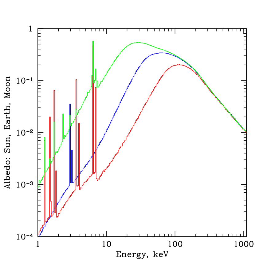
Figure 6: Albedo calculated for the CXB spectrum and different chemical compositions: solar photosphere (upper curve), Earth’s atmosphere (middle curve) and lunar surface (bottom curve).

The albedo is of course smallest in the Moon case, since heavier elements (compared to the Earth’s atmosphere or the solar photosphere) dominate the chemical composition. From this point of view the Moon is a better screen for the CXB than the Earth. For a typical satellite orbit (in particular for INTEGRAL), the angular size of the Moon is $\sim$30’ arcmin only (diameter) and obscuration by the Earth has a very strong advantage in terms of the subtended solid angle.

Both the Moon and the Sun could produce reflected signals associated with bright gamma-ray bursts or other transient events. For instance, recently the Helicon instrument on board the Coronas-F spacecraft detected a giant outburst from the soft gamma-ray repeater SGR 1806$-$20 reflected by the Moon (Mazets et al., 2005, Frederiks et al., 2007). In this particular observation the repeater and the Sun were both occulted by the Earth and only the emission reflected by the Moon was detected. If the mutual orientation of the objects had been different, the Sun could have produced a stronger (especially at energies below 100 keV) reflection signal.

6 Discussion

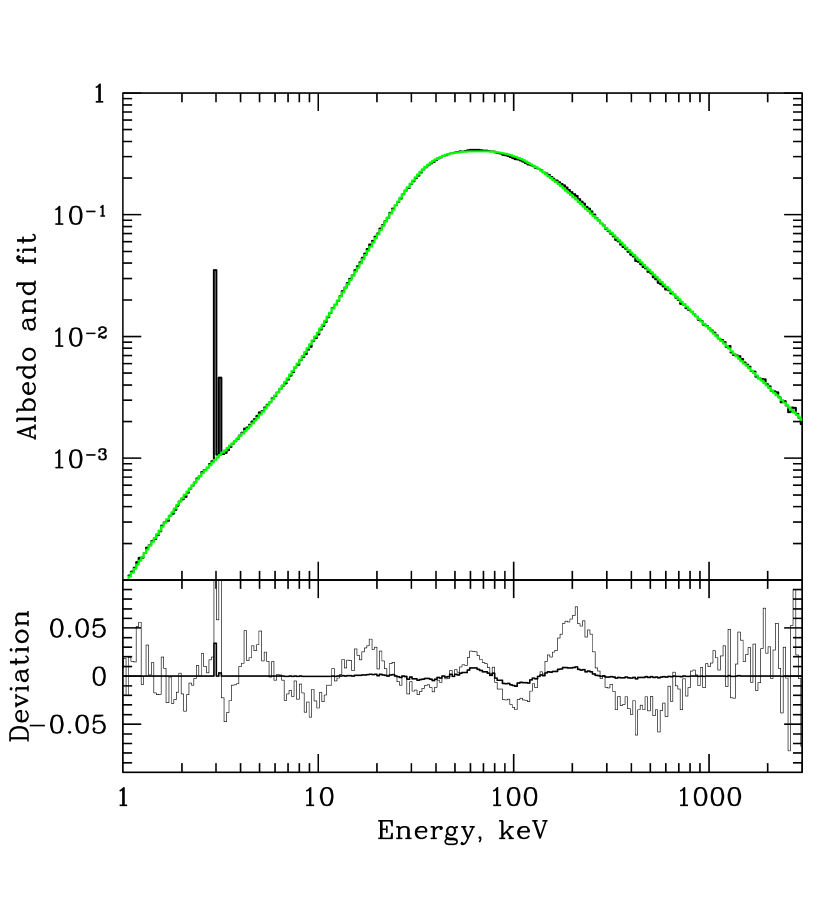
Figure 7: Comparison of the albedo $A(E)$ integrated over all angles (thick gray curve) and the analytic approximation (black curve). The thin curve in the lower panel shows the relative deviation of the simulated albedo from the analytic approximation. For the CXB studies more important is the absolute value of the difference between the simulated albedo and the analytic approximation. This difference is shown in the lower panel with the thick solid line. It is less than 1% at any energy in the 1-1000 keV range, except at the energy of the argon fluorescent line.

The energy dependence of the angle averaged Earth albedo (evaluated for the input spectrum given by equation (7)) can be approximated in the 1–1000 keV energy range by the following formula (see Fig.7):

$$A(E)=\frac{1.22}{\left(\frac{E}{28.5}\right)^{-2.54}+\left(\frac{E}{51.3}\right)^{1.57}-0.37}\times$$

$$\frac{2.93+\left(\frac{E}{3.08}\right)^{4}}{1+\left(\frac{E}{3.08}\right)^{4}}\times$$

$$\frac{0.123+\left(\frac{E}{91.83}\right)^{3.44}}{1+\left(\frac{E}{91.83}\right)^{3.44}}.$$ (14)

The factor $\Omega~{}(1-A(E))$ was used by Churazov et al. (2007) to relate the CXB spectrum and the decrease of hard X-ray flux observed by INTEGRAL during Earth observations. This factor provides a convenient way of correcting for the atmosphere reflection (for a given shape of the incident spectrum) as long as the full Earth disk is observed and the variations of the telescope response across the disk can be ignored (see section 4). In particular, it does not depend on the distance from the Earth. This universality breaks down if only part of the Earth disk is observed.

As is shown in Section 5.3, the angle averaged albedo exhibits a modest dependence on the assumed shape of the input spectrum. The uncertainty of 0.1 in the photon index of the input spectrum used for the albedo calculation translates into an error of $\sim$2.5% in the derived CXB flux at $\sim$50–100 keV. An additional uncertainty of $<$2% is associated with the slab approximation (see Section 5.2). As mentioned in Section 3, we did not model at all the polarization of the radiation. The incident isotropic radiation is unpolarized and the total flux reflected from the full Earth disk is of course also unpolarized. We also verified in explicit Monte-Carlo simulations that in calculating the spherical albedo, the substitution of the full Rayleigh scattering matrix by the Rayleigh phase function does not lead to albedo changes exceeding 1% for any value of the single scattering albedo $\lambda$.

At high energies (above $\sim$50–100 keV) the Earth’s atmosphere becomes a powerful source of hard radiation induced by the interaction of cosmic rays with the atmosphere. Typical spectra of the atmospheric emission are calculated in Sazonov et al. (2007). The reflection of the CXB photons in this regime is of secondary importance.

It is interesting to compare the reflected CXB emission from the Earth, Moon and Sun in the 1–1000 keV energy range to other components of their X-ray spectra (see e.g. Bhardwaj et al. 2007 for a review of X-ray properties of Solar system objects, especially in soft X-rays). Since we are concentrating on the energies above 1 keV, the main components are: i) direct or reflected solar radiation (dayside for planets), ii) reflected CXB emission and iii) emission induced by the interaction of cosmic rays with the atmospheres/surfaces of these objects . In Fig. 8 we show typical X-ray spectra (black solid lines) of the Sun during solar minimum, maximum and a flare, using the emission measures and gas temperatures from Peres et al. (2000). The dashed black line schematically shows the nonthermal emission component of a powerful solar flare, while the upper limits illustrate the constraints on the quiet Sun emission by RHESSI (Hannah et al. 2007). One can see that the reflected CXB emission (red solid line) is below the solar X-ray emission at energies below 5 keV even during the solar minimum. At higher energies the reflected component is more than two orders of magnitude fainter than the RHESSI upper limits, but potentially could be an important component in the Sun X-ray emission at these energies. The emission induced by cosmic-ray interactions with the solar atmosphere (Seckel et al. 1991, Sazonov et al. 2007) is shown by the magenta line. This component is weak compared to the reflected CXB radiation up to the highest energies of interest here (up to 1 MeV).

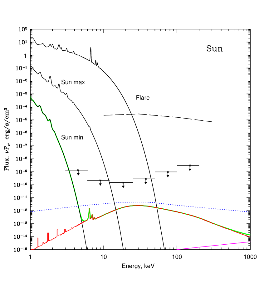
Figure 8: Reflected CXB emission (red line) from the Sun disk in comparison with other solar emission components. The three (soft) thermal spectra (solid black lines) are models of typical solar corona emission during solar minimum, maximum and flares (from Peres et al. 2000). The nonthermal component of a strong solar flare is shown with the dashed line. Upper limits show the constraints on the quiet Sun emission obtained by RHESSI (Hannah et al. 2007). The solid magenta line (bottom-right part of the plot) shows the emission induced by the interactions of cosmic rays with the solar atmosphere (Seckel et al. 1991, Sazonov et al. 2007). The thick solid green line shows the expected spectrum for the most quiet Sun. The CXB spectrum integrated over the solid angle subtended by the Sun disk is also shown for comparison (blue dotted line).

For the Moon (Fig. 9), the picture is quite different. The key feature is the presence of numerous fluorescent lines and small reflectivity in the continuum. In this figure we show the solar emission (again for solar minimum, maximum and a flare; black lines) reflected by the day-side of the Moon, along with the reflected CXB emission (red) and the cosmic-ray-induced component (magenta). The reflection of the solar radiation was observed from the lunar orbit with Luna 12 (Mandel’shtam et al., 1968), Apollo 15 and 16 (e.g. Adler et al., 1973) and more recently with SMART-1/D-CIXS (Grande et al. 2007). The black dotted line in Fig. 9 schematically shows the SMART-1/D-CIXS measurements, crudely converted to the units used in our plots from the published raw count spectra. The Moon albedo with respect to the CXB is smallest (compared to the Sun and the Earth), while the cosmic-ray induced emission is highest, since the Moon has no magnetic field, which for the Earth (and especially for the Sun) introduces a low-energy cutoff in the distribution of cosmic particles capable to reach the atmosphere/surface. The reflected CXB emission and the cosmic-ray induced component intersect near 40–50 keV. Below this energy (but above 1 keV) the dark side of the Moon is expected to be very X-ray dark (as indeed observed, Wargelin et al., 2004) – at the level of a few per cent of the CXB surface brightness, except for the fluorescent lines.

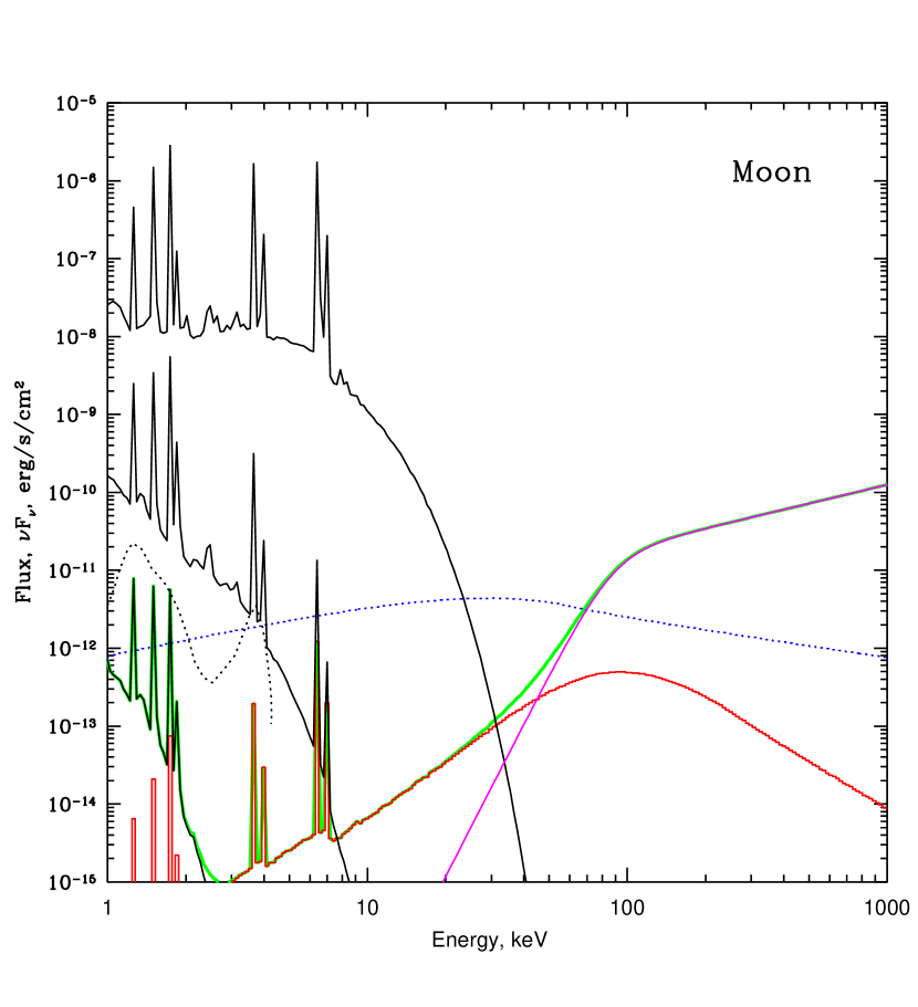
Figure 9: The same as in the previous figure, but for the Moon. The three spectra shown by black solid lines are the expected solar emission reflected from the dayside of the Moon for solar minimum, maximum and a flare (without the nonthermal component) respectively. The black dotted line schematically shows the recent SMART-1/D-CIXS measurements (Grande et al. 2007). The green thick solid line shows the total expected dayside emission from the Moon.

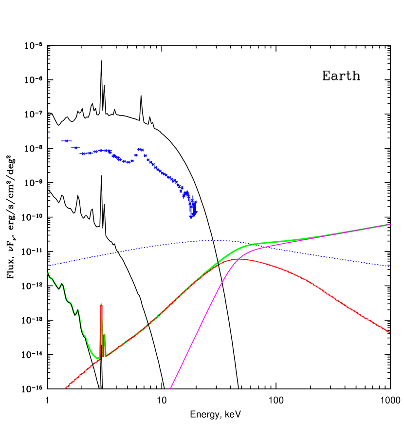
Figure 10: The same as in the previous figure, but for 1 square degree of the Earth’s atmosphere. Data points (blue asterisks) shows the reflected spectrum of the Earth dayside measured by RXTE during strong Solar flare (Molkov et al., private communications).

The Earth CXB albedo along with the reflected Solar radiation from the day-side, and cosmic ray induced component are shown in Fig.10. For comparison the reflected spectrum of the Earth day-side measured by RXTE during strong Solar flare (blue data points, Molkov et al., in preparation) is shown. The surface brightness of the X-ray aurora may have similar levels at energies below few tens of keV.

In terms of the albedo strength and the surface brightness of the cosmic ray induced emission the Earth case is intermediate between the Sun and the Moon cases (see also Fig.6). The “advantage” of the Earth is the large solid angle subtended by the Earth disk, which makes the signal larger for the wide-field instruments. The spectrum measured by INTEGRAL (Churazov et al., 2007) in the 5-200 keV range is a combination of the obscured CXB emission, reflected CXB emission and the atmospheric emission. The results were found to be consistent with expectations for the canonical CXB spectral shape and theoretical calculations of the albedo (this work) and the atmospheric emission (Sazonov et al., 2007). For INTEGRAL observations the albedo was making important correction in the energy range of 20-100 keV (see Fig. 10 in Churazov et al., 2007). At energies above 60-70 keV the signal measured by INTEGRAL was dominated by the cosmic ray induced component with the observed flux very close to the GEANT calculations by Sazonov et al., 2007. As pointed out in Churazov et al., 2007 and Sazonov et al., 2007 this overall agreement of the observed and predicted spectra strongly suggests that the Earth can be used as a useful calibrator for future hard X-ray and gamma-ray missions.

7 Conclusions

We calculated the Earth atmospheric albedo for the CXB radiation in the 1–1000 keV energy range. An analytic approximation for the angle averaged albedo is provided, which is especially useful when the whole Earth disk is observed. These calculations (along with the calculations of the cosmic ray induced atmospheric emission by Sazonov et al., 2007) were used in the analysis of the INTEGRAL observations of the Earth (Churazov et al., 2007) and a good agreement between predictions and measurements was found.

We further compared the Earth albedo to the CXB albedo for the Sun and the Moon and discuss other components contributing to the X-ray emission of these objects in the 1-1000 keV band.

The night-side of the Moon should be the X-ray darkest object in the solar system (subtending substantial solid angle for the telescope at the Earth orbit) in the energy range 1-30 keV, except at the energies of fluorescent lines of (e.g. Si or Fe).

The reflectivity of the Sun is on the contrary the highest and for exceptionally strong gamma-ray bursts or other transient events the signal reflected by the Sun below 100 keV (at the level of few $10^{-6}$ of the direct signal) will be stronger than by the Moon (see Mazets et al., 2005, Frederiks et al., 2007 for the discussion of a recent outburst from SGR1806-20 reflected by the Moon).

The Earth, because of the large solid angle subtended by its disk (for a wide-field telescope on the Earth orbit) is the most useful object for the CXB obscuration studies and potentially for the flux calibration of hard X-ray and gamma-ray missions at energies higher than 50-100 keV.

8 Acknowledgements

We are grateful to the referee, Juri Poutanen, for many useful comments and suggestions. This work was supported by the DFG grant CH389/3-2 and the program of the Russian Academy of Sciences ”Origin and evolution of stars and galaxies”.

References

- [\citeauthoryearAdler et al.1973] Adler I., et al., 1973, Moon, 7, 487
- [\citeauthoryearBasko, Sunyaev, & Titarchuk1974] Basko M. M., Sunyaev R. A., Titarchuk L. G., 1974, A&A, 31, 249
- [\citeauthoryearBiggs, Mendelsohn, & Mann1975] Biggs F., Mendelsohn L. B., Mann J. B., 1975, ADNDT, 16, 201
- [\citeauthoryearBhardwaj et al.2007] Bhardwaj A., et al., 2007, P&SS, 55, 1135
- [\citeauthoryearCravens et al.2006] Cravens T. E., Clark J., Bhardwaj A., Elsner R., Waite J. H., Maurellis A. N., Gladstone G. R., Branduardi-Raymont G., 2006, JGRA, 111, 7308
- [\citeauthoryearGeant4 Collaboration et al.2003] Agostinelli S., et al., 2003, NIMPA, 506, 250
- [\citeauthoryearGeorge & Fabian1991] George I. M., Fabian A. C., 1991, MNRAS, 249, 352
- [\citeauthoryearGhisellini, Haardt, & Matt1994] Ghisellini G., Haardt F., Matt G., 1994, MNRAS, 267, 743
- [\citeauthoryearGrande et al.2007] Grande M., et al., 2007, P&SS, 55, 494
- [\citeauthoryearChurazov et al.2007] Churazov E., et al., 2007, A&A, 467, 529
- [\citeauthoryearGruber et al.1999] Gruber D. E., Matteson J. L., Peterson L. E., Jung G. V., 1999, ApJ, 520, 124
- [\citeauthoryearCullen, Perkins, & Rathkopf1990] Cullen D. E., Perkins S. T., Rathkopf J. A. , ”The 1989 Livermore Evaluated Photon Data Library (EPDL),” UCRL-ID-103424, Lawrence Livermore National Laboratory (1990).
- [\citeauthoryearFrederiks et al.2007] Frederiks D. D., Golenetskii S. V., Palshin V. D., Aptekar R. L., Ilyinskii V. N., Oleinik F. P., Mazets E. P., Cline T. L., 2007, AstL, 33, 1
- [\citeauthoryearHannah et al.2007] Hannah I. G., Hurford G. J., Hudson H. S., Lin R. P., van Bibber K., 2007, ApJ, 659, L77
- [\citeauthoryearKaastra & Mewe1993] Kaastra J. S., Mewe R., 1993, A&AS, 97, 443
- [\citeauthoryearKippen2004] Kippen R. M., 2004, NewAR, 48, 221
- [\citeauthoryearMagdziarz & Zdziarski1995] Magdziarz P., Zdziarski A. A., 1995, MNRAS, 273, 837
- [\citeauthoryearMandel’shtam et al.1968] Mandel’shtam S. L., Tindo I. P., Cheremukhin G. S., Sorokin L. S., Dmitriev A. B., 1968, CosRe, 6, 100
- [\citeauthoryearMazets et al.2005] Mazets E.P., et al., 2005, astro-ph/0502541
- [\citeauthoryearMihalas1978] Mihalas D., 1978, Stellar atmospheres, San Francisco, W. H. Freeman and Co.
- [\citeauthoryearPeres et al.2000] Peres G., Orlando S., Reale F., Rosner R., Hudson H., 2000, ApJ, 528, 537
- [\citeauthoryearPoutanen, Nagendra, & Svensson1996] Poutanen J., Nagendra K. N., Svensson R., 1996, MNRAS, 283, 892
- [\citeauthoryearPozdniakov, Sobol, & Sunyaev1983] Pozdniakov L. A., Sobol I. M., Sunyaev R. A., 1983, ASPRv, 2, 189
- [\citeauthoryearSazonov et al.2007] Sazonov S., Churazov E., Sunyaev R., Revnivtsev M., 2007, MNRAS, 377, 1726
- [\citeauthoryearSeckel, Stanev, & Gaisser1991] Seckel D., Stanev T., Gaisser T. K., 1991, ApJ, 382, 652
- [\citeauthoryearSunyaev & Churazov1996] Sunyaev R. A., Churazov E. M., 1996, AstL, 22, 648
- [\citeauthoryearSunyaev, Uskov, & Churazov1999] Sunyaev R. A., Uskov D. B., Churazov E. M., 1999, AstL, 25, 199
- [\citeauthoryearWargelin et al.2004] Wargelin B. J., Markevitch M., Juda M., Kharchenko V., Edgar R., Dalgarno A., 2004, ApJ, 607, 596
- [\citeauthoryearWhite, Lightman, & Zdiziarski1988] White T. R., Lightman A. P., Zdiziarski A. A., 1988, ApJ, 331, 939
- [\citeauthoryearWillis et al.2005] Willis D. R., et al., 2005, A&A, 439, 245
- [\citeauthoryearvan de Hulst1974] van de Hulst H. C., 1974, A&A, 35, 209
- [\citeauthoryearVerner et al.1996] Verner D. A., Ferland G. J., Korista K. T., Yakovlev D. G., 1996, ApJ, 465, 487
- [\citeauthoryearVerner & Yakovlev1995] Verner D. A., Yakovlev D. G., 1995, A&AS, 109, 125