The temperature and ionization structure of the emitting gas in Hii galaxies: Implications for the accuracy of abundance determinations.

Guillermo F. Hägele¹, Enrique Pérez-Montero¹, Ángeles I. Díaz¹, Elena Terlevich² and Roberto Terlevich²
¹ Departamento de Física Teórica, C-XI, Universidad Autónoma de Madrid, 28049 Madrid, Spain
² INAOE, Tonantzintla, Apdo. Postal 51, 72000 Puebla, México
PhD fellow of Ministerio de Educación y Ciencia, Spain; guille.hagele@uam.esResearch Affiliate at IoA

(Accepted Received ; in original form )

Abstract

We propose a methodology to perform a self-consistent analysis of the physical properties of the emitting gas of HII galaxies adequate to the data that can be obtained with the XXI century technology. This methodology requires the production and calibration of empirical relations between the different line temperatures that should superseed currently used ones based on very simple, and poorly tested, photo-ionization model sequences.

As a first step to reach these goals we have obtained simultaneous blue to far red longslit spectra with the William Herschel Telescope (WHT) of three compact Hii galaxies selected from the Sloan Digital Sky Survey (SDSS) Data Release 2 (DR2) spectral catalog using the INAOE Virtual Observatory superserver. Our spectra cover the range from 3200 to 10500 Å, including the Balmer jump, the [Oii] $\lambda\lambda$ 3727,29 Å lines, the [Siii] $\lambda\lambda$ 9069,9532 Å doublet as well as various weak auroral lines such as [Oiii] $\lambda$ 4363 Å and [Siii] $\lambda$ 6312 Å.

For the three objects we have measured at least four line temperatures: T([Oiii]), T([Siii]), T([Oii]) and T([Sii]) and the Balmer continuum temperature T(Bac). These measurements and a careful and realistic treatment of the observational errors yield total oxygen abundances with accuracies between 5 and 9%. These accuracies are expected to improve as better calibrations based on more precise measurements, both on electron temperatures and densities, are produced.

The ionization structure found for the observed objects from the O⁺/O²⁺ and S⁺/S²⁺ ratios points to high values of the ionizing radiation, as traced by the values of the “softness parameter” $\eta$ which is less than one for the three objects. The use of line temperatures derived from T([Oiii]) based on current photoionization models yield for the two highest excitation objects, much higher values of $\eta$ which would imply lower ionizing temperatures. This is however inconsistent with the ionization structure as probed by the measured emission line intensities.

Finally, we have measured the T(Bac) for the three observed objects and derived temperature fluctuations. Only for one of the objects, the temperature fluctuation is significant and could lead to higher oxygen abundances by about 0.20 dex.

keywords:

galaxies: fundamental parameters - galaxies: starburst - galaxies: abundances - galaxies: temperature – ISM: abundances – Hii regions: abundances

^†^†pagerange: LABEL:firstpage–LABEL:lastpage^†^†pubyear: 2005

1 Introduction

Hii galaxies are low mass irregular galaxies with, at least, a recent episode of violent star formation (Melnick, Terlevich & Eggleton, 1985; Melnick, Terlevich & Moles, 1985) concentrated in a few parsecs close to their cores. The ionizing fluxes originated by these young massive stars dominate the light of this subclass of Blue Compact Dwarf galaxies (BCDs) which show emission line spectra very similar to those of giant extragalactic Hii regions (GEHRs; Sargent & Searle, 1970; French, 1980). Therefore, by applying the same measurement techniques as for Hii regions, we can derive the temperatures, densities and chemical composition of the interstellar gas in this type of generally metal-deficient galaxies. In some cases, it is possible to detect in these objects, intermediate-to-old stellar populations which have a more uniform spatial distribution than the bright and young stellar populations associated with the ionizing clusters (Schulte-Ladbeck et al., 1998). This older population produces a characteristic spectrum with absorption features which mainly affect the hydrogen recombination emission lines (Díaz, 1988), that is the Balmer and Paschen series in the spectral range of interest. In some cases, the underlying stellar absorptions can severely affect the ratios of Hi line pairs and hence the determination of the reddening constant (C(H $\beta$ )). They must therefore be measured with special care (see discussion in §3).

A considerable number of the blue objects observed at intermediate redshifts seem to have properties (mass, R_e, velocity width of the emission lines) similar to local Hii galaxies (Koo et al., 1994, 1995; Guzmán et al., 1996; Guzmán et al., 1998). In particular, those with $\sigma$ $<$ 65 km s^-1 follow the same $\sigma-L_{B}\ {\rm and}\ L_{H\beta}$ relation as seen in Hii galaxies (Melnick et al., 2000; Mas-Hesse et al., 2003; Terlevich et al., 2003; Siegel et al., 2005). Similar conclusion is drawn from recent studies on Lyman Break galaxies that also suggest that strong narrow emission line galaxies might have been very common in the past (e.g. Pettini et al., 2000; Pettini et al., 2001; Ellison et al., 2001). To detect possible evolutionary effects like systematic differences in their chemical composition, accurate and reliable methods for abundance determination are needed.

This is usually done by combining photoionization model results and observed emission line intensity ratios. There are several major problems with this approach that limit the confidence of present results. Among them: the effect of temperature structure in multiple-zone models (Pérez-Montero & Díaz, 2003); the presence of temperature fluctuations across the nebula (Peimbert, 2003); collisional and density effects on ion temperatures (Luridiana et al. 1999, Pérez-Montero & Díaz 2003); the presence of neutral zones affecting the calculation of ionization correction factors (ICFs; Peimbert et al. 2002); the ionization structure not adequately reproduced by current models (Pérez-Montero & Díaz, 2003); ionization vs. matter bounded zones, affecting the low ionization lines formed in the outer parts of the ionized regions (Castellanos, Díaz & Terlevich, 2002). On the other hand, the understanding of the age and evolutionary state of Hii galaxies require the use of self-consistent models for the ionizing stars and the ionized gas. However, model computed evolutionary sequences show important differences with observations (Stasińska & Izotov, 2003), including: (a) Heii is too strong in a substantial number of objects as compared to model predictions; (b) [Oiii]/H $\beta$ vs. [Oii]/H $\beta$ and [Oiii]/H $\beta$ vs. [Oi]/H $\beta$ are not well reproduced by evolutionary model sequences in the sense that predicted collisionally excited lines are too weak compared to observations; (c) there is a large spread in the [Nii]/[Oii] values (more than an order of magnitude) for galaxies with the same value of ([Oii]+[Oiii])/H $\beta$ in the metallicity range from 8 to 8.4 (see e.g. Pérez-Montero & Díaz 2005).

Table 1: Journal of observations. Right ascension, declination and redshift were obtained from the SDSS.

Object ID	spSpec SDSS	RA	Dec	z	Exposure (s)
SDSS J002101.03+005248.1	spSpec-51900-0390-445	5.254297	0.880038	0.098	1 $\times$ 1200 + 2 $\times$ 2400
SDSS J003218.60+150014.2	spSpec-51817-0418-302	8.077479	15.003949	0.018	1 $\times$ 1200 + 2 $\times$ 2400
SDSS J162410.11-002202.5	spSpec-52000-0364-187	246.042122	-0.367378	0.031	1 $\times$ 1200 + 3 $\times$ 1800

Table 2: SDSS photometric magnitudes obtained using the DR4 explore tools.

Object ID	u	g	r	i	z
SDSS J002101.03+005248.1	17.56	17.35	17.51	16.98	17.45
SDSS J003218.60+150014.2	17.04	16.49	16.53	16.74	16.65
SDSS J162410.11-002202.5	17.07	16.46	16.91	16.80	16.74

Substantial progress toward solving the problems listed above has to come from the accurate measurement of weak emission lines which will allow to derive [Oii], [Sii] and [Siii] temperatures and densities allowing to constrain the ionization structure as well as Balmer and Paschen discontinuities which will provide crucial information about the actual values of temperature fluctuations. It is possible that these fluctuations produce the observed differences between the abundances relative to hydrogen derived from recombination lines (RLs) and collisionally excited lines (CELs) when a constant electron temperature is assumed (Peimbert, 1967; Peimbert & Costero, 1969; Peimbert, 1971). These discrepancies have been observed in a good sample of objects, such as galactic Hii regions (e.g. Esteban et al., 2004; García-Rojas et al., 2005, 2006, and references therein), Hii regions in the Magellanic Clouds (e.g. Peimbert et al., 2000; Peimbert, 2003; Tsamis et al., 2003, and references therein), extragalactic Hii regions (e.g. Peimbert & Peimbert, 2003; Peimbert et al., 2005; Guseva et al., 2006, and references therein) and planetary nebulae (e.g. Rubin et al., 2002; Wesson et al., 2005; Liu et al., 2006; Liu, 2006; Peimbert & Peimbert, 2006, and references therein). Likewise, there are relatively recent theoretical works that study the possible causes of these discrepancies in abundance determinations using photoionization models of different complexity (e.g. Stasińska, 2005; Jamet et al., 2005; Tsamis & Péquignot, 2005, and references therein).

Unfortunately most of the available starburst and Hii galaxy spectra have only a restricted wavelength range (usually from about 3600 to 7000 Å) and do not have the adequate S/N to accurately measure the intensities of the weak diagnostic emission lines. Even the Sloan Digital Sky Survey (SDSS) spectra (Stoughton et al. 2002) do not cover simultaneously the [Oii] $\lambda\lambda$ 3727,29 and the [Siii] $\lambda$ 9069 Å lines. We have therefore undertaken a project with the aim of obtaining a database of top quality line ratios for a sample that includes the best objects for the task. The data is collected using exclusively two arm spectrographs in order to guarantee both high quality spectrophotometry in the whole spectral range from 3500 to 10500 Å and good spectral and spatial resolution. In this way we will be in a position to vastly improve constraints on the photoionization models including the mapping of the ionization structure and the measurement of temperature fluctuations about which very little is known.

In this first work we present observations of three Hii galaxies selected from the SDSS. Details regarding the selection of the objects as well as the observations are given in Section 2. Section 3 presents the results including line measuring techniques. The methodology for the derivation of gaseous physical conditions and elemental abundances is presented in Sections 4 and 5 respectively. The discussion of our results, including a detailed comparison with the SDSS data is presented in Section 6. Finally, Section 7 summarizes the main conclusions of our work.

2 Observations and data reduction

2.1 Object selection

SDSS constitutes a great base for statistical studies of the properties of galaxies. At this moment, the Fourth Data Release¹¹1http://www.sdss.org/dr4/ (DR4), the last one up to now, contains five band photometric data for about 18 $\times$ 10⁷ objects and more than 6.7 $\times$ 10⁵ spectra of galaxies, quasars and stars (Adelman-McCarthy et al. 2006). The spectroscopic data have a resolution (R) of 1800-2100 covering a spectral range from 3800 to 9200 Å, with a single 3 arcsec diameter aperture. The SDSS data were reduced and flux-calibrated using automatic pipelines. However, when we selected our objects on July 2004, the DR2²²2http://www.sdss.org/dr2/ was just available. Both data releases, DR2 and DR4, contain the same type of objects observed in the same five photometric bands and using the same spectroscopic configuration. DR2 has photometric data for over 88 million unique objects and about 3.7 $\times$ 10⁵ spectra (Abazajian et al. 2004). All the objects belonging to one data release are also included in the next ones, but some objects could have been re-calibrated or re-observed somehow. Using the implementation of the SDSS database in the INAOE Virtual Observatory superserver³³3http://ov.inaoep.mx/, we have selected from the whole SDSS DR2 the brightest nearby narrow emission line galaxies with very strong lines. Our selection parameters were:

Equivalent width of H $\alpha\,>$ 50 Å,

1.2 $<$ $\sigma$ (H $\alpha$ ) $<$ 7 Å,

redshift , z $<$ 0.2 and

H $\alpha$ flux, F(H $\alpha$ ) $>$ 4 $\times$ 10^-14 erg cm^-2 s^-1 Å^-1.

This preliminary list was then processed using BPT (Baldwin, Phillips & Terlevich 1981) diagnostic diagrams to remove AGN-like objects.

The final list consists of about 200 bonafide bright Hii galaxies. They show spectral properties indicating a wide range of gaseous abundances and ages of the underlying stellar populations (López, 2005).

From this list, the final set was selected by further restricting the sample to the largest H $\alpha$ flux and highest S/N objects.

From the 10 brightest of the final set we selected three HII galaxies to be observed in our one single night observing run. This final selection was made based on the relative positions of the sources in the sky allowing to optimize the observing time. The journal of observations is given in table 1 and the photometric characteristics of the objects are listed in table 2. Subsequently we have used the explore tool⁴⁴4http://cas.sdss.org/astro/en/tools/explore/ implemented in the DR3⁵⁵5http://www.sdss.org/dr3/ (Abazajian et al. 2005), which was available at the time of analysis, to extract again the three object SDSS spectra for comparison purposes.

Table 3: WHT instrumental configuration

	Spectral range	Disp.	FWHM	Spatial res.
	(Å)	(Å px^-1)	(Å)	(″ px^-1)
blue	3200-5700	0.86	2.5	0.2
red	5500-10550	1.64	4.8	0.2

2.2 Observational details

The blue and red spectra were obtained simultaneously using the ISIS double beam spectrograph mounted on the 4.2m William Herschel Telescope (WHT) of the Isaac Newton Group (ING) at the Roque de los Muchachos Observatory, on the Spanish island of La Palma. They were acquired on July the 18th 2004 during one single night observing run and under photometric conditions. EEV12 and Marconi2 detectors were attached to the blue and red arms of the spectrograph, respectively. The R300B grating was used in the blue covering the wavelength range 3200-5700 Å (centered at $\lambda_{c}$ = 4450 Å), giving a spectral dispersion of 0.86 Å pixel^-1. On the red arm, the R158R grating was mounted providing a spectral range from 5500 to 10550 Å ( $\lambda_{c}$ = 8025 Å) and a spectral dispersion of 1.64 Å pixel^-1. In order to reduce the readout noise of our images we have taken the observations with the ‘SLOW’ CCD speed. The pixel size for this set-up configuration is 0.2 arcsec for both spectral ranges. The slit width was $\sim$ 0.5 arcsec, which, combined with the spectral dispersions, yielded spectral resolutions of about 2.5 and 4.8 Å FWHM in the blue and red arms respectively. All observations were made at paralactic angle to avoid effects of differential refraction in the UV. The instrumental configuration, summarized in table 3 was planned in order to cover the whole spectrum from 3200 to 10550 Å providing at the same time a moderate spectral resolution. This guarantees the simultaneous measurement of the Balmer discontinuity and the nebular lines of [Oii] $\lambda\lambda$ 3727,29 and [Siii] $\lambda\lambda$ 9069,9532 Å at both ends of the spectrum, in the very same region of the galaxy. A good signal-to-noise ratio was also required to allow the detection and measurement of weak lines such as [Oiii] $\lambda$ 4363, [Sii] $\lambda\lambda$ 4068, 6717 and 6731, and [Siii] $\lambda$ 6312.

Several bias and sky flat field frames were taken at the beginning and at the end of each night in both arms. In addition, two lamp flat fields and one calibration lamp exposure were performed at each telescope position. The calibration lamp used was CuNe+CuAr. The images were processed and analyzed with IRAF⁶⁶6IRAF: the Image Reduction and Analysis Facility is distributed by the National Optical Astronomy Observatories, which is operated by the Association of Universities for Research in Astronomy, In. (AURA) under cooperative agreement with the National Science Foundation (NSF). routines in the usual manner. The procedure includes the removal of cosmic rays, bias substraction, division by a normalized flat field and wavelength calibration. Typical wavelength fits were performed using 30-35 lines in the blue and 20-25 lines in the red and polynomials of second to third order. These fits have been done at 117 different locations along the slit in each arm (beam size of 10 pixels) obtaining rms residuals between $\sim$ 0.1 and $\sim$ 0.2 pix.

Refer to caption — Figure 1: WHT spectra of SDSS J002101.03+005248.1 in the rest frame for the two observed ranges.

In the last step, the spectra were corrected for atmospheric extinction and flux calibrated. For the blue spectra, four standard star observations were used, allowing a good spectrophotometric calibration with an estimated accuracy of about 5%. Unfortunately, only one standard star could be used for the calibration of the red spectra. Nevertheless, after flux calibration, in the overlapping region of the spectra taken with each arm, the agreement in the average continuum level was good.

3 Results

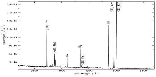
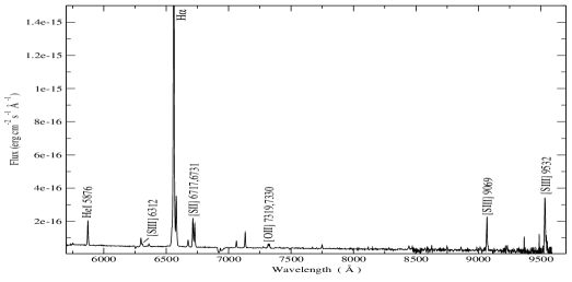
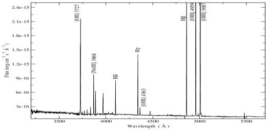
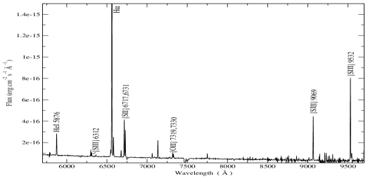
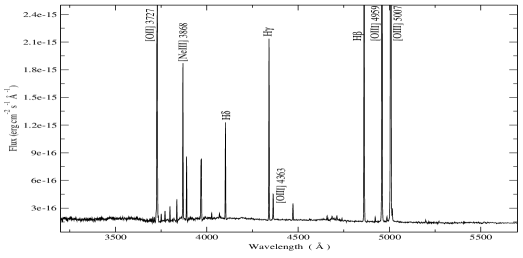
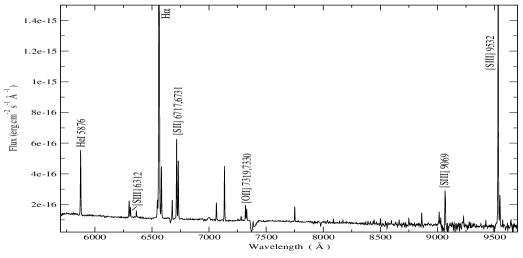
The WHT spectra of the observed galaxies with some of the relevant identified emission lines are shown in Figs. 1, 2 and 3. Each figure is split into two panels, showing the blue (upper panel) and red (lower panel) spectral ranges.

The emission line fluxes were measured using the SPLOT task of IRAF and are listed for the three observed galaxies in tables 4, 5, and 6. Column 1 of each table shows the wavelength and the name of the measured lines, as referred in García-Rojas et al. (2004). The observed emission line fluxes, $F(\lambda)$ (in units of H $\beta$ flux = 1000) with their corresponding errors, are presented in column 2. The measured equivalent widths (EW) are listed in column 3.

We have used two different ways to integrate the flux of a given line: (1) in the case of an isolated line or two blended and unresolved lines the intensity was calculated integrating between two points given by the position of the local continuum placed by eye; (2) if two lines are blended, but they can be resolved, we have used a multiple gaussian fit procedure to estimate individual fluxes. Following González-Delgado et al. (1994), Castellanos, Díaz & Terlevich (2002) and Pérez-Montero & Díaz (2003), the statistical errors associated with the observed emission fluxes have been calculated using the expression $\sigma_{l}$ = $\sigma_{c}$ N^1/2[1 + EW/(N $\Delta$ )]^1/2; where $\sigma_{l}$ is the error in the observed line flux, $\sigma_{c}$ represents the standard deviation in a box near the measured emission line and stands for the error in the continuum placement, N is the number of pixels used in the measurement of the line flux, EW is the line equivalent width, and $\Delta$ is the wavelength dispersion in angstroms per pixel. There are several lines affected by bad pixels, internal reflections or charge transfer in the CCD, telluric emission lines or atmospheric absorption lines. These cause the errors to increase, and, in some cases, they are impossible to quantify. In these cases we do not include these lines in the tables nore in our calculations. The only exception is the emission line [Siii] $\lambda$ 9069 for SDSS J162410.11-002202.5 which is affected by the strong narrow water-vapor lines present in the $\lambda$ 9300 - 9500 wavelength region (Díaz, Pagel & Wilson, 1985). We have listed the value of the measurement of this line in table 6, but all the physical parameters depending on its intensity were calculated using the theoretical ratio between this line and [Siii] $\lambda$ 9532, I(9069) $\approx$ 2.44 $\times$ I(9532) (Osterbrock, 1989). In some cases there is an observable line (e.g., [Cliii] $\lambda\lambda$ 5517,5537, several carbon recombination lines, Balmer or Paschen lines) for which it is impossible to give a precise measurement. This might be due to a low signal to noise between the line and the surrounding continuum. This is also the case for the Paschen jump that could not be measured even though it was observed, because it was very difficult to locate the continuum at both sides of the discontinuity with an acceptable accuracy.

The spectrum of SDSS J002101.03+005248.1 presents very wide lines (FWHM $\approx$ 7.5 Å for $\lambda$ $\approx$ 6600 Å) for the expected velocity dispersion in a low mass galaxy of this type. This could be due to an intrinsic velocity dispersion in this object, the interaction with another unobservable object or a projection effect on the line of sight. There are Hii galaxies that in fact are multiple systems, with two or more components, despite their “a priory” assumption of compactness (Zwicky, 1966; Sargent & Searle, 1970). In some cases, these systems show some evidence of interaction among their components (Telles, Melnick & Terlevich, 1997). For instance, IIZw40, which was first classified as a compact emission line galaxy by Sargent (1970), when observed with enough spatial resolution showed to be the merge of two separate subsystems (Baldwin, Spinrad & Terlevich, 1982). As a consequence, lines that should be resolved are blended in the spectrum of SDSS J002101.03+005248.1. Such is the case of H $\alpha$ and [Nii] $\lambda$ 6548 Å emission lines. We have resorted to the theoretical ratio, I(6584) $\approx$ 3 $\times$ I(6548), to decontaminate the observed flux of H $\alpha$ by the emission of [Nii] $\lambda$ 6548 and to derive the electron temperature of [Nii].

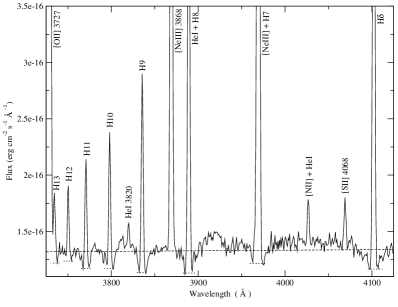
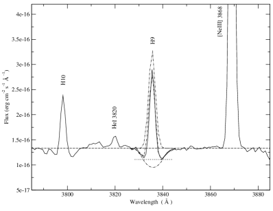
A conspicuous underlying stellar population is easily appreciable by the presence of absorption features that depress the Balmer and Paschen emission lines. The upper panel of Fig. 4 shows an example of this effect for the Balmer lines (H13 to H $\delta$ ) on an enlargement of the spectrum of SDSS J003218.60+150014.2, the object that presents the most relevant and appreciable absorption lines. The pseudo-continuum used to measure the line fluxes is also shown. We can clearly see the wings of the absorption lines implying that, even though we have used a pseudo-continuum, there is an absorbed fraction of the emitted flux that we are not able to measure with an acceptable accuracy (see discussion in Díaz 1988). This fraction is not the same for all lines, nore the ratios between the absorbed fractions and the emissions are the same. In order to quantify the effect of the underlying absorption on the measured emission line intensities, we have performed a multi-gaussian fit to the absorption and emission components seen in this galaxy. The fitting can be seen in the lower panel of Fig. 4. The difference between the measurements of the absorption subtracted lines and the ones obtained with the use of the pseudo-continuum is, for all Balmer lines, within the observational errors and, in fact, the additional fractional error introduced by the subtraction of the absorption component is almost inappreciable for the stronger lines. In the other two galaxies, the absorption wings in the Balmer lines are not prominent enough as to provide sensible results by the multi-gaussian component fitting. Therefore, we have doubled the error derived using the the expression for the statistical errors associated with the observed emission fluxes, ( $\sigma_{l}$ ).

The absorption features of the underlying stellar population may also affect the helium emission lines to some extent. However, these absorption lines are narrower than those of hydrogen (see, for example, González-Delgado et al., 2005), and therefore we cannot see their wings at both sides of the emission and we cannot define a pseudo-continuum to measure the line fluxes.

The reddening coefficient ( $C$ (H $\beta$ )) has been calculated assuming the galactic extinction law of Miller & Mathews (1972) with $R_{v}$ =3.2. $C(H\beta)$ was obtained in each case by performing a least square fit to the ratio between $F(\lambda)$ and $F(H\beta)$ to the theoretical values computed by Storey & Hummer (1995) using an iterative method to estimate $T_{e}$ and $n_{e}$ in each case. We have taken n_e equal to n([Sii]). Due to the large error introduced by the presence of the underlying stellar population (see discussion above) only the four strongest Balmer emission lines (H $\alpha$ , H $\beta$ , H $\gamma$ and H $\delta$ ) have been taken into account. The values obtained for $C(H\beta)$ and their corresponding errors, considered to be the uncertainties of the least square fittings, are listed in tables 4, 5, and 6 for each of the observed objects.

The emission line intensities corrected for reddening, relative to H $\beta$ ( $I(\lambda)$ ), and their corresponding errors are listed in column 4 of tables 4, 5, and 6. The errors were obtained propagating in quadratures the observational errors in the emission line fluxes and the reddening constant uncertainties. We have not taken into account errors in the theoretical intensities since they are much lower than the observational ones. Finally, the values listed in Column 5 of the tables indicate the fractional error in the line intensities calculated as explained above. These errors vary from a few percent for the more intense nebular emission lines (e.g. [Oiii] $\lambda\lambda$ 4959,5007, [Sii] $\lambda\lambda$ 6717,6731 or the strongest Balmer emission lines) to 10-16 % for the weakest lines that have less contrast with the continuum noise (e.g. Hei $\lambda\lambda$ 3820,7281, [Ariv] $\lambda$ 4740 or Oi $\lambda$ 8446). For the auroral lines, the fractional errors are between $\sim$ 3 and $\sim$ 9 %.

Table 4: Relative observed and reddening corrected line intensities [

F(H\beta)

I(H\beta)

=1000] for SDSS J002101.03+005248.1

	SDSS J002101.03+005248.1 - spSpec-51900-0390-445
$\lambda$ (Å)	WHT				SDSS
	$F(\lambda)$	-EW(Å)	$I(\lambda)$	Error (%)	$F(\lambda)$	-EW(Å)	$I(\lambda)$	Error (%)
3697 H17	4 $\pm$ 1	0.3	6 $\pm$ 1	11.7	—	—	—	—
3704 H16+Hei	11 $\pm$ 1	0.7	15 $\pm$ 1	9.9	—	—	—	—
3712 H15	8 $\pm$ 1	0.5	12 $\pm$ 2	15.5	—	—	—	—
3727 [Oii]^b	1190 $\pm$ 9	71.1	1634 $\pm$ 19	1.2	1598 $\pm$ 15	95.0	1789 $\pm$ 20	1.1
3750 H12	21 $\pm$ 2	1.3	29 $\pm$ 3	9.4	27 $\pm$ 3	1.8	30 $\pm$ 4	12.4
3770 H11	28 $\pm$ 2	1.7	38 $\pm$ 3	7.8	30 $\pm$ 3	2.0	33 $\pm$ 4	11.3
3798 H10	31 $\pm$ 2	2.0	42 $\pm$ 3	6.7	35 $\pm$ 3	2.3	39 $\pm$ 4	9.5
3835 H9	49 $\pm$ 5	3.2	65 $\pm$ 6	9.7	57 $\pm$ 6	4.0	63 $\pm$ 7	11.1
3868 [Neiii]	294 $\pm$ 6	17.7	388 $\pm$ 8	2.1	346 $\pm$ 6	21.6	382 $\pm$ 7	1.9
3889 Hei+H8	155 $\pm$ 9	9.7	203 $\pm$ 11	5.6	169 $\pm$ 9	11.2	186 $\pm$ 10	5.5
3968 [Neiii]+H7	226 $\pm$ 10	15.2	290 $\pm$ 13	4.4	248 $\pm$ 14	17.2	271 $\pm$ 15	5.5
4026 [Nii]+Hei	12 $\pm$ 1	0.8	15 $\pm$ 2	10.9	10 $\pm$ 1	0.6	10 $\pm$ 1	11.9
4068 [Sii]	11 $\pm$ 1	0.8	14 $\pm$ 1	8.6	12 $\pm$ 1	0.8	12 $\pm$ 1	9.7
4102 H $\delta$	213 $\pm$ 6	15.5	265 $\pm$ 7	2.8	230 $\pm$ 7	17.1	249 $\pm$ 8	3.2
4340 H $\gamma$	423 $\pm$ 7	33.6	499 $\pm$ 9	1.7	442 $\pm$ 9	36.5	469 $\pm$ 9	2.0
4363 [Oiii]	47 $\pm$ 2	3.8	56 $\pm$ 3	4.9	40 $\pm$ 2	3.3	42 $\pm$ 2	5.2
4471 Hei	37 $\pm$ 3	3.0	42 $\pm$ 3	7.9	36 $\pm$ 2	3.1	38 $\pm$ 3	6.9
4658 [Feiii]	10 $\pm$ 1	0.8	10 $\pm$ 1	7.1	11 $\pm$ 1	0.9	11 $\pm$ 1	12.3
4686 Heii	6 $\pm$ 1	0.5	7 $\pm$ 1	8.1	4 $\pm$ 1	0.3	4 $\pm$ 1	7.0
4713 [Ariv]+Hei	6 $\pm$ 1	0.6	7 $\pm$ 1	5.6	5 $\pm$ 1	0.5	5 $\pm$ 1	10.5
4740 [ArIV]	5 $\pm$ 1	0.4	5 $\pm$ 1	12.4	—	—	—	—
4861 H $\beta$	1000 $\pm$ 9	97.0	1000 $\pm$ 9	0.9	1000 $\pm$ 9	108.1	1000 $\pm$ 9	0.9
4881 [Feiii]	—	—	—	—	4 $\pm$ 1	0.4	4 $\pm$ 1	11.2
4921 Hei	6 $\pm$ 1	0.6	6 $\pm$ 1	8.6	8 $\pm$ 1	0.9	8 $\pm$ 1	6.9
4959 [Oiii]	1575 $\pm$ 13	151.5	1532 $\pm$ 13	0.8	1518 $\pm$ 10	160.0	1503 $\pm$ 10	0.6
4986 [Feiii]^c	9 $\pm$ 1	0.9	9 $\pm$ 1	10.2	10 $\pm$ 1	1.1	10 $\pm$ 1	10.5
5007 [Oiii]	4514 $\pm$ 26	439.4	4334 $\pm$ 26	0.6	4583 $\pm$ 26	489.4	4516 $\pm$ 26	0.6
5199 [Ni]	13 $\pm$ 1	1.5	12 $\pm$ 1	11.2	12 $\pm$ 1	1.4	11 $\pm$ 1	8.1
5270 [Feiii]^a	—	—	—	—	9 $\pm$ 1	1.1	9 $\pm$ 1	9.1
5755 [Nii]	7 $\pm$ 1	0.9	5 $\pm$ 1	7.1	7 $\pm$ 1	1.0	6 $\pm$ 1	6.9
5876 Hei	161 $\pm$ 8	22.3	127 $\pm$ 7	5.2	137 $\pm$ 7	22.0	125 $\pm$ 6	5.0
6300 [Oi]	54 $\pm$ 2	8.2	39 $\pm$ 1	3.3	47 $\pm$ 3	8.4	42 $\pm$ 3	6.1
6312 [Siii]	17 $\pm$ 1	2.6	12 $\pm$ 1	4.8	16 $\pm$ 1	2.8	14 $\pm$ 1	6.8
6364 [Oi]	15 $\pm$ 1	2.4	11 $\pm$ 1	5.2	14 $\pm$ 1	2.6	12 $\pm$ 1	6.8
6548 [Nii]	—	—	—	—	—	—	—	—
6563 H $\alpha$	4160 $\pm$ 39	658.3	2886 $\pm$ 40	1.4	3236 $\pm$ 8	607.1	2841 $\pm$ 22	0.8
6584 [Nii]	377 $\pm$ 12	59.6	260 $\pm$ 9	3.3	268 $\pm$ 6	50.8	235 $\pm$ 5	2.2
6678 Hei	47 $\pm$ 2	7.7	32 $\pm$ 1	4.6	38 $\pm$ 2	7.4	33 $\pm$ 2	6.0
6717 [Sii]	201 $\pm$ 7	33.8	136 $\pm$ 5	3.4	180 $\pm$ 5	35.4	157 $\pm$ 5	3.0
6731 [Sii]	159 $\pm$ 7	27.2	107 $\pm$ 5	4.3	136 $\pm$ 5	26.9	118 $\pm$ 4	3.6
7065 Hei	39 $\pm$ 2	7.2	25 $\pm$ 1	4.8	30 $\pm$ 2	6.5	25 $\pm$ 1	5.8
7136 [Ariii]	97 $\pm$ 4	18.5	62 $\pm$ 2	3.9	74 $\pm$ 3	17.5	63 $\pm$ 2	4.0
7155 [Feii]	—	—	—	—	3 $\pm$ 1	0.8	3 $\pm$ 1	12.5
7254 Oi	—	—	—	—	3 $\pm$ 1	0.8	3 $\pm$ 1	13.1
7281 Hei^a	10 $\pm$ 1	1.9	6 $\pm$ 1	7.0	8 $\pm$ 1	2.1	7 $\pm$ 1	5.6
7319 [Oii]^d	31 $\pm$ 1	6.2	20 $\pm$ 1	3.2	24 $\pm$ 1	5.8	21 $\pm$ 1	2.5
7330 [Oii]^e	21 $\pm$ 1	4.2	13 $\pm$ 1	4.5	18 $\pm$ 1	4.2	15 $\pm$ 1	3.6
7378 [Niii]	6 $\pm$ 1	1.2	4 $\pm$ 1	8.4	4 $\pm$ 1	0.9	3 $\pm$ 1	8.9
7412 [Niii]	7 $\pm$ 1	1.4	4 $\pm$ 1	7.9	—	—	—	—
7751 [Ariii]	23 $\pm$ 2	5.1	14 $\pm$ 1	6.9	22 $\pm$ 2	6.1	19 $\pm$ 1	7.4
8446 Oi	28 $\pm$ 2	7.2	16 $\pm$ 1	7.6	—	—	—	—
9069 [Siii]	230 $\pm$ 11	71.8	119 $\pm$ 6	5.0	—	—	—	—
9532 [Siii]	476 $\pm$ 16	504.4	239 $\pm$ 9	3.8	—	—	—	—
I(H $\beta$ )(erg seg^-1 cm^-2)	2.47 $\times$ 10^-14				3.38 $\times$ 10^-14
C(H $\beta$ )	0.51 $\pm$ 0.01				0.18 $\pm$ 0.01

^a possibly blend with an unknown line; ^b [Oii] $\lambda\lambda$ 3726 + 3729; ^c [Feiii] $\lambda\lambda$ 4986 + 4987; ^d [Oii] $\lambda\lambda$ 7318 + 7320; ^e [Oii] $\lambda\lambda$ 7330 + 7331.

Table 5: Relative observed and reddening corrected emission line intensities [

F(H\beta)

I(H\beta)

=1000] for SDSS J003218.60+150014.2.

	SDSS J003218.60+150014.2 - spSpec-51817-0418-302
$\lambda$ (Å)	WHT				SDSS
	$F(\lambda)$	-EW(Å)	$I(\lambda)$	Error (%)	$F(\lambda)$	-EW(Å)	$I(\lambda)$	Error (%)
3687 H19	10 $\pm$ 1	0.6	10 $\pm$ 1	8.5	—	—	—	—
3697 H17	13 $\pm$ 1	0.9	14 $\pm$ 1	8.6	—	—	—	—
3704 H16+Hei	19 $\pm$ 2	1.2	20 $\pm$ 2	8.4	—	—	—	—
3712 H15	15 $\pm$ 1	0.9	16 $\pm$ 1	7.5	—	—	—	—
3727 [Oii]^b	1466 $\pm$ 7	80.0	1573 $\pm$ 14	0.9	—	—	—	—
3734 H13	18 $\pm$ 1	1.2	20 $\pm$ 1	7.5	—	—	—	—
3750 H12	20 $\pm$ 2	1.3	21 $\pm$ 2	7.7	—	—	—	—
3770 H11	34 $\pm$ 2	2.3	37 $\pm$ 2	4.6	45 $\pm$ 3	3.0	51 $\pm$ 4	7.3
3798 H10	42 $\pm$ 2	2.8	45 $\pm$ 3	5.7	52 $\pm$ 4	3.6	59 $\pm$ 4	6.8
3820 Hei	7 $\pm$ 1	0.4	7 $\pm$ 1	14.3	—	—	—	—
3835 H9	61 $\pm$ 5	4.4	65 $\pm$ 5	8.3	59 $\pm$ 5	3.7	67 $\pm$ 5	7.7
3868 [Neiii]	350 $\pm$ 9	19.9	372 $\pm$ 10	2.6	370 $\pm$ 11	19.7	418 $\pm$ 12	2.9
3889 Hei+H8	184 $\pm$ 12	12.5	196 $\pm$ 12	6.3	181 $\pm$ 11	10.7	204 $\pm$ 13	6.2
3968 [Neiii]+H7	243 $\pm$ 12	17.0	257 $\pm$ 13	5.0	244 $\pm$ 15	17.4	272 $\pm$ 17	6.1
4026 [Nii]+Hei	14 $\pm$ 1	0.8	14 $\pm$ 1	7.1	15 $\pm$ 2	0.9	17 $\pm$ 2	12.1
4068 [Sii]	18 $\pm$ 1	1.1	19 $\pm$ 1	5.5	13 $\pm$ 1	0.8	15 $\pm$ 1	9.1
4102 H $\delta$	236 $\pm$ 9	17.2	247 $\pm$ 9	3.7	237 $\pm$ 8	17.5	261 $\pm$ 9	3.3
4340 H $\gamma$	482 $\pm$ 10	33.8	500 $\pm$ 10	2.0	440 $\pm$ 8	32.5	473 $\pm$ 9	1.9
4363 [Oiii]	60 $\pm$ 3	4.2	62 $\pm$ 3	4.8	60 $\pm$ 4	4.2	65 $\pm$ 4	6.4
4471 Hei	36 $\pm$ 2	2.7	37 $\pm$ 2	5.6	34 $\pm$ 3	2.4	36 $\pm$ 3	8.5
4658 [Feiii]	9 $\pm$ 1	0.7	9 $\pm$ 1	9.1	10 $\pm$ 1	0.7	10 $\pm$ 1	8.1
4686 Heii	13 $\pm$ 1	1.0	13 $\pm$ 1	6.3	14 $\pm$ 1	1.0	14 $\pm$ 1	8.6
4713 [Ariv]+Hei	11 $\pm$ 1	0.9	11 $\pm$ 1	5.5	11 $\pm$ 1	0.8	11 $\pm$ 1	11.4
4740 [Ariv]	5 $\pm$ 1	0.4	5 $\pm$ 1	12.9	3 $\pm$ 1	0.3	3 $\pm$ 1	11.9
4861 H $\beta$	1000 $\pm$ 8	89.6	1000 $\pm$ 8	0.8	1000 $\pm$ 9	86.7	1000 $\pm$ 9	0.9
4921 Hei	9 $\pm$ 1	0.8	9 $\pm$ 1	6.5	11 $\pm$ 1	0.9	11 $\pm$ 1	9.6
4959 [Oiii]	1592 $\pm$ 13	140.7	1582 $\pm$ 13	0.8	1651 $\pm$ 11	138.6	1631 $\pm$ 11	0.6
4986 [Feiii]^c	16 $\pm$ 1	1.4	15 $\pm$ 1	9.1	18 $\pm$ 2	1.5	18 $\pm$ 2	9.2
5007 [Oiii]	4649 $\pm$ 24	416.4	4607 $\pm$ 24	0.5	4863 $\pm$ 16	412.8	4778 $\pm$ 16	0.3
5015 Hei	23 $\pm$ 2	2.0	22 $\pm$ 2	8.8	24 $\pm$ 2	2.1	24 $\pm$ 2	7.8
5199 [Ni]	9 $\pm$ 1	0.9	9 $\pm$ 1	5.4	10 $\pm$ 1	0.9	9 $\pm$ 1	7.7
5270 [Feiii]^a	—	—	—	—	7 $\pm$ 1	0.7	7 $\pm$ 1	8.6
5755 [Nii]	—	—	—	—	—	—	—	—
5876 Hei	131 $\pm$ 6	16.0	124 $\pm$ 6	4.5	125 $\pm$ 6	15.0	113 $\pm$ 5	4.4
6300 [Oi]	30 $\pm$ 1	4.1	28 $\pm$ 1	3.9	30 $\pm$ 1	3.9	26 $\pm$ 1	2.5
6312 [Siii]	25 $\pm$ 1	3.3	23 $\pm$ 1	3.7	20 $\pm$ 1	2.6	17 $\pm$ 1	3.2
6364 [Oi]	11 $\pm$ 1	1.5	10 $\pm$ 1	5.9	10 $\pm$ 1	1.3	9 $\pm$ 1	3.0
6548 [Nii]	41 $\pm$ 3	5.8	37 $\pm$ 2	6.5	37 $\pm$ 2	5.2	31 $\pm$ 2	5.9
6563 H $\alpha$	3089 $\pm$ 19	435.5	2848 $\pm$ 30	1.0	3309 $\pm$ 16	462.8	2825 $\pm$ 27	0.9
6584 [Nii]	121 $\pm$ 5	17.3	112 $\pm$ 5	4.4	108 $\pm$ 3	15.1	92 $\pm$ 3	3.3
6678 Hei	35 $\pm$ 2	5.2	33 $\pm$ 2	5.4	34 $\pm$ 1	4.9	29 $\pm$ 1	2.4
6717 [Sii]	188 $\pm$ 5	30.3	173 $\pm$ 5	2.9	185 $\pm$ 4	26.9	156 $\pm$ 3	2.1
6731 [Sii]	136 $\pm$ 3	21.9	125 $\pm$ 3	2.5	135 $\pm$ 3	19.7	114 $\pm$ 2	2.1
7065 Hei	24 $\pm$ 2	4.2	22 $\pm$ 2	9.6	24 $\pm$ 2	3.9	20 $\pm$ 1	6.6
7136 [Ariii]	102 $\pm$ 3	17.7	92 $\pm$ 3	3.5	91 $\pm$ 4	15.0	75 $\pm$ 4	4.9
7155 [Feii]	5 $\pm$ 1	0.9	4 $\pm$ 1	13.6	—	—	—	—
7281 Hei^a	6 $\pm$ 1	1.1	6 $\pm$ 1	12.0	5 $\pm$ 1	0.9	4 $\pm$ 1	6.3
7319 [Oii]^d	27 $\pm$ 1	5.0	25 $\pm$ 1	4.0	24 $\pm$ 1	4.1	20 $\pm$ 1	2.9
7330 [Oii]^e	21 $\pm$ 1	3.9	19 $\pm$ 1	4.6	18 $\pm$ 1	3.1	15 $\pm$ 1	3.0
7751 [Ariii]	26 $\pm$ 3	5.1	23 $\pm$ 2	10.1	21 $\pm$ 1	3.9	17 $\pm$ 1	6.1
8446 Oi	7 $\pm$ 1	1.6	6 $\pm$ 1	15.7	6 $\pm$ 1	1.5	5 $\pm$ 1	11.0
8468 P17	3 $\pm$ 1	0.8	3 $\pm$ 1	12.5	—	—	—	—
8546 P15	—	—	—		7 $\pm$ 1	1.8	5 $\pm$ 1	10.8
8599 P14	14 $\pm$ 1	3.7	12 $\pm$ 1	10.7	10 $\pm$ 1	2.8	8 $\pm$ 1	8.6
8865 P11	17 $\pm$ 2	5.1	15 $\pm$ 2	11.2	16 $\pm$ 2	4.6	12 $\pm$ 1	9.4
9014 P10	25 $\pm$ 3	8.1	21 $\pm$ 2	10.7	—	—	—	—
9069 [Siii]	251 $\pm$ 10	76.4	217 $\pm$ 10	4.4	—	—	—	—
9532 [Siii]	518 $\pm$ 43	175.5	445 $\pm$ 38	8.5	—	—	—	—
9547 P8	75 $\pm$ 6	43.6	64 $\pm$ 5	8.5	—	—	—	—
I(H $\beta$ )(erg seg^-1 cm^-2)	1.23 $\times$ 10^-14				3.17 $\times$ 10^-14
C(H $\beta$ )	0.11 $\pm$ 0.01				0.22 $\pm$ 0.01

^a possibly blend with an unknown line; ^b [Oii] $\lambda\lambda$ 3726 + 3729; ^c [Feiii] $\lambda\lambda$ 4986 + 4987; ^d [Oii] $\lambda\lambda$ 7318 + 7320; ^e [Oii] $\lambda\lambda$ 7330 + 7331.

Table 6: Relative observed and reddening corrected emission line intensities [

F(H\beta)

I(H\beta)

=1000] for SDSS J162410.11-002202.5.

	SDSS J162410.11-002202.5 - spSpec-52000-0364-187
$\lambda$ (Å)	WHT				SDSS
	$F(\lambda)$	-EW(Å)	$I(\lambda)$	Error (%)	$F(\lambda)$	-EW(Å)	$I(\lambda)$	Error (%)
3687 H19	4 $\pm$ 1	0.3	5 $\pm$ 1	10.9	—	—	—	—
3692 H18	5 $\pm$ 1	0.4	6 $\pm$ 1	9.7	—	—	—	—
3697 H17	8 $\pm$ 1	0.8	11 $\pm$ 1	9.2	—	—	—	—
3704 H16+Hei	16 $\pm$ 1	1.5	22 $\pm$ 2	7.6	—	—	—	—
3712 H15	16 $\pm$ 1	1.5	22 $\pm$ 2	7.8	—	—	—	—
3727 [Oii]^b	1066 $\pm$ 13	91.0	1471 $\pm$ 22	1.5	1160 $\pm$ 13	96.81	1480 $\pm$ 19	1.3
3750 H12	20 $\pm$ 1	1.9	28 $\pm$ 2	6.7	18 $\pm$ 2	1.57	23 $\pm$ 2	9.3
3770 H11	24 $\pm$ 2	2.2	33 $\pm$ 2	6.7	24 $\pm$ 2	2.02	30 $\pm$ 3	8.3
3798 H10	35 $\pm$ 2	3.2	48 $\pm$ 3	6.7	36 $\pm$ 3	2.93	45 $\pm$ 4	8.4
3820 Hei	8 $\pm$ 1	0.7	11 $\pm$ 1	10.9	8 $\pm$ 1	0.61	10 $\pm$ 1	10.1
3835 H9	51 $\pm$ 4	4.6	69 $\pm$ 5	7.7	49 $\pm$ 3	4.17	61 $\pm$ 4	6.6
3868 [Neiii]	322 $\pm$ 8	25.8	428 $\pm$ 11	2.6	359 $\pm$ 8	27.28	444 $\pm$ 10	2.3
3889 Hei+H8	141 $\pm$ 9	12.8	186 $\pm$ 11	6.1	145 $\pm$ 9	12.61	178 $\pm$ 11	6.3
3968 [Neiii]+H7	249 $\pm$ 14	21.1	321 $\pm$ 18	5.7	238 $\pm$ 13	20.46	289 $\pm$ 15	5.3
4026 [Nii]+Hei	13 $\pm$ 1	1.0	16 $\pm$ 1	5.9	13 $\pm$ 1	1.11	16 $\pm$ 1	6.0
4068 [Sii]	12 $\pm$ 1	0.9	15 $\pm$ 1	8.2	11 $\pm$ 1	0.96	14 $\pm$ 1	10.8
4102 H $\delta$	207 $\pm$ 6	17.0	258 $\pm$ 8	3.0	212 $\pm$ 6	19.74	251 $\pm$ 7	2.9
4340 H $\gamma$	386 $\pm$ 7	34.6	457 $\pm$ 8	1.8	407 $\pm$ 6	39.78	463 $\pm$ 7	1.5
4363 [Oiii]	59 $\pm$ 2	5.0	70 $\pm$ 2	3.4	53 $\pm$ 1	5.02	60 $\pm$ 1	2.3
4471 Hei	37 $\pm$ 1	3.1	42 $\pm$ 2	3.8	35 $\pm$ 1	3.41	39 $\pm$ 1	3.2
4658 [Feiii]	9 $\pm$ 1	0.8	9 $\pm$ 1	8.2	10 $\pm$ 1	0.96	10 $\pm$ 1	10.0
4686 Heii	9 $\pm$ 1	0.8	10 $\pm$ 1	7.0	8 $\pm$ 1	0.75	8 $\pm$ 1	6.7
4713 [Ariv]+Hei	11 $\pm$ 1	2.0	11 $\pm$ 1	8.4	10 $\pm$ 1	1.01	10 $\pm$ 1	7.8
4740 [Ariv]	5 $\pm$ 1	0.4	5 $\pm$ 1	8.4	5 $\pm$ 1	0.48	5 $\pm$ 0	10.5
4861 H $\beta$	1000 $\pm$ 11	100.6	1000 $\pm$ 11	1.1	1000 $\pm$ 9	117.31	1000 $\pm$ 9	0.9
4881 [Feiii]	3 $\pm$ 1	0.3	3 $\pm$ 1	10.3	9 $\pm$ 1	0.31	9 $\pm$ 1	10.6
4921 Hei	10 $\pm$ 1	1.0	10 $\pm$ 1	4.3	8 $\pm$ 1	0.85	8 $\pm$ 1	8.7
4959 [Oiii]	1993 $\pm$ 14	191.7	1938 $\pm$ 14	0.7	2005 $\pm$ 12	220.10	1963 $\pm$ 12	0.6
4986 [Feiii]^c	13 $\pm$ 1	1.3	13 $\pm$ 1	6.6	11 $\pm$ 1	1.18	10 $\pm$ 1	6.3
5007 [Oiii]	5882 $\pm$ 28	565.3	5642 $\pm$ 28	0.5	6042 $\pm$ 18	659.56	5855 $\pm$ 18	0.3
5015 Hei	29 $\pm$ 3	2.8	28 $\pm$ 3	11.4	19 $\pm$ 2	2.07	18 $\pm$ 2	10.6
5159 [Feii]^a	4 $\pm$ 1	0.4	4 $\pm$ 1	12.6	—	—	—	—
5199 [Ni]	8 $\pm$ 1	0.9	7 $\pm$ 1	8.0	8 $\pm$ 1	0.85	7 $\pm$ 1	8.2
5270 [Feiii]^a	5 $\pm$ 1	0.6	5 $\pm$ 1	10.2	4 $\pm$ 1	0.47	4 $\pm$ 0	7.9
5755 [Nii]	3 $\pm$ 1	0.4	3 $\pm$ 1	8.4	—	—	—	—
5876 Hei	172 $\pm$ 4	20.4	135 $\pm$ 3	2.4	137 $\pm$ 3	21.54	113 $\pm$ 3	2.4
6300 [Oi]	42 $\pm$ 1	5.5	30 $\pm$ 1	2.2	36 $\pm$ 1	6.41	28 $\pm$ 1	2.2
6312 [Siii]	25 $\pm$ 1	3.3	18 $\pm$ 1	2.7	19 $\pm$ 1	3.31	15 $\pm$ 0	3.1
6364 [Oi]	15 $\pm$ 1	2.0	11 $\pm$ 1	3.0	13 $\pm$ 1	2.24	10 $\pm$ 0	3.3
6548 [Nii]	49 $\pm$ 2	6.8	34 $\pm$ 2	5.1	38 $\pm$ 2	6.82	28 $\pm$ 1	4.1
6563 H $\alpha$	4053 $\pm$ 33	566.3	2795 $\pm$ 36	1.3	3737 $\pm$ 17	680.37	2820 $\pm$ 24	0.9
6584 [Nii]	135 $\pm$ 3	18.8	93 $\pm$ 2	2.6	106 $\pm$ 2	19.27	80 $\pm$ 1	1.8
6678 Hei	51 $\pm$ 3	7.7	35 $\pm$ 2	5.9	45 $\pm$ 3	8.51	34 $\pm$ 2	5.9
6717 [Sii]	203 $\pm$ 5	29.2	136 $\pm$ 3	2.5	169 $\pm$ 3	32.21	125 $\pm$ 3	2.0
6731 [Sii]	147 $\pm$ 4	21.3	99 $\pm$ 3	2.7	123 $\pm$ 2	23.61	91 $\pm$ 2	2.1
7065 Hei	41 $\pm$ 3	6.2	26 $\pm$ 2	6.9	34 $\pm$ 2	7.25	25 $\pm$ 2	6.6
7136 [Ariii]	127 $\pm$ 4	20.5	80 $\pm$ 3	3.3	102 $\pm$ 3	22.14	72 $\pm$ 2	2.8
7254 Oi	2 $\pm$ 1	0.4	1 $\pm$ 1	9.2	—	—	—	—
7281 Hei^a	9 $\pm$ 1	1.5	6 $\pm$ 1	7.3	7 $\pm$ 1	1.62	5 $\pm$ 0	6.6
7319 [Oii]^d	35 $\pm$ 1	5.5	21 $\pm$ 1	3.1	29 $\pm$ 1	6.30	20 $\pm$ 1	2.5
7330 [Oii]^e	28 $\pm$ 1	4.5	18 $\pm$ 1	3.3	24 $\pm$ 1	5.16	16 $\pm$ 0	2.7
7751 [Ariii]	34 $\pm$ 2	5.8	20 $\pm$ 1	6.1	25 $\pm$ 1	5.81	16 $\pm$ 1	5.0
8392 P20	9 $\pm$ 1	2.0	5 $\pm$ 1	7.6	7 $\pm$ 1	2.16	4 $\pm$ 0	8.1
8413 P19	9 $\pm$ 1	2.1	5 $\pm$ 1	11.0	—	—	—	—
8438 P18	8 $\pm$ 1	1.7	4 $\pm$ 1	10.6	5 $\pm$ 1	1.67	3 $\pm$ 0	8.9
8446 Oi	11 $\pm$ 1	2.3	6 $\pm$ 1	7.7	10 $\pm$ 1	3.06	6 $\pm$ 0	4.9
8468 P17	8 $\pm$ 1	1.9	5 $\pm$ 1	9.7	6 $\pm$ 1	1.96	4 $\pm$ 0	9.1
8503 P16	20 $\pm$ 2	5.2	11 $\pm$ 1	10.8	—	—	—	—
8546 P15	13 $\pm$ 1	3.5	7 $\pm$ 1	11.1	9 $\pm$ 1	3.46	6 $\pm$ 1	9.2
8599 P14	12 $\pm$ 1	2.7	7 $\pm$ 1	9.3	13 $\pm$ 1	4.07	8 $\pm$ 1	9.1

Table 7: continued

Relative observed and reddening corrected emission line intensities [ $F(H\beta)$ = $I(H\beta)$ =1000] for SDSS J162410.11-002202.5.

	SDSS J002101.03+005248.1 - spSpec-51900-0390-445
$\lambda$ (Å)	WHT				SDSS
	$F(\lambda)$	-EW(Å)	$I(\lambda)$	Error (%)	$F(\lambda)$	-EW(Å)	$I(\lambda)$	Error (%)
8665 P13	15 $\pm$ 1	3.6	8 $\pm$ 1	8.3	16 $\pm$ 1	5.73	10 $\pm$ 1	7.5
8751 P12	23 $\pm$ 2	6.0	12 $\pm$ 1	9.2	18 $\pm$ 2	5.94	11 $\pm$ 1	8.7
8865 P11	33 $\pm$ 3	9.0	17 $\pm$ 2	10.4	24 $\pm$ 2	8.24	15 $\pm$ 1	10.1
9014 P10	34 $\pm$ 6	8.3	17 $\pm$ 3	17.6	—	—	—	—
9069 [Siii]^f	137 $\pm$ 9	66.8	70 $\pm$ 5	7.0	—	—	—	—
9532 [Siii]	809 $\pm$ 36	220.0	401 $\pm$ 19	4.8	—	—	—	—
9547 P8	91 $\pm$ 3	25.8	45 $\pm$ 2	4.1	—	—	—	—
I(H $\beta$ )(erg seg^-1 cm^-2)	5.03 $\times$ 10^-14				8.10 $\times$ 10^-14
C(H $\beta$ )	0.52 $\pm$ 0.01				0.39 $\pm$ 0.01

^a possibly blend with an unknown line; ^b [Oii] $\lambda\lambda$ 3726 + 3729; ^c [Feiii] $\lambda\lambda$ 4986 + 4987; ^d [Oii] $\lambda\lambda$ 7318 + 7320; ^e [Oii] $\lambda\lambda$ 7330 + 7331; ^f affected by atmospheric absorption bands.

4 Physical conditions of the gas

4.1 Electron densities and temperatures from forbidden lines

The physical conditions of the ionized gas, including electron temperatures and electron density, have been derived from the emission line data using the same procedures as in Pérez-Montero & Díaz (2003), based on the five-level statistical equilibrium atom approximation in the task TEMDEN, of the software package IRAF (De Robertis, Dufour & Hunt, 1987; Shaw & Dufour, 1995). The atomic coefficients used here are the same as in Pérez-Montero & Díaz (2003; see table 4 of that work), except in the case of O⁺ for which we have used the transition probabilities from Zeippen (1982) and the collision strengths from Pradham (1976), which offer more reliable nebular diagnostics results for this species (Wang et al., 2004). We have taken as sources of error the uncertainties associated with the measurement of the emission-line fluxes and the reddening correction and we have propagated them through our calculations. Electron densities have been derived from the [Sii] $\lambda\lambda$ 6717 / 6731 Å line ratio, which is representative of the low-excitation zone of the ionized gas. In all cases they were found to be lower than 200 particles per cubic centimeter, well below the critical density for collisional deexcitation. We have tried to derive the electron densities from the [Ariv] $\lambda\lambda$ 4713 / 4740 Å line ratio, by decontaminating the first one from the Hei contribution, but the derived density values had unacceptable errors due to their large and sensitive dependencies on the emission line intensities and the errors of the observed fluxes.

Several electron temperatures for each spectrum have been measured: T([Oii]), T([Oiii]), T([Sii]), T([Siii]) and T([Nii]). The [Nii] line at 5755 Å was not detected in the spectrum of SDSS J003218.60+150014.2 and therefore it was not possible to measure T([Nii]) for this object. Both the [Oii] $\lambda\lambda$ 7319,7330 Å and the [Nii] $\lambda$ 5755 Å lines can have a contribution by direct recombination which increases with temperature. Using the calculated [Oiii] electron temperatures, we have estimated these contributions to be less than 4% in all cases and therefore we have not corrected for this effect, although we have considered them when estimating the errors. The emission-line ratios used to calculate each temperature are summarized in table 8.

Table 8: Emission-line ratios used to derive electron densities and temperatures.

Diagnostic	Lines
n([Sii])	I(6717Å)/I(6731Å)
T([Oiii])	(I(4959Å)+I(5007Å))/I(4363Å)
T([Oii])	I(3727Å)/(I(7319Å)+I(7330Å))
T([Siii])	(I(9069Å)+I(9532Å))/I(6312Å)
T([Sii])	(I(6717Å)+I(6731Å))/(I(4068Å)+I(4074Å))
T([Nii])	(I(6548Å)+I(6584Å))/I(5755Å)

Table 9: Electron densities and temperatures for the observed galaxies using SDSS and WHT spectroscopy. Temperatures marked with asterisks have been deduced using equations from grids of photoionization models.

densities in $cm^{-3}$ and temperatures in 10⁴ $\degr$ K
	SDSS J002101.03+005248.1		SDSS J003218.60+150014.2		SDSS J162410.11-002202.5
	WHT	SDSS	WHT	SDSS	WHT	SDSS
n([Sii])	120 $\pm$ 68	77 $\pm$ 58	54:	56:	58:	66:
T([Oiii])	1.25 $\pm$ 0.02	1.13 $\pm$ 0.02	1.28 $\pm$ 0.02	1.28 $\pm$ 0.03	1.24 $\pm$ 0.01	1.16 $\pm$ 0.01
T([Oii])	1.03 $\pm$ 0.02	1.05 $\pm$ 0.02	1.35 $\pm$ 0.04	—	1.31 $\pm$ 0.03	1.23 $\pm$ 0.03
$\langle$ T([Oii]) $\rangle^{*}$	—	—	—	1.36	—	—
T([Siii])	1.31 $\pm$ 0.05	—	1.36 $\pm$ 0.07	—	1.26 $\pm$ 0.04	—
$\langle$ T([Siii]) $\rangle^{*}$	—	1.02	—	1.21	—	1.06
T([Sii])	0.86 $\pm$ 0.06	0.76 $\pm$ 0.06	1.03 $\pm$ 0.05	0.92 $\pm$ 0.06	1.04 $\pm$ 0.07	1.02 $\pm$ 0.09
T([Nii])	1.19 $\pm$ 0.05	1.36 $\pm$ 0.06	—	—	1.42 $\pm$ 0.08	—
$\langle$ T([Nii]) $\rangle^{*}$	—	—	1.35	1.36	—	1.23
T(Bac)	1.24 $\pm$ 0.27	—	0.96 $\pm$ 0.16	—	1.23 $\pm$ 0.22	—
T(H $\beta$ )	1.24 $\pm$ 0.31	—	1.02 $\pm$ 0.20	—	1.24 $\pm$ 0.26	—
T(Heii)	1.24 $\pm$ 0.29	—	0.98 $\pm$ 0.19	—	1.24 $\pm$ 0.23	—

The derived electron densities and temperatures for the three observed objects are listed in columns 2, 4 and 6 of table 9 along with their corresponding errors.

4.2 Balmer temperature

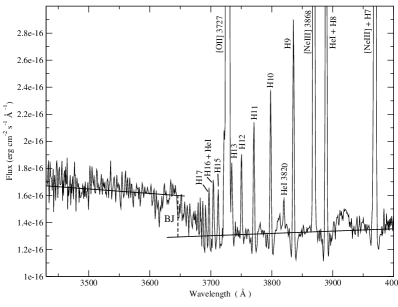
The Balmer temperature depends on the value of the Balmer jump (BJ) in emission. To measure this value we have adjusted the continuum at both sides of the discontinuity ( $\lambda_{B}$ = 3646 Å). Fig. 5 shows an example of the procedure for SDSS J003218.59+150014.2. The contribution of the underlying population (see Section 3) affect, among others, the hydrogen emission lines near the Balmer jump. The increase of the number of lines toward shorter wavelengths produces blends which tend to depress the continuum level to the right of the discontinuity and precludes the application of multi-gaussian component fittings. We have taken special care in the definition of this continuum by using a long baseline and spectral windows free of absorption lines. The uncertainties due to the presence of the underlying stellar population (different possible continuum placements) have been included in the errors of the measurements of the discontinuities. They are actually smaller than the error introduced by the fitting of stellar templates. Once the Balmer jump is measured, the Balmer continuum temperature (T(Bac)) is determined from the ratio of the Balmer jump flux to the flux of the H11 Balmer emission line using equation (3) in Liu et al. (2001):

T(Bac)\,=\,368\times(1\,+\,0.259y^{+}\,+\,3.409y^{2+})\Big{(}\frac{BJ}{H11}\Big{)}^{-3/2}\,K

where $y^{+}$ and $y^{2+}$ are the ionic abundances of singly and doubly ionized helium, He⁺/H⁺ and He²⁺/H⁺ (see §5), respectively, and BJ is in ergs cm^-2 s^-1 Å^-1. The derived values for T(Bac) are also listed in table 9.

5 Chemical abundances

Ionic and total abundances of He, O, S, N, Ne, Ar and Fe are obtained as detailed below and given in tables 10 and 11. We have derived the ionic chemical abundances of the different species using the stronger available emission lines detected in the analyzed spectra. The total abundances have been derived by taking into account, when required, the unseen ionization stages of each element, resorting to the most widely accepted ionization correction factors (ICF) for each species:

\frac{X}{H}=ICF(X^{+i})\cdot\frac{X^{+i}}{H^{+}}

5.1 Helium abundance

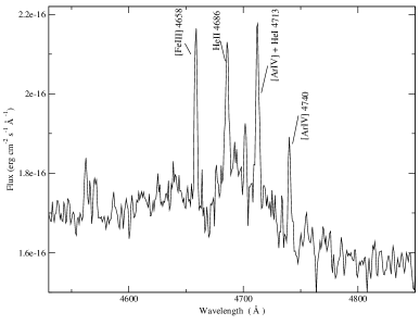
We have measured emission fluxes for 10 lines of Hei and 1 of Heii, although four of them are blended with another emission line and two are so weak that they cannot be used to derive the helium abundance with the necessary accuracy. We have therefore used the Hei $\lambda\lambda$ 4471, 5876, 6678 and 7065 Å, and Heii $\lambda$ 4686 Å lines to estimate the abundances of helium once and twice ionized respectively. These lines arise mainly from pure recombination, however they could have some contribution from collisional excitation as well as be affected by self-absorption and, if present, by underlying stellar absorption (see Olive & Skillman, 2001, 2004, for a complete treatment of these effects). We have taken the electron temperature of [Oiii] as representative of the zone where the He emission arises (i. e. T(Heii) $\simeq$ T([Oiii])) and we have used the equations given by Olive & Skillman to derive the He⁺/H⁺ value, using the theoretical emissivities scaled to H $\beta$ from Smits (1996) and the expressions for the collisional correction factors from Kingdon & Ferland (1995). We have not taken into account, however, the corrections for fluorescence (three of the used helium lines have a negligible dependence with optical depth effects and the observed objects have low densities) and the underlying stellar population. The three galaxies show in their spectra the signature of the presence of WR stars by the blue ‘bump’ around $\lambda$ 4600 Å therefore we have to take care when measuring the emission line flux of Heii $\lambda$ 4686 Å (see Fig. 6). We have used equation (9) from Kunth & Sargent (1983) to calculate the abundance of twice ionized helium. Then, for the total abundance we have directly added the two ionic abundances.

\frac{He}{H}\,=\,\frac{He^{+}+He^{2+}}{H^{+}}

The results obtained for each line and their corresponding errors are presented in table 10, along with the adopted value for He⁺/H⁺.

Table 10: Ionic and total chemical abundances for helium.

		SDSS J002101.03+005248.1		SDSS J003218.60+150014.2		SDSS J162410.11-002202.5
	$\lambda$ (Å)	WHT	SDSS	WHT	SDSS	WHT	SDSS
$He^{+}/H^{+}$	4471	0.086 $\pm$ 0.006	0.077 $\pm$ 0.006	0.076 $\pm$ 0.004	0.074 $\pm$ 0.006	0.086 $\pm$ 0.003	0.079 $\pm$ 0.002
	5876	0.096 $\pm$ 0.005	0.094 $\pm$ 0.006	0.096 $\pm$ 0.004	0.088 $\pm$ 0.003	0.104 $\pm$ 0.002	0.086 $\pm$ 0.002
	6678	0.087 $\pm$ 0.004	0.089 $\pm$ 0.006	0.089 $\pm$ 0.004	0.079 $\pm$ 0.001	0.094 $\pm$ 0.005	0.091 $\pm$ 0.005
	7065	0.094 $\pm$ 0.005	0.102 $\pm$ 0.006	0.086 $\pm$ 0.009	0.076 $\pm$ 0.006	0.104 $\pm$ 0.008	0.099 $\pm$ 0.007
	adopted	0.090 $\pm$ 0.005	0.090 $\pm$ 0.009	0.087 $\pm$ 0.007	0.080 $\pm$ 0.005	0.098 $\pm$ 0.007	0.085 $\pm$ 0.009
$He^{2+}/H^{+}$	4686	0.0006 $\pm$ 0.0001	0.0004 $\pm$ 0.0001	0.0011 $\pm$ 0.0001	0.0013 $\pm$ 0.0001	0.0008 $\pm$ 0.0001	0.0007 $\pm$ 0.0001
(He/H)		0.091 $\pm$ 0.005	0.090 $\pm$ 0.009	0.088 $\pm$ 0.007	0.081 $\pm$ 0.005	0.098 $\pm$ 0.007	0.085 $\pm$ 0.009

Table 11: Ionic and total chemical abundances, along with their corresponding ionization correction factors, derived from CELs. Logarithm of the S₂₃ parameter.

	SDSS J002101.03+005248.1		SDSS J003218.60+150014.2		SDSS J162410.11-002202.5
	WHT	SDSS	WHT	SDSS	WHT	SDSS
12+ $\log(O^{+}/H^{+})$	7.73 $\pm$ 0.06	7.73 $\pm$ 0.05	7.15 $\pm$ 0.06	7.10	7.18 $\pm$ 0.06	7.30 $\pm$ 0.05
12+ $\log(O^{2+}/H^{+})$	7.86 $\pm$ 0.02	8.01 $\pm$ 0.02	7.86 $\pm$ 0.02	7.87 $\pm$ 0.05	7.98 $\pm$ 0.02	8.08 $\pm$ 0.01
12+log(O/H)	8.10 $\pm$ 0.04	8.19 $\pm$ 0.03	7.93 $\pm$ 0.03	7.93	8.05 $\pm$ 0.02	8.14 $\pm$ 0.02
12+ $\log(S^{+}/H^{+})$	5.93 $\pm$ 0.11	6.13 $\pm$ 0.12	5.80 $\pm$ 0.06	5.88 $\pm$ 0.08	5.69 $\pm$ 0.08	5.67 $\pm$ 0.10
12+ $\log(S^{2+}/H^{+})$	5.91 $\pm$ 0.05	6.55	6.16 $\pm$ 0.06	6.34	6.14 $\pm$ 0.04	6.49
ICF( $S^{+}+S^{2+}$ )	1.12 $\pm$ 0.10	1.18	1.50 $\pm$ 0.15	1.57	1.61 $\pm$ 0.13	1.58
12+log(S/H)	6.27 $\pm$ 0.12	6.77	6.49 $\pm$ 0.11	6.67	6.48 $\pm$ 0.09	6.75
12+ $\log(N^{+}/H^{+})$	6.68 $\pm$ 0.04	6.62 $\pm$ 0.03	6.03	5.94	5.92 $\pm$ 0.06	5.98
log(N/O)	-1.06 $\pm$ 0.10	-1.12 $\pm$ 0.08	-1.11	-1.16	-1.26 $\pm$ 0.12	-1.32
12+ $\log(Ne^{2+}/H^{+})$	7.27 $\pm$ 0.03	7.42 $\pm$ 0.03	7.30 $\pm$ 0.06	7.27 $\pm$ 0.05	7.33 $\pm$ 0.03	7.44 $\pm$ 0.02
log(Ne/O)	-0.59 $\pm$ 0.06	-0.59 $\pm$ 0.06	-0.63 $\pm$ 0.06	-0.60 $\pm$ 0.07	-0.65 $\pm$ 0.05	-0.64 $\pm$ 0.03
12+ $\log(Ar^{2+}/H^{+})$	5.50 $\pm$ 0.05	5.67	5.65 $\pm$ 0.06	5.62	5.66 $\pm$ 0.04	5.70
12+ $\log(Ar^{3+}/H^{+})$	4.37 $\pm$ 0.05	—	4.32 $\pm$ 0.07	4.37 $\pm$ 0.05	4.36 $\pm$ 0.05	4.43 $\pm$ 0.05
ICF( $Ar^{2+}$ + $Ar^{3+}$ )	1.21 $\pm$ 0.06	—	1.01 $\pm$ 0.01	1.02	1.01 $\pm$ 0.01	1.02 $\pm$ 0.01
12+log(Ar/H)	5.59 $\pm$ 0.08	—	5.66 $\pm$ 0.06	5.63	5.66 $\pm$ 0.05	5.70
12+ $\log(Fe^{2+}/H^{+})$	5.50 $\pm$ 0.05	5.66 $\pm$ 0.07	5.42 $\pm$ 0.06	5.46 $\pm$ 0.06	5.48 $\pm$ 0.05	5.59 $\pm$ 0.05
ICF( $Fe^{2+}$ )	3.09 $\pm$ 0.33	3.52 $\pm$ 0.32	6.04 $\pm$ 0.84	6.63	7.00 $\pm$ 0.83	6.72 $\pm$ 0.63
12+log(Fe/H)	5.99 $\pm$ 0.10	6.20 $\pm$ 0.11	6.20 $\pm$ 0.12	6.28	6.32 $\pm$ 0.10	6.42 $\pm$ 0.09
log(S₂₃)	-0.22 $\pm$ 0.02	—	-0.02 $\pm$ 0.03	—	-0.10 $\pm$ 0.02	—

5.2 Ionic and total chemical abundances from forbidden lines

The oxygen ionic abundance ratios, O⁺/H⁺ and O²⁺/H⁺, have been derived from the [Oii] $\lambda\lambda$ 3727,29 Å and [Oiii] $\lambda\lambda$ 4959, 5007 Å lines respectively. The simultaneous determination of T([Oii]) and T([Oiii]) allows a more confident estimate of the total abundance of oxygen for which we have used the approximation:

\frac{O}{H}\,=\,\frac{O^{+}+O^{2+}}{H^{+}}

Regarding sulphur, we have derived S⁺ abundances using T([Sii]) values and the fluxes of the [Sii] emission lines at $\lambda\lambda$ 6717, 6731 Å. In the same way, the abundances of S²⁺ have been derived from the values of the directly measured T([Siii]) and the near-IR [Siii] $\lambda\lambda$ 9069, 9532 Å lines. The total sulphur abundance has been calculated using an ICF for S⁺+S²⁺ according to Barker’s (1980) formula, which is based on the photoionization models by Stasińska (1978):

ICF(S^{+}+S^{2+})=\left[1-\left(1-\frac{N(O^{+})}{N(O)}\right)^{\alpha}\right]^{-1/\alpha}

where $\alpha$ = 2.5 gives the best fit to the scarce observational data on S³⁺ abundances (Pérez-Montero et al. 2006).

The ionic abundance of nitrogen, N⁺/H⁺ has been derived from the intensities of the $\lambda\lambda$ 6548, 6584 Å lines and the measured electron temperature of [Nii] for objects SDSS J002101.03+005248.1 and SDSS J162410.11-002202.5. Then, the N/O abundance has been derived under the assumption that

\frac{N}{O}\,=\,\frac{N^{+}}{O^{+}}

In the case of SDSS J003218.60+150014.2, the [Nii] $\lambda$ 5755 Å line could not be measured and therefore we have assumed that T([Nii]) is equal to T([Oii]) and we have derived directly the N/O ratio according to the expression given in Pagel et al. (1992).

Neon is only visible in all the spectra via the [Neiii] emission line at $\lambda$ 3868 Å. For this ion we have taken the electron temperature of [Oiii], as representative of the high excitation zone. The total abundance of neon has been calculated assuming that:

\frac{Ne}{O}\,=\,\frac{Ne^{2+}}{O^{2+}}

Izotov et al. (2004) point out that this assumption can lead to an overestimate of Ne/H in objects with low excitation, where the charge transfer between O²⁺ and H⁰ becomes important. Nevertheless, in our case, it is probably justified given the high excitation of the observed objects.

The main ionization states of Ar in ionized regions are Ar²⁺ and Ar³⁺. The abundance of Ar²⁺ has been calculated by means of the emission line of [Ariii] $\lambda$ 7136 Å assuming that T([Ariii]) $\approx$ T([Siii]) (Garnett, 1992), while the ionic abundance of Ar³⁺ has been calculated under the assumption that T([Ariv]) $\approx$ T([Oiii]) and using the emission line of [Ariv] $\lambda$ 4740 Å. We could have used the blended emission line [Ariv]+HeI at $\lambda$ 4713 Å subtracting the helium contribution. However, due to the relative abundance of these species and the signal-to-noise ratio of this blended line, we prefer not to estimate this ionic abundance with such a large error. The total abundance of Ar has been calculated using the ICF(Ar²⁺+Ar³⁺) given by Izotov et al. (1994) which, in turn, has been derived from the photo-ionization models by Stasińska (1990) as:

	$\displaystyle ICF(Ar^{2+}+Ar^{3+})\,=\,\Big{[}0.99+0.091\Big{(}\frac{O^{+}}{O}\Big{)}{}$
			$\displaystyle{}-1.14\Big{(}\frac{O^{+}}{O}\Big{)}^{2}+0.077\Big{(}\frac{O^{+}}{O}\Big{)}^{3}\Big{]}^{-1}{}$

Finally, for iron we have used the emission line of [Feiii] $\lambda$ 4658 Å and the electron temperature of [Oiii]. We have taken the ICF(Fe²⁺) from Rodríguez & Rubin (2004), which yields:

ICF(Fe^{2+})\,=\,\Big{(}\frac{O^{+}}{O^{2+}}\Big{)}^{0.09}\cdot\Big{[}1+\frac{O^{2+}}{O^{+}}\Big{]}

The ionic and total abundances for each observed element are presented in columns 2, 4 and 6 of table 11, along with their corresponding errors.

6 Discussion

6.1 Comparison with SDSS data

In order to compare our results with those provided by SDSS spectra, we have measured the emission line intensities and equivalent widths on the SLOAN spectra of the three observed objects in the same way as described in Section 3. In order to allow an easy comparison between the results on both sets of spectra, we have listed these values in columns 6 to 9 of tables 4, 5, and 6.

Strong emission line fluxes relative to H $\beta$ measured on WHT and SDSS spectra differ by less than 10% for SDSS J003218.60+150014.2 and SDSS J162410.11-002202.5 and about 30% for SDSS J002101.03+005248.1. This is partially compensated by differences in the derived reddening constant so that reddening corrected emission line intensities relative to H $\beta$ differ by less that 10% for the [Oii] $\lambda\lambda$ 3727,29 Å line, about 15% for the weak [Oiii] $\lambda$ 4363 Å and [Siii] $\lambda$ 6312 Å lines and only a few percent for the strong [Oiii] $\lambda$ 5007 Å line. In fact, given the difference in aperture between both sets of observations, 0.5 and 3 arcsec for WHT and SDSS respectively, some differences are to be expected. While we have probably observed the bright cores of the galaxies where most of the light and present star formation is concentrated, the SDSS observations map a more extensive area which could include external diffuse zones. This is evidenced by the more conspicuous underlying stellar population detected in the WHT spectra which leads to lower values of the emission line equivalent widths. The best agreement between the two sets of measurements is found for SDSS J003218.60+150014.2, which is probably the more compact object, as evidenced by the difference in the measured H $\beta$ fluxes which is only a factor of 2 and the close agreement between the measured equivalent widths on the two spectra.

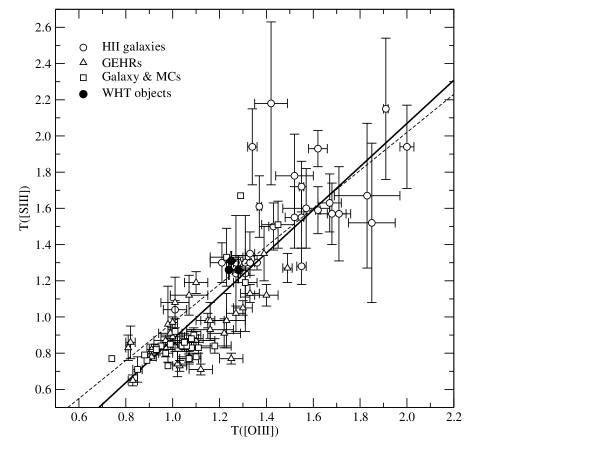
The SDSS spectra have been analyzed following the same methodology as explained in Sections 4 and 5 for the derivation of temperatures and abundances although, due to the different nature of the observations: different spectral coverage, signal-to-noise ratio and spectral resolution, some further assumptions had to be made. These refer mainly to the temperatures of the different ions. Regarding sulphur, the SDSS data do not reach the 9000-9600 Å range covered by the WHT spectra and therefore it was not possible to determine directly T([Siii]). The relation between T([Siii]) and T([Oiii]) is reproduced in Fig. 7. The sample used for comparison is a compilation of published data for which measurements of the nebular and auroral lines of [Oiii] and [Siii] exist, thus allowing the simultaneous determination of T([Oiii]) and T([Siii]). The sample is listed in Tables 1 and 2 of Pérez-Montero et al. (2006; objects not marked with a superscript b, as explained in the text), where the reader can find all the information concerning the data. The dashed line in the plot corresponds to the theoretical relation based on the grids of photoionization models described in Pérez-Montero & Díaz (2005),

T([S\textrm{\sc iii}])\,=\,1.05\,T([O\textrm{\sc iii}])\,-\,0.08

which differs slightly from the semi-empirical relation by Garnett (1992) mostly due to the introduction of the new atomic coefficients for S²⁺ from Tayal & Gupta (1999). The solid line in Fig. 7 corresponds to the actual fit to the data:

T([S\textrm{\sc iii}])=(1.19\pm 0.08)\,T([O\textrm{\sc iii}])-(0.32\pm 0.10)

The individual errors have not been taken into account in performing the fit. This fit is different from that found by Garnett (1992) that seems to reproduce well the M101 Hii region data analyzed by Kennicutt, Bresolin & Garnett (2003; KBG03). This is mostly due to the larger temperature baseline that we use. The object with the highest T([Siii]) in KBG03 is NGC5471A (12800 $\degr$ K); our sample includes high excitation Hii galaxies with T([Siii]) up to 24000 $\degr$ K, while including at the same time KBG03 sample. The introduction of the high excitation objects make the relation steeper and increases the error of the calibration. This illustrates the danger of extrapolating relations found for a restricted range of values. We have used our empirical calibration in order to obtain T([Siii]) for the SDSS spectra. The estimated errors introduced by the calibration are of the order of 12% for T([Siii]), i.e. between 1400 and 1500 $\degr$ K for the observed objects.

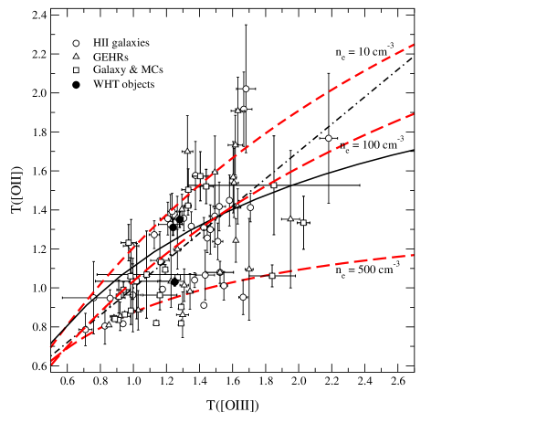
Likewise, the SDSS spectrum of J003218.60+150014.2 does not include the lines of [Oii] at $\lambda\lambda$ 3727,29 Å and therefore it was not possible to derive T([Oii]). Again, we have resorted to the model predicted relationship between T([Oii]) and T([Oiii]) found by Pérez-Montero & Díaz (2003) that takes explicitly into account the dependence of T([Oii]) on electron density. Three model sequences are represented in Fig. 8 correspondeing to three different values of the density: 10, 100 and 500 cm^-3 (dashed lines in the plot). The model sequence for n= 100 cm^-3 is very similar to the one derived from the models by Stasińska (1980). The sample used for comparison comprises the objects from Pérez-Montero & Díaz (2005) for which the derivation of T([Oii]) and T([Oiii]) has been possible. In this case, due to the dependence of T([Oii]) on electron density, there is not a single empirical calibration and it is not possible to give an estimate of the error introduced by the application of this procedure.

In the case of nitrogen, the [Nii] $\lambda$ 5755 Å line could be measured only in the SDSS spectrum of J002101.03+005248.1, due to poor signal to noise. In the other two cases, the assumption T([Nii]) = T([Oii]) has been made. This assumption is usually made in standard analysis techniques; however, there are not enough data for Hii galaxies to test it empirically.

Finally, the Balmer continuum temperature could not be calculated from the SDSS spectra due to lack of spectral coverage.

Concerning abundances, the S²⁺/H⁺ abundance ratios had to be calculated using the intensity of the weak auroral [Siii] line at $\lambda$ 6312 Å and, in the case of SDSS J003218.60+150014.2, the O⁺/H⁺ abundance ratio was derived using the [Oii] $\lambda\lambda$ 7319,7330 Å lines following the procedure described by Kniazev et al. (2004).

The values of electron density and temperatures, ionic and total abundances derived from the SDSS spectra are listed in columns 3, 5 and 7 of table 11, along with their corresponding errors in the cases where they have been derived from measured emission lines intensities. Otherwise, since the uncertainties introduced by the different assumptions made and the theoretical models used are impossible to quantify, no formal errors are given. These quantities should be considered as estimates and be used with caution.

For SDSS J003218.60+150014.2 the values we have obtained for densities, temperatures and abundances from the WHT and SDSS spectra are in excellent agreement within the observational errors, as expected from the close agreement between the measured emission line intensities. For the other two objects, the agreement can be considered as satisfactory, taking into account the difference in aperture between both sets of observations.

6.2 Gaseous physiscal conditions and element abundances

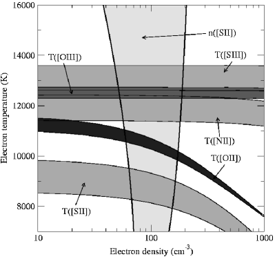
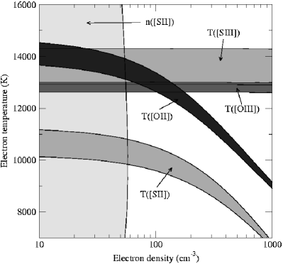
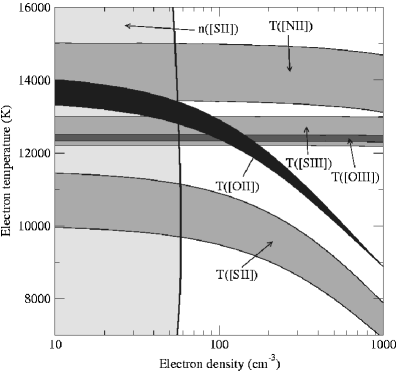
For the three observed objects we have been able to measure four electron temperatures: T([Oiii]), T([Oii]), T([Siii]) and T([Sii]). T([Nii]) has also been measured in two of the objects. The good quality of the data has allowed to reach accuracies of the order of 1% for T([Oiii]), 3% for T([Oii]) and 5% in the case of T([Nii]), T([Sii]) and T([Siii]). Figs. 9, 10 and 11 show the range of the measured line temperatures and electron density for objects SDSS J002101.03+005248.1, SDSS J003218.60+150014.2 and SDSS J162410.11-002202.5, respectively. The data for the latter two are very similar, although T([Nii]) could not be measured for SDSS J003218.60+150014.2. The width of the bands correspond to one $\sigma$ error. In the two cases T([Oiii]) and T([Siii]) overlap to some extent, while T([Oii]) is lower than T([Oiii]) in the first case and slightly higher than T([Oiii]) in the second.

The [Oii] and [Oiii] temperatures of the observed objects are shown in Fig. 8 together with the data of Hii galaxies, and galactic and extragalactic Hii regions from Pérez-Montero & Díaz (2005) and the photoionization models from Pérez-Montero & Díaz (2003) for electron densities n_e = 10, 100 and 500 cm^-3. The model sequences from Stasńska (1980; solid line) and Stasińska (1990; dashed-dotted line) are also plotted. This figure shows the effect of the electron density on the derived [Oii] temperature which decreases with increasing density. The data points populate the region of the diagram spanned by model sequences but the observational errors are too large to allow an adequate test of the photoionization models themselves. The temperatures derived for two of the observed objects: SDSS J003218.60+150014.2 and SDSS J162410.11-002202.5 lie close to the theoretical relation for an electron density of n_e= 10 cm ^-3, while for the other one: SDSS J002101.03+005248.1, they lie closer to sequences for electron densities larger than 100 cm^-3 . This is consistent with the trend shown by the values of n_e measured for the three objects.

For this last object, the value of T([Oii]) derived from the measured T([Oiii]) according to the widely used fit to the photoionization models by Stasińska (1990), is larger than the measured one by 2200 $\degr$ K which translates into a lower O⁺/H⁺ ionic ratio by a factor of 4 and a lower total oxygen abundance by 0.17 dex. It should be remarked that this is the procedure usually followed, even in the cases in which measured values of T([Oii]) exist (see Izotov, Thuan & Lipovetsky 1994). Also, in doing so, no uncertainties are attached to the T([Oii]) vs. T([Oiii]) relation with the final outcome of a reported T([Oii]) which carries only the usually small observational error found in the derivation of T([Oiii]) and translates into very small errors in the oxygen ionic and total abundances. Thus it is possible, and even frequent, to find reported values of T([Oii]) and T([Siii]) with quoted fractional errors lower than 1% and absolute errors actually less than that quoted for T([Oiii]) (Izotov & Thuan, 1998), and ionic O⁺/H⁺ ratios with errors of only 0.02 dex.

Recently, this procedure has been justified by Izotov et al. (2006) on the basis of an analysis of SDSS data. In this work it is argued that, despite a large scatter, the relation between T([Oii]) and T([Oiii]) derived from observations follows generally the one obtained by models, and therefore they adopt T([Oii]) as derived from their photoionization models. However, the large errors attached to the electron temperature determinations, in many cases around $\pm$ 2000 $\degr$ K for T([Oii]), actually precludes the test of such a statement. In fact, most of the data with the smallest error bars lie below and above the theoretical relation.

Regarding the [Siii] temperatures, our values fit well the relation between T([Oiii]) and T([Siii]) found by Garnett (1992) as can be seen in Fig. 7. For the objects for which we have measured T([Nii]), this is equal to T([Siii]) within the errors.

The abundances derived for the observed objects show the characteristic low values found in strong line Hii galaxies (Terlevich et al., 1991; Hoyos & Díaz, 2006): 12+log(O/H) = 8.0, within the errors, for SDSS J002101.03+005248.1 and SDSS J003218.60+150014.2 and slightly lower 12+log(O/H) = 7.9 for SDSS J162410.11-002202.5. The three objects have previous oxygen abundance determinations. They are part of the first edition of the SDSS Hii galaxies with oxygen abundance catalog, presented by Kniazev et al. (2004). These authors derived total oxygen abundances of 12+log(O/H) = 8.18 $\pm$ 0.04 for SDSS J002101.03+005248.1, 12+log(O/H) = 8.07 $\pm$ 0.02 for SDSS J003218.60+150014.2 and 12+log(O/H = 8.17 $\pm$ 0.01 for SDSS J162410.11-002202.5, higher than ours by 0.17 dex, but consistent with the values we obtain from the analysis of the SDSS spectra for two of the objects: SDSS J002101.03+005248.1 (12+log(O/H) = 8.19 $\pm$ 0.03) and SDSS J162410.11-002202.5 (12+log(O/H = 8.14 $\pm$ 0.02). For SDSS J003218.60+150014.2, our analysis of its SDSS spectrum yields a total oxygen abundance 12+log(O/H) = 7.93 $\pm$ 0.03, lower than theirs by 0.14 dex and closer to the value derived by Ugryumov et al. (2003) in their Hamburg/SAO Survey. The spectrum analyzed by Kniazev et al. (2004) was extracted from the first SDSS data release. This might point to a difference in the calibration routines of SDSS spectra from one release to the other.

The logarithmic N/O ratios found for the two galaxies for which there are T([Oii]) and T([Nii]) determinations are -1.06 $\pm$ 0.10 and -1.26 $\pm$ 0.12. For the third object we estimate a log(N/O) ratio of -1.11. They point to a constant value within the errors. It is worth noting that an analysis of the data along the lines discussed above, i. e. T([Oii]) derivation from T([Oiii]) according to Stasińska (1990) models, would provide for one of the objects, SDSS J002101.03+005248.1, an N/O ratio larger by a factor of 3 (log N/O = -0.64). Therefore it is not unplausible that part of the scatter found in the N/O vs. O/H diagram may be due to the methodology employed in the derivation of the N/O ratios. This is an important effect that should be explored further.

Finally, the log(S/O) ratios found for the three objects are: -1.83 $\pm$ 0.16, -1.44 $\pm$ 0.14 and -1.57 $\pm$ 0.11, barely consistent with solar (S/O = -1.39) except for J002101.03+005248.1 which is lower by a factor of about 2.7. The analysis of the data according to the conventional lines described above would rise this S/O ratio somewhat, but still keeping it below the solar value.

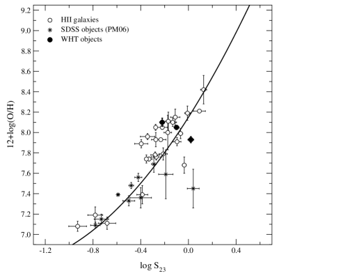
On the other hand, the measurement of the [Siii] IR lines allows the calculation of the sulphur abundance parameter S₂₃ (Vílchez & Esteban, 1996).

S_{23}\,=\,\frac{[S\textrm{\sc ii}]\,\lambda\lambda\,6717,31+[S\textrm{\sc iii}]\,\lambda\lambda\,9069,9532}{H\beta}

This parameter constitutes probably the best empirical abundance indicator for Hii galaxies, since contrary to what happens for the widely used O₂₃ (R₂₃) parameter (Pagel et al., 1979; Alloin et al., 1979), the calibration is linear up to solar abundances, thus solving the degeneration problem usually presented by this kind of objects. This is particularly dramatic for objects with log O₂₃ $\geq$ 0.8 and 12+log(O/H) $\geq$ 8.0 which can show the same value of the abundance parameter while having oxygen abundances that differ by up to an order of magnitude. About 40 % of the observed Hii galaxies belong to this category (see Díaz & Pérez-Montero, 1999). The logarithm of the S₂₃ parameter derived for our objects are given in the last row of table 11. Fig. 12 shows the points corresponding to the objects in the log S₂₃ vs. 12+log(O/H) diagram, together with their observational error, and labeled as WHT objects. The rest of the data correspond to Hii galaxies from Pérez-Montero & Díaz (2005) together with the data of ten SDSS BCD galaxies presented by Kniazev et al. (2004) and analyzed by Pérez-Montero et al. (2006) (these objects are labeled as SDSS objects). The solid line shows the calibration by Pérez-Montero & Díaz (2005). Three objects are seen to clearly deviate from this line. Two of them correspond to two of the galaxies of Kniazev et al. (2004) for which no data on the [Oii] 3727 line exist and therefore the O⁺/H⁺ ratio is derived from the red [Oii] 7325 lines. Both objects show low ionization parameters as estimated from the [Sii]/[Siii] ratio and relatively high values of O/H as derived from the [Nii]/H $\alpha$ calibration (Denicoló, Terlevich & Terlevich, 2002). The third object is Mrk709, an object that shows similar characteristics (see Pérez-Montero & Díaz 2003). These objects might be affected by shocks and deserve further study. Actually the accuracy of the S₂₃ calibration for Hii galaxies, as a family, is only 0.10 dex (see Pérez-Montero & Díaz 2005). But obviously, more observations are needed in order to improve the S₂₃ calibration and truly understand the origin of the observed dispersion.

6.3 Ionization structure

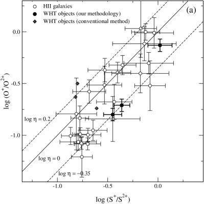
The ionization structure of a nebula depends essentially on the shape of the ionizing continuum and the nebular geometry and can be traced by the ratio of successive stages of ionization of the different elements. With our data it is possible to use the O⁺/O²⁺ and the S⁺/S²⁺ to probe the nebular ionization structure. In fact, Vílchez & Pagel (1988) showed that the quotient of these two quantities that they called “softness parameter” and denoted by $\eta$ is intrinsically related to the shape of the ionizing continuum and depends on geometry only slightly. If the simplifying assumption of spherical geometry and constant filling factor is made, the geometrical effect can be represented by the ionization parameter which, in turn can be estimated from the [Oii]/[Oiii] ratio. Actually, the [Oii]/[Oiii] ratio depends on stellar effective temperature which, in turn, depends on metallicity, in the sense that for a given stellar mass, stars of higher metallicity have a lower effective temperature. Since the three observed objects have similar values of this quotient (between 0.2 and 0.3), and show oxygen abundances in a very narrow range, we can assume they also share a common value for their ionization parameter. Under these circumstances, the value of $\eta$ points to the temperature of the ionizing radiation.

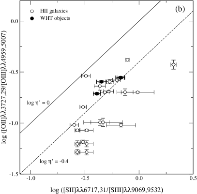
In panel (a) of Fig. 13 we show the relation between log(O⁺/O²⁺) and log(S⁺/S²⁺) for the observed objects (solid circles for values calculated using our methodology and solid diamonds for values derived using the conventional method) and the Hii galaxies from Pérez-Montero & Díaz (2005) for which the different oxygen and sulphur ionic ratios can be derived (open circles). In this diagram, diagonal lines correspond to constant values of $\eta$ ; the solid line corresponds to log $\eta$ = 0.00. The region above this line corresponds to $\eta$ $>$ 1 and the region below the line corresponds to $\eta$ $<$ 1. The dashed lines corresponds to log $\eta$ = -0.35 and log $\eta$ = 0.2 . As can be seen in the figure, Hii galaxies occupy the region of the diagram with -0.35 $\leq$ log $\eta$ $\leq$ 0.20, which corresponds to high values of the ionizing temperature according to Vílchez & Pagel (1988). Two of the observed objects lie on the log $\eta$ = -0.35 line. The third one, the one with the highest excitation, has log $\eta$ = -0.15. An analysis along the conventional lines commented in the previous subsection, would yield the same value of $\eta$ for the highest excitation object (although with different values of both O⁺/O²⁺ and S⁺/S²⁺ ratios) but widely different values of $\eta$ for the other two objects: 0.19 and 0.30 indicating much lower ionizing temperatures. This is inconsistent, however, with what is found if the same exercise is performed using the corresponding quotients of emission lines: log([Oii]/[Oiii]) vs log([Sii]/[Siii]), which does not require explicit knowledge of the line temperatures involved in the derivation of the ionic ratios, and therefore does not depend on the method to derive or estimate these temperatures. Panel (b) in Fig. 13 shows then the purely observational counterpart of panel (a). In this diagram diagonal lines represent constant values of log $\eta$ ’ defined by Vílchez & Pagel (1988) as:

	$\displaystyle log\,\eta{\textrm{'}}\,=\,log\Big{[}\frac{[O{\textrm{\sc ii}}]\lambda\lambda\,3727,29\,/\,[O{\textrm{\sc iii}}]\lambda\lambda\,4959,5007}{[S{\textrm{\sc ii}}]\lambda\lambda\,6717,31\,/\,[S{\textrm{\sc iii}}]\lambda\lambda\,9069,9532}\Big{]}{}$
			$\displaystyle{}\,=\,log\,\eta-\frac{0.14}{t_{e}}-0.16{}$

where t_e is the electron temperature in units of 10⁴. $\eta$ and $\eta$ ’ are related through the electron temperature but very weakly, so that a change in temperature from 7000 to 14000 $\degr$ K implies a change in log $\eta$ by 0.1 dex, inside observational errors. Also, log $\eta$ ’ is always less than log $\eta$ . In this diagram, the data for the three objects indicate values of log $\eta$ ’ between -0.39 and -0.25, consistent with what is found by our analysis but inconsistent with the results obtained following the conventional methodology. Metallicity calibrations based on abundances derived according to this conventional method are probably bound to provide metallicities which are systematically too high and should therefore be revised.

6.4 The temperature fluctuation scheme.

At the end of the 60s and beginning of the 70s, Peimbert (1967), Peimbert & Costero (1969), and Peimbert (1971) established a complete analytical formulation to study the discrepancies between the abundances relative to hydrogen derived from recombination lines (RLs) and from collisionally excited lines (CELs) when a constant electron temperature is assumed. In the first of these works, Peimbert proposed that this discrepancy is due to spatial temperature variations which can be characterized by two parameters: the average temperature weighted by the square of the density over the volume considered, T₀, and the root mean square temperature fluctuation, t². They are given by

\displaystyle T_{0}(X^{i+})\,=\,\frac{\int T_{e}\,N_{e}\,N(X^{i+})\,dV}{\int N_{e}\,N(X^{i+})\,dV}

(1)

and

\displaystyle t^{2}(X^{i+})\,=\,\frac{\int(T_{e}-T_{0}(X^{i+}))^{2}\,N_{e}\,N(X^{i+})\,dV}{T_{0}(X^{i+})^{2}\int N_{e}\,N(X^{i+})\,dV}

(2)

where N_e and N $(X^{+i}$ ) are the local electron and ion densities of the observed emission lines, respectively; T_e is the local electron temperature; and $V$ is the observed volume (Peimbert, 1967).

It is possible to obtain the values of T₀ and t² using different methods. One possibility is to compare the electron temperatures obtained using two independent ways. Generally, temperatures originated in different zones of the nebula are used, one that represents the warmest regions and another representative of the coldest ones. In the absence of temperatures derived from recombination lines, the temperatures estimated from the hydrogen discontinuities, either from Balmer or Paschen series, representative of the temperature of the neutral gas, can be used.

We have followed Peimbert et al. (2000); Peimbert et al. (2002, 2004) and Ruiz et al. (2003) to derive the values of T₀ and t² for our WHT spectra by combining the Balmer temperature, T(Bac), and the temperature derived from the collisional [Oiii] lines, T([Oiii]), therefore assuming a simple one-zone ionization scheme. Then, the relation for these two temperatures is given by:

\displaystyle T([O\textrm{\sc iii}])\,=\,T_{0}\,\Big{[}1+\frac{1}{2}\Big{(}\frac{91300}{T_{0}}-3\Big{)}\,t^{2}\Big{]}

(3)

and

\displaystyle T(Bac)\,=\,T_{0}\big{(}1-1.67t^{2}\big{)}

(4)

The solution of this system of equations for each galaxy along with their corresponding errors are listed in table 12. The temperature fluctuations are almost negligible for two of our objects. They have t²-values very similar to the ones derived by Luridiana et al. (2003) by combining observations from the literature and photoionization models for some BCDs and extragalactic Hii regions. Guseva et al. (2006) used the Balmer and Paschen jumps to determine the temperatures of the H⁺ zones of 22 low-metallicity Hii regions in 18 BCD galaxies, one extragalactic Hii region in M101 and 24 Hii emission-line galaxies selected from the DR3 of the SDSS. They found that these temperatures do not differ, in a statistical sense, from the temperatures of the [Oiii] zones, given t²-values are close to zero. The greater t²-value obtained for SDSS J003218.60+150014.2 is in the range of the values derived for giant extragalactic Hii regions (see González-Delgado et al., 1994; Peimbert et al., 2005; Jamet et al., 2005) or Hii regions in the Magellanic Clouds, such as 30 Doradus, LMC N11B and SMC N66 (Tsamis et al., 2003).

Table 12: T₀ and t² parameters

T₀ in 10⁴ $\degr$ K. Note that t² is always greater than zero.
name	T₀	t²
SDSS J002101.03+005248.1	1.24 $\pm$ 0.35	0.004 ${}^{+0.044}_{-0.004}$
SDSS J003218.60+150014.2	1.08 $\pm$ 0.21	0.066 $\pm$ 0.026
SDSS J162410.11-002202.5	1.24 $\pm$ 0.30	0.001 ${}^{+0.037}_{-0.001}$

In the limit of low densities and small optical depths, and for t² much lower than one, the electronic temperature for helium, T(Heii), is proportional to $\langle\alpha\rangle$ and $\beta$ , the average value of the power of the temperature for the helium lines used to calculate the ionic abundances of He⁺, and the corresponding one for H $\beta$ , respectively. Then, for $\langle\alpha\rangle$ different from $\beta$ , this temperature is given by equation (14) of Peimbert (1967):

\displaystyle T(He\textrm{\sc ii})\,=\,T(He\textrm{\sc ii},H\textrm{\sc ii})\,=\,T_{0}\Big{[}1+\big{(}\langle\alpha\rangle+\beta-1\big{)}\frac{t^{2}}{2}\Big{]}

(5)

The value of the power of the temperature for each helium line in the low density limit has been obtained from Benjamin et al. (1999). We have calculated $\langle\alpha\rangle$ as the average value of $\alpha$ weighted according to the observational errors (Peimbert et al., 2000). We have obtained values of $\langle\alpha\rangle$ equal to -1.37, -1.42, and -1.43 for SDSS J002101.03+005248.1, SDSS J003218.60+150014.2, and SDSS J162410.11-002202.5, respectively. The value of $\beta$ has been obtained from Storey & Hummer (1995) and is equal to -0.89. The results for T(Heii) and their corresponding errors are listed in the last row of table 9.

The temperature for H $\beta$ , T(H $\beta$ ), can be calculated from equation (20) in Peimbert & Costero (1969) as:

\displaystyle T(H\beta)=T_{0}\Big{[}1-0.95\,t^{2}\Big{]}

(6)

where we have taken $\beta$ = -0.89 as above. The derived values for T(H $\beta$ ) and their errors are also given in table 9.

The line temperature for a collisionally excited line, CEL, for t ${}^{2}\ll 1$ , ( $\Delta E_{CEL}$ /kT₀-1/2) $\neq$ 0, and $\alpha$ $\neq$ 0 is given by equation (20) of Peimbert & Costero (1969):

	$\displaystyle T_{CEL}\,=\,T_{0}\,\Big{\{}1{}$				(7)
			$\displaystyle{}+\Big{[}\frac{(\Delta E_{CEL}/kT_{0})^{2}-3\Delta E_{CEL}/kT_{0}+3/4}{\Delta E_{CEL}/kT_{0}-1/2}\Big{]}\frac{t^{2}}{2}\Big{\}}{}$		(7)

where $\Delta E_{CEL}$ = $\Delta E_{mn}$ is the energy difference, in eV, between the upper (m) and lower (n) levels respectively of the atomic transition that produces the line.

For the case of t ${}^{2}>$ 0, and assuming a one-zone ionization scheme, we can derive the ionic abundances using the values calculated for t² equal to zero, and equation (15) of Peimbert et al. (2004):

$\displaystyle\Big{[}\frac{N(X^{+i})}{N(H^{+})}\Big{]}_{t^{2}>0}\,=\,\frac{T(H\beta)^{-0.89}T(\lambda_{mn})^{0.5}}{T([O\textrm{\sc iii}])^{-0.37}}$		(8)
	$\displaystyle{}\times\,exp\Big{[}-\frac{\Delta E}{k\,T([O\textrm{\sc iii}])}+\frac{\Delta E}{k\,T(\lambda_{mn})}\Big{]}\,$
	$\displaystyle{}\times\,\Big{[}\frac{N(X^{+i})}{N(H^{+})}\Big{]}_{t^{2}=0}{}$

where T( $\lambda_{mn}$ ) is given by equation (7). Using this expression, we have calculated the effect of the temperature fluctuations on the O²⁺/H⁺ abundance. In fact, given the high excitation of the object, this ionic abundance carries the highest weight in the total abundance of oxygen. The recalculated value is 12+log(O²⁺/H⁺) = 8.09 $\pm$ 0.12 which yields a total oxygen abundance 12+log(O/H) = 8.12 $\pm$ 0.11. These values are higher than those given in Table 11 by 0.23 and 0.22 dex respectively.

7 Conclusions

We have performed a detailed analysis of newly obtained spectra of three Hii galaxies selected from the Sloan Digital Sky Survey Data Release 2, covering from 3200 to 10550 Å in wavelength. For the three objects we have measured four line temperatures: T([Oiii]), T([Siii]), T([Oii]) and T([Sii]) and the Balmer continuum temperature T(Bac). For two of the objects we have also measured T([Nii]). These measurements and a careful and realistic treatment of the observational errors yield total oxygen abundances with accuracies between 5 and 9%. The fractional error is as low as 2% for the ionic O²⁺/H⁺ ratio due to the small errors associated with the measurement of the strong nebular lines of [Oiii] and the derived T([Oiii]), but increases to 15% for the O⁺/H⁺ ratio. The accuracies are lower in the case of the abundances of sulphur (of the order of 20% for S⁺ and 12% for S²⁺) due to the presence of larger observational errors both in the measured line fluxes and the derived electron temperatures. The error increases further (up to 30%) for the total abundance of sulphur due to the uncertainties in the ICF.

This is in contrast with the small errors quoted for line temperatures other than T([Oiii]) in the literature, in part due to the commonly assumed methodology of deriving them from the measured T([Oiii]) through theoretical relations. These relations are found from photoionization models and no uncertainty is attached to them; therefore, the obtained line temperatures carries only the observational error found for the T([Oiii]) measurement. If this methodology were to be adopted, the theoretical relations should be adequately tested and empirical relations between the relevant line temperatures should be obtained in order to quantify the corresponding model uncertainties.

We have compared our obtained spectra with those downloaded from the SDSS DR3 finding a satisfactory agreement. The analysis of these spectra yields values of line temperatures and elemental ionic and total abundances which are in general agreement with those derived from the WHT spectra, although for most quantities, they can only be taken as estimates since, due to the lack of direct measurements of the required lines, theoretical models had to be used whose uncertainties are impossible to quantify. Unfortunately, the spectral coverage of SDSS precludes the simultaneous observation of the [Oii] $\lambda\lambda$ 3727,29 Å and [Siii] $\lambda\lambda$ 9069, 9532 Å lines, and therefore the analysis can never be complete.

The ionization structure found for the observed objects from the O⁺/O²⁺ and S⁺/S²⁺ ratios points to high values of the ionizing radiation as traced by the values of the “softness parameter” $\eta$ which is less than one for the three objects. Line temperatures derived from T([Oiii]) with the use of current photoionization models yield for the two highest excitation objects, much higher values of $\eta$ which would imply lower ionizing temperatures. This is however inconsistent with the ionization structure as probed by the measured emission line intensities.

Finally, we have measured the Balmer continuum temperature for the three observed objects and derived the temperature fluctuations as defined by Peimbert (1967). Only for one of the objects, the temperature fluctuation is significant and could lead to higher oxygen abundances by about 0.20 dex.

Acknowledgements

We are grateful to Jorge García-Rojas and César Esteban for calculating the effects of the temperature fluctuations over the derived ionic and total abundances. We are also grateful to an anonymous referee for his/her careful and constructive revision of the manuscript.

The WHT is operated in the island of La Palma by the Isaac Newton Group in the Spanish Observatorio del Roque de los Muchachos of the Instituto de Astrofísica de Canarias. We thank the Spanish allocation committee (CAT) for awarding observing time.

Funding for the creation and distribution of the SDSS Archive has been provided by the Alfred P. Sloan Foundation, the Participating Institutions, the National Aeronautics and Space Administration, the National Science Foundation, the US Department of Energy, the Japanese Monbukagakusho, and the Max Planck Society. The SDSS Web site is http://www.sdss.org.

The SDSS is managed by the ARC for the Participating Institutions. The Participating Institutions are the University of Chicago, Fermilab, the Institute for Advanced Study, the Japan Participation Group, The Johns Hopkins University, the Korean Scientist Group, Los Alamos National Laboratory, the Max Planck Institute for Astronomy (MPIA), the Max Planck Institute for Astrophysics (MPA), New Mexico State University, the University of Pittsburgh, the University of Portsmouth, Princeton University, the United States Naval Observatory, and the University of Washington.

This research has made use of the NASA/IPAC Extragalactic Database (NED) which is operated by the Jet Propulsion Laboratory, California Institute of Technology, under contract with the National Aeronautics and Space Administration.

This research has made use of the SIMBAD database, operated at CDS, Strasbourg, France.

This work has been partially supported by DGICYT project AYA-2004-02860-C03 and the Spanish MEC FPU grant AP2003-1821. Elena Terlevich acknowledges support from the Spanish MEC through a grant for a sabbatical visit SAB-2004-0148. She and Roberto would like to thank the hospitality of the Astrophysics Group of the UAM during the completion of this work.

References

Abazajian & et al. (2004) Abazajian K., et al. 2004, Astron. J., 128, 502
Abazajian & et al. (2005) Abazajian K., et al. 2005, Astron. J., 129, 1755
Adelman-McCarthy & et al. (2006) Adelman-McCarthy J. K., et al. 2006, Astrophys. J., Suppl. Ser., 162, 38
Alloin et al. (1979) Alloin D., Collin-Souffrin S., Joly M., Vigroux L., 1979, Astron. Astrophys., 78, 200
Baldwin et al. (1981) Baldwin J. A., Phillips M. M., Terlevich R., 1981, Publ. Astron. Soc. Pac., 93, 5
Baldwin et al. (1982) Baldwin J. A., Spinrad H., Terlevich R., 1982, Mon. Not. R. Astron. Soc., 198, 535
Barker (1980) Barker T., 1980, Astrophys. J., 240, 99
Benjamin et al. (1999) Benjamin R. A., Skillman E. D., Smits D. P., 1999, Astrophys. J., 514, 307
Castellanos et al. (2002) Castellanos M., Díaz A. I., Terlevich E., 2002, Mon. Not. R. Astron. Soc., 329, 315
de Robertis et al. (1987) de Robertis M. M., Dufour R. J., Hunt R. W., 1987, Royal Astronomical Society of Canada, Journal, 81, 195
Denicoló et al. (2002) Denicoló G., Terlevich R., Terlevich E., 2002, Mon. Not. R. Astron. Soc., 330, 69
Díaz (1988) Díaz A. I., 1988, Mon. Not. R. Astron. Soc., 231, 57
Díaz et al. (1985) Díaz A. I., Pagel B. E. J., Wilson I. R. G., 1985, Mon. Not. R. Astron. Soc., 212, 737
Díaz & Pérez-Montero (1999) Díaz A. I., Pérez-Montero E., 1999, in Walsh J. R., Rosa M. R., eds, Chemical Evolution from Zero to High Redshift Empirical Calibrations of Nebular Abundances: the Sulphur Abundance Parameter. pp 134–+
Ellison et al. (2001) Ellison S. L., Yan L., Hook I. M., Pettini M., Wall J. V., Shaver P., 2001, Astron. Astrophys., 379, 393
Esteban et al. (2004) Esteban C., Peimbert M., García-Rojas J., Ruiz M. T., Peimbert A., Rodríguez M., 2004, Mon. Not. R. Astron. Soc., 355, 229
French (1980) French H. B., 1980, Astrophys. J., 240, 41
García-Rojas et al. (2005) García-Rojas J., Esteban C., Peimbert A., Peimbert M., Rodríguez M., Ruiz M. T., 2005, Mon. Not. R. Astron. Soc., 362, 301
García-Rojas et al. (2006) García-Rojas J., Esteban C., Peimbert M., Costado M. T., Rodríguez M., Peimbert A., Ruiz M. T., 2006, Mon. Not. R. Astron. Soc., 368, 253
García-Rojas et al. (2004) García-Rojas J., Esteban C., Peimbert M., Rodríguez M., Ruiz M. T., Peimbert A., 2004, Astrophys. J., Suppl. Ser., 153, 501
Garnett (1992) Garnett D. R., 1992, Astron. J., 103, 1330
González-Delgado et al. (2005) González-Delgado R. M., Cerviño M., Martins L. P., Leitherer C., Hauschildt P. H., 2005, Mon. Not. R. Astron. Soc., 357, 945
González-Delgado et al. (1994) González-Delgado R. M., Pérez E., Tenorio-Tagle G., Vílchez J. M., Terlevich E., Terlevich R., Telles E., Rodríguez-Espinosa J. M., Mas-Hesse M., García-Vargas M. L., Díaz A. I., Cepa J., Castañeda H., 1994, Astrophys. J., 437, 239
Guseva et al. (2006) Guseva N. G., Izotov Y. I., Thuan T. X., 2006, astro-ph/0603134
Guzmán et al. (1998) Guzmán R., Jangren A., Koo D. C., Bershady M. A., Simard L., 1998, Astrophys. J. Letters, 495, L13+
Guzmán et al. (1996) Guzmán R., Koo D. C., Faber S. M., Illingworth G. D., Takamiya M., Kron R. G., Bershady M. A., 1996, Astrophys. J. Letters, 460, L5+
Hoyos & Díaz (2006) Hoyos C., Díaz A. I., 2006, Mon. Not. R. Astron. Soc., 365, 454
Izotov et al. (2004) Izotov Y. I., Stasińska G., Guseva N. G., Thuan T. X., 2004, Astron. Astrophys., 415, 87
Izotov et al. (2006) Izotov Y. I., Stasińska G., Meynet G., Guseva N. G., Thuan T. X., 2006, Astron. Astrophys., 448, 955
Izotov & Thuan (1998) Izotov Y. I., Thuan T. X., 1998, Astrophys. J., 500, 188
Izotov et al. (1994) Izotov Y. I., Thuan T. X., Lipovetsky V. A., 1994, Astrophys. J., 435, 647
Jamet et al. (2005) Jamet L., Stasińska G., Pérez E., González Delgado R. M., Vílchez J. M., 2005, Astron. Astrophys., 444, 723
Kennicutt et al. (2003) Kennicutt R. C., Bresolin F., Garnett D. R., 2003, Astrophys. J., 591, 801(KBG03)
Kingdon & Ferland (1995) Kingdon J., Ferland G. J., 1995, Astrophys. J., 442, 714
Kniazev et al. (2004) Kniazev A. Y., Pustilnik S. A., Grebel E. K., Lee H., Pramskij A. G., 2004, Astrophys. J., Suppl. Ser., 153, 429
Koo et al. (1994) Koo D. C., Bershady M. A., Wirth G. D., Stanford S. A., Majewski S. R., 1994, Astrophys. J. Letters, 427, L9
Koo et al. (1995) Koo D. C., Guzmán R., Faber S. M., Illingworth G. D., Bershady M. A., Kron R. G., Takamiya M., 1995, Astrophys. J. Letters, 440, L49
Kunth & Sargent (1983) Kunth D., Sargent W. L. W., 1983, Astrophys. J., 273, 81
Liu (2006) Liu X. ., 2006, astro-ph/0605082
Liu et al. (2006) Liu X.-W., Barlow M. J., Zhang Y., Bastin R. J., Storey P. J., 2006, Mon. Not. R. Astron. Soc., pp 404–+
Liu et al. (2001) Liu X.-W., Luo S.-G., Barlow M. J., Danziger I. J., Storey P. J., 2001, Mon. Not. R. Astron. Soc., 327, 141
López (2005) López J., 2005, MSc Thesis. INAOE
Luridiana et al. (2003) Luridiana V., Peimbert A., Peimbert M., Cerviño M., 2003, Astrophys. J., 592, 846
Luridiana et al. (1999) Luridiana V., Peimbert M., Leitherer C., 1999, Astrophys. J., 527, 110
Mas-Hesse et al. (2003) Mas-Hesse J. M., Kunth D., Tenorio-Tagle G., Leitherer C., Terlevich R. J., Terlevich E., 2003, Astrophys. J., 598, 858
Melnick et al. (1985) Melnick J., Terlevich R., Eggleton P. P., 1985, Mon. Not. R. Astron. Soc., 216, 255
Melnick et al. (1985) Melnick J., Terlevich R., Moles M., 1985, Revista Mexicana de Astronomia y Astrofisica, 11, 91
Melnick et al. (2000) Melnick J., Terlevich R., Terlevich E., 2000, Mon. Not. R. Astron. Soc., 311
Miller & Mathews (1972) Miller J. S., Mathews W. G., 1972, Astrophys. J., 172, 593
Olive & Skillman (2001) Olive K. A., Skillman E. D., 2001, New Astronomy, 6, 119
Olive & Skillman (2004) Olive K. A., Skillman E. D., 2004, Astrophys. J., 617, 29
Osterbrock (1989) Osterbrock D. E., 1989, Astrophysics of gaseous nebulae and active galactic nuclei. Mill Valley, CA, University Science Books
Pagel et al. (1979) Pagel B. E. J., Edmunds M. G., Blackwell D. E., Chun M. S., Smith G., 1979, Mon. Not. R. Astron. Soc., 189, 95
Pagel et al. (1992) Pagel B. E. J., Simonson E. A., Terlevich R. J., Edmunds M. G., 1992, Mon. Not. R. Astron. Soc., 255, 325
Peimbert (2003) Peimbert A., 2003, Astrophys. J., 584, 735
Peimbert et al. (2002) Peimbert A., Peimbert M., Luridiana V., 2002, Astrophys. J., 565, 668
Peimbert et al. (2005) Peimbert A., Peimbert M., Ruiz M. T., 2005, Astrophys. J., 634, 1056
Peimbert (1967) Peimbert M., 1967, Astrophys. J., 150, 825
Peimbert (1971) Peimbert M., 1971, Boletin de los Observatorios Tonantzintla y Tacubaya, 6, 29
Peimbert & Costero (1969) Peimbert M., Costero R., 1969, Boletin de los Observatorios Tonantzintla y Tacubaya, 5, 3
Peimbert & Peimbert (2003) Peimbert M., Peimbert A., 2003, in Revista Mexicana de Astronomia y Astrofisica Conference Series Vol. 16. pp 113–116
Peimbert & Peimbert (2006) Peimbert M., Peimbert A., 2006, astro-ph/0605595
Peimbert et al. (2000) Peimbert M., Peimbert A., Ruiz M. T., 2000, Astrophys. J., 541, 688
Peimbert et al. (2004) Peimbert M., Peimbert A., Ruiz M. T., Esteban C., 2004, Astrophys. J., Suppl. Ser., 150, 431
Pérez-Montero & Díaz (2003) Pérez-Montero E., Díaz A. I., 2003, Mon. Not. R. Astron. Soc., 346, 105
Pérez-Montero & Díaz (2005) Pérez-Montero E., Díaz A. I., 2005, Mon. Not. R. Astron. Soc., 361, 1063
Pérez-Montero et al. (2006) Pérez-Montero E., Díaz A. I., Vílchez J. M., Kehrig C., 2006, Astron. Astrophys., 449, 193
Pettini et al. (2001) Pettini M., Shapley A. E., Steidel C. C., Cuby J.-G., Dickinson M., Moorwood A. F. M., Adelberger K. L., Giavalisco M., 2001, Astrophys. J., 554, 981
Pettini et al. (2000) Pettini M., Steidel C. C., Adelberger K. L., Dickinson M., Giavalisco M., 2000, Astrophys. J., 528, 96
Pradhan (1976) Pradhan A. K., 1976, Mon. Not. R. Astron. Soc., 177, 31
Rodríguez & Rubin (2004) Rodríguez M., Rubin R. H., 2004, in IAU Symp. 217, Recycling Intergallactic and Interstellar Matter, ed. P. A. Duc, J. Braine, and E. Brinks (San Francisco: ASP) The Ionization Equilibrium of Iron in HII Regions. pp 188–+ (astro–ph/0312246)
Rubin et al. (2002) Rubin R. H., Bhatt N. J., Dufour R. J., Buckalew B. A., Barlow M. J., Liu X.-W., Storey P. J., Balick B., Ferland G. J., Harrington J. P., Martin P. G., 2002, Mon. Not. R. Astron. Soc., 334, 777
Ruiz et al. (2003) Ruiz M. T., Peimbert A., Peimbert M., Esteban C., 2003, Astrophys. J., 595, 247
Sargent (1970) Sargent W. L. W., 1970, Astrophys. J., 160, 405
Sargent & Searle (1970) Sargent W. L. W., Searle L., 1970, Astrophys. J. Letters, 162, L155+
Schulte-Ladbeck et al. (1998) Schulte-Ladbeck R. E., Crone M. M., Hopp U., 1998, Astrophys. J. Letters, 493, L23+
Shaw & Dufour (1995) Shaw R. A., Dufour R. J., 1995, Publ. Astron. Soc. Pac., 107, 896
Siegel et al. (2005) Siegel E. R., Guzmán R., Gallego J. P., Orduña López M., Rodríguez Hidalgo P., 2005, Mon. Not. R. Astron. Soc., 356, 1117
Smits (1996) Smits D. P., 1996, Mon. Not. R. Astron. Soc., 278, 683
Stasińska & Izotov (2003) Stasińska G., Izotov Y., 2003, Astron. Astrophys., 397, 71
Stasińska (1978) Stasińska G., 1978, Astron. Astrophys., 66, 257
Stasińska (1980) Stasińska G., 1980, Astron. Astrophys., 84, 320
Stasińska (1990) Stasińska G., 1990, Astron. and Astrophys. Suppl. Sries, 83, 501
Stasińska (2005) Stasińska G., 2005, Astron. Astrophys., 434, 507
Storey & Hummer (1995) Storey P. J., Hummer D. G., 1995, Mon. Not. R. Astron. Soc., 272, 41
Stoughton & et al. (2002) Stoughton C., et al. 2002, Astron. J., 123, 485
Tayal & Gupta (1999) Tayal S. S., Gupta G. P., 1999, Astrophys. J., 526, 544
Telles et al. (1997) Telles E., Melnick J., Terlevich R., 1997, Mon. Not. R. Astron. Soc., 288, 78
Terlevich et al. (2003) Terlevich E., Terlevich R., Melnick J., 2003, in Rodriguez Espinoza J. M., Garzon Lopez F., Melo Martin V., eds, Revista Mexicana de Astronomia y Astrofisica Conference Series Probing Cosmological Parameters with H II Galaxies and the new generation telescopes. pp 213–215
Terlevich et al. (1991) Terlevich R., Melnick J., Masegosa J., Moles M., Copetti M. V. F., 1991, Astron. and Astrophys. Suppl. Sries, 91, 285
Tsamis et al. (2003) Tsamis Y. G., Barlow M. J., Liu X.-W., Danziger I. J., Storey P. J., 2003, Mon. Not. R. Astron. Soc., 338, 687
Tsamis & Péquignot (2005) Tsamis Y. G., Péquignot D., 2005, Mon. Not. R. Astron. Soc., 364, 687
Ugryumov et al. (2003) Ugryumov A. V., Engels D., Pustilnik S. A., Kniazev A. Y., Pramskij A. G., Hagen H.-J., 2003, Astron. Astrophys., 397, 463
Vílchez & Esteban (1996) Vílchez J. M., Esteban C., 1996, Mon. Not. R. Astron. Soc., 280, 720
Vílchez & Pagel (1988) Vílchez J. M., Pagel B. E. J., 1988, Mon. Not. R. Astron. Soc., 231, 257
Wang et al. (2004) Wang W., Liu X.-W., Zhang Y., Barlow M. J., 2004, Astron. Astrophys., 427, 873
Wesson et al. (2005) Wesson R., Liu X.-W., Barlow M. J., 2005, Mon. Not. R. Astron. Soc., 362, 424
Zeippen (1982) Zeippen C. J., 1982, Mon. Not. R. Astron. Soc., 198, 111
Zwicky (1966) Zwicky F., 1966, Astrophys. J., 143, 192