On the evolution of primordial gravitational waves:
a semi-analytic detailed approach

Abstract

A cosmological gravitational wave background resulting from space-time quantum perturbations at energy scales of $\sim 10^{15}$GeV is expected as a consequence of the general relativity theory in the context of the standard cosmological model. Initial conditions are determined during the inflationary (de Sitter) era, at $z\gtrsim 10^{25}$. A semi-analytic method was developed to evolve the system up to the present with no need of simplifying approximations as the thin-horizon (super-adiabatic) or the instantaneous transitions between the successive phases of domain of the different cosmic fluids. The accuracy of such assumptions, broadly employed in the literature, is put in check. Since the physical nature of the fluid (known as dark energy) leading to the accelerated expansion observed in the recent Universe is still uncertain, four categories of models were analyzed: cosmological constant, X-fluid (phantom or not), generalized Chaplygin gas and (a parametric form of) quintessence. The results are conclusive with respect to the insensitivity of gravitational waves to dark energy, due to the recentness of its phase of domain ($z\sim 1$). The empirical counterparts of the gravitational wave forecasts are still nonexistent for the noise levels and operational frequencies of the experiments already built are inadequate to detect those relics. Perspectives are more promising for space detectors (planned to be sensitive to amplitudes of $\sim 10^{-23}$ at $10^{-3}-1$Hz). The cosmic microwave background is also discussed as an alternative of indirect detection and the energy density scale of inflation is constrained to be smaller than $10^{-10}$ in the analysis here presented.

I Introduction

The progresses accomplished in both experimental and observational fields during the last century permitted to establish a cosmological model in reasonable agreement with the reality (or at least with the glimpses provided by the experiments thereof). One of the most outstanding predictions emerged from that scenario is the existence of a cosmological background of gravitational waves. This forecast, almost as old as the general relativity theory itself (in 1916 Einstein published a work on linearized weak waves emitted by bodies with null self-gravitation and propagating through a flat space-time Einstein (1916)), was indirectly verified only in the seventies (ever since the binary system PSR 1913+16 has been monitored, showing an orbital deceleration rate compatible with a kinetic energy dissipation due to gravitational radiation Taylor et al. (1976); Gullahorn and Rankin (1978)) and up to the present no direct observational effort succeeded (a somewhat embarrassing fact in the so-called era of precision cosmology). Nevertheless it would be hard to believe that this very consequence of the standard cosmological model (which explains the thermal history of the Universe, the genesis of large scale structures and the primordial nucleosynthesis) is incorrect.

There is an immediate analogy between gravitational and electromagnetic waves. More important are the differences though. Only large massive objects in movement or coherent space-time vibrations emit gravitational waves, while electromagnetic radiation arises from incoherent superpositions of individual contributions of atoms, electrons and charged particles; near extreme gravitational fields (e.g., in the black hole surroundings) electromagnetic waves tend to darken, while their gravitational analog tends to be better emitted; unlike photons, that interact easily with matter, gravitons (the quanta of gravitational waves) interact very weakly, being able to cross regions as dense as the nucleus of a supernova or the primordial plasma just $10^{-44}$ seconds after the Big Bang. These differences imply that if (not to say when) gravitational waves are detected and studied a completely new viewpoint (unaccessible to electromagnetic-only experiments) will be achieved and the consequences of that are unpredictable.

The present work concerns the generation and evolution of primordial gravitational waves. Quantum perturbations of the space-time during a de Sitter inflationary phase are computed and taken as initial conditions for the subsequent evolution, governed by an excited oscillator-like equation. The evolution of those primordial perturbations up to the recent Universe is followed through a semi-analytic method. Since the gravitational wave background is stochastic (isotropic and stationary) all the meaningful information is encapsulated in the frequency spectrum which is analyzed in section V. Other authors Grishchuk (2005); Zhang et al. (2005, 2006); Efstathiou and Chongchitnan (2006) accomplished similar calculations using analytic approaches which are compared with the results reported in section V.3.

Perspectives of direct detection by both already built and planned experiments are treated in section VI.1. A promising indirect possibility also discussed in section VI.2 is the search for gravitational wave signatures on the angular spectrum of the cosmic microwave background (hereafter CMB), which corresponds to photons that decoupled $\sim 300000$ years after the Big Bang, being sensitive to perturbations present in the cosmic plasma since that time. The analysis of possible observational counterparts characterizes the present work as a theoretical study able to establish forecasts for future experiments.

About the recent Universe it is remarkable that the physical nature of the fluid (dark energy) representing $\sim 70\%$ of the present total energy density and leading to the accelerated expansion inferred by supernovae observations remains uncertain. A plethora of possible dark energy models have been proposed but the observational constraints are still not enough to determine its equation of state. Since dark energy seems to interact only via gravitation, a reasonable expectation could be to find signatures of its equation of state on the gravitational wave spectrum. The analysis for the most important models is done in section V.4.

II Formal developments for primordial tensor perturbations

In the linear regime, tensor $(t)$ perturbations of a given flat, homogeneous and isotropic background $(B)$ metric are represented by a transverse-traceless tensor $h_{ij}$ to be added to the spatial part of the unperturbed metric tensor Mukhanov et al. (1992):

$$g_{\mu\nu}\equiv g^{(B)}_{\mu\nu}+\delta g^{(t)}_{\mu\nu}=-a^{2}(\tau)\left(\begin{array}[]{cc}-1&0\\ 0&\delta_{ij}+h_{ij}\\ \end{array}\right)$$ (1)

– where $\tau$, $a(\tau)$ and $\delta_{ij}$ are the conformal time, the scale factor and the Kronecker delta, respectively. In order to compute the evolution of these perturbations the Einstein-Hilbert action is expanded up to the second order Maldacena (2003):

$$S_{\mathrm{O}(2)}=\frac{1}{64\pi G}\int d^{4}x\sqrt{g^{(B)}}\left[-g^{(B)\mu\nu}h_{ij,\mu}h_{ij,\nu}\right],$$ (2)

neglecting the anisotropic stress tensor, which would act as a source term. The variational principle applied to (2) implies that Mukhanov et al. (1992); Giovannini (2005)

$$h^{\prime\prime}_{ij}+2\frac{a^{\prime}}{a}h^{\prime}_{ij}-\nabla^{2}h_{ij}=0$$ (3)

(derivatives with respect to $\tau$ being denoted by primes). One can also write (3) in terms of the cosmic time $t=\int a(\tau)d\tau$ (with derivatives represented by dots) Weinberg (1972):

$$\ddot{{\mathsf{h}}}_{ij}-\frac{\dot{a}}{a}\dot{{\mathsf{h}}}_{ij}-2\frac{\ddot{a}}{a}{\mathsf{h}}_{ij}-\frac{1}{a^{2}}\nabla^{2}{\mathsf{h}}_{ij}=0.$$ (4)

The conformal perturbation $h_{ij}$ is related to its cosmic analogous by ${\mathsf{h}}_{ij}\equiv a^{2}(\tau)h_{ij}$ and its Fourier expansion may be expressed as

$${\mathsf{h}}_{ij}^{(\lambda)}({\bf x},t)=\sqrt{16\pi G}\int\frac{d{\bf k}}{(2\pi)^{3/2}}\ \tilde{{\mathsf{h}}}^{(\lambda)}({\bf k},t)\ e^{(\lambda)}_{ij}({\bf k})\ \exp\{-i{\bf k\cdot x}\},$$ (5)

where $(\lambda)$ accounts for the two polarizations, $(+)$ and $(\times)$. For a wave propagating in the ${\bf z}$ direction, the polarization basis components are:

$$e^{(\times)}_{ij}=\hat{e}_{x}\otimes\hat{e}_{y}+\hat{e}_{y}\otimes\hat{e}_{x},\hskip 28.45274pte^{(+)}_{ij}=\hat{e}_{x}\otimes\hat{e}_{x}+\hat{e}_{y}\otimes\hat{e}_{y}.$$ (6)

This basis is symmetric, transverse, traceless and normalized – these properties are, respectively, expressed by the constraints Boyle and Steinhardt (2005)

$$e^{(\lambda)}_{ij}({\mathbf{k}})=e^{(\lambda)}_{ji}({\mathbf{k}}),\hskip 28.45274ptk^{i}e^{(\lambda)}_{ij}({\mathbf{k}})=0,\hskip 28.45274pte^{(\lambda)}_{ii}({\mathbf{k}})=0\hskip 28.45274pt\mathrm{and}$$

$$e^{(\lambda)}_{ij}({\mathbf{k}})e^{(\lambda^{\prime})\ ij*}({\mathbf{k}})=2\delta_{\lambda\lambda^{\prime}},\hskip 28.45274pte^{(\lambda)}_{ij}({\mathbf{k}})=e^{(\lambda)*}_{ij}(-{\mathbf{k}}).$$ (7)

Using (5), one may Fourier-transform (4) into

$$\ddot{{\mathsf{h}}}-\frac{\dot{a}}{a}\dot{{\mathsf{h}}}+\left(\frac{k^{2}}{a^{2}}-2\frac{\ddot{a}}{a}\right){\mathsf{h}}=0,\hskip 28.45274pt{\mathsf{h}}\equiv\tilde{{\mathsf{h}}}^{(\lambda)}(k,t)$$ (8)

or into its conformal analogous

$$h^{\prime\prime}+2\frac{a^{\prime}}{a}h^{\prime}+k^{2}h=0,\hskip 28.45274pth\equiv\tilde{h}^{(\lambda)}(k,\tau)\hskip 28.45274pt\mathrm{or\ yet}$$ (9)

$$\mu^{\prime\prime}+\left(k^{2}-\frac{a^{\prime\prime}}{a}\right)\mu=0,\hskip 28.45274pt\mu\equiv h\ a.$$ (10)

Equation (10) above represents an oscillator excited by an effective potential $a^{\prime\prime}/a$ and is a crucial point of the first simplifying assumption to be discussed in section IV.1.

Considering once more the Fourier-expanded perturbation (5), the second order action (2) is rewritten in a form which may be promptly quantized Boyle and Steinhardt (2005):

$$S_{\mathrm{O}(2)}=\sum_{\lambda}\int\frac{a^{2}}{2}\left[{h^{(\lambda)}}^{\prime}{h^{(\lambda)*}}^{\prime}-k^{2}h^{(\lambda)}h^{(\lambda)*}\right]d\tau d{\mathbf{k}}.$$ (11)

The conjugate momentum is $\pi^{(\lambda)}=a^{2}{h^{(\lambda)*}}^{\prime}$, the corresponding operators are $\hat{h}^{(\lambda)}_{\mathbf{k}}$ and $\hat{\pi}^{(\lambda)}_{\mathbf{k}}$ and the commutation relations to be satisfied are

$$\left[\hat{h}^{(\lambda)}_{{\mathbf{k}}},\hat{h}^{(\lambda^{\prime})}_{{\mathbf{k}}^{\prime}}\right]=\left[\hat{\pi}^{(\lambda)}_{{\mathbf{k}}},\hat{\pi}^{(\lambda^{\prime})}_{{\mathbf{k}}^{\prime}}\right]=0,\hskip 28.45274pt\left[\hat{h}^{(\lambda)}_{{\mathbf{k}}},\hat{\pi}^{(\lambda^{\prime})}_{{\mathbf{k}}^{\prime}}\right]=i\delta^{\lambda\lambda^{\prime}}\delta({\mathbf{k}}-{\mathbf{k}}^{\prime}).$$ (12)

Since $\hat{h}^{(\lambda)}_{\mathbf{k}}$ is hermitian its decomposition in terms of the creation and annihilation operators – considering the commutation relations (12) – is

$$\hat{h}^{(\lambda)}_{{\mathbf{k}}}(\tau)=h[\hat{a}^{(\lambda)}_{{\mathbf{k}}}]^{(+)}+h^{*}[\hat{a}^{(\lambda)}_{-{\mathbf{k}}}]^{(-)},$$ (13)

where the evolution of $h$ is governed by (9) and the standard commutation relations (for boson particles) are preserved:

$$\left[a_{k}^{-},a_{k^{\prime}}^{-}\right]=\left[a_{k}^{+},a_{k^{\prime}}^{+}\right]=0,\hskip 28.45274pt\left[a_{k}^{-},a_{k^{\prime}}^{+}\right]=\delta_{kk^{\prime}}.$$ (14)

The power spectrum $\Delta^{2}_{t}(k,\tau)$ is easily obtained from the above formalism. Considering equations (13) and (5) under the constraints imposed by the commutation relations (14) and the normalization properties (7) of the transverse-traceless tensor basis – and, just for sake of clarity, expliciting all the physical constants – the two-point correlation function is given by

$$\langle 0|\hat{h}_{ij}(\tau,{\mathbf{x}})\hat{h}^{ij}(\tau,{\mathbf{x}^{\prime}})|0\rangle = \delta({\mathbf{x}}-{\mathbf{x}^{\prime}})\sum_{\lambda}\frac{V}{(2\pi)^{3}}\frac{16\pi G\hbar}{c^{3}}\int 2|h^{(\lambda)}|^{2}d{\mathbf{k}}$$ (15)

$$= \delta({\mathbf{x}}-{\mathbf{x}^{\prime}})\int\frac{64\pi G\hbar}{c^{3}}\frac{k^{3}}{2\pi^{2}}|h|^{2}d\ln k,$$

where $V$ is the volume of the system (normalized to the unity); the power spectrum is:

$$\Delta^{2}_{t}(k,\tau)\equiv\frac{d\langle 0|\hat{h}_{ij}(\tau,{\mathbf{x}})\hat{h}^{ij}(\tau,{\mathbf{x}})|0\rangle}{d\ln k}$$ (16)

and therefore, from (15) and (16) and recovering the natural system of units, it is straightforward to notice that

$$\Delta^{2}_{t}(k,\tau)=64\pi G\frac{k^{3}}{2\pi^{2}}|h|^{2}.$$ (17)

III An effective equation of state and the scale factor evolution

The standard (Big Bang + inflation) cosmological model states that Kolb and Tuner (1990); Coles (2005): (1) in the very beginning the Universe experiences a de Sitter-like inflationary phase, when the perturbations are originated; soon afterwards, (2) the inflationary scalar field decays quickly and the Universe becomes radiation-dominated ($p_{r}=1/3\rho_{r}$); as the Universe expands, the radiation density falls as $a^{-4}$ and at $z\sim 1000$ (3) the era of cold dark matter (CDM, $p_{m}=0$) starts; persisting until $z\sim 1$, when (4) the expansion becomes accelerated and the dominant fluid, dark energy, is characterized by a negative pressure.

The first attempts to explain the dark energy tried to associate that negative pressure with the vacuum energy ($\Lambda$). The concordance model in that context would be a Big Bang + inflation + $\Lambda$CDM model. However, the concordance model faces great difficulties (the cosmological constant problem) and several alternative models have been proposed (see Copeland et al. (2006); Lima (2004) for review, and references therein). Here, four models were chosen for a comparative analysis: cosmological constant – the paradigmatic model, with an equation of state $p=-\rho$; X-fluid – a generalization over the $\Lambda$ equation of state, $p=\omega\rho,\ \omega<0$, which is known as phantom fluid when $\omega<-1$ Caldwell (2002); a first order parametrization ($\omega(z)=\omega_{0}+\omega_{1}z$) of quintessence, which is a class of models where a scalar field is invoked to derive an evolving equation of state; and generalized Chaplygin gas, with an equation of state $p=-A/\rho^{\alpha}=-\bar{A}\rho_{0}(\rho_{0}/\rho)^{\alpha}$, $\bar{A},\alpha\in[0,1]$, that behaves as matter for high $z$ and as $\Lambda$ in recent eras.

Given the equation of state, the energy density $\rho(x)$ and pressure $p(x)$ evolutions are easily computed:

$$\rho(x)=\sum_{i=r,m,de}\rho_{i_{0}}\Psi_{i}(x),\hskip 28.45274ptp(x)=\sum_{i=r,m,de}\rho_{i_{0}}\Phi_{i}(x),$$ (18)

where $x=1+z=1/a$ and the sum contains three terms: radiation ($r$), matter ($m$) and dark energy ($de$), this last one corresponding to one of the models mentioned above. The parametrization in terms of the functions $\Phi_{i}(x)$ and $\Psi_{i}(x)$ is convenient to simplify the notation. With this parametrization, the Friedmann and Raychaudhuri equations assume, respectively, the form

$$\frac{\dot{a}}{a}=H_{0}\sum_{i}\Omega_{i_{0}}\Psi_{i}(x),\hskip 28.45274pt\frac{\ddot{a}}{a}=-\frac{H_{0}^{2}}{2}\sum_{i}\Omega_{i_{0}}\left[\Psi_{i}(x)+3\Phi_{i}(x)\right],$$ (19)

where $H_{0}$ and $\Omega_{i_{0}}$ are the present values of the Hubble ($H=\ddot{a}/a$) and density ($\Omega_{i}=3H^{2}\rho_{i}/8\pi G$) parameters. The functions $\Phi_{i}(x)$ and $\Psi_{i}(x)$ may be written as:

$$\begin{array}[]{lcl}\Psi_{r}(x)=x^{4},&&\Phi_{r}(x)=x^{4}/3,\\ \Psi_{m}(x)=x^{3},&&\Phi_{m}(x)=0,\\ \Psi_{\Lambda}(x)=1,&&\Phi_{\Lambda}(x)=-1,\\ \Psi_{X}(x)=x^{3(\omega+1)},&&\Phi_{X}(x)=\omega x^{3(\omega+1)},\\ \Psi_{gCg}(x)=\left[\bar{A}+(1-\bar{A})x^{3(\alpha+1)}\right]^{\frac{1}{\alpha+1}},&&\Phi_{gCg}(x)=-\bar{A}\left[\Psi_{gCg}(x)\right]^{-\alpha},\\ \Psi_{q}(x)=\exp\left[3\omega_{1}(x-1)\right]x^{3(1+\omega_{0}-\omega_{1})},&&\Phi_{q}(x)=\left[\omega_{0}+\omega_{1}(x-1)\right]\Psi_{q}(x),\end{array}$$ (20)

where the sub-indexes refer to each of the state equations: radiation ($r$), matter ($m$), cosmological constant ($\Lambda$), X-fluid ($X$), Chaplygin gas ($gCg$) and quintessence ($q$).

Therefore, the dynamics of the Universe may be computed with no need of truncating the equation of state in particular redshifts between a certain phase and the next one. The effective equation of state is defined as $p\equiv\omega_{\mathrm{ef}}(x)\rho$, where

$$\omega_{\mathrm{ef}}(x)=\frac{3H^{2}}{8\pi G}\sum_{i}\rho_{i}(x)\omega_{i}=\frac{\sum_{i}\omega_{i}\Omega_{i_{0}}\Psi_{i}(x)}{\sum_{i}\Omega_{i_{0}}\Psi_{i}(x)}.$$ (21)

The evolution of $\omega_{\mathrm{ef}}(x)$ is plotted in figure 1.

Figure 1: Effective equation of state in different cosmologies, all characterized by three fluids: radiation, matter and dark energy. The upper panel clearly shows the transition between the radiation- and matter-dominated phases and sketches the behavior due to the dark energy models investigated. The dashed line represents a model for which the phase transitions are instantaneous and the dark energy fluid is the cosmological constant. The lower panel shows in detail the effective equation of state at the low redshift zone of the upper panel for: cosmological constant ($\Lambda$), X-fluid ($X$), phantom ($X_{f}$), quintessence ($q$) and Chaplygin gas ($gCg$).

The present density parameter of each component is $\Omega_{r_{0}}=5\times 10^{-4}$; $\Omega_{m_{0}}=0.28$; and $\Omega_{de_{0}}=1-\Omega_{m_{0}}-\Omega_{r_{0}}$, except for the Chaplygin gas, which acts as a unified dark matter-energy fluid: $\Omega_{gCg_{0}}=1-\Omega_{r_{0}}$. The dark energy parameters considered are: X-fluid: $\omega=-0.8$; phantom: $\omega=-1.8$; quintessence: $\omega_{0}=-1,\omega_{1}=-0.2$; and Chaplygin gas: $\bar{A}=0.8,\alpha=1$. These values are in agreement with the observational constraints presently available (e.g. see Lima (2004) and references therein). Figure 1 also shows the step-like effective equation of state (hereafter step-eos, dashed line) which relates the second simplifying assumption to be discussed below.

IV Semi-analytic approach to the problem

IV.1 The thin-horizon and step-eos assumptions

Equation (9) has asymptotic solutions which are given by:

$$h(k,\tau)=\exp(-ik\tau)\left[a(\tau)\sqrt{2k}\right]^{-1},\hskip 28.45274pt k^{2}\gg|a^{\prime\prime}/a|\Leftrightarrow\tau\gg\tau_{k}$$ (22)

$$h(k,\tau)=A_{k}\ ,\hskip 28.45274pt k^{2}\ll|a^{\prime\prime}/a|\Leftrightarrow\tau\ll\tau_{k}$$ (23)

where $A_{k}$ is a constant and $\tau_{k}$ is the transition time when the $k$ mode crosses the horizon ($k^{2}=|a^{\prime\prime}/a|$). The thin-horizon (or super-adiabatic) approximation ignores the intermediate cases, $k^{2}\sim|a^{\prime\prime}/a|$, joining the solutions (22) and (23) at $\tau=\tau_{k}$, by means of the condition $A_{k}=\left[a(\tau_{k})\sqrt{2k}\right]^{-1}\exp(-ik\tau_{k})$.

The calculation of cosmic gravitational waves using the thin-horizon approach is very simple – it is enough to compute the scale factor integrating (19) – and it becomes still simpler if the step-eos is assumed. These first calculations were accomplished by Grishchuk in the early seventies (see Grishchuk (2001, 2003) for review) considering the radiation and matter phases only and have been recently extended to include a subsequent $\Lambda$ phase Zhang et al. (2005).

A formal treatment removing the thin-horizon assumption and taking an arbitrary number of successive step-eos phases (all with power law scale factor) was developed by Maia Maia (1993), who obtained the formal solution for (9) Boyle and Steinhardt (2005):

$$h(k,\tau)=h(k,\tau_{i})\Gamma(m+1/2)\left[k\tau/2\right]^{1/2-m}J_{m-1/2}(k\tau),\hskip 14.22636ptm=\frac{2}{1+3\omega}$$ (24)

where $\tau_{i}$ is an initial time and $k\tau_{i}\ll 1$ and $h^{\prime}(k,\tau_{i})=0$ were assumed; $\Gamma(m+1/2)$ and $J_{m-1/2}(k\tau)$ are the Gamma and first type Bessel functions. Equation (24) is valid for equations of state $p=\omega\rho$ and does not include more exotic cases (as the gCg). This formalism has been recently used Zhang et al. (2006); Baskaran et al. (2006); Efstathiou and Chongchitnan (2006) to obtain the gravitational wave spectrum considering the $\Lambda$CDM phase. However, the step-eos is still maintained in these recent works.

IV.2 Beyond the simplifying assumptions

Using the fairly known relation $x=1+z=\frac{a_{0}}{a}$, $a_{0}=1$, equation (8) may be rewritten (performing a first change of variables from $t$ to $a$, then substituting (19) into the resulting equation and finally applying a second change, from $a$ to $x$) in the form:

$$\frac{d^{2}{\mathsf{h}}}{dx^{2}}+\left(\frac{2}{x}+\frac{3x^{2}}{2}\frac{A}{B}\right)\frac{d{\mathsf{h}}}{dx}+\left(\frac{{\mathsf{k}}^{2}}{B}-\frac{2}{x^{2}}+3x\frac{A}{B}\right){\mathsf{h}}=0\ ,$$ (25)

$$A\equiv\sum_{i=m,r,ee}x^{-3}\left[\Psi_{i}(x)+\Phi_{i}(x)\right]\Omega_{i_{0}},\hskip 28.45274ptB\equiv\sum_{i=m,r,ee}\Psi_{i}(x)\Omega_{i_{0}},$$

where ${\mathsf{k}}$ is the (non-dimensional) wave number: ${\mathsf{k}}=k/H_{0}$. A convenient new variable $\eta$ may be introduced taking

$${\mathsf{h}}x^{2}=\eta\ \ \exp\left[\int\left(x^{-1}-3Ax^{2}/4B\right){\mathrm{d}}z\right]$$ (26)

as a definition. The resulting equation is similar to (10):

$$\frac{d^{2}\eta}{dx^{2}}+\left({\mathsf{k}}^{2}/{\cal B}+{\cal A}\right)\eta=0,\hskip 28.45274pt\mathrm{where}$$ (27)

$${\cal A}\equiv 2/x^{2}+f^{2}x^{4}+\frac{df}{dx}x^{2},\hskip 28.45274pt{\cal B}\equiv B,\hskip 28.45274ptf\equiv A/B.$$

Therefore, solving equation (25) is equivalent to integrate (27) using (26) to recover the solution for ${\mathsf{h}}$. Formally, (27) and (10) are similar to each other and at a first glimpse this new formulation offers no advantage over that one. However, a second look at (27) shows a different scenario.

For an effective equation of state $p=\omega_{\mathrm{ef}}\rho$, one has

$${\mathsf{k}}^{2}/{\cal B}+{\cal A}={\mathsf{k}}^{2}x^{3n+3}+(n+2)(n+3)x^{-2},\hskip 28.45274ptn=-\omega_{\mathrm{ef}}-2.$$ (28)

If $n$ does not vary with $x$, then the solution of (27) is analogous to (24):

$$\eta(x) = \left(\frac{k}{5+3n}\right)^{\frac{1}{5+3n}}x^{2}\times$$ (29)

$$\left[c_{1}\Gamma(1-l)J_{-l}\left(\frac{2kx^{\frac{5+3n}{2}}}{5+3n}\right)+c_{2}\Gamma(1+l)J_{l}\left(\frac{2kx^{\frac{5+3n}{2}}}{5+3n}\right)\right],$$

$$l = i\frac{\sqrt{23+20n+4n^{2}}}{5+3n}.$$

The assumption $\omega_{\mathrm{ef}}=$ constant is valid for sufficiently small intervals of $x$ and a feedback process may be used to consider its variations. Establishing a set of solutions such that each element $\eta_{i}(x)$ corresponds to an interval $[x_{i},x_{i+1}]$, the solutions are all given by (29) but with varying values of $(c_{1},c_{2})_{i}$. A set of constants $(c_{1},c_{2})_{i}$ is associated to the solution set. Taking the initial conditions from a given inflationary model, the constants $(c_{1},c_{2})_{0}$ of $\eta_{0}(x)$ are obtained. This first solution is valid since $x_{0}=x_{\mathsf{k}}$, when the $\mathsf{k}$ mode crosses-out the horizon. A recurrence relation schematically expressed as

$$\left.\begin{array}[]{c}\eta_{i}(x_{i})=\eta_{i-1}(x_{i})\\ \eta_{i}^{\prime}(x_{i})=\eta_{i-1}^{\prime}(x_{i})\\ x_{i}=x_{i-1}+\Delta x\end{array}\right\}\Rightarrow(c_{1},c_{2})_{i}$$ (30)

gives the remaining constants and synthesizes the semi-analytic method here employed.

IV.2.1 Initial conditions

The necessary initial conditions are defined in the inflationary era (see e.g. Lyth and Riotto (1999) for review), when the super-adiabatic approach is applicable. During the slow-roll phase one has $\dot{H}\approx 0$ and in the exact de Sitter case, $\dot{H}=0$, so that the asymptotic regimes $k^{2}\ll|a^{\prime\prime}/a|$ and $k^{2}\gg|a^{\prime\prime}/a|$ are equivalent to $k\ll aH$ and $k\gg aH$, respectively.

Assuming that the perturbations start all inside the horizon – with physical wavelength smaller than the Hubble radius ($k>aH$) – it is possible to take the solution (22) for $\tau>\tau_{k}$. Ignoring the oscillatory part, the initial condition to be taken is

$$h_{k}(\tau_{k})=\frac{1}{a(\tau_{k})\sqrt{2k}}=\frac{H}{\sqrt{2}k^{3/2}},\hskip 28.45274ptk=a(\tau_{k})H,$$ (31)

where $a(\tau)$ and, consequently, $H$ depend on the inflationary model adopted. In the slow-roll regime $H$ is proportional to the potential of the inflationary scalar field and for the de Sitter model this potential is exactly constant so that

$$H^{2}=\frac{8\pi}{3m_{Pl}^{2}}V(\varphi)=\frac{8\pi}{3}Mm_{Pl}^{2},\hskip 28.45274ptM\equiv\frac{V(\varphi)}{m_{Pl}^{4}}$$ (32)

where $M$ is the energy density scale of inflation. The energy scale $E_{\varphi}$ is the only free parameter of this model for which $V(\varphi)=E_{\varphi}^{4}$ and $E_{\varphi}=M^{1/4}m_{Pl}$.

Equations (31) and (32) lead immediately to the result

$$h_{k}(\tau_{k})=\sqrt{\frac{4\pi M}{3}}\ m_{Pl}\ k^{-3/2}\ \Leftrightarrow\ {\mathsf{h}}_{\mathsf{k}}(x_{\mathsf{k}})=\sqrt{\frac{4\pi M}{3}}\ m_{Pl}\ {\mathsf{k}}^{-3/2}\ x^{-2}_{\mathsf{k}}.$$ (33)

$$h_{k}^{\prime}(\tau_{k})=0\ \Leftrightarrow\ {\mathsf{h}}^{\prime}_{\mathsf{k}}(x_{\mathsf{k}})=-\sqrt{\frac{16\pi M}{3}}\ m_{Pl}\ {\mathsf{k}}^{-3/2}\ x^{-3}_{\mathsf{k}}.$$ (34)

To conclude the initial conditions set-up an expression for $x_{\mathsf{k}}$ is needed, for each mode ${\mathsf{k}}$ crosses the horizon in a different redshift. That is done using the condition ${\mathsf{k}}=a(x_{\mathsf{k}})H/H_{0}$, so that

$$x_{\mathsf{k}}=\sqrt{\frac{8\pi M}{3}}\ m_{Pl}\ (H_{0}{\mathsf{k}})^{-1}.$$ (35)

V Gravitational wave spectrum: results and discussion

V.1 The power spectrum redefined

The power spectrum (17) is calculated using the semi-analytic method described above:

$$\Delta^{2}_{t}({\mathsf{k}},x)=\frac{64\pi G}{2\pi^{2}}(H_{0}{\mathsf{k}})^{3}x_{\mathsf{k}}^{4}|x^{2}{\mathsf{h}}_{\mathsf{k}}(x)|^{2}.$$ (36)

Knowing that the largest observable wavelength corresponds to the size of the current horizon, $1/H_{0}$, the lower limit of physically interesting frequencies is obtained: ${\mathsf{k}}=1$ or $\nu=H_{0}\approx 2\times 10^{-18}$Hz (this was the first ${\mathsf{k}}$ leaving the horizon and did not return until $z=0$). The upper limit, in turn, corresponds to the last mode leaving the horizon at the end of inflation. Considering that the radiation era starts immediately after inflation (instantaneous and $100\%$ efficient reheating processes) and that $\rho_{r}=\rho_{r_{0}}x^{4}$, the end of inflation is: $x_{\mathrm{end}}=(8\pi M/3)m_{Pl}^{2}/(H_{0}^{2}\Omega_{r_{0}})$. Using (35), the maximum wave number is immediately obtained.

Another important quantity is the amplitude, correlated to $\Delta^{2}_{t}({\mathsf{k}},x)$ through:

$${\mathsf{h}}_{c}({\mathsf{k}},x)=\sqrt{\frac{\Delta^{2}_{t}({\mathsf{k}},x)}{2}}$$ (37)

and of great interest when the detectability of primordial gravitational waves is computed. The amplitude is approximately equal to the variation observed in the distance $L$ between two proof masses submitted to a gravitational radiation flux: ${\mathsf{h}}_{c}({\mathsf{k}},x)\approx\Delta L/L$.

The third quantity of interest is the spectral energy density, defined as

$$\Omega_{gw}(k,\tau)\equiv\frac{3H^{2}}{8\pi G}\frac{d\langle 0|\hat{\rho}_{gw}|0\rangle}{d\ln k},\hskip 28.45274pt\rho_{gw}=-T^{0}_{0}.$$ (38)

To calculate $\Omega_{gw}(k,\tau)$ the action (11) is considered to obtain the stress-energy tensor and the same procedure that led to (16) can be applied to obtain,

$$\langle 0|\hat{\rho}_{gw}|0\rangle=\int^{\infty}_{0}\frac{k^{3}}{2\pi^{2}}\frac{(h^{\prime}_{ij})^{2}+k^{2}h_{ij}^{2}}{a^{2}}\frac{dk}{k},$$

$$\Omega_{gw}(k,\tau)=\frac{8\pi G}{3H^{2}}\frac{k^{3}}{2\pi^{2}}\frac{(h^{\prime}_{ij})^{2}+k^{2}h_{ij}^{2}}{a^{2}}=\frac{1}{12}\frac{k^{2}\Delta^{2}_{h}(k,\tau)}{a^{2}H^{2}},$$ (39)

where in the last term of (39) it was considered that $|h^{\prime}(k,\tau)|^{2}=k^{2}|h(k,\tau)|^{2}$. As a function of $\mathsf{k}$ and $x$, the spectral energy density is

$$\Omega_{gw}({\mathsf{k}},x)=\frac{x^{2}}{12}\frac{(H_{0}{\mathsf{k}})^{2}\Delta^{2}_{t}({\mathsf{k}},x)}{H^{2}(x)}.$$ (40)

The spectra thus defined are all interesting. They contain information on the amplitude of the tensor perturbations (36), their detectability (37) and the energy density of each mode (40).

V.2 During the inflationary era

According to the initial conditions (35) and (36), the amplitude spectrum at $x=x_{\mathrm{end}}$ is flat, as shown in figure 2 for four energy scales: $M=10^{-24}$ $(E_{\mathrm{inf}}=10^{-6}m_{Pl})$; $M=10^{-20}$ $(E_{\mathrm{inf}}=10^{-5}m_{Pl})$; $M=10^{-16}$ $(E_{\mathrm{inf}}=10^{-4}m_{Pl})$; $M=10^{-14}$ $(E_{\mathrm{inf}}=10^{-3.5}m_{Pl})$. The spectra were calculated at $x_{\mathrm{end}}(M)\approx 10^{25}-10^{28}$.

Defining $\delta_{\mathsf{h}}\equiv\Delta\log{\mathsf{h}}_{c}/\log{\mathsf{h}}_{c}$ and $\delta_{M}\equiv\Delta\log M/\log M$, one notices that $\delta_{\mathsf{h}}\approx 3/4\delta_{M}$. For $x<x_{\mathrm{end}}$, the spectrum evolves such that the amplitude of modes inside the horizon is always decreasing (sections V.3 and V.4), while the external ones remain almost constant.

Figure 2: Amplitude spectrum of relic gravitational waves taken immediately after inflation for four energy scales: $M=10^{-14}$, $10^{-16}$, $10^{-20}$, $10^{-24}$ (from top to bottom).

This fact allows, in principle, to establish an upper limit for $M$. Since the metric perturbations leave their imprint on the CMB anisotropy spectrum, the maximum amplitude should not be larger than $\Delta T/T\approx 10^{-5}$ at $x\sim 10^{3}-10^{4}$, when photons decouple. This constraint implies that $M\leq 10^{-14}$ (this conservative estimate is discussed in section VI.2).

A remarkable characteristic to be noticed in figure 2 and the following ones is the oscillatory shape of the spectra. Far from being a purely numeric effect, those oscillations result form the very mathematical solution of (9): there are oscillations not only in time, but also in the Fourier space.

V.3 During the non-accelerated expansion

The result of the semi-analytic procedure is shown in figure 3, for different redshifts inside the radiation era.

Figure 3: Tensor power spectrum (chirp amplitude), for $M=10^{-14}$, at different redshifts inside the radiation-dominated phase. The slope of the spectrum is $\sigma\approx-1.2$, which is comparable to previous estimates Zhang et al. (2005).

The modes of smaller wavelength cross-back the horizon at larger redshifts so that the modifications in the power spectrum start at the higher frequencies and the information about the initial conditions are better preserved for low frequencies. In the area corresponding to the modes that already crossed the horizon, the slope is $\sigma\approx-1.2$.

The transition from radiation- to matter-dominated era begins at about $x\approx 10^{4}$ and finishes at $x\approx 10^{2}$ (figure 1). It is important to highlight that the shape of the spectrum carries information mainly about: (1) the initial conditions determined in in the primordial Universe and (2) the evolution of the effective equation of state – or equivalently of the scale factor. While out of the horizon each ${\mathsf{k}}$ is maintained (almost) unaffected preserving its initial value; when returning to the horizon, it begins to evolve; however, when $1/H$ is much larger than ${\mathsf{k}}$, (29) tends to the asymptotic regime (23), when all of the modes fall proportionally to $a^{-1}$. For this reason, one observes that the high frequency region in figure 3 maintains the same slope (only the amplitude varies) during the subsequent phases.

Figure 4 shows in detail the low frequency region of the power spectrum calculated at $x=5$, far inside the matter-dominated era, when almost the whole spectrum has been modified from its initial condition.

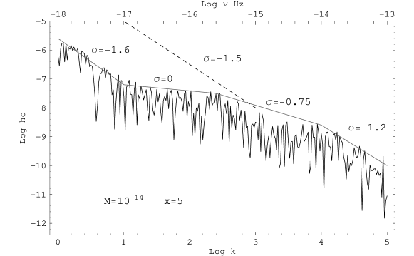
Figure 4: Low frequency region of the amplitude spectrum of primordial gravitational waves, calculated at $x=5$, for $M=10^{-14}$. The dashed line corresponds to the result expected from the step-eos assumption.

The spectrum has an almost null slope in the region $10^{1}\lesssim{\mathsf{k}}\lesssim 10^{2.4}$ while in $10^{2.4}\lesssim{\mathsf{k}}\lesssim 10^{4}$ its inclination is modified because of the variation of $\omega_{\mathrm{ef}}$. That feature is completely different of what is obtained from an step-eos. Modelling $\omega_{\mathrm{ef}}$ with a step-function (dashed line in figure 1), other authors Grishchuk (2001); Zhang et al. (2005); Boyle and Steinhardt (2005); Zhang et al. (2006) obtain a spectrum with $\sigma\approx-1.5$ for ${\mathsf{k}}<10^{3}$ Zhang et al. (2006). For comparison a dashed line is included in figure 4, corresponding to the slope obtained with the step-eos.

A last comment is concerned with the region $1<{\mathsf{k}}\lesssim 10$ of figure 4. The picture was taken in $x=5$ and so the modes within that region are in the threshold of the transition from “outside” to “inside” the horizon (${\mathsf{k}}\sim aH$). Since the thin-horizon simplification is not considered in this work, that region shows a transitory slope ($\sigma\approx-1.6$), that disappears for $x$ smaller than 5, as the modes enter the horizon. This characteristic is not perceptible in the previous illustration due to the scale.

V.4 During the accelerated expansion

Nearly all the modes are already inside the horizon when the accelerated expansion begins. For that reason, the shape of the spectrum remains constant and only the amplitude is altered in that phase. Figure 5 shows a narrow slice of the current spectrum, so that the effect of the different models of dark energy can be better observed.

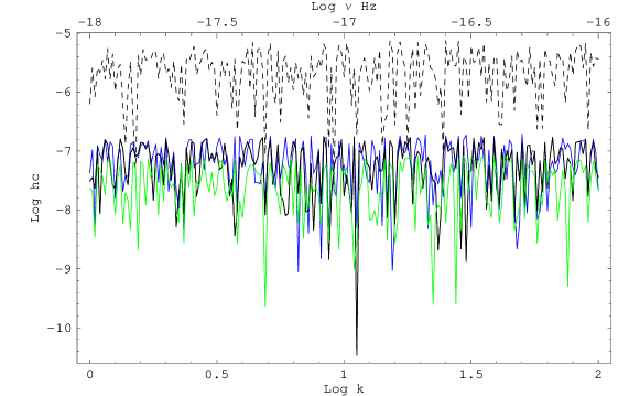
Figure 5: Present spectrum ($x=1$) of gravitational waves for $M=10^{-14}$. The dark energy models considered are: cosmological constant (solid), Chaplygin gas (blue), X-fluid (green), phantom (dashed), and quintessence (gray). The parameters used are the same as in figure 1.

The first characteristic to stress with regard to figure 5 is the complete degeneracy between cosmological constant and quintessence models ($\omega_{0}=-1,\omega_{1}=-0.2$), whose curves overlap completely. Moreover, the Chaplygin gas ($\bar{A}=0.8$ and $\alpha=1$) is also almost degenerate with those two curves. Observing figure 1 it is easy to notice that these three cases have very similar behavior and this degeneracy is expected. The X-fluid ($\omega=-0.8$), in turn, leads to an amplitude smaller than the cosmological constant while the phantom fluid ($\omega=-1.8$) acquires a larger amplitude. The difference is greater for phantom than non-phantom fluid because the chosen parameters are such that $|\omega_{X_{f}}-\omega_{\Lambda}|>|\omega_{X}-\omega_{\Lambda}|$. Since the dark energy begins to act very recently $x\sim 2$, the signature of different models is very weak – to produce a difference of $\approx 2$ in $\log{\mathsf{h}}_{c}$ scale, it is necessary to vary $\omega$ of almost one unit (the more negative is the equation of state, the larger is the amplitude).

Although just a particular choice of parameters is shown, other possible combinations have been tested. The results allow to state that: (1) for gCg Fabris et al. (2004); Soares-Santos et al. (2005a) the parameter $\alpha$ does not have any visible effect, while $\bar{A}$ increases the amplitude as it varies from $0$ (corresponding to the minimum stipulated by the spectrum without dark energy) to $1$ (reaching the $\Lambda$CDM curve); (2) the X-fluid Soares-Santos et al. (2005b) has only one parameter, $\omega$, that plays the same role of $\bar{A}$, but it assumes values more negatives than $-1$ and, in that case, the generated spectrum is above $\Lambda$CDM; (3) quintessence, in general, is completely degenerate with the X-fluid, unless that $\omega_{1}\sim 1$ (or greater) is assumed, but that does not have any physical sense for in this case the quintessence would affect the dynamics of the early Universe, being in contradiction with the most accepted cosmological models.

VI Search for empirical counterparts

VI.1 Direct attempts

The term “direct detection” should be strictly used only for experiments whose principle is to measure the deformation of the space-time submitted to tensor perturbations. The interferometric experiments lay in that class. However, it is common to include under that label detectors that measure the deformation of a proof mass in resonance and that is done in this work. The quantities $\Delta^{2}_{t}$, $\Omega_{gw}$ and ${\mathsf{h}}_{c}$ characterize, in an equivalent way, the gravitational wave background and do not depend on the detector. However, the signal $S(t)$ registered by an hypothetical detector will have a component $s(t)$, representing the observable, and another, the noise $r(t)$, which depends on the characteristics of the detector: $S(t)=s(t)+r(t)$. The mean (square) contribution of these components are Maggiore (2000):

$$\langle s^{2}(t)\rangle=\frac{F}{2}\int^{\infty}_{0}\nu^{-1}{\mathsf{h}}_{c}^{2}d\nu,\hskip 28.45274pt\langle r^{2}(t)\rangle=\int^{\infty}_{0}h_{r}^{2}d\nu,$$ (41)

where $F$ is an efficiency factor representing the loss of sensitivity due to the fact that gravitational waves come from all directions, while the detector is only maximally sensitive in some preferential ones. That expression for $\langle s^{2}(t)\rangle$ is valid for a stochastic background and the gravitational radiation may be considered detectable if

$${\mathsf{h}}_{c}>\sqrt{\frac{2\nu}{F}}h_{r}.$$ (42)

VI.1.1 Resonant masses

Schematically, a resonant mass detector is a (cylindrical or spherical) massive solid mass whose mechanical oscillations are excited by gravitational radiation and converted to electric sign by a sensor. The variation of the mass length is a sum of all its vibration modes, but the sensor is filtered to receive only the fundamental frequency, being therefore a narrowband detector.

In the case of a cylindrical bar, the efficiency factor is $F=8/15$, for the preferential direction of incidence is any direction perpendicular to the bar (if the sensor is located at one of its ends). The sensibility of the last generation experiments is Coccia (2000) $h_{r}\approx 10^{-22}\mathrm{Hz}^{-1/2}$, at $\sim 900$Hz. Using (42) the minimum detectable amplitude of those experiments is:

$${\mathsf{h}}_{c}\gtrsim 5,8\times 10^{-21},\hskip 28.45274pt{\mathrm{for}}\ \ {\mathsf{k}}\approx 4\times 10^{20}.$$ (43)

A spherical detector has a larger mass for the same resonance frequency implying in a greater cross-section. Besides, it is sensitive to different directions and polarizations of the incident radiation. The sensibility of those detectors is planned to be Aguiar et al. (2005) $h_{r}\approx 10^{-23}\mathrm{Hz}^{-1/2}$, for frequencies between $200$Hz and $2$kHz. Equation (42) here implies that resonant spheres are able to detect gravitational waves of up to

$${\mathsf{h}}_{c}\gtrsim 2,7\times 10^{-22},\hskip 28.45274pt\mathrm{for}\ \ {\mathsf{k}}\approx 1\times 10^{20}.$$ (44)

Comparing bars (43) and spheres (44), one notices an improvement of one order of magnitude, but that is still not enough to detect waves of cosmological origin.

VI.1.2 Interferometers

Laser interferometry is used in large detectors to measure the displacement of free-falling masses submitted to gravitational radiation. The basic components of those detectors are two arms of length $L$ connected at one end and three masses (one at the junction point, two at the free ends), constituting three pendulums. The preferential incident direction is perpendicular to the plan of the arms and $F=2/5\sin^{2}\theta$, where $\theta$ is the angle formed by the arms Maggiore (2000).

Unlike resonant masses, interferometers are broadband apparatus whose maximum wavelength is limited by the size of the arms. The main interferometric detectors are: LIGO Gustafson et al. (1999), with a 4km arm length; VIRGO Acernese et al. (2005a, b), 3km-sized; GEO600 Grote et al. (2005) and TAMA300 Ando and The TAMA Collaboration (2000), with 600 and 300 meters, respectively; AIGO/ACIGA McClelland et al. (2000), planned to have 4km; and finally, the most ambitious projects, BBO Corbin and Cornish (2006) and LISA Danzmann and Rüdiger (2003) are space interferometers where three arms ($5\times 10^{6}$km in LISA and $5\times 10^{5}$km in BBO) are arranged in an equilateral triangle.

The detectability estimate is performed using (42) once more. The results are shown in figure 6.

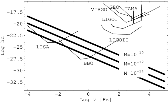
Figure 6: Gravitational wave spectrum for three inflationary energy scales ($M=10^{-14}$, $10^{-12}$, $10^{-10}$, from bottom to top, thick lines) in comparison with sensitive estimates for the detectors.

In the high frequency band, resonant masses and ground-based interferometers are shown, all with insufficient sensibility to detect primordial gravitational waves. The sensitivity curves of resonant masses are nearly reduced to a point in that scale, for these are, by construction, narrowband detectors. The interferometric detectors are also identified in the figure. Only LISA and BBO would be able to detect a cosmological signal, but both are still in project Corbin and Cornish (2006); Danzmann and Rüdiger (2003).

VI.2 CMB: an indirect attempt

In simple terms, one can say that Hu et al. (1997) until $z_{*}\approx 10^{3}$, the temperature of the Universe is high enough to ionize the hydrogen and, via Compton scattering, photons and electrons are coupled; in addition, electrons are also coupled to barions through electromagnetic interaction. The radiation pressure offers resistance to gravitational forces and acoustic oscillations arise in the plasma. In $z_{*}$, the hydrogen recombines (and the photons last scatter); the Universe becomes then transparent to photons and compression and rarefaction areas of the plasma at that redshift represent hot and cold areas, respectively; besides, photons suffer gravitational redshift when leaving the potential wells of the last scattering surface (Sachs-Wolfe effect Sachs and Wolfe (1967)). The resulting fluctuations appear as (primary) anisotropies in the sky.

The theoretical calculation of the CMB anisotropies is based on the linear theory of cosmological perturbations Giovannini (2005). The temperature anisotropy at position ${\bf x}$ and direction ${\bf n}$, $\Delta_{T}({\bf x},{\bf n})$, depends, in principle, on both the direction and the frequency, but the distortions in frequency are of second order. A Fourier expansion of $\Delta_{T}({\bf x},{\bf n})$, results in modes that propagate independently of each other. Assuming axial symmetry around ${\bf k}$, a Legendre expansion can also be done:

$$\Delta_{T}({\bf k},{\bf n})=\sum_{l}(2l+1)(-i)^{l}\Delta_{T_{l}}P_{l}(\mu),\hskip 28.45274pt\mu={\bf k}\cdot{\bf n}/k,$$ (45)

where $P_{l}(\mu)$ is the Legendre polynomial of order $l$, $\Delta_{T_{l}}$ is the associated multipole moment and $\Delta_{T}({\bf k},{\bf n})$ is the Fourier transform of $\Delta_{T}({\bf x},{\bf n})$. A similar expression can be written for polarization anisotropies $\Delta_{P}({\bf k},{\bf n})$.

The Boltzmann equation, which describes the temporal evolution of the Stokes parameters of the radiation field, is constituted by a collisional (referring to the Thompson scattering) and a non-collisional term. In the case of tensor perturbations, the resulting equation is Crittenden et al. (1993)

$${\Delta^{\prime}}_{T}^{(t)}+ik\mu\Delta_{T}^{(t)}=-h^{\prime}-\kappa^{\prime}\left(\Delta_{T}^{(t)}-{\bf Y}\right)$$

$${\Delta^{\prime}}_{P}^{(t)}+ik\mu\Delta_{P}^{(t)}=-\kappa^{\prime}\left(\Delta_{P}^{(t)}+{\bf Y}\right)$$ (46)

$${\bf Y}=\left[\frac{1}{10}\Delta_{T_{0}}^{(t)}+\frac{1}{35}\Delta_{T_{2}}^{(t)}+\frac{1}{210}\Delta_{T_{4}}^{(t)}-\frac{3}{5}\Delta_{P_{0}}^{(t)}+\frac{6}{35}\Delta_{P_{2}}^{(t)}-\frac{1}{210}\Delta_{P_{4}}^{(t)}\right]$$

where $h$ is governed by equation (9) and

$$\kappa=\int^{\tau_{0}}_{\tau}\kappa^{\prime}d\tau$$ (47)

represents the optical depth (and $\kappa^{\prime}\equiv an_{e}x_{e}\sigma_{T}$). The solutions of (46) may be written in the form Seljak and Zaldarriaga (1996)

$${\cal F}(k,\tau_{0})=\int^{\tau_{0}}_{0}e^{ik\mu(\tau-\tau_{0})}{\cal S}(k,\tau)d\tau.$$ (48)

where ${\cal F}$ is the (temperature or polarization) anisotropy, $\tau_{0}$ is the present time and ${\cal S}$ is the corresponding source term:

$${\cal S}_{T}^{(t)}=-e^{-\kappa}h^{\prime}+{\cal K}{\bf Y}\hskip 28.45274pt{\cal S}_{P}^{(t)}=-{\cal K}{\bf Y},$$ (49)

where ${\cal K}=\kappa^{\prime}\exp(-\kappa)$ is the visibility function. Expanding ${\cal F}$ in terms of tensor multipoles one has

$${\cal F}_{l}(k,\tau_{0})=\int^{\tau_{0}}_{0}\sqrt{\frac{(l+2)!}{2(l-2)!}}\ [k(\tau-\tau_{0})]^{-2}\ j_{l}[k(\tau-\tau_{0})]{\cal S}(k,\tau)d\tau\ .$$ (50)

If the observation takes place at ${\bf x}=0$, the expansion of ${\cal F}$ in spherical harmonics is

$${\cal F}=\sum_{l=0}^{\infty}\sum_{m=-l}^{l}a_{lm}Y_{lm}(\theta,\phi)=\frac{1}{(2\pi)^{3/2}}\int d{\bf k}{\cal F}_{l}\ ,$$ (51)

where $Y_{lm}$ is the angular part of the spherical harmonic eigenfunctions, such that:

$$P_{l}(\mu)=\frac{4\pi}{2l+1}\sum_{m=-l}^{l}Y_{lm}^{*}(\theta,\phi)Y_{lm}(\theta,\phi),\hskip 28.45274pt\mu=\cos\theta$$ (52)

¿From (52) and (51) it results

$$a_{lm}=\frac{(4\pi)(-i)^{l}}{(2\pi)^{3/2}}\int d{\bf k}\ {\cal F}_{l}\ Y^{*}_{lm}(\theta,\phi),\hskip 28.45274pt\langle a_{lm}a_{l^{\prime}m^{\prime}}^{*}\rangle\equiv C_{l}\delta_{ll^{\prime}}\delta_{mm^{\prime}}\ .$$ (53)

The evolution of the Boltzmann equations does not depend on ${\bf k}$, so it is possible to take Ma and Bertschinger (1995), ${\cal F}_{l}\rightarrow h_{\mathrm{ini}}{\cal F}_{l}$, where $h_{\mathrm{ini}}$ is the initial condition of the perturbation. The correlation function is $\langle h_{\mathrm{ini}}({\bf k})h_{\mathrm{ini}}^{*}({\bf k}^{\prime})\rangle=\Delta_{t}^{2}(k)\delta({\bf k}-{\bf k}^{\prime})$ and so the $C_{l}$ coefficients are determined:

$$C_{l}^{(t)}=\left[\frac{4\pi}{(2\pi)^{3/2}}\right]^{2}\int\Delta^{2}_{t}|{\cal F}_{l}|^{2}\langle Y_{lm}^{*}Y_{lm}\rangle d{\bf k}=\frac{2}{\pi}\int\Delta^{2}_{t}|{\cal F}_{l}|^{2}k^{2}dk$$ (54)

In short, to calculate the induced tensor perturbations of the temperature (polarization) $C_{l}$ spectrum it is necessary to compute the multipoles $\Delta_{T_{l}}^{(t)}$ ($\Delta_{P_{l}}^{(t)}$) using (50) and the source term ${\cal S}_{T}^{(t)}$ (${\cal S}_{P}^{(t)}$); the result is applied directly on (54), using the initial power spectrum $\Delta_{t}^{2}$, given by equation (17) and shown in figure 2. All information on the evolution of gravitational waves after inflation is contained in the source terms.

From (49) it is noticed that the polarization source term is suppressed if the media is optically thin, so that after reionization the polarization due to gravitational waves is negligible and the polarization spectrum may be used to verify the initial conditions obtained in section IV.2.1. Although both tensor and scalar perturbations affect the CMB, it is possible to find a mode ($B$ polarization mode) which is induced only by gravitational waves and this is a promising future perspective to constraint the initial conditions of the problem.

The temperature source term in (49) is reduced to ${\cal S}_{T}^{(t)}\approx-h^{\prime}$ after recombination and, therefore, it contains information about the evolution of the power spectrum since then. Moreover, after the condition $k\ll aH$ is achieved the amplitude $h$ falls as $a^{-1}$ and only the modes $k\lesssim k_{*}$ (where $k_{*}$ is the wavelength of the order of the Hubble radius at recombination time) contribute to the source term ${\cal S}_{T}^{(t)}$.

The power spectrum of temperature anisotropies was calculated according to the prescription above, using the profiles of $\kappa$ and ${\cal K}$ obtained from the Saha equilibrium equation and the envelope of the spectrum corresponding to the $\Lambda$CDM model with $M=10^{-14}$. The integration limits ($k_{\mathrm{min}}=1$ and $k_{\mathrm{max}}=1500\simeq k_{*}$, $x_{\mathrm{min}}=1$ and $x_{\mathrm{max}}=1500$) were chosen in order to reduce the computacional cost without losing relevant information. Only the multipoles $l\leq 10$ were calculated and the result is a plane spectrum, with amplitude $C_{l}l(l+1)/2\pi=41.1(\mu\mathrm{K})^{2}$. The form of the spectrum is compatible with other theoretical predictions Crittenden et al. (1993); Efstathiou and Chongchitnan (2006), as well as with observational results Spergel et al. (2006), but the value found is $\sim 25$ times lower. This means that the inflationary energy scale $M$ could be larger than the conservative limit adopted along this work. With $M=10^{-10}$, this difference is suppressed: $C_{l}l(l+1)/2\pi=1.01\times 10^{3}(\mu\mathrm{K})^{2}$. The current spectrum of gravitational waves can have in this case the amplitude given by the superior curve of figure 6.

The limit $M=10^{-14}$($E_{\mathrm{inf}}=10^{-3,5}m_{Pl}$) is a direct consequence of the condition that the amplitude of tensor perturbations should not be larger than the observed CMB anisotropies and, at a first glimpse it may seem in contradiction with the result presented above. Under a more careful glance, however, one notices that this last result is obtained when considering the physical processes involved in the generation of anisotropies induced by gravitational waves. Additional physical ingredients (specifically the ones regarding to the recombination process) that determine the efficiency with which the perturbations imprint themselves on the CMB spectrum had to be considered. In order to avoid the additional uncertainties introduced by these new ingredients, the authors have chosen the most conservative limit, $M=10^{-14}$, when performing the analyzes of section V.2. However, other possible values have been considered in the literature between $M\simeq 10^{-8}$ Kolb and Tuner (1990) and $M\simeq 10^{-11}$ Efstathiou and Chongchitnan (2006), which are consistent with the results here presented.

VII Summary and conclusions

The origin and evolution of the primordial gravitational wave background was computed for different cosmologies. Temporal evolution of these relics is governed by an oscillator-like equation with an exciting potential $a^{\prime\prime}/a$. The initial conditions are set-up during inflation and, for a de Sitter model, the initial spectrum is flat. As the modes cross back to the horizon, ever since the end of inflation until $x\sim 10^{4}$, the spectrum assumes a slope ($\sigma\approx-1.2$) in the high frequency region (${\mathsf{k}}>10^{4}$). That slope is maintained in the subsequent eras. The modes with ${\mathsf{k}}$ between $\sim 10^{4}$ and $\sim 10^{2}$ ($\sigma=-0.75$) enter the horizon during the radiation-matter transition and the step-eos assumption is shown to be unsupported in these redshifts. The final spectrum is flat in the low frequency band $1\leq{\mathsf{k}}\lesssim 100$.

The analysis here accomplished also shows that gravitational waves are not strongly affected by dark energy. Establishing constraints on dark energy using gravitational waves is not a promising task (even though one could arrive to the very opposite conclusion naïvely considering that both of them interact only via gravitation). One must measure the gravitational wave spectrum with precision better than $\delta_{{\log}_{10}{\mathsf{h}}_{c}}\lesssim 0,4\%$ to constrain $\omega$ within $\delta_{\omega}<1\%$ (with the energy scale $M$ independently fixed and an X-fluid equation of state assumed a priori).

Once obtained the theoretical spectrum of cosmic gravitational waves, the natural question concerns the empiric counterparts of those forecasts. None among all the already built experiments is sensitive enough to detect primordial gravitational waves, because at their operational frequencies that signal is orders of magnitude below their noise levels. The perspectives are promising for the future space detectors though.

CMB, in turn, supplies a concrete possibility of obtaining this information indirectly, but the influence of gravitational waves on the CMB must be understood in detail in order that one can be able to extract information from the angular spectra whose detection is expected to be greatly improved in the near future. The calculation here performed establishes a limit on the energy scale of inflation: $M\lesssim 10^{-10}$.

This work was financially supported by FAPESP and CNPq.

References

- Einstein (1916) A. Einstein, Sitzungsberichte der Königlich Preußischen Akademie der Wissenschaften (Berlin), Seite 688-696. p. 688 (1916).
- Taylor et al. (1976) J. H. Taylor, R. A. Hulse, L. A. Fowler, G. E. Gullahorn, and J. M. Rankin, Astrophys. J. Lett. 206, L53 (1976).
- Gullahorn and Rankin (1978) G. E. Gullahorn and J. M. Rankin, Astrophys. J. 83, 1219 (1978).
- Grishchuk (2005) L. P. Grishchuk (2005), eprint gr-qc/0504018.
- Zhang et al. (2005) Y. Zhang, Y. Yuan, W. Zhao, and Y.-T. Chen, Class. Quantum Grav. 22, 1383 (2005).
- Zhang et al. (2006) Y. Zhang, X. Z. Er, T. Y. Xia, W. Zhao, and H. X. Miao, Class. Quantum Grav. 23, 3783 (2006), eprint astro-ph/0604456.
- Efstathiou and Chongchitnan (2006) G. Efstathiou and S. Chongchitnan (2006), eprint astro-ph/0603118.
- Mukhanov et al. (1992) V. F. Mukhanov, H. A. Feldman, and R. H. Brandenberger, Phys. Rep. 215, 203 (1992).
- Maldacena (2003) J. Maldacena, JHEP 305, 13 (2003), astro-ph/0210603.
- Giovannini (2005) M. Giovannini, Int. J. Mod. Phys. D 14, 363 (2005), eprint astro-ph/0412601.
- Weinberg (1972) S. Weinberg, Gravitation and Cosmology (John Wiley, New York, 1972).
- Boyle and Steinhardt (2005) L. A. Boyle and P. J. Steinhardt (2005), eprint astro-ph/0512014.
- Kolb and Tuner (1990) E. W. Kolb and M. S. Tuner, The Early Universe (Addison-Wesley, Reading, Massachusetts, 1990).
- Coles (2005) P. Coles, Nature 433, 248 (2005).
- Copeland et al. (2006) E. J. Copeland, M. Sami, and S. Tsujikawa (2006), eprint hep-th/0603057.
- Lima (2004) J. A. S. Lima, Braz. J. Phys. 34, 194 (2004).
- Caldwell (2002) R. R. Caldwell, Phys. Lett. B 545, 23 (2002).
- Grishchuk (2001) L. P. Grishchuk, Lect. Notes Phys. 562, 167 (2001).
- Grishchuk (2003) L. P. Grishchuk (2003), eprint gr-qc/0305051.
- Maia (1993) M. R. G. Maia, Phys. Rev. D 48, 647 (1993).
- Baskaran et al. (2006) D. Baskaran, L. P. Grishchuk, and A. G. Polnarev (2006), eprint gr-qc/0605100.
- Lyth and Riotto (1999) D. Lyth and A. Riotto, Phys. Rep. 314, 1 (1999), eprint hep-ph/9807278.
- Fabris et al. (2004) J. C. Fabris, S. V. B. Gonçalves, and M. Soares-Santos, Gen. Rel. Grav. 36, 2559 (2004).
- Soares-Santos et al. (2005a) M. Soares-Santos, S. V. B. Gonçalves, J. C. Fabris, and E. M. de Gouveia Dal Pino, in Magnetic Fields in the Universe: from laboratory and stars to primordial structures, edited by E. M. DE GOUVEIA DAL PINO, G. Lugones, and A. Lazarian (AIP Conf. Procs., New York, 2005a), vol. 784, p. 800.
- Soares-Santos et al. (2005b) M. Soares-Santos, S. V. B. Gonçalves, J. C. Fabris, and E. M. de Gouveia Dal Pino, Braz. J. Phys. 35, 1191 (2005b).
- Maggiore (2000) M. Maggiore, Phys. Rep. 331, 283 (2000).
- Coccia (2000) E. Coccia, in Meshkov (2000), p. 32.
- Aguiar et al. (2005) O. D. Aguiar et al., Class. Quantum Grav. 22, 209 (2005).
- Gustafson et al. (1999) E. Gustafson, D. Shoemaker, K. Strain, and R. Weiss (1999), URL http://www.ligo.caltech.edu/docs/T/T990080-00.pdf.
- Acernese et al. (2005a) F. Acernese et al., in General Relativity and Gravitational Physiscs: 16th SIGRAV Conference on General Relativity and Gravitational Physics, edited by G. Vilasi, G. Espositio, G. Lambiase, G. Marmo, et al. (AIP Conf. Procs., New York, 2005a), vol. 751, p. 92.
- Acernese et al. (2005b) F. Acernese et al., Class. Quantum Grav. 22, 185 (2005b).
- Grote et al. (2005) H. Grote et al., Class. Quantum Grav. 22, 193 (2005).
- Ando and The TAMA Collaboration (2000) M. Ando and The TAMA Collaboration, in Meshkov (2000), p. 128.
- McClelland et al. (2000) D. E. McClelland et al., in Meshkov (2000), p. 140.
- Corbin and Cornish (2006) V. Corbin and N. J. Cornish, Class. Quantum Grav. 23, 2435 (2006).
- Danzmann and Rüdiger (2003) K. Danzmann and A. Rüdiger, Class. Quantum Grav. 20, 51 (2003).
- Hu et al. (1997) W. Hu, N. Sugiyama, and J. Silk, Nature 386, 37 (1997), eprint astro-ph/9604166.
- Sachs and Wolfe (1967) R. K. Sachs and A. M. Wolfe, Astrophys. J. 147, 73 (1967).
- Crittenden et al. (1993) R. Crittenden, J. R. Bond, R. L. Davis, G. Efstathiou, and P. J. Steinhardt, Phys. Rev. Lett. 71, 324 (1993).
- Seljak and Zaldarriaga (1996) U. Seljak and M. Zaldarriaga, Astrophys. J. 469, 437 (1996), eprint astro-ph/9603033.
- Ma and Bertschinger (1995) C.-P. Ma and E. Bertschinger, Astrophys. J. 455, 7 (1995).
- Spergel et al. (2006) D. N. Spergel et al. (2006), eprint astro-ph/0603449.
- Meshkov (2000) S. Meshkov, ed., Gravitational Waves: Third Edoardo Amaldi Conference, vol. 523 (AIP Conf. Procs., New York, 2000).