The SuperWASP wide-field exoplanetary transit survey: Candidates from Fields 23hr RA 03hr
Abstract
Photometric transit surveys promise to complement the currently known sample of extra-solar planets by providing additional information on the planets and especially their radii. Here we present extra-solar planet (ESP) candidates from one such survey called, the Wide Angle Search for Planets (WASP) obtained with the SuperWASP wide-field imaging system. Observations were taken with SuperWASP-North located in La Palma during the April to October 2004 observing season. The data cover fields between 23hr and 03hr in RA at declinations above +12. This amounts to over 400,000 stars with V magnitudes 8 to 13.5. For the stars brighter than 12.5, we achieve better than 1 percent photometric precision. Here we present 41 sources with low amplitude variability between 1 and 10 mmag, from which we select 12 with periods between 1.2 and 4.4 days as the most promising extrasolar planet candidates. We discuss the properties of these ESP candidates, the expected fraction of transits recovered for our sample, and implications for the frequency and detection of hot-Jupiters.
keywords:
methods: data analysis – planetary systems – stars: variables: other1 Introduction
The discovery of the large debris disk around Pic (Smith & Terrile, 1984) and other young stellar sources with disks (Jayawardhana et al., 1998; Lecavelier Des Etangs et al., 1997), plus the subsequent discovery of numerous extra-solar planets (ESP) has led to a resurgence in the study of planet and solar system formation. Discoveries of ESPs have been dominated by radial velocity surveys (Mayor & Queloz, 1995; Marcy & Butler, 1998, 2000; Udry et al., 2000). Currently, there are over 170 known ESPs orbiting around over 150 host stars. Photometric transit surveys have identified about 10 new planets, starting with: the confirmation of the first system, HD 209458b (Henry et al., 2000; Charbonneau et al., 2000), followed by several discovered with the OGLE project and confirmed with radial velocity follow-up (Konacki et al., 2003, 2004; Pont et al., 2004; Bouchy et al., 2005; Konacki et al., 2005), to the discovery of TrES 1 (Alonso et al., 2004), the detection of the transits from the radial-velocity discovered HD 189733 (Bouchy et al., 2005), and the recent discovery and follow-up of XO-1b (McCullough et al., 2006; Wilson et al., 2006). These planets typically have periods less than 4 days, orbital distance 0.05 AU, and Jupiter-like masses and radii, and hence have been called the hot-Jupiters. Additionally, several very short period (P 1.5 d) systems have been discovered (Konacki et al., 2003; Bouchy et al., 2004) and termed very-hot-Jupiters.
Radial velocity (RV) surveys measure the Doppler velocity of individual stars at many different times, which is a very time consuming procedure. The photometric transit method can measure thousands of stars simultaneously. In addition to monitoring a large number of stars, photometric transit detections provide information on the planet’s radius and inclination, not readily available from RV surveys. It is currently not know what fraction of stars contain planets. The fraction of planets that may be hot-Jupiters is also not known. About 20% of the currently known ESPs have periods less than 10 days (Butler et al., 2006) and 10-15% of solar-type stars surveyed have ESPs (Lineweaver & Grether, 2003). There have been several attempts to better define what percentage of stars have planets. These range from 1-2% (Brown, 2003) to 20% (Lineweaver & Grether, 2003), but the latter also speculate this may be a lower limit. The large number of stars covered by photometric transit surveys should provide better constraints on the fraction of stars with hot-Jupiters, and may shed light on their formation mechanisms.
Here we present results from one such photometric transit survey, called WASP (the Wide Angle Search for Planets). WASP consists of 2 separate telescopes, called SuperWASP North (SW-N) and SuperWASP South (SW-S). The SuperWASP telescopes were designed to cover a large field-of-view with better than 1% photometric accuracy down to 12th magnitude. Each SW telescope consists of 8 separate cameras, each of which covers 61 sq degrees of sky, and the combined system surveys nearly 500 sq degrees. The results presented here are from the 2004 SW-N observing campaign taken with a 5 camera configuration. A description of the SW instruments and observing strategy are presented in § 2. In § 3 we present the data reduction and analysis techniques for the ESP search. Candidates with secure low amplitude variability that may be ESPs are presented in § 4. In § 5, we discuss possible false alarms, expected fraction of recovered transits, and indications for the frequency of hot-Jupiters, their properties and observing follow-up strategies to confirm the transits planetary nature. Lastly, in § 6 we summarize our findings.
2 Instrumentation and Observations
2.1 Instrumentation
The SuperWASP (SW) telescopes were designed to cover a large area of sky and achieve photometric accuracy of a few millimags, and improve on the success of the prototype WASP0 instrument (Kane et al., 2004, 2005). SW N in La Palma is contained in its own custom enclosure with a hydraulically operated roll-away roof, and its own GPS and weather station (Christian et al., 2005; Pollacco et al., 2006). The telescope mount is a rapid slew fork mount (10o/sec) from OMI, Inc. Commercially available components were used where available to keep costs down and decrease construction time. These components include: the telescope control system (TCS), a dedicated PC for each camera for data acquisition, and a PC attached to a tape (DLT) autoloader for data storage. The TCS monitors the weather, sets time for the FITS data header from the GPS and can close the roof in the event of a weather alert (Pollacco et al., 2006). All major components are run with Linux OS.
To meet the science requirements of covering a large area of sky with high photometric precision, a combination of Canon 200-mm f/1.8 lenses and Andor e2v 2k2k back illuminated CCDs was chosen. The CCDs are passively cooled with a Pelletier cooler and have a very short 4-sec readout time. This combination of lens and camera gives a field of 7.8o 7.8o (61 sq degrees). No additional filters were used and this ”wide-V” set-up covers from 8–15 magnitude for a typical 30 second exposure. A 1% photometric precision was obtained for magnitudes brighter than V=12.5. Additional details of the SuperWASP project and instrumentation is presented in Pollacco et al. (2006).
2.2 Observational Strategy
SW-N was commissioned in November 2003, and inaugurated on 16 April 2004. Our initial observing strategy was tailored toward searching for extra-solar planet transits. This was to observe fields with a large number of stars, but to avoid the Galactic plane where over-crowded fields would increase the number of blended stars and make detection and data reduction difficult. Based on the Besancon Galactic model (Robin et al., 2003 and references therein) a declination of +28 was chosen, with the telescope stepping through RA in 1 hour increments centered on the current LST, but within the 4.5 hr hour angle limit of the mount. A maximum of 8 fields were observed with a duration of 1 minute per field, including a 30 second exposure, 4 second read-out and the time for the telescope to slew and settle at the new field. Such observations provide well sampled light curves with a cadence of better than 8 minutes between subsequent measurements. This observing strategy provides a nightly baseline of over 6 hours of coverage for the 6 fields centered near LST at midnight, and over 4 hrs of coverage on 10 fields per night. A typical field contains 20,000 stars per camera at magnitudes brighter than 13. Nightly calibrations, such as bias levels, darks, and flat fields to remove the pixel-to-pixel variations and vignetting were obtained using automated scripts. Biases and flat fields were obtained at the beginning and end of each night, and flat fields were taken during twilight with the telescope pointed at zenith and the drive off. Exposure times were initially based on the data in Tyson & Gal (1993) and adjusted from the counts in the first image.
The 150 nights from the 2004 observing season covered several dozen separate fields and resulted in the detection of slightly more than 6.7 million stars. For the extra-solar planet search these observations were separated into 6 equal sections of the sky, each containing about 1 million stars. This work presents the stars from 23hr RA 03hr, and contains nearly 900,000 stars observed for at least 25 nights and 400 image frames. The statistics for the observed fields are presented in Table 1, and the distribution of all stars in our sample as a function of SW-N V magnitude is shown in Figure 1. Approximately 400,000 stars are brighter than 13.5 magnitude.
| Field | Nights | Images | Stars |
|---|---|---|---|
| SWASP J | |||
| 2317+2326 | 115 | 4882 | 38993 |
| 2343+3126 | 112 | 4569 | 51694 |
| 2344+2427 | 92 | 3406 | 38332 |
| 2344+3944 | 110 | 4539 | 59202 |
| 0016+3126 | 111 | 4525 | 48448 |
| 0017+2326 | 110 | 4501 | 36676 |
| 0043+3126 | 29 | 406 | 38458 |
| 0044+2127 | 61 | 2046 | 30156 |
| 0044+2427 | 29 | 406 | 34267 |
| 0044+2826 | 80 | 3088 | 40578 |
| 0045+3644 | 80 | 3061 | 46856 |
| 0115+2826 | 79 | 3063 | 33249 |
| 0116+2027 | 78 | 3051 | 27183 |
| 0116+3126 | 28 | 372 | 34276 |
| 0117+2326 | 27 | 371 | 28312 |
| 0143+3126 | 72 | 2591 | 36623 |
| 0144+2427 | 52 | 1576 | 28059 |
| 0144+3944 | 71 | 2570 | 56242 |
| 0216+3126 | 71 | 2560 | 40368 |
| 0217+2326 | 70 | 2559 | 30535 |
| 0243+3126 | 61 | 1883 | 40191 |
| 0244+2427 | 42 | 1017 | 28958 |
| 0244+3944 | 60 | 1879 | 78643 |

3 Analysis
3.1 Pipeline
We have constructed a custom data reduction pipeline, with a goal of obtaining millimag photometric precision for stars with V 12. The pipeline (only briefly described here) uses custom FORTRAN programs combined with shell scripts and several STARLINK packages, and creates master biases, darks, and flat fields for each night of observations. Flat field calibration frames from individual nights are combined into a master flat using an exponential weighting with the contribution of flats older than 14 days diminishing (Collier-Cameron et al., 2006). Each science exposure is bias subtracted, dark corrected, flat fielded, and the astrometric solution is computed using reference stars from the USNO-B1.0 and Tycho catalogs.
Aperture photometry is performed on the final calibrated images with a custom-built package tailored to deal with the ultra-wide fields. Bad pixel masks are applied to each frame, and a blending index is assigned for every object detected. The blend index is defined as the ratios of the fluxes in various sized apertures for an individual star (Pollacco et al., 2006). We define two blend indices based on the flux ratios: and , where , , are the fluxes measured in apertures of 2.5, 3.5, and 4.5 pixels, respectively. Removing night-to-night variations in air-mass and sky conditions was difficult, but the aperture photometry does achieve slightly better than the required 1% precision at V=12.5. For the transit searching, additional systematic errors are removed with the SysREM algorithm (Tamuz et al., 2005). RMS precision as a function of SW magnitude are shown in Collier-Cameron et al. (2006) and Pollacco et al. (2006). Fluxes are computed in the 3 mentioned above apertures and output, along with other source attributes to a FITS binary table. The final pipeline data products include the calibrated images, catalog information, and time-tagged photometric data for each star. Trends (such as extinction) are removed from the data, and the binary table is ingested by the archive. A list of all cataloged targets is compiled from the ingested FITS tables and compared with the WASP catalogue. New objects are given IAU-compatible names, and all objects are assigned to a 5 sky tiles based on their coordinates. Photometric data are split from the input files and stored as intermediate per-sky-tiles. Photometric points within each sky-tile are re-ordered to ensure that they are in consecutive rows for a given star. These files are registered within the archive data-base management system (DBMS) along with their names, location, and various meta-data. The archive can then be interrogated and the photometric data extracted as a single, coherent per-object light curve for longer term temporal analysis. The object catalog is expected to increase by objects per year. This public archive is hosted at Leicester within LEDAS (Leicester Database and Archive Service).
3.2 Transit Searching
The large number of stars makes visual inspection of every light curve unfeasible. For this reason the transit searching programs provide rank ordered lists of the best light curves based on derived transit depth, signal-to-noise, and for periods less than 5 days. Another important and effective parameter in culling the list of candidates was the signal-to-red noise, (Sred). Sred is the ratio of the best fit transit depth to RMS scatter and is described in detail in (Collier-Cameron et al., 2006). Our refined list of candidates can then be inspected visually for further analysis. Light curves that show unusual extinction variations or other systematic problems can then be eliminated. Once the spurious candidates are culled from the master list further analysis of the light curves is undertaken.
There are several well used transit detection algorithms (Tingley et al., 2003; Moutou et al., 2005). These include the box-shaped searches, such as, the Box-fitting Least-Squares (BLS) algorithm (Kovács et al., 2002), matched filter algorithms (Kay, 1998), and Bayesian techniques (Defaÿ et al., 2001; Aigrain & Favata, 2002). We have applied an improved BLS algorithm to the 2004 data to search for transits. This method is described in detail in a companion paper by Collier-Cameron et al. (2006). BLS allows fast and efficient searching for transits, while keeping the false alarm rate low. Additionally, Moutou et al. (2005) suggest that the BLS method was preferable in a comparison of several commonly used algorithms. An extensive comparison of the leading transit detection algorithms as applied to SuperWASP data is currently underway (Enoch et al., 2006).
Several additional techniques were adopted to the transit finding software to keep the false alarm rate low. These include a test for ellipsoidal variations in the light curve, such as would be produced by close stellar eclipsing binary systems. The amplitude of the ellipsoidal variations, (S/N)ellip, is also given for each system. Similar methods applied to OGLE candidates were successful in distinguishing stellar sources from true ESP candidates (Sirko & Paczyński, 2003). Additionally, true ESP transit light curves should be flat at the phase 180 away from the transit, at phase 0.5, the ’anti-transit’. Hence tests for the variability at phase 0.5 (Burke et al., 2006) were also added. We present our results for this set of SW data in the next section. From these and further scrutiny to distinguish low amplitude stellar systems from true ESPs we cull our list of extra-solar planet candidates.
4 Results
Systems that have good signal-to-noise and transit depths less than 10% are presented in Table 2. Here we have excluded systems showing secondary eclipses in their light curves and stars with any brighter neighboring stars within a 48 radius. We will apply strict criteria to the sources listed in the table to separate the stellar systems from the possible ESPs. Systems likely to be low stellar mass binaries are interesting in their own right and if confirmed would add valuable information to the Mass-Radius relations for low mass stars, and are thus included here. However, our current analysis does not allow us to give an accurate estimate of the binary fraction of the SuperWASP fields. Our transit searching methods were optimized for finding transit-like events, and many types of binaries (those with large changes in magnitude (10%) or large ellipsoidal amplitudes) are not reported. Thus, any estimate would only provide a lower limit to the true binary fraction, and this investigations is left for future publications.
4.1 ESP Candidate Selection
In the present work we are interested in the best possible ESP candidates and require these to have: (i) high signal-to-noise light curves (S 7), (ii) a reasonable transit depth for spectral type, (iii) a reasonable transit duration, with 1.3, where is the ratio of the observed transit duration to that expected based on the stellar and planetary radii (Tingley & Sackett, 2005), (iv) a flat bottomed transit shape, (v) to have been observed for at least 3 transits, and (vi) an ellipsoidal amplitude less than 5. Later type main-sequence dwarf stars will have deeper eclipses, and transits depths may be as large as 20%. Most hot-Jupiters have periods less than 10 days, which thus limits the transit duration to 7 hrs (Kane et al., 2005). A grazing angle transiting ESP may show a ’V-shaped’ transit, but in most cases this shape would indicate a grazing incidence eclipsing stellar system, and these types of transits are further scrutinized.
In order to estimate the size of the transiting planet, the size of the host star must also be determined. Several colour-temperature relations were used to constrain spectral types and stellar temperatures. The VSW and USNO B1 and R1 magnitude are available for all stars in our sample, and Tycho B and V plus 2MASS J, H, and K were used when available. Relations between VSW - K and temperature were derived using a coarse grid of V and K colours from a selection of 30,000 stars from Ammons et al. (2006). Subsequently, the stellar radii were determined from the derived stellar temperatures using J-H colors and the relation from Gray (1992). This relation was further optimized with a polynomial fit for the FGKM temperature range. No reddening correction was included in VSW - K. In general, with SuperWASP observations are away from the Galactic plane, the reddening correction should be small, but would serve to increase V-K and artificially lower the derived stellar radii. In Figure 2., we show a histogram of stellar radii for a sample of 2,000 stars (ones having all of the appropriate colours) selected from all fields and returned from the transit search code as having ’transit-like’ variability. The large peak in the figure at radii between 0.6 and 0.8 R☉ corresponds to the late K and M0 stars from the faint end of the SuperWASP data.

We derived a planet’s radius using the estimated stellar radius and a simple geometric transit model. The transit depth, F, is related to the ratio of the area of the planet to that of the star with the equation:
| (1) |
where F is the baseline flux of the star, and Rp and Rs are the radius of the planet and star, respectively. Planetary radii in Table 3 are given in units of Jupiter-radii using the above relation from (Tingley & Sackett, 2005), and the table also includes .
Additionally, we further refined the spectral type and host star’s radii using 2MASS colours to distinguish between dwarfs and giants. Similar transit depths for non-main sequence stars would imply radii larger than that of Jupiter-sized planets. The 2MASS J-K color index is also presented in Table 3, and we compare the transit depths to infrared colors in Figure 3. JK has been shown to be a powerful tool in distinguishing dwarfs from giants (Brown 2003). Values of JK 0.7 are a strong indication that the star is a giant, and hence the observed transit is caused by a body much larger than a Jupiter-sized ESP. Or in some cases the giant may be diluting the eclipse of a stellar binary, and also be an imposter. The 3 sources excluded as ’Giants’ are over-plotted with filled circles.
4.2 ESP Transit Candidates
The above criteria, (presented in § 4.1) were rigorously applied to our selection of the best low amplitude sources. This leaves us with 12 good ESP candidates. Good ESP candidates are noted in bold face and commented as ESPc in Table 3. Over-plotted in Figure 3 are the theoretical curves for 0.5, 1.0 and 1.5 Jupiter radii planets. It can be seen many of these source’s transits have reasonable planetary radii between 0.5 and 1.5 RJ, and our best candidates are indicated by a filled symbol. Other sources in the figure have large ellipsoidal variation or have large derived planetary radii (Rp 1.9 RJ), and hence have been eliminated.

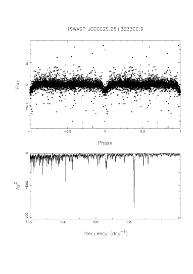
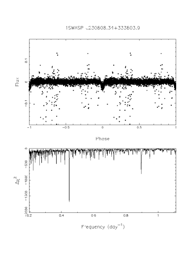
We now discuss several of the sources that were not chosen as ESP candidates and those reasons, and we then discuss the properties of the best ESP candidates individually. Light curves and periodograms for these sources are shown in Figures 4–17. Periodograms are included to show the robustness of the period searches and are discussed for unusual cases.
Several sources presented in Table 2 had ellipsoidal amplitudes great than 5, although several of these sources had reasonable planetary radii. We eliminated these as extra-solar planet candidates and these are noted as Ellip. large in Table 3. 1SWASP J000029.25+323300.9 and 1SWASP J230808.34+333803.9 are two such sources and their folded light curves and periodograms are shown in Figures 4 and 5.
Three sources that had derived planetary radii below 0.8 RJ and also passed most criteria, including a low ellipsoidal magnitude, but may very well be giant and not dwarf stars. These 3 stars, 1SWASP J002728.02+284649.2, 1SWASP J013452.76+293626.5, and 1SWASP J231302.08+262724.3 have JK greater than 0.7. These stars also have very large values for and this may also indicate the object causing the transit is indeed stellar.
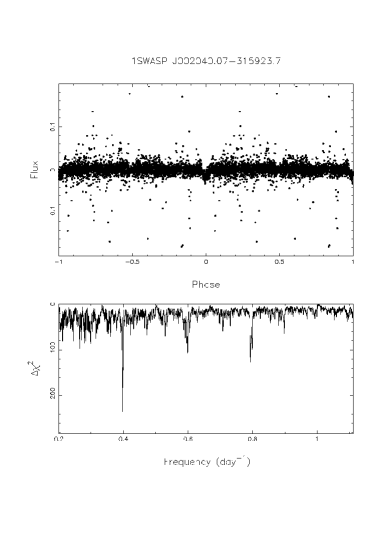
1SWASP J002040.07+315923.7 A total of 9 transits were detected for this system, and the periodogram shows a well determined period of 2.55 days (Figure 6). We classify this as a G1 star using colour and temperature relations. This gives a planet radius of 1.2RJ. Although the transit is clearly visible in its light curve, there are several faint sources within the SW aperture and blending can not be ruled out.
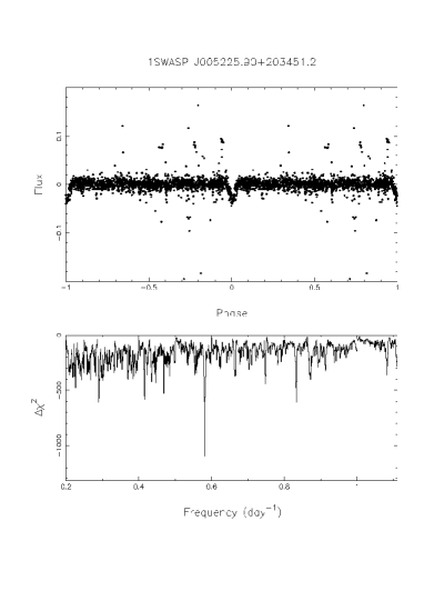
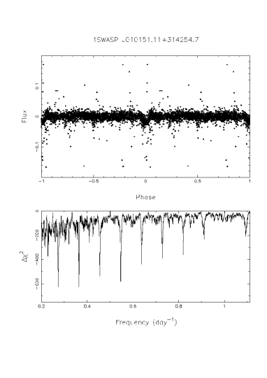
1SWASP J003039.21+205719.1, 1SWASP J005225.90+203451.2, and 1SWASP J010151.11+314254.7 were each observed in 2 different cameras. Although their light curves and periodograms show some scatter, nearly identical transit depths and periods were derived for each star from both of their observations. Their folded light curve and timing information are shown in Figure 7–9. The planetary radii derived for these objects range from 1.2–1.4 RJ, and the latter two stars have ellipsoidal amplitudes slightly greater than 3, and these may indeed be stellar systems. However, their ratios of the observed to theoretical transit durations () are reasonable.
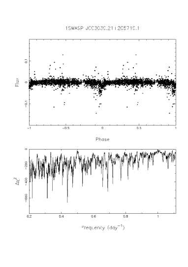
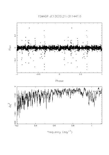
With a period of 4.4 days, 1SWASP J013033.21+311447.0 is one of the longer period candidates. Although its folded light curve shows a well defined transit, its periodogram (Figure 10) has excess scatter and additional photometric data would be beneficial. We derived a reasonable planetary radius of 1.07RJ for its G4 spectral type.
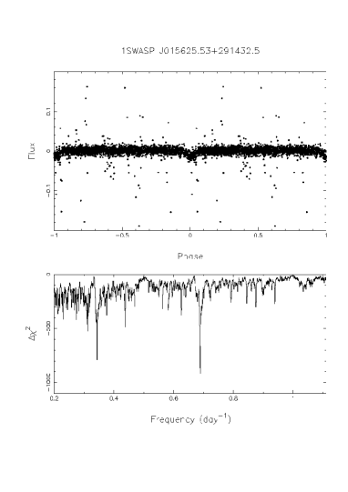
1SWASP J015625.53+291432.5 The observed short period for this system (1.45 days) may place it in the class of very-hot-Jupiters. Its periodogram, showing a well defined period, and light curve are presented in Figure 11. However, the transit depth is relatively shallow for a 0.7RJ planet and it has a large , making it more likely to be a grazing incident eclipsing stellar system or diluted by another star. There is another object within the SW aperture making the later scenario more likely. We note this as a marginal ESP candidate.
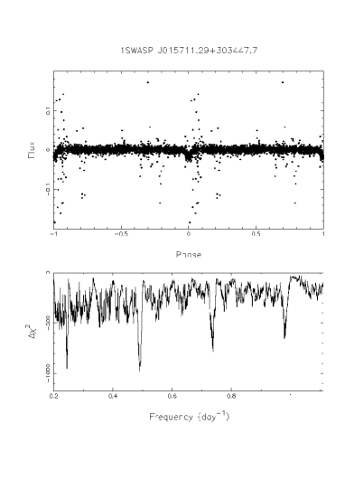
1SWASP J015711.29+303447.7 The light curve for this system is flat with a well pronounced transit (Figure 12). We derived a planet radius of 1.37RJ for its derived spectral type of F6. The expected transit duration is reasonable and this is a good ESP candidate worth further follow-up.
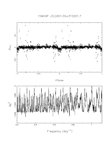
1SWASP J022651.05+373301.7 The short period of 1.2 days (Figure 13) may make this a very-hot-Jupiter, but its periodograms shows excess scatter and additional photometric measurements are needed to improved the period determination. This source may also be a low mass stellar system based on its large ellipsoidal amplitude (4.3). Its derived spectral type of F1 for this star results in a large planet of nearly 1.5RJ. It is one of the most interesting systems that will be follow-up spectroscopically.
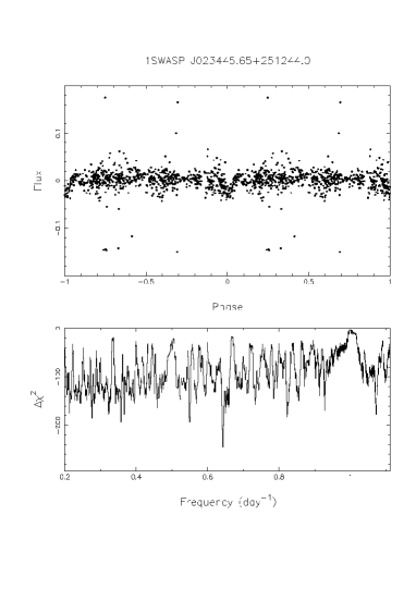
1SWASP J023445.65+251244.0 has a moderate amount of scatter in its light curve, but the transit is well pronounced (Figures 14). The transit depth and spectral types result in similar sized planets of 1.2RJ. The expected transit duration is near the higher end for acceptable values ( 1.2), and further observations are needed to secure this source as ESP and possible very-hot-Jupiter.
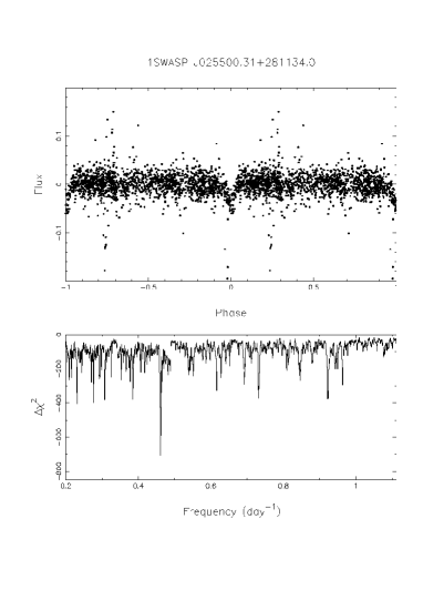
1SWASP J025500.31+281134.0 shows a moderate amount of scatter in its light curve (Figure 15), but does have a well defined period (2.2 days) and transit (3.7%). This transit depth is one of the larger for ESP candidates and results in a planet radius of 1.3 RJ for a spectral type of K0. The slight ’V’ shape to the transit profile and large value of the expected transit duration ( = 1.3) may indicate this is a stellar system.
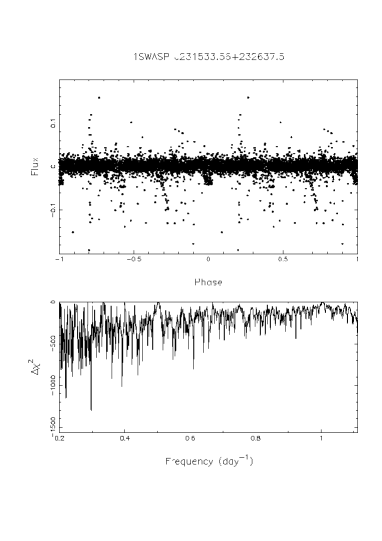
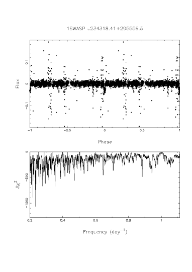
1SWASP J231533.56+232637.5 and 1SWASP J234318.41+295556.5 have a moderate amount of scatter in their light curves, but the transits are well pronounced for both systems (Figures 16 & 17). Their transit depths and spectral types result in similar sized planets of 1.1 and 1.4 RJ, respectively. 1SWASP J234318.41+295556.5 has an ellipsoidal amplitude of 2.9, and may be a stellar binary.
5 Discussion
The majority of candidates found with low amplitude periodic variability showed obvious signatures of being stellar binaries. We have selected only 12 as new ESP candidates. There are many different types of stellar systems and chance alignments that can show behavior mimicking a planet’s transit. Such possibilities have been separated into 3 groups (see for example Brown 2003): 1) grazing incidence stellar binary systems, 2) stellar systems consisting of both a high mass and low mass stars, and 3) an eclipsing stellar system in which some light from a foreground or background star contaminates the light from the binary reducing the depth of the eclipse and making it appear more ’transit-like’. We have scrutinized our sample of low amplitude variables with the techniques outlined in § 3.2, and attempted to eliminate systems from above categories 1 and 2. However, previous studies on ESPs have shown that it is difficult to remove the 3rd category of false-positive transiting system, the diluted stellar binary (Torres et al., 2005; O’Donovan et al., 2006). For this reason, high resolution optical spectroscopy is needed to measure radial velocities for our candidates and determine the companion’s mass. Such follow-up have been successful in identifying 6 such sources from OGLE sample (Konacki et al., 2003, 2004; Bouchy et al., 2004; Pont et al., 2004; Konacki et al., 2005), and is being undertaken by our consortium.
5.1 Expected Numbers of ESP
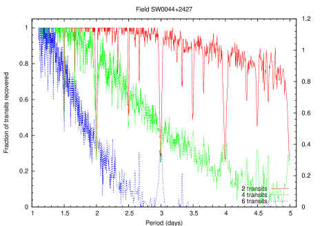
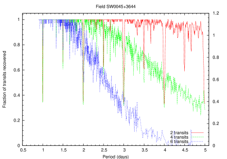
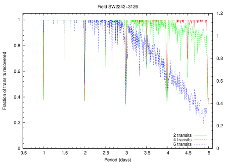
For our sample of 900,000 stars we are left with 400,000 that are brighter than V=13.5 and for which SuperWASP is statistically sensitive to detect a transiting ESP. If we conservatively estimate only 50% of these stars are late-type (F–M) dwarfs, this reduces our sample size to 200,000 stars. If 1% of these have hot-Jupiter companions (Lineweaver & Grether, 2003), and we expect 10% of these to show transits (Horne, 2003), we therefore should have detected 200 ESPs, although this estimate is affected by the true coverage for a particular field. For this reason we have also estimated the expected fraction of transits recovered for each observed field as a function of transit period and for different numbers of transits. These expected transit yields are shown in Figure 18a-c for the recovery of 2, 4, and 6 transits. For sources with periods 5 days and for fields that were observed for 80 or more nights, 2 transits would have been detected 95% of the time. For the fields with poorest coverage the recovered fraction only drops to 80%. However, if we require the recovery of 4 transits, the recovered fraction is reduced to 40% for fields that were observed for at least 80 nights, and 10–20% for fields with 60 nights of coverage. The majority of the fields presented here were observed for at least 60 nights, and hence we should recover 2 transits for 80% of the planets present, leading to an expectation of 160 ESPs detected. If we require the recovery of 4 transits, then this number is reduced to 80.
The plethora of short-period extra-solar planets that was predicted in the mid-1990s and recently (Horne, 2003) has not come to fruition. Surveys that concentrate on wide fields and brighter stars have only 2 transit ESP discoveries (TrES-1, Alonso et al. 2004, and XO-1b, McCullough et al. 2006). The majority of other transiting ESPs (6) have come from the OGLE micro-lensing survey of the Galactic Centre and fields nearby (Udalski et al., 2004 and references therein). Brown (2003) estimated the detection rate for giant ESP including the probability both of a star having a planet and of observing it. This provides an estimate of 1 ESP per 25,000 stars. Photometric surveys of open clusters (OCs) with 2 to 4 metre class telescopes that observe to much fainter magnitudes [e.g. Street et al. (2003); EXPLORE, van Braun et al. (2005); PISCES, Mochejska et al. (2005, 2006)] have also failed to detect short-period ESPs. These surveys have monitored tens of thousands of stars for tens of days with high precision and to very faint magnitudes (R 20), yet found few to no ESPs.
A trend has been established where ESP are found predominately with metal-rich host stars (Fischer & Valenti, 2005; Santos et al., 2003). The lack of ESP transit candidate detections in metal-poor globular cluster, 47 Tuc (Gilliland et al., 2000; Weldrake et al., 2005), is consistent with this. Given that these deep OC surveys are sensitive to short period ESPs, the lack of detections might imply that the frequency of transiting hot-Jupiters is closer to 1 in 50,000 stars. Our present results of 12 ESP candidates in nearly 400,000 stars are consistent with the current detection rates.
There may be several contributing factors to this lack of detections. The weather can seriously diminish the observing duration and shorten the observing window used in many of the estimated ESP yields. Changes in extinction can be difficult to remove from the observations and cause false variability. Additionally, intrinsic stellar variability, especially in stars of later spectral types, may hide the transit signature. Later type stars will have deeper transit depths and these are more easily recovered for fainter stars. For these reasons, we may then consider if the periodic nature of the transit signal would allow us to recover shallower transit depths or transits from stars fainter than 13th magnitude. Periodic signals are most readily recovered from the transit searching algorithm, but we are ultimately limited by the signal-to-noise and duration of the data. Simulations for the fraction of transits recovered based on each of our field’s observing windows have shown that there are several integer periods where the probability of recovering a transit is greatly reduced because of the lack of coverage (e.g. Figure 18a-c), and there also several periods where the chance for detection is actually increased (see Fig 18a, Ntr = 6 case and P=3 days). In a companion paper, Smith et al. (2006) investigate the affects of the noise properties on transit recovery in the SuperWASP data and conclude the best way to reduce the co-variant noise is to increase the observing baseline.
Many improvement to the analysis of photometric transit data have been made, and there are additional tests to distinguish stellar systems from true ESPs (e.g. Tingley & Sackett 2005). The ESP detection rate of the WASP project is presently unknown, but continued SW-N and SW-S observations will discover more high quality ESP candidates. However, it is important to have spectroscopic follow-up to determine the mass function of these systems. It may be left to space-borne missions, such as Kepler and COROT, without the hindrance of the atmosphere, to truly determine the frequency of hot-Jupiter and even Earth-size ESPs.
| Name | S | Period | duration | Epochb | Ntrans | (S/N) | ||
|---|---|---|---|---|---|---|---|---|
| 1SWASP | (days) | (percent) | (hrs) | |||||
| J230808.34+333803.9 | 21.2 | 2.23 | 2.15 | 2.45 | 3149.2152 | 15 | 1922 | 7.3 |
| J231240.14+321540.4 | 12.6 | 2.53 | 3.08 | 2.59 | 3148.7063 | 9 | 969 | 2.10 |
| J231302.08+262724.3 | 11.1 | 4.39 | 2.16 | 3.05 | 3149.1804 | 7 | 1188 | 4.0 |
| J231533.56+232637.5 | 11.6 | 3.36 | 2.89 | 3.79 | 3148.7560 | 10 | 1597 | 0.7 |
| J231807.73+240522.1 | 21.3 | 2.54 | 5.96 | 1.90 | 3150.5115 | 8 | 1281 | 1.5 |
| J232639.10+233219.2 | 16.8 | 2.21 | 3.67 | 2.54 | 3150.3117 | 15 | 3405 | 2.3 |
| J232700.56+200609.1 | 22.3 | 3.24 | 5.79 | 2.45 | 3149.3855 | 11 | 733 | 3.2 |
| J233325.17+332632.1 | 12.4 | 2.27 | 1.59 | 3.34 | 3150.2111 | 16 | 1072 | 9.2 |
| J234318.41+295556.5 | 14.4 | 4.24 | 2.81 | 2.42 | 3151.8626 | 6 | 1213 | 2.9 |
| J000029.25+323300.9 | 14.0 | 1.20 | 2.49 | 2.35 | 3151.9736 | 17 | 939 | 7.2 |
| J000233.27+331516.8 | 15.6 | 2.37 | 3.01 | 2.04 | 3152.5501 | 11 | 1476 | 10.2 |
| J002040.07+315923.7 | 11.6 | 2.52 | 1.27 | 3.00 | 3151.4864 | 9 | 287 | 0.4 |
| J002728.02+284649.2 | 9.7 | 1.52 | 1.22 | 3.17 | 3166.9666 | 12 | 1136 | 2.5 |
| J002819.22+335122.1 | 12.0 | 3.45 | 8.07 | 3.82 | 3165.2148 | 6 | 1033 | 2.6 |
| J003039.21+205719.1 | 10.5 | 2.28 | 1.91 | 2.38 | 3166.6460 | 9 | 668 | 0.4 |
| J004804.21+202258.8 | 25.2 | 1.83 | 6.45 | 2.71 | 3167.0060 | 9 | 3326 | 6.6 |
| J005107.84+214352.7 | 13.7 | 1.47 | 4.24 | 2.42 | 3167.6596 | 8 | 3322 | 5.9 |
| J005225.90+203451.2 | 12.4 | 1.72 | 2.78 | 1.66 | 3166.9509 | 8 | 1198 | 3.7 |
| J005250.45+221038.8 | 19.7 | 2.46 | 6.46 | 2.30 | 3167.0449 | 6 | 1011 | 1.6 |
| J005818.26+204348.0 | 10.8 | 2.20 | 8.83 | 2.54 | 3167.1818 | 7 | 2962 | 7.0 |
| J010151.11+314254.7 | 9.6 | 2.19 | 1.66 | 2.64 | 3167.4457 | 10 | 694 | 3.2 |
| J010553.38+241358.3 | 8.9 | 3.35 | 2.88 | 1.73 | 3165.6700 | 4 | 305 | 1.7 |
| J010706.32+313918.0 | 20.2 | 4.10 | 4.54 | 2.14 | 3167.5442 | 4 | 2569 | 0.2 |
| J013033.21+311447.0 | 7.0 | 4.40 | 1.56 | 3.58 | 3179.5786 | 3 | 408 | 2.3 |
| J013100.45+374745.2 | 15.6 | 1.65 | 3.60 | 2.14 | 3181.5542 | 12 | 841 | 0.1 |
| J013250.08+194332.7 | 10.7 | 3.13 | 5.60 | 4.27 | 3166.2451 | 6 | 1248 | 2.8 |
| J013452.76+293626.5 | 11.8 | 1.91 | 1.53 | 3.31 | 3166.0957 | 14 | 1674 | 1.1 |
| J014400.22+344449.2 | 11.9 | 3.72 | 2.73 | 3.17 | 3180.2839 | 5 | 914 | 4.4 |
| J015625.53+291432.5 | 12.2 | 1.45 | 1.24 | 3.22 | 3182.5415 | 13 | 1084 | 4.9 |
| J015711.29+303447.7 | 12.3 | 2.04 | 1.55 | 2.30 | 3182.5612 | 9 | 1253 | 1.3 |
| J015951.59+354455.4 | 8.5 | 1.19 | 2.28 | 1.97 | 3181.9274 | 13 | 586 | 12.9 |
| J020720.96+325526.5 | 10.1 | 1.54 | 4.52 | 3.22 | 3181.7719 | 10 | 1354 | 5.8 |
| J021217.50+335319.2 | 20.0 | 3.91 | 6.85 | 2.64 | 3180.5364 | 3 | 1883 | 1.0 |
| J022421.03+375419.9 | 11.3 | 4.16 | 5.47 | 2.81 | 3191.8221 | 4 | 2530 | 3.3 |
| J022651.05+373301.7 | 9.6 | 1.22 | 1.29 | 2.02 | 3194.6500 | 8 | 1782 | 4.3 |
| J023445.65+251244.0 | 7.6 | 1.55 | 2.36 | 2.62 | 3194.4315 | 6 | 286 | 1.1 |
| J024206.53+364029.7 | 16.4 | 2.59 | 4.78 | 2.81 | 3193.8696 | 7 | 763 | 3.4 |
| J025419.14+324240.7 | 20.4 | 2.91 | 5.11 | 2.71 | 3192.4337 | 4 | 319 | 0.4 |
| J025500.31+281134.0 | 9.0 | 2.17 | 3.74 | 2.76 | 3191.9254 | 6 | 767 | 1.4 |
| J025712.69+403140.0 | 9.8 | 2.22 | 1.80 | 2.50 | 3192.7651 | 6 | 549 | 10.7 |
| J025958.91+294434.6 | 10.0 | 1.73 | 5.41 | 2.33 | 3193.1976 | 6 | 1010 | 2.3 |
a Sred – Signal-to-red noise (see text).
b JD = 2450005.5 + Epoch
c (S/N)ellip – Amplitude of ellipsoidal variations (see text).
6 Conclusions
We have presented 41 low amplitude variables from the SW-N 2004 observing season. From this list we identified 12 ESPs candidates with periods of 1.2 to 4.4 days. These have transit depths 1–4% implying planetary radii of 1.0–1.5 RJ for their derived spectral types. High resolution optical spectroscopy to measure radial velocities and obtain orbital solutions and masses for these systems are needed to confirm these candidates are true extrasolar planets. Such observations are being undertaken by our consortium. SW-N and SW-S both continue to operate for the 2006 observing season, and with a full 8 cameras complement, and are expected to obtain more than twice the amount of data as the 2004 campaign.
| Name | VSW | VK | JK | Teff | Spec. Type | R⋆ | Rp | Comment | |
|---|---|---|---|---|---|---|---|---|---|
| 1SWASP | R☉ | RJ | |||||||
| J230808.34+333803.9 | 10.8 | 1.41 | 0.28 | 6051 | F9 | 1.14 | 1.43 | 0.85 | Ellip. large |
| J231240.14+321540.4 | 11.8 | 1.46 | 0.30 | 5990 | G0 | 1.11 | 1.66 | 0.85 | Rp too large |
| J231302.08+262724.3 | 10.6 | 3.68 | 0.87 | 4170 | M0 | 0.63 | 0.79 | 1.19 | Giant? |
| J231533.56+232637.5 | 11.6 | 1.72 | 0.35 | 5661 | G6 | 0.96 | 1.39 | 0.13 | ESPc |
| J231807.73+240522.1 | 12.0 | 2.31 | 0.54 | 5034 | K3 | 0.76 | 1.63 | 0.74 | Rp too large |
| J232639.10+233219.2 | 11.5 | 1.26 | 0.22 | 6256 | F7 | 1.25 | 2.04 | 0.81 | Rp too large |
| J232700.56+200609.1 | 12.5 | 1.55 | 0.29 | 5870 | G2 | 1.05 | 2.16 | 0.73 | Rp too large |
| J233325.17+332632.1 | 11.1 | 1.74 | 0.41 | 5637 | G6 | 0.95 | 1.01 | 1.25 | Ellip. large |
| J234318.41+295556.5 | 10.7 | 2.31 | 0.55 | 5034 | K3 | 0.76 | 1.09 | 0.84 | ESPc |
| J000029.25+323300.9 | 12.0 | 2.24 | 0.57 | 5101 | K2 | 0.77 | 1.01 | 1.29 | Ellip. large |
| J000233.27+331516.8 | 11.3 | 1.04 | 0.29 | 6573 | F4 | 1.40 | 2.07 | 0.60 | Rp too large |
| J002040.07+315923.7 | 11.8 | 1.51 | 0.31 | 5921 | G1 | 1.08 | 1.04 | 1.06 | ESPc |
| J002728.02+284649.2 | 9.6 | 2.84 | 0.71 | 4602 | K5 | 0.69 | 0.65 | 1.72 | Giant?/Large |
| J002819.22+335122.1 | 12.5 | 1.52 | 0.35 | 5908 | G1 | 1.07 | 2.39 | 0.98 | Rp too large |
| J003039.21+205719.1 | 11.0 | 1.31 | 0.55 | 6186 | F8 | 1.21 | 1.23 | 0.92 | ESPc |
| J004804.21+202258.8 | 10.7 | 2.08 | 0.50 | 5260 | K1 | 0.82 | 1.78 | 1.1 | Ellip. large |
| J005107.84+214352.7 | 11.1 | 1.51 | 0.30 | 5921 | G1 | 1.08 | 1.90 | 0.95 | Rp too large |
| J005225.90+203451.2 | 11.2 | 1.89 | 0.46 | 5465 | G9 | 0.88 | 1.25 | 0.71 | ESPc |
| J005250.45+221038.8 | 12.3 | 1.47 | 0.33 | 5973 | G0 | 1.10 | 2.38 | 0.74 | Rp too large |
| J005818.26+204348.0 | 12.4 | 1.77 | 0.38 | 5602 | G7 | 0.93 | 2.09 | 0.63 | Rp too large |
| J010151.11+314254.7 | 11.1 | 1.04 | 0.17 | 6573 | F4 | 1.40 | 1.42 | 1.04 | ESPc |
| J010553.38+241358.3 | 11.1 | 1.49 | 0.33 | 5947 | G1 | 1.09 | 1.58 | 0.53 | Rp large |
| J010706.32+313918.0 | 10.3 | 1.55 | 0.30 | 5870 | G2 | 1.05 | 1.91 | 0.6 | Rp too large |
| J013033.21+311447.0 | 10.6 | 1.64 | 0.34 | 5758 | G4 | 1.00 | 1.07 | 1.08 | ESPc |
| J013100.45+374745.2 | 11.1 | 1.35 | 0.30 | 6130 | F8 | 1.18 | 1.90 | 0.78 | Rp large |
| J013250.08+194332.7 | 11.4 | 1.91 | 0.42 | 5442 | G9 | 0.87 | 1.76 | 0.14 | Rp too large |
| J013452.76+293626.5 | 10.1 | 2.68 | 0.64 | 4720 | K5 | 0.70 | 0.40 | 1.60 | Giant/Large |
| J014400.22+344449.2 | 11.2 | 1.30 | 0.25 | 6200 | F8 | 1.22 | 1.72 | 0.88 | Rp too large |
| J015625.53+291432.5 | 10.3 | 2.30 | 0.54 | 5044 | K3 | 0.76 | 0.72 | 1.67 | ESPc?/Large |
| J015711.29+303447.7 | 10.4 | 1.19 | 0.34 | 6354 | F6 | 1.30 | 1.38 | 0.77 | ESPc |
| J015951.59+354455.4 | 11.0 | 3.07 | 0.73 | 4453 | K7 | 0.67 | 0.86 | 0.08 | Ellip. large |
| J020720.96+325526.5 | 12.4 | 2.27 | 0.65 | 5072 | K2 | 0.77 | 1.40 | 1.51 | Ellip. large |
| J021217.50+335319.2 | 11.2 | 2.62 | 0.67 | 4767 | K5 | 0.71 | 1.59 | 0.92 | Rp large |
| J022421.03+375419.9 | 10.7 | 1.70 | 0.30 | 5685 | G5 | 0.97 | 1.94 | 0.81 | Rp too large |
| J022651.05+373301.7 | 8.3 | 0.83 | 0.11 | 6896 | F1 | 1.52 | 1.47 | 0.74 | ESPc |
| J023445.65+251244.0 | 12.1 | 1.86 | 0.35 | 5498 | G8 | 0.89 | 1.17 | 1.17 | ESPc |
| J024206.53+364029.7 | 11.8 | 1.47 | 0.29 | 5973 | G0 | 1.10 | 2.05 | 0.89 | Rp too large |
| J025419.14+324240.7 | 11.7 | 1.61 | 0.37 | 5795 | G3 | 1.02 | 1.97 | 0.86 | Rp too large |
| J025500.31+281134.0 | 11.8 | 2.00 | 0.45 | 5344 | K0 | 0.84 | 1.34 | 1.29 | ESPc |
| J025712.69+403140.0 | 10.6 | 1.13 | 0.17 | 6441 | F6 | 1.34 | 1.53 | 0.80 | Ellip. large |
| J025958.91+294434.6 | 12.2 | 1.57 | 0.21 | 5845 | G2 | 1.04 | 2.11 | 0.71 | Rp too large |
Acknowledgments
The WASP consortium consists of representatives from the Queen’s University Belfast, University of Cambridge (Wide Field Astronomy Unit), Instituto de Astrofísica de Canarias, Isaac Newton Group of Telescopes (La Palma), University of Keele, University of Leicester, The Open University, and the University of St Andrews. The SuperWASP-N and SuperWASP-S instruments were constructed and operated with funds made available from Consortium Universities and the Particle Physics and Astronomy Research Council. SuperWASP North is located in the Spanish Roque de Los Muchachos Observatory on La Palma, Canary Islands which is operated by the Instituto de Astrofísica de Canarias (IAC). We thank an anonymous referee for suggested improvements, and acknowledge useful scientific discussion with I. Dino, J. Smoker, and C. Snodgrass. We are grateful to PPARC for financial support.
References
- Aigrain & Favata (2002) Aigrain, S. & Favata, F. 2002, A&A, 395, 625
- Alonso et al. (2004) Alonso, R. et al. 2004, ApJ, 613, L153
- Ammons et al. (2006) Ammons, S.M., Robinson, S.E., Strader, J., Laughlin, G., Fischer, D., Wolf, A. 2006, ApJ, 638, 1004
- Bouchy et al. (2004) Bouchy, F. et al. 2004, A&A, 421, L13
- Bouchy et al. (2005) Bouchy, F., Pont, F., Melo, C., Santos, N. C., Mayor, M., Queloz, D., Udry, S. et al. 2005a, A&A, 431, 1105
- Bouchy et al. (2005) Bouchy, F. et al. 2005b, A&A, 444, L15
- Brown (2003) Brown, T. 2003, ApJ, 593, L125
- Burke et al. (2006) Burke, C.J., Gaudi, B.S., Depow, D.L., & Pogge, R.W. 2006, ApJ, in press and astroph/0512207
- Butler et al. (2006) Butler, R.P. et al. 2006, ApJ, 646, 505
- Charbonneau et al. (2000) Charbonneau, D., Brown, T. M., Latham, D. W., & Mayor, M. 2000, ApJ, 529, L45
- Christian et al. (2005) Christian, D.J. et al. 2005, 13th Cambridge Workshop on Cool Stars, Stellar Systems and the Sun, eds. F. Favata, A.J. Hussain, & B. Battrick, ESA SP-560, 475
- Collier-Cameron et al. (2006) Collier-Cameron, A. et al. 2006, MNRAS, submitted
- Defaÿ et al. (2001) Defaÿ, C., Deleuil, M., & Barge, P. 2001, A&A, 365, 330
- Enoch et al. (2006) Enoch, B. et al. 2006, in prep.
- Fischer & Valenti (2005) Fischer, D.A., Valenti, J. 2005, ApJ, 622, 1102
- Gilliland et al. (2000) Gilliland, R. et al. 2000, ApJ, 545, L47
- Gray (1992) Gray, D.F. The observation and analysis of stellar photospheres 1992, Cambridge University Press
- Henry et al. (2000) Henry, G.W., Margy, G.W., Butler, R.P., & Vogt, S.S. 2000 ApJ, 529, L41
- Horne (2003) Horne, K. 2003, in ASP Conference Series vol. 294, Scientific Frontiers in Research on Extrasolar Planets, eds. D. Deming & S. Seager (San Francisco: ASP), 361
- Jayawardhana et al. (1998) Jayawardhana, R. et al. 1998, ApJ, 503, 79
- Kane et al. (2004) Kane, S.R. et al. 2004, MNRAS, 353, 689
- Kane et al. (2005) Kane, S.R. et al. 2005, MNRAS, 364, 1091
- Kay (1998) Kay, S. 1998, Fundamentals of Statistical Signal Processing: Detection Theory (Upper Saddle River: Prentice-Hall PTR)
- Konacki et al. (2003) Konacki M., Torres G., Jha S., Sasselov D. 2003, Nature, 421, 507
- Konacki et al. (2004) Konacki, M. et al. 2004, ApJ, 609, L37
- Konacki et al. (2005) Konacki, M., Torres, G., Sasselov, D.D., Jha, S. 2005, ApJ, 624, 372
- Kovács et al. (2002) Kovács, G., Zucker, S., Mazeh, T. 2002, A&A, 391, 369
- Lecavelier Des Etangs et al. (1997) Lecavelier Des Etangs, A. et al. 1997, A&A, 325, 228
- Lineweaver & Grether (2003) Lineweaver, C.H., & Grether, D. 2003, ApJ, 598,1350
- Marcy & Butler (1998) Marcy, G.W. & Butler, R.P. 1998, ARA&A, 36, 57
- Marcy & Butler (2000) Marcy, G. & Butler, R. P. 2000, PASP, 112, 137
- Mayor & Queloz (1995) Mayor, M. & Queloz, D. 1995, Nature, 378, 355
- McCullough et al. (2006) McCullough et al. 2006, ApJ, in pres (astro-ph/060541v1)
- Mochejska et al. (2005) Mochejska, B. J et al. 2005, AJ, 129, 2856
- Mochejska et al. (2006) Mochejska, B. J et al. 2006, AJ, 131, 1090
- Moutou et al. (2005) Moutou, C. et al. 2005, A&A, 437, 355
- O’Donovan et al. (2006) O’Donovan, F.T et al. 2006, astroph/200603005
- Pollacco et al. (2006) Pollacco, D.L. et al. 2006, PASP, submitted
- Pont et al. (2004) Pont, F., Bouchy, F., Queloz, D., Santos, N.C., Melo, C., Mayor, M., Udry, S. 2004 A&A, 426, L15
- Robin et al. (2003 and references therein) Robin, A.C., Reylé, C., Derriére, S., & Picaud, S. 2003, A&A, 409, 523
- Santos et al. (2003) Santos, N.C., Israelian, G., Mayor, M., Udry, S. 2003, A&A, 398, 363
- Sirko & Paczyński (2003) Sirko, E., & Paczyński, B. 2003, ApJ, 592, 1217
- Smith & Terrile (1984) Smith, B. A. & Terrile, R. J., Sci, 226, 1421
- Smith et al. (2006) Smith, M.S., Collier Cameron, A, Christian, D.J. et al. 2006, MNRAS, submitted
- Street et al. (2003) Street, R.A. et al. 2003, MNRAS, 340, 1287
- Tamuz et al. (2005) Tamuz, O., Mazeh, T., Zuckerm S. 2005, MNRAS, 356, 1466
- Tingley et al. (2003) Tingley, B. 2003, A&A, 403, 329
- Tingley & Sackett (2005) Tingley, B., & Sackett, P.D. 2005, ApJ, 627, 1011
- Tyson & Gal (1993) Tyson, N.D. & Gal, R. 1993, AJ, 105, 1206
- Torres et al. (2005) Torres, G., Konacki, M., Sasselov, D.D., & Jha, S. 2005, ApJ, 619, 558
- Udry et al. (2000) Udry, S. et al. 2000, A&A, 356, 590
- Udalski et al. (2004 and references therein) Udalski et al. 2004, Acta Astron., 54, 313
- van Braun et al. (2005) von Braun, K., Lee, B.L., Seager, S., Yee, H.K.C., Mallén-Ornelas, G., Gladders, M.D. 2005, PASP, 117, 141
- Weldrake et al. (2005) Weldrake, D.T.F., Sackett, P.D., Bridges, T.J., Freeman, K.C. 2005, ApJ, 620, 1043
- Wilson et al. (2006) Wilson, D.M. et al. 2006, PASP, in press (astroph/0607591)