Status of IceCube in 2005

Abstract

IceCube is a kilometer scale neutrino observatory now in construction at the South Pole. The construction started in January 2005 with the deployment of 76 sensors on the first string and four surface detector stations. Nine strings and 32 surface detectors are in operation since February 2006. The data based on calibration measurements, muons and artificial light flashes are consistent with performance expectations. This report focuses on design, construction experience and first data from the sensors deployed in January 2005.

1 Introduction

The IceCube neutrino observatory is a kilometer scale neutrino telescope currently in construction at the South Pole. The feasibility of a neutrino telescope in ice has been demonstrated by the successful installation and operation of AMANDA. The current AMANDA array will be surrounded by the IceCube array. IceCube is designed to detect astrophysical neutrino fluxes at energies from a few 100 GeV up to highest energies of $10^{9}$ GeV [1], [2]. This report provides an outline of the current construction status, first experiences with construction and first results and conclusions from data obtained from sensors now in the ice.

2 Design of instrument

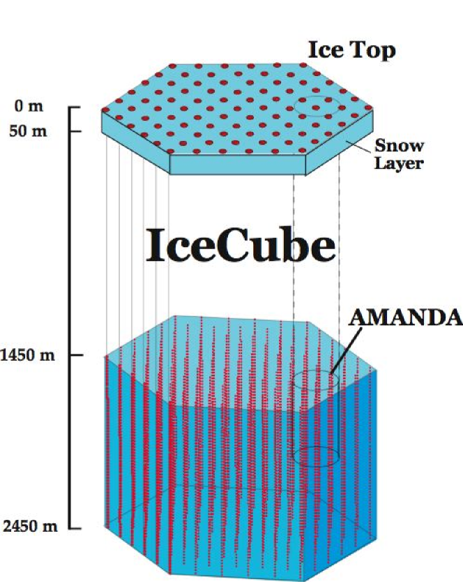
Figure 1: Schematic view of the IceCube array consisting of 80 strings with 60 sensors on each string. The surface detector IceTop consists of 160 tanks, of which two are associated with each string.

The IceCube neutrino observatory at the South Pole will consist of 4800 optical sensors - digital optical modules (DOMs), installed on 80 strings between the depths of 1450 m and 2450 m in the Antarctic Ice, and 320 sensors deployed in 160 IceTop tanks on the ice surface in pairs directly above the strings. Each sensor consists of a photomultiplier tube, connected to a waveform-recording data acquisition circuit capable of resolving pulses with nanosecond precision and having a dynamic range of at least 250 photoelectrons per 10 ns. A total of 76 sensors were installed in January 2005, 60 on the first IceCube string and 16 in the first 8 IceTop tanks. The table summarizes the construction status as of February 2006.

Year	Strings	Tanks	Sensors
Deployed in 2004/05	1	8	76
Deployed in 2005/06	8	24	528
Configuration in 2006	9	32	604

Following the AMANDA concept, it was a design goal to avoid single point failures in the ice, which is not accessible once frozen. 30 twisted pair copper cables packaged in 15 twisted quads are used to provide power and communication to 60 sensors. A string consists of the following major configuration items: a cable from the counting house to the string location, a cable from the surface to 2450 m depth, and 60 optical sensors. The main cable is about 2500 m long and 42 mm in diameter with a weight of 6 t. Three additional quads provide communication to pressure sensors and local communication between optical sensors. Every 17 m there is a mounting structure (Yalegrip) to allow a quick mechanical attachment of the sensors. To reduce the amount of cable, two sensors are operated on the same wire pair, one terminated and one unterminated. Neighboring sensors are connected to enable fast local coincidence triggering in the ice. Each sensor has a direct connection to the data acquisition computers in the central counting house.

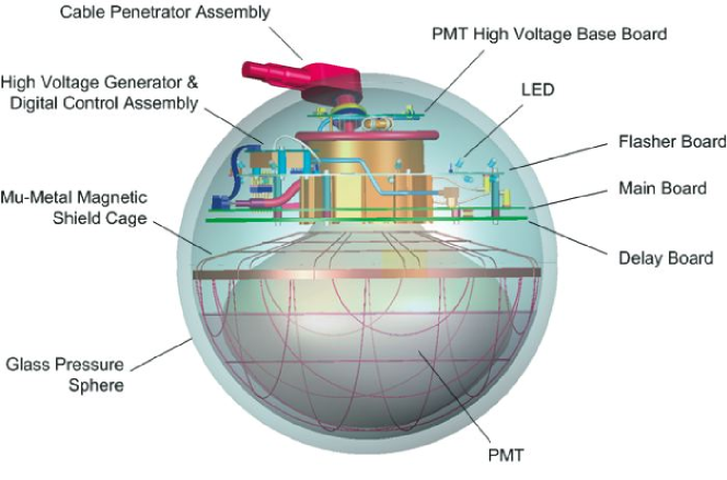
Figure 2: Schematic view of a Digital Optical Module.

A schematic view of an optical sensor is shown in Fig. 2. An optical sensor consists of a 25 cm diameter photomultiplier tube (PMT) embedded in a glass pressure vessel of 32.5 cm diameter. The HAMAMATSU R7081-02 PMT has ten dynodes allowing operation at a gain of at least $5\cdot 10^{7}$. The typical gain in operation is $0.5-1.0\cdot 10^{7}$ providing a single photoelectron amplitude of about 10 mV. The PMT signal is amplified by 3 different gains (x0.25, x2, x16) to extend the dynamic range. The signals are digitized by a fast analog transient waveform recorder (ATWD) and by a flash ADC (40 MHz). The ATWD uses a 128 sample switched capacitor array which is operated at a sampling rate of 3.3 ns/sample. The linear dynamic range of the sensor is 400 photoelectrons in 15 ns and the integrated dynamic range is of more than 5,000 photoelectrons in 2 $\mu$s. The PMT analog pulse is delayed by 75 ns on a separate circuit board to account for the time needed to make the trigger decision and initiate the ATWD for readout. The digital electronics on the main board are based on a 400k-gate field programmable gate array (FPGA) which contains a 32-bit CPU, 8 MB of flash storage, and 32 MB of RAM. A small communications program stored in ROM allows communication to be established with the surface computer system and then to download updated software.

The flasher board is an optical beacon integrated in each DOM. It contains a total of 12 LEDs; 6 pointing horizontally and 6 pointing 48 degrees upward. The LEDs can be fired individually or as a group and the amplitude can be adjusted over a wide range up to a brightness of $10^{10}$ photons/pulse at a wavelength of about 410 nm. The flasherboard allows for a variety of calibration functions, for example timing and geometry verification.

The high voltage is generated by an HV generator, which is located on a separate board. The base is a simple resistor chain with appropriate capacitors. All electronics of the DOM were designed for high reliability and stress testing was performed to screen for high quality. Low power consumption was a design goal, the power of a single DOM being 3 W in normal operation.

3 Data acquisition and online data processing

All photomultiplier pulses are to be sent to the surface, but a local coincidence (LC) trigger scheme is used to apply data compression for isolated hits. Isolated hits are mostly noise pulses. For the LC trigger they are defined as pulses for which no signal was recorded in the neighboring sensors within $\approx\pm 800$ ns. All other hits are being transmitted with full waveform information. The data acquisition system in 2005 is based on the system that is used for the final acceptance testing of the sensors during and after production. A full data acquisition with increased functionality will be used in 2006.

The detector electronics and software are designed to require minimal maintenance at the remote location. For example the time calibration system, a critical part of a neutrino telescope, is designed to be a self calibrating, integral part of the readout system (in contrast to the AMANDA detector, which required manual calibration of all analog detector channels.) The strings are calibrated as soon as they are frozen-in allowing for gradual commissioning of the instrument. The collaboration plans to do the first science with the array of 9 strings in 2006.

The full detector will trigger at a rate of about 1.5 kHz from down-going muons. This data set will be reduced by at least an order of magnitude, small enough for transmission by satellite. This is done by an online computer farm, which will filter events, compress the data volume of the muon background and select all potentially interesting events for satellite transmission. A complete copy of the full, unfiltered data set will be written on tape for later access.

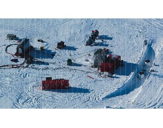
Figure 3: Aerial view of the tower operations site for the first IceCube string 29 in January 2005: Hose reel on left (weight: 40t), drill tower with associated heated drilling and deployment structure on center-right. The excavation for two IceTop Cherenkov tanks is visible on the right.

4 Construction

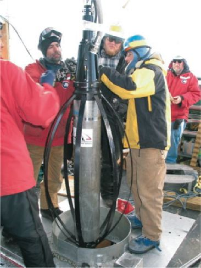
Figure 4: IceCube drillers are rigging the drill moments before it descends to a depth of 2500 m.

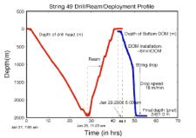
Figure 5: Depth versus time profile for the drillhead during drilling of hole 49. Also shown is the string installation of the bottom end of the string.

The detector is constructed by drilling holes in the ice using a hot-water drill. The first operation of the new enhanced hot water drill (EHWD) in January 2005 was a challenging task. The drill system consists of numerous pump and heating systems, hoses, a drill tower and a complex control system. While drilling the first hole it successfully provided a thermal power of about 5 MW, consistent with the design specification and a factor two more powerful than the drill used for AMANDA. The drill is designed to drill holes to a depth of 2500 m in a period of less than 35 hours, excluding the time needed for rigging. In comparison, the drilling for AMANDA required typically 90 h to reach a depth of 2000 m. Fig. 3 shows the drill tower with several reels during drilling of the first hole. Fig. 4 shows the rigging of the drill head moments before it descends to its 2500 m deep round trip. Fig. 5 shows the depth of the drill head and the string as a function of time for the first hole/string. The completed hole is of $\approx$60 cm diameter and filled with water up to about 50 m below the snow layer. The water filled hole freezes within about a week and it is designed large enough to allow 24 h for the string installation. The string is then deployed into the water-filled hole within less than 12 hours.

This method has been pioneered and developed by AMANDA. IceCube will use this improved drill and deployment equipment to deploy up to 16 strings during a South Pole construction season, which lasts from November to mid-February.

5 Engineering data - first measurements

The collaboration reported first results, which show that the detector system works as expected [3]. All of the 76 sensors were found to communicate and produce excellent data. A variety of data was taken, including cosmic ray muon data, neutrino candidates, light flasher events, coincident muon events with AMANDA and coincident airshower events with IceTop. All of these data produced results consistent with expectations.

Figure 6: The time difference of a flasher pulse is measured between two optical sensors at 17 m and 34 m distance, respectively. The time difference for all sensors constitutes a system level time resolution verification.

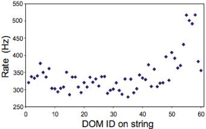
Figure 7: Observed single photoelectron noise rates on the first IceCube string. The DOM ID from 1 to 60 on the string describes the position of the sensor at a depth from 1450 m to 2450 m. The measurement was made with an intentional deadtime of 51 $\mu$s.

An accurate time calibration system is very important for the experiment. All sensors have precise local quartz oscillators. The measurement of the signal transit time through the cable is a prerequisite for the determination of the absolute time of the local clocks. This is done by sending a pulse to the sensor, which is recorded by the DOM and then sent back and recorded again at the surface. Once the cable transit time is known the DOMs can be synchronized to GPS time. The local clocks are synchronized every 5 seconds to the central GPS clock at a precision of less than 3 ns. LED flashers are used to demonstrate relative timing and geometry. Fig. 6 shows the time resolution of sensors as measured with light flashers. The time difference of bright pulses are measured with the two adjacent sensors. The average rms of less than 1.5 ns is proof that the relative timing of sensors is stable.

Another first measurement, which was awaited with much interest was the single photoelectron noise rate of the sensors in situ. We know from AMANDA that the noise rates of photomultipliers in ice are relatively low, of order 1 kHz. There is no known background from the ice other than photons generated by cosmic particles. The noise background is dominated by light generated in the glass of the pressure housing and the glass of the photomultiplier. For IceCube further efforts had been made to reduce the number of photons generated by radioactivity in the sensors, and hence the DOM dark rates. Once the string was frozen and the temperatures approached equilibrium the noise of the sensors settled at a rate of $\approx$700 Hz when measured without after-pulse suppression. The rate is $\approx$350 Hz as shown in Fig. 7 when measured with after-pulse suppression of 51 $\mu$s. The first value is relevant for the data rates. The latter value exceeds earlier expectations. It is important for the sensitivity of IceCube to detect the low energy neutrino pulse associated with supernova explosions. Due to improved glass quality the noise rate of the IceCube sensors is substantially smaller than for AMANDA, while the optical sensitivity is about 1.4 times larger.

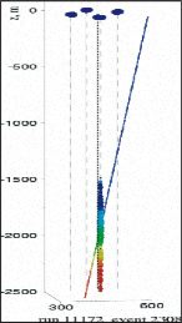
Figure 8: Event display of an air shower detected in the surface detector stations with a coincident muon observed in string 29.

Figure 9: Time delays of measured photons with respect to the nominal muon Cherenkov time. The time residuals are a verification of the timing system and the detector response to muons.

Muon tracks have been used to test the timing of individual sensors. A system level verification of the time resolution of a sensor can be done by comparing the time response of that sensor with the fitted Cherenkov time based on all other sensors on the single string. An example of an event is shown in Fig. 8. The event has been recorded in eight ice Cherenkov detectors at the surface and in most of the sensors on the deep string. In this event detector system records an air shower over a distance of 2500 m. Fig. 9 shows the time delay distribution of a sensor with respect to the nominal Cherenkov cone arrival time. The distribution is centered around zero with some photons delayed due to scattering.

Muon zenith angle distributions taken with the first string showed agreements with simulations. Cosmic ray muons are not only considered as background but used for several purposes in IceCube. While the optical sensors are pointing downward, the sensitivity for downward going muons is approximately as good as for upward going muons. Muons can be used to verify the geometry and and the detector acceptance using the high statistics of downgoing muons. Muons may also be used to verify the IceCube absolute pointing resolution using the cosmic ray shadow of the Moon, as has been done with other surface airshower and with underground detectors. We also plan to do cosmic ray air shower physics using deep ice muon data in coincidence with the surface airshower data taken with the detector system IceTop, which is an important part of the IceCube observatory.

6 Performance of the complete array

Detailed performance studies were performed using MonteCarlo simulations [1], [2]. The reconstruction algorithms used for AMANDA yield an angular resolution of $0.7^{\circ}$ at 10 TeV. The effective area for muons is about 0.8 km² for 1 TeV muons after background rejection and exceeding 1 km² at higher energies. IceCube is expected to trigger at a rate of 1.5 kHz on cosmic ray muons and yield about $10^{5}$ atmospheric neutrinos per year. The effective area for muons after background rejection  is shown in Fig. 10 [1]. The combined underground and surface detector will allow the measurement of air shower parameters in detail beyond energies of $10^{9}$GeV. During the construction phase until 2010 IceCube will grow year be year in size and performance providing a steady inrease in sensitivity.

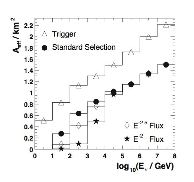
Figure 10: The effective area of IceCube for muons is shown versus muon energy.

7 Conclusions

The successful deployment of the first IceCube string in January 2005 provided the basis for confidence in the detector design and the overall construction schedule. The IceCube collaboration was able to extract data from the first 76 sensors that show that the detector works. Noise rates, timing calibrations and muon distributions are consistent with expectations. Eight more strings were deployed in the 2005/06 season. IceCube is already now, with 9 strings and 16 IceTop stations, the largest neutrino detector taking data in the world with a total of 604 optical sensors deployed. Moreover it can be jointly operated with the existing 677 optical sensor AMANDA-II array. The combined detector has started taking science quality data in 2006.

8 Acknoweldgements

This research was supported by the Deutsche Forschungsgemeinschaft (DFG); German Ministry for Education and Research; Knut and Alice Wallenberg Foundation, Sweden; Swedish Research Council; Swedish Natural Science Research Council; Fund for Scientific Research (FNRS-FWO), Flanders Institute (IWT), Belgian Federal Office for Scientific, Technical and Cultural affairs (OSTC), Belgium. UC-Irvine AENEAS Supercomputer Facility; University of Wisconsin Alumni Research Foundation; U.S. National Science Foundation, Office of Polar Programs; U.S. National Science Foundation, Physics Division; U.S. Department of Energy.

References

- [1] J. Ahrens et al., Astrop. Phys. 20, 507 (2004), arXiv:astro-ph/0305196.
- [2] IceCube Project Preliminary Design Document, Ahrens et al. (IceCube collaboration) http://icecube.wisc.edu
- [3] The IceCube Collaboration: Proc. to the 29th ICRC 2005, Pune, India, Aug. 2005; astro-ph/0509330