Performance Analysis of Direct $N$-Body Algorithms on Special-Purpose Supercomputers

Abstract

Direct-summation $N$-body algorithms compute the gravitational interaction between stars in an exact way and have a computational complexity of $\mathcal{O}(N^{2})$. Performance can be greatly enhanced via the use of special-purpose accelerator boards like the GRAPE-6A. However the memory of the GRAPE boards is limited. Here, we present a performance analysis of direct $N$-body codes on two parallel supercomputers that incorporate special-purpose boards, allowing as many as four million particles to be integrated. Both computers employ high-speed, Infiniband interconnects to minimize communication overhead, which can otherwise become significant due to the small number of “active” particles at each time step. We find that the computation time scales well with processor number; for $2\times 10^{6}$ particles, efficiencies greater than 50% and speeds in excess of $2\,\mathrm{TFlops}$ are reached.

, , , , ,

1 Introduction

Numerical algorithms for solving the gravitational $N$-body problem (Aarseth 2003) have evolved along two basic lines in recent years. Direct-summation codes compute the complete set of $N^{2}$ interparticle forces at each time step; these codes are designed for systems in which the finite-$N$ graininess of the potential is important or in which binary- or multiple-star systems form, and until recently, were limited by their $\mathcal{O}(N^{2})$ scaling to moderate ($N\mathrel{\mathchoice{\lower 3.6pt\vbox{\halign{$\mathsurround=0pt\displaystyle\hfil#\hfil$\cr<\crcr\sim\crcr}}}{\lower 3.6pt\vbox{\halign{$\mathsurround=0pt\textstyle\hfil#\hfil$\cr<\crcr\sim\crcr}}}{\lower 3.6pt\vbox{\halign{$\mathsurround=0pt\scriptstyle\hfil#\hfil$\cr<\crcr\sim\crcr}}}{\lower 3.6pt\vbox{\halign{$\mathsurround=0pt\scriptscriptstyle\hfil#\hfil$\cr<\crcr\sim\crcr}}}}10^{5}$) particle numbers. The best-known examples are the NBODY series of codes introduced by Aarseth (1999) and the Starlab environment developed by McMillan, Hut, and collaborators (e.g. Portegies Zwart et al. (2001)).

A second class of $N$-body algorithms replace the direct summation of forces from distant particles by an approximation scheme. Examples are the Barnes-Hut tree code (Barnes and Hut 1986), which reduces the number of force calculations by subdividing particles into an oct-tree, and fast multipole algorithms which represent the large-scale potential via a truncated basis-set expansion (van Albada and van Gorkom 1977; Greengard and Rokhlin 1987), or on a grid (Miller and Prendergast 1968; Efstathiou and Eastwood 1981). These algorithms have a milder, $\mathcal{O}(N\log N)$ or even $\mathcal{O}(N)$ scaling for the force calculations and can handle much larger particle numbers, although their accuracy can be substantially lower than that of the direct-summation codes (Spurzem 1999). The efficiency of both sorts of algorithm can be considerably increased by the use of individual time steps for advancing particle positions (Aarseth 2003).

The $N$-body problem is particularly challenging in the case of dense stellar systems like galactic nuclei, which may contain single or multiple, supermassive black holes in addition to stars (Ferrarese and Ford 2005; Merritt and Milosavljević 2005). Particle advancement must be very accurate for trajectories that pass near the black hole(s). In addition, galactic nuclei are often “collisional” in the sense that gravitational encounters (i.e. scattering) can redistribute energy between stars on time scales less than the age of the universe (Merritt 2006). Simulating the evolution of a collisional nucleus is probably not feasible using tree or grid algorithms due to their limited accuracies. While alternative, highly-efficient algorithms based on the Fokker-Planck or fluid formalisms have been widely used to model galactic nuclei (Louis and Spurzem 1991; Freitag and Benz 2001), these methods can not deal with systems that are far from dynamical equilibrium or that fail to respect spatial symmetries.

A natural way to increase both the speed and particle number in an $N$-body simulation is to parallelize (Dubinski 1996; Pearce and Couchman 1997). Parallelization on general-purpose supercomputers is difficult, however, because the calculation cost is often dominated by a small number of particles in a single dense region, e.g. the nucleus of a galaxy. Communication latency becomes the bottleneck: the time to communicate particle positions between processors can exceed the time spent computing the forces. The best such schemes use systolic algorithms (in which the particles are rhythmically passed around a ring of processors) coupled with non-blocking communication between the processors to reduce the latency (Makino 2002; Dorband et al. 2003).

A major breakthrough in direct-summation $N$-body simulations came in the late 1990s with the development of the GRAPE series of special-purpose computers (Makino and Taiji 1998), which achieve spectacular speedups by implementing the entire force calculation in hardware and placing many force pipelines on a single chip. The GRAPE-6, in its standard implementation (32 chips, 192 pipelines), can achieve sustained speeds of about 1 Tflops at a cost of just $\sim\$50$K. In a standard setup, the GRAPE-6 is attached to a single host workstation, in much the same way that a floating-point or graphics accelerator card is used. Advancement of particle positions [$\mathcal{O}(N)$] is carried out on the host computer, while interparticle forces [$\mathcal{O}(N^{2})$] are computed on the GRAPE. More recently, “mini-GRAPEs” (GRAPE-6A) (Fukushige et al. 2005) have become available, which are designed to be incorporated into the nodes of a parallel computer. The mini-GRAPEs place four processor chips on a single PCI card and delivering a theoretical peak performance of $\sim 131$ Gflops for systems of up to 128k particles, at a cost of $\sim\$6$K. By incorporating mini-GRAPEs into a cluster, both large ($\mathrel{\mathchoice{\lower 3.6pt\vbox{\halign{$\mathsurround=0pt\displaystyle\hfil#\hfil$\cr>\crcr\sim\crcr}}}{\lower 3.6pt\vbox{\halign{$\mathsurround=0pt\textstyle\hfil#\hfil$\cr>\crcr\sim\crcr}}}{\lower 3.6pt\vbox{\halign{$\mathsurround=0pt\scriptstyle\hfil#\hfil$\cr>\crcr\sim\crcr}}}{\lower 3.6pt\vbox{\halign{$\mathsurround=0pt\scriptscriptstyle\hfil#\hfil$\cr>\crcr\sim\crcr}}}}10^{6}$) particle numbers and high ($\mathrel{\mathchoice{\lower 3.6pt\vbox{\halign{$\mathsurround=0pt\displaystyle\hfil#\hfil$\cr>\crcr\sim\crcr}}}{\lower 3.6pt\vbox{\halign{$\mathsurround=0pt\textstyle\hfil#\hfil$\cr>\crcr\sim\crcr}}}{\lower 3.6pt\vbox{\halign{$\mathsurround=0pt\scriptstyle\hfil#\hfil$\cr>\crcr\sim\crcr}}}{\lower 3.6pt\vbox{\halign{$\mathsurround=0pt\scriptscriptstyle\hfil#\hfil$\cr>\crcr\sim\crcr}}}}1\,\mathrm{TFlops}$) speeds can in principle be achieved.

In this paper, we describe the performance of direct-summation $N$-body algorithms on two computer clusters that incorporate GRAPE hardware. §2 describes the hardware implementations. The parallel $N$-body code and its implementation on the GRAPEs is described in §3. §4 presents the results of performance tests using realistic galaxy models, and §5 describes a theoretical performance model that reproduces the observed performance and which can be used to predict the performance of similar codes on different clusters. §6 summarizes our results and discusses directions for future work.

2 Hardware

2.1 The GRAPE technology

The GRAPE-6A board (Fig. 1) is a standard PCI short card on which a processor, an interface unit, and a power supply are integrated. The processor is a module consisting of four GRAPE-6 processor chips, eight SSRAM chips and one FPGA chip. The processor chips each contain six force calculation pipelines, a predictor pipeline, a memory interface, a control unit, and I/O ports (Makino et al. 2003). The SSRAM chips store the particle data. The four GRAPE chips can calculate forces, their time derivatives and the scalar gravitational potential simultaneously on a maximum of 48 particles at a time; this limit is set by the number of pipelines (six force calculation pipelines each of which serves as eight virtual multiple pipelines). There is also a facility to calculate neighbor lists from predefined neighbor search radii; this feature is not used in the algorithms presented below. The forces computed by the processor chips are summed in an FPGA chip and sent to the host computer. A maximum of 131 072 ($2^{17}$) particles can be stored in the GRAPE-6A memory. The peak speed of the GRAPE-6A is 131.3$\,\mathrm{GFlops}$ (when computing forces and their derivatives) and 87.5$\,\mathrm{GFlops}$ (forces only), assuming 57 floating-point operations per force calculation (Fukushige et al. 2005). The interface to the host computer is via a standard 32 bit/33 MHz PCI bus. The FPGA chip (Altera EP1K100FC256) realizes a 4-input, 1-output reduction when transferring data from the GRAPE-6 processor chip to host computer. The complete GRAPE-6A unit (Fig. 1) is roughly 11 cm $\times$ 19 cm $\times$ 7 cm in size. 5.8 cm of the height are taken up by a rather bulky combination of cooling body and fan, which may block other slots on the main board. Possible ways to deal with this include the use of even taller boxes for the nodes (e.g. 5U) together with a PCI riser of up to 6 cm, which would allow the use of slots for interface cards beneath the GRAPE fan; or the adoption of the more recent, flatter designs such as that of the GRAPE6-BL series. The reader interested in more technical details should seek advice from the GRAPE (http://astrogrape.org) and Hamamatsu Metrix (http:/www.metrix.co.jp) websites.

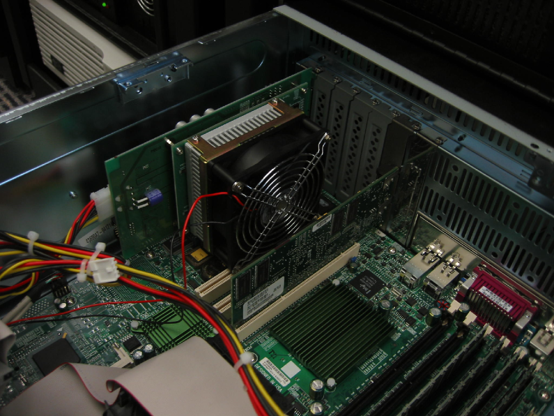
Figure 1: Interior of a node showing a GRAPE-6A card (note the large black fan) and an Infiniband card.

2.2 The GRAPE cluster

A computer cluster incorporating GRAPE-6A boards became fully operational at the Rochester Institute of Technology (RIT) in February 2005 (Fig. 2). This cluster, named “gravitySimulator,” consists of 32 compute nodes plus one head node each containing dual $3\,\mathrm{GHz}$-Xeon processors. In addition to a standard Gbit-ethernet, the nodes are connected via a low-latency Infiniband network with a transfer rate of $10\,\mathrm{Gbit}\,\mathrm{s}^{-1}$. The typical latency for an Infiniband network is of the order of $10^{-6}\,\mathrm{s}$, or a factor $\sim 100$ better then the Gbit-Ethernet (Liu et al. 2003). A total of 14 TByte of disk space is available on a level 5 RAID array. The disk space is equivalent to $2.5\times 10^{5}$ $N$-body data sets each with $10^{6}$ particles. The disks are accessed via a fast Ultra320 SCSI host adapter from the head node or via NFS from the compute nodes, which in addition are each fitted with a 80 Gbyte hard disk. Each compute node also contains a GRAPE-6A PCI card (Fig. 1). The total, theoretical peak performance is approximately $4\,\mathrm{TFlops}$ if the GRAPE boards are fully utilized. Total cost was roughly $0.45M, roughly 1/2 of which was used to purchase the GRAPE boards.

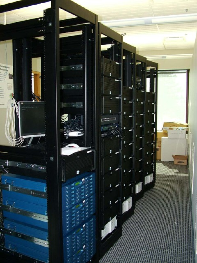
Figure 2: gravitySimulator, the GRAPE cluster at RIT. The head node and the 14 Tbyte raid array are visible on the first rack. The other four racks hold a total of 32 compute nodes, each equipped with a GRAPE-6A card.

Some special considerations were required in order to incorporate the GRAPE cards into the cluster. Since our GRAPE-6A’s use the relatively old PCI interface standard (32 bit/33 MHz), only one motherboard was found, the SuperMicro X5DPL-iGM, that could accept both the GRAPE-6A and the Infiniband card. (A newer version of the GRAPE-6A that uses the faster PCI-X technology is now available.) The PC case itself has to be tall enough (4U) to accept the GRAPE-6A card and must also allow good air flow for cooling since the GRAPE card is a substantial heat source. The cluster has a total power consumption of $17\,\mathrm{kW}$ when the GRAPEs are fully loaded. Cluster cooling was achieved at minimal cost by redirecting the air conditioning from a large room toward the air-intake side of the cluster. Temperatures measured in the PC case and at the two CPUs remain below 30 C and 50 C, respectively.

A similar cluster, called “GRACE” (GRAPE + MPRACE), was recently installed in the Astronomisches Rechen-institut (ARI) at the University of Heidelberg. There are two major differences between the RIT and ARI clusters. 1) Each node of the ARI cluster incorporates a reconfigurable FPGA card (called “MPRACE”) in addition to to the GRAPE board. MPRACE is optimized to compute neighbor forces and other, non-Newtonian forces between particles, in order to accelerate calculations of molecular dynamics, smoothed-particle hydrodynamics, etc. 2) The newer main board SuperMicro X6DAE-G2 was used, which supports Pentium Xeon chips with 64 bit technology (EM64T) and the PCIe (PCI express) bus. This made it possible to use dual-port Infiniband interconnects via the PCI express Infiniband x8 host interface card, used in the x16 Infiniband slot of the board (it has another x4 Infiniband slot which is reserved for the MPRACE-2 Infiniband card). As discussed below, the use of the PCIe bus substantially reduces communication overhead. Benchmark results presented below for the ARI cluster were obtained from algorithms that do not access the FPGA cards.

3 The parallel $N$-body code

We present here a new direct-summation code, called $\varphi$GRAPE, which was optimized for perfomance on GRAPE clusters. The algorithm employs a Hermite integration scheme (Makino and Aarseth 1992) with hierarchical, commensurate block time steps. Although comparable in complexity to – and inspired by – Aarseth’s serial NBODY1 code (Aarseth 1999), $\varphi$GRAPE was written “from scratch” for the RIT GRAPE cluster.

3.1 Integration scheme

In addition to position ${\bf x}_{i}$, velocity ${\bf v}_{i}$, acceleration ${\bf a}_{i}$, and time derivative of acceleration ${\bf\dot{a}}_{i}$, each particle $i$ has its own time $t_{i}$ and time step $\Delta t_{i}$.

Integration consists of the following steps:

1. The initial time steps are calculated from

   $$\Delta t_{i}=\eta_{s}\frac{|{\bf a}_{i}|}{|{\bf\dot{a}}_{i}|},$$ (1)

   where typically $\eta_{s}=0.01$ gives sufficient accuracy.

2. The system time $t$ is set to the minimum of all $t_{i}+\Delta t_{i}$ and all particles $i$ that have $t_{i}+\Delta t_{i}=t$ are selected as active particles. Note that “classical” $N$-body codes (Aarseth 1999, 2003) employ a sorted time-step list to select short time step particles efficiently. Such sorting is abandoned in favor of a search over all $N$ particles, which improves load balance in the parallel code due to the more random distribution of short and long step particles.

3. Positions and velocities at the new $t$ are predicted for all particles using

   $${\bf x}_{j,\mathrm{p}}={\bf x}_{j,0}+(t-t_{j}){\bf v}_{j,0}+\frac{(t-t_{j})^{2}}{2}{\bf a}_{j,0}+\frac{(t-t_{j})^{3}}{6}{\bf\dot{a}}_{j,0}$$ (2)

   and

   $${\bf v}_{j,\mathrm{p}}={\bf v}_{j,0}+(t-t_{j}){\bf a}_{j,0}+\frac{(t-t_{j})^{2}}{2}{\bf\dot{a}}_{j,0}.$$ (3)

   Here, the second subscript denotes a value given either at the beginning (0) or the end (1) of the current time step. All quantities used in the predictor can be calculated directly, i.e. no memory of a previous time step is required.

4. Acceleration and its time derivative are updated for active particles only according to

   $${\bf a}_{i,1}=\sum_{j\neq i}Gm_{j}\frac{{\bf r}_{ij}}{(r_{ij}^{2}+\epsilon^{2})^{(3/2)}}$$ (4)

   and

   $${\bf\dot{a}}_{i,1}=\sum_{j\neq i}Gm_{j}\left[\frac{{\bf v}_{ij}}{(r_{ij}^{2}+\epsilon^{2})^{(3/2)}}+\frac{3({\bf v}_{ij}\cdot{\bf r}_{ij}){\bf r}_{ij}}{(r_{ij}^{2}+\epsilon^{2})^{(5/2)}}\right],$$ (5)

   where

   $${\bf r}_{ij}={\bf x}_{j,p}-{\bf x}_{i,p},$$ (6)

   $${\bf v}_{ij}={\bf v}_{j,p}-{\bf v}_{i,p},$$ (7)

   and $\epsilon$ is the softening parameter.

5. Positions and velocities of active particles are corrected using

   $${\bf x}_{i,1}={\bf x}_{i,\mathrm{p}}+\frac{\Delta t_{i}^{4}}{24}\mathbf{a}^{(2)}_{i,0}+\frac{\Delta t_{i}^{5}}{120}\mathbf{a}^{(3)}_{i,0}$$ (8)

   and

   $${\bf v}_{i,1}={\bf v}_{i,\mathrm{p}}+\frac{\Delta t_{i}^{3}}{6}\mathbf{a}^{(2)}_{i,0}+\frac{\Delta t_{i}^{4}}{24}\mathbf{a}^{(3)}_{i,0},$$ (9)

   where the second and third time derivatives of ${\bf a}$ are given by

   $$\mathbf{a}^{(2)}_{i,0}=\frac{-6\left({\bf a}_{i,0}-{\bf a}_{i,1}\right)-\Delta t_{i}\left(4{\bf\dot{a}}_{i,0}+2{\bf\dot{a}}_{i,1}\right)}{\Delta t_{i}^{2}}$$ (10)

   $$\mathbf{a}^{(3)}_{i,0}=\frac{12\left({\bf a}_{i,0}-{\bf a}_{i,1}\right)+6\Delta t_{i}\left({\bf\dot{a}}_{i,0}+{\bf\dot{a}}_{i,1}\right)}{\Delta t_{i}^{3}}.$$ (11)

6. The times $t_{i}$ are updated and the new time steps $\Delta t_{i}$ are determined. Time steps are calculated using the standard formula (Aarseth 1985):

   $$\Delta t_{i,1}=\sqrt{\eta\displaystyle\frac{|{\bf a}_{i,1}||\mathbf{a}^{(2)}_{i,1}|+|{\bf\dot{a}}_{i,1}|^{2}}{|{\bf\dot{a}}_{i,1}||\mathbf{a}^{(3)}_{i,1}|+|\mathbf{a}^{(2)}_{i,1}|^{2}}}.$$ (12)

   The parameter $\eta$ controls the accuracy of the integration and is typically set to $0.02$. The value of $\mathbf{a}^{(2)}_{i,1}$ is calculated from

   $$\mathbf{a}^{(2)}_{i,1}=\mathbf{a}^{(2)}_{i,0}+\Delta t_{i,0}\mathbf{a}^{(3)}_{i,0}$$ (13)

   and $\mathbf{a}^{(3)}_{i,1}$ is set to $\mathbf{a}^{(3)}_{i,0}$.

7. Repeat from step (2).

A hierarchical commensurate block time step scheme is necessary when the Hermite integrator is used with the GRAPE (and is also efficient for parallelization and vectorization; see below and McMillan (1986)). Particles are grouped by replacing their time steps $\Delta t_{i}$ with a block time step $\Delta t_{i,\mathrm{b}}=(1/2)^{n}$, where $n$ is chosen according to

$$\left(\frac{1}{2}\right)^{n}\leq\Delta t_{i}<\left(\frac{1}{2}\right)^{n-1}.$$ (14)

The commensurability is enforced by requiring that $t/\Delta t_{i}$ be an integer. For numerical reason we also set a minimum time step $\Delta t_{\mathrm{min}}$, where typically

$$\Delta t_{\mathrm{min}}=2^{-23}.$$ (15)

The time steps of particles with $\Delta t_{i}<\Delta t_{\mathrm{min}}$ are set to this value. The minimum time step should be consistent with the maximum acceleration defined by the softening parameter; monitoring of the total energy can generally indicate whether this condition is being violated.

3.2 GRAPE implementation

The GRAPE-6 and GRAPE-6A hardware has been designed to work with a Hermite integration scheme and is therefore easily integrated into the algorithm described in the previous section (see Makino et al. 2003). In detail, integration of particle positions using the GRAPE-6A consists of the following steps:

1. Initialize the GRAPE and send particle data (positions, velocities, etc.) to GRAPE memory.
   

2. Compute the next system time $t$ and select active particles on the host (same as step 2 in previous section).
   

3. Predict postions and velocities of active particles only and send the predicted values together with the new system time $t$ to GRAPE’s force calculation pipeline.
   

4. Predict positions and velocities for all other particles on the GRAPE, and calculate forces and their time derivatives for active particles.
   

5. Retrieve forces and their time derivatives from the GRAPE and correct postions and velocities of active particles on the host.
   

6. Compute the new time steps and update the particle data on the host of all active particles in the GRAPE memeory.
   

7. Repeat from step (2).

3.3 Parallelization

Two basic schemes have been used to implement parallel force computations for $\mathcal{O}(N^{2})$ problems on general-purpose computers. The simplest case to consider is when all particles have the same fixed time step.

Replicated data algorithms (also called “copy” or “broadcast” algorithms). Each compute node has a copy of the whole system but is assigned a specific subset of $N/p$ particles, where $p$ is the number of processors. At every step, each node computes the forces exerted by all $N$ particles on its subset. These particles are then advanced and their updated positions and velocities are sent to the other processors.

Systolic algorithms (also called “ring” algorithms). At the start of the integration, each node is permanently assigned a subset of $N/p$ particles. At each step, these sub-arrays are shifted sequentially to the other nodes where the partial forces are computed and stored. After $p-1$ such shifts, all of the force pairs have been computed and the particles are returned to their original nodes where their trajectories can be advanced.

Both the replicated and systolic algorithms exhibit an $\mathcal{O}(N\log p)$ scaling in communication complexity and an $\mathcal{O}(N^{2})$ scaling in number of force computations. The systolic algorithm makes more efficient use of memory; however memory limitations are typically not restrictive for $N\mathrel{\mathchoice{\lower 3.6pt\vbox{\halign{$\mathsurround=0pt\displaystyle\hfil#\hfil$\cr<\crcr\sim\crcr}}}{\lower 3.6pt\vbox{\halign{$\mathsurround=0pt\textstyle\hfil#\hfil$\cr<\crcr\sim\crcr}}}{\lower 3.6pt\vbox{\halign{$\mathsurround=0pt\scriptstyle\hfil#\hfil$\cr<\crcr\sim\crcr}}}{\lower 3.6pt\vbox{\halign{$\mathsurround=0pt\scriptscriptstyle\hfil#\hfil$\cr<\crcr\sim\crcr}}}}10^{6}$ (Dorband et al. 2003; Gualandris et al. 2005).

The performance of parallel algorithms can be substantially degraded however if the $N$-body system has a “core-halo” structure, i.e. a dense central region surrounded by a low-density envelope. A galaxy containing a central black hole is an extreme example. Individual time steps (Equation 12) are mandated in this case, and the group size – the number of active particles due to be advanced at every time step – can be much smaller than $N$; indeed it can often be smaller than $p$. In the latter case, the systolic algorithm suffers since only a fraction of the nodes are active at a given time. Nonblocking communication is an effective way to deal with this problem since it allows communication to be put “in the background” so that computing nodes can send/receive data and calculate at the same time (Dorband et al. 2003).

Adding the GRAPE hardware imposes additional constraints. The GRAPE memory holds only $N_{G}\approx 10^{5}$ particles, hence the copy algorithm becomes inefficient for large $N$. The systolic algorithm is a natural alternative, allowing a total of $N_{G}\times p$ particles to be stored in the collective GRAPE memories. But a problem arises with the systolic algorithm if the number of active particles on any node is less than 48, since the time required by the GRAPE to compute forces on one particle is the same as the time to compute the forces on 48.

Our solution was to adopt a hybrid scheme. Nodes are initially assigned a subset of $N/p$ particles as in the systolic algorithm, where $N/p\leq N_{G}$, ensuring that all $N/p$ particles can be stored in the GRAPE memory. However, once the active particles on each node have been identified, they are broadcast to all the other nodes, thus minimizing the possibility that any one GRAPE will be required to compute forces on less than 48 particles.

In detail, our parallel algorithm works as follows:

1. Distribute the particle data to all nodes such that each node receives $N/p$ particles.
   

2. Initialize the GRAPE card on each node and send the local particle data to the GRAPE memories.
   

3. Compute the minimum time step on each node and use allreduce to find the global minimum.
   

4. Select the active particles on each node and predict their positions and velocities.
   

5. Collect the particle data (including the predicted values) of all active particles onto all nodes using allgather.
   

6. Compute the partial forces on each node for the global set of active particles using the GRAPE.
   

7. Retrieve the local partial forces, which are summed to get the total forces using allreduce.
   

8. Correct positions and velocities for the local active particles on each node and update the GRAPE memory.
   

9. Repeat from step (3).

4 Performance tests

We evaluated the performance of this algorithm on the two GRAPE clusters described above.

4.1 $N$-body models

Initial conditions for the performance tests were produced by generating Monte-Carlo positions and velocities from self-consistent models of stellar systems. Each of these models is spherical and is completely described by a steady-state phase-space distribution function $f(E)$ and its self-consistent potential $\Psi(r)$, where $E=v^{2}/2+\Psi$ is the particle energy and $r$ is the distance from the center. The models were: a Plummer (1911) sphere; two King (1966) models with different concentrations; and two Dehnen (1993) models with different central density slopes. The Plummer model has a low central concentration and a finite central density; it does not accurately represent any class of stellar system but is a common test case. King models are defined by a single dimensionless parameter $W_{0}$ describing the central concentration (e.g. ratio of central to mean density); we used $W_{0}=9$ and $W_{0}=12$ which are appropriate for globular star clusters (Spitzer 1987). Dehnen models have a divergent inner density profile, $\rho\propto r^{-\gamma}$. We took $\gamma=0.5$ and $\gamma=1.5$, which correspond approximately to the inner density profiles of bright and faint elliptical galaxies respectively (Gebhardt et al. 1996); in particular, the central bulge of the Milky Way galaxy has $\rho\sim r^{-1.5}$ (Genzel et al. 2003).

In what follows we adopt standard $N$-body units $G=M=-4E=1$, where $G$ is the gravitational constant, $M$ the total mass and $E$ the total energy of the system. In some of the models, the initial time step for some particles was smaller than the minimum time step $t_{\mathrm{min}}$ set in Eq. 15. These models were then rescaled to change the minimum time step to a large enough value. Since the rescaling does not influence the performance results we will present all results in the standard $N$-body units.

We realized each of the five models with 11 different particle numbers, $N=2^{k}$, $k=[10,11,...,20]$, i.e. $N=[1\,\mathrm{K},2\,\mathrm{K},...,1\,\mathrm{M}]$. We also tested Plummer models with $N=2\,\mathrm{M}$ and $N=4\,\mathrm{M}$; the latter value is the maximum $N$ value allowed by filling the memory of all 32 GRAPE cards. Thus, a total of 57 test models were used in the timing runs.

Figure 3: Energy conservation in each of the five test models, for four $N$-values. Relative errors have been shifted by multiples of $10^{-4}$ for each model. From top to bottom, each group of four lines represents Plummer models; Dehnen modes with $\gamma=0.5$ and $\gamma=1.5$; and King models with $W_{0}=9$ and $W_{0}=12$. The results for $N=4\,\mathrm{K}$ (full line), $64\,\mathrm{K}$ (dotted), $256\,\mathrm{K}$ (dashed) and $512\,\mathrm{K}$ (dash-dotted) are shown in each group.

Figure 4: Lagrange radii for Dehnen models ($\gamma=1.5$) with different $N$. The results for 4 096 (dotted), 131 072 (dashed) and 1 048 576 particles (full line) are shown. This is the densest (i.e. most centrally concentrated) of the test models are represents appoximately density profile of the Milky Way bulge. Lagrange radii of all other tested models were more stable.

Two-body relaxation, i.e. exchange of energy between particles due to gravitational scattering, induces a slow change in the characteristics of the models. In order to minimize the effects of these changes on the timing runs, we integrated the models for only one time unit. The softening $\epsilon$ was set to zero for the Plummer models and to $10^{-4}$ for the Dehnen and King models. The time step parameters were $\eta_{s}=0.01$ and $\eta=0.02$.

Figs. 3 and 4 show the dependence on time of the total energy, and the Lagrange radii, for the models. In all models, the maximum relative deviation in total energy is of the order of $10^{-5}$ or less. The Lagrange radii (shown only for Dehnen models with $\gamma=1.5$, the most centrally concentrated of the models which we considered) show that the mass profiles of all models remain practically unchanged. A noticable, but small, change in the innermost region can be seen only for the lowest particle numbers.

4.2 Performance results

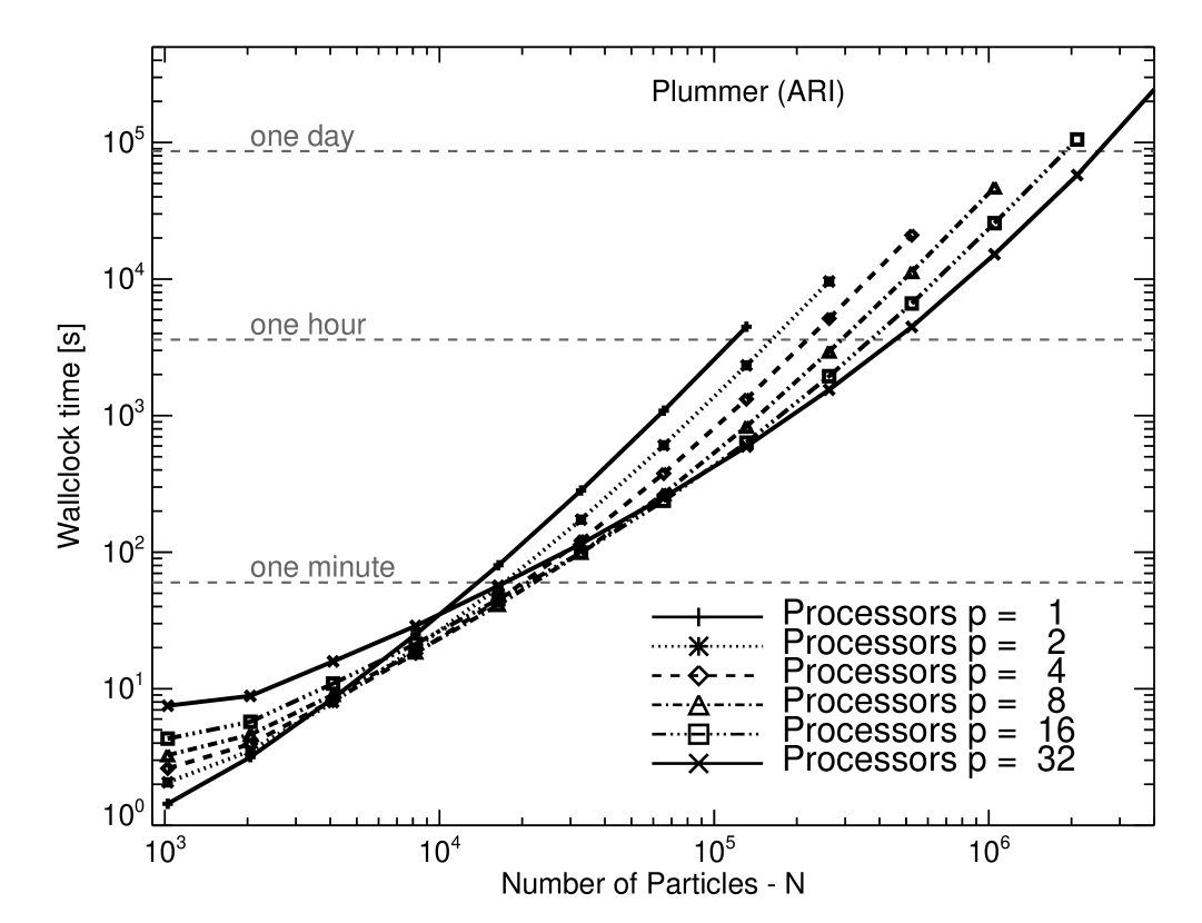
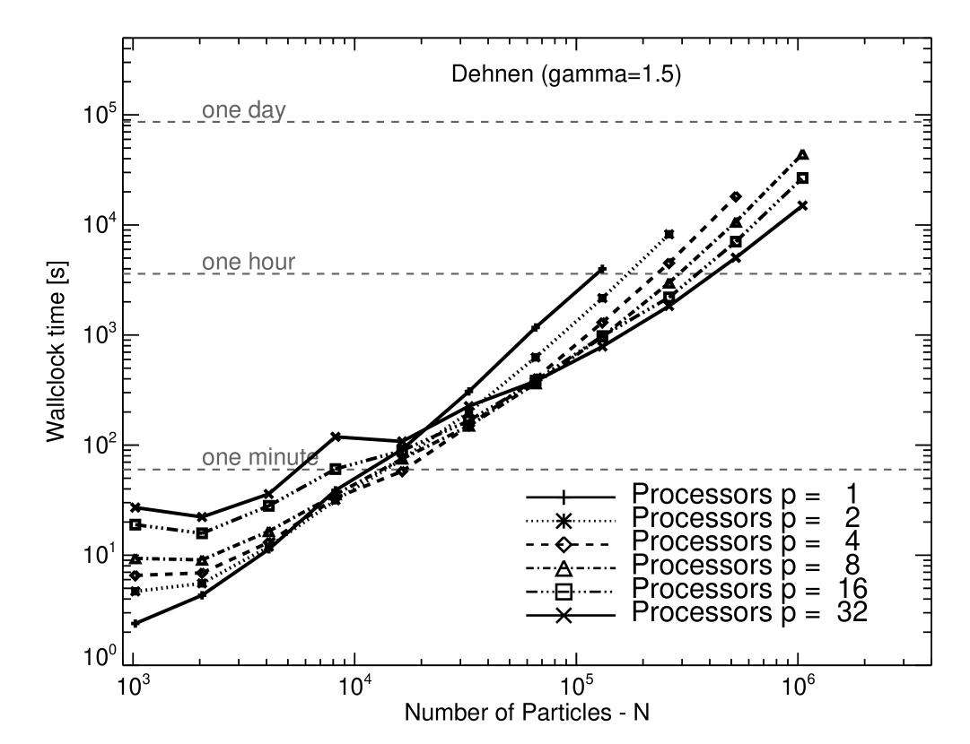
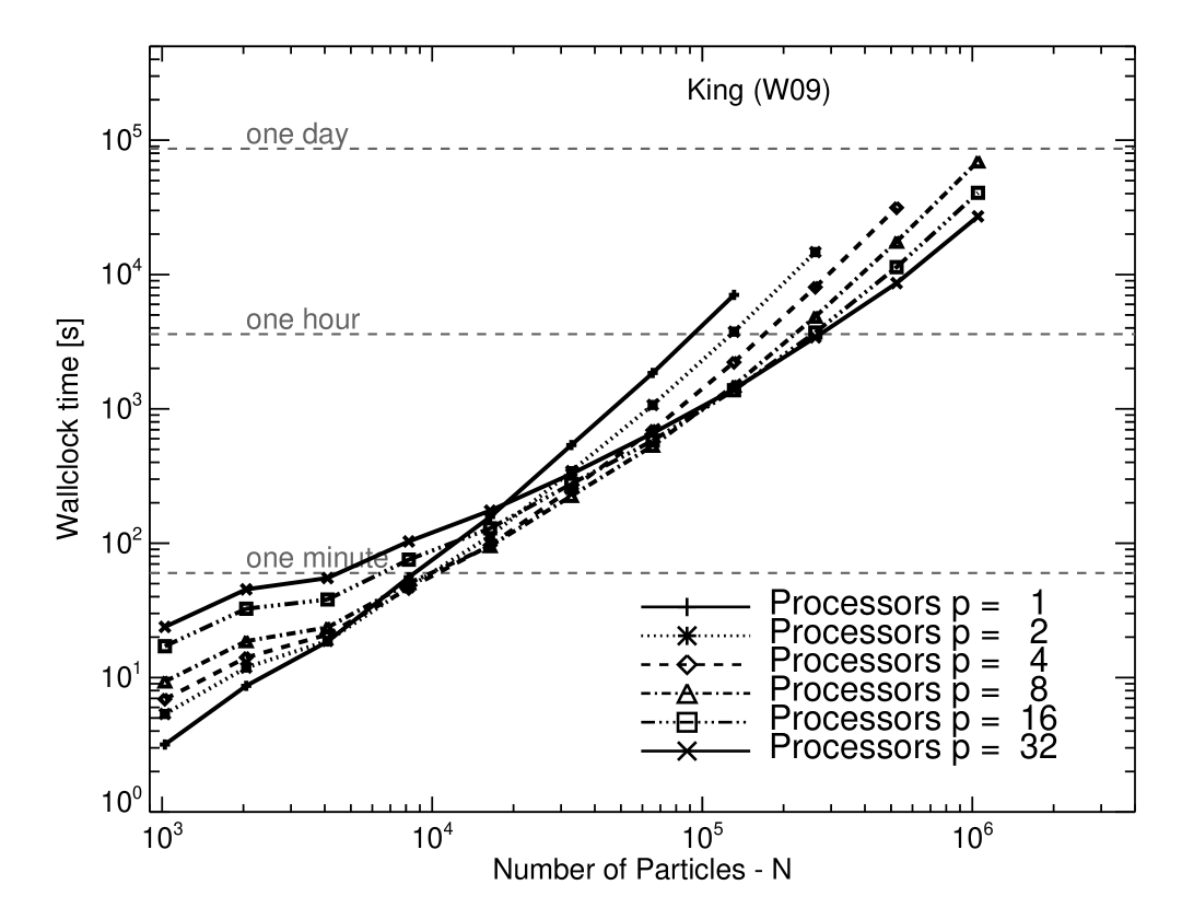
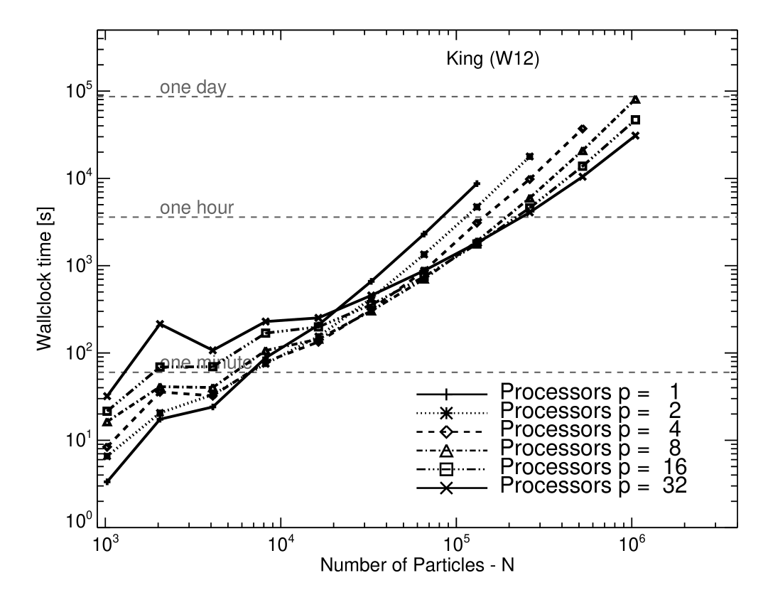
Figure 5: Wallclock time $w$ versus particle number $N$ for different numbers of processors $p$. The plots in the top row show the results for a Plummer model on the RIT (left) and ARI (right) clusters. The remaining plots show wallclock times of Dehnen models with $\gamma=0.5$ (middle left) and $\gamma=1.5$ (middle right) and of King models with $W_{0}=9$ (bottom left) and $W_{0}=12$ (bottom right).

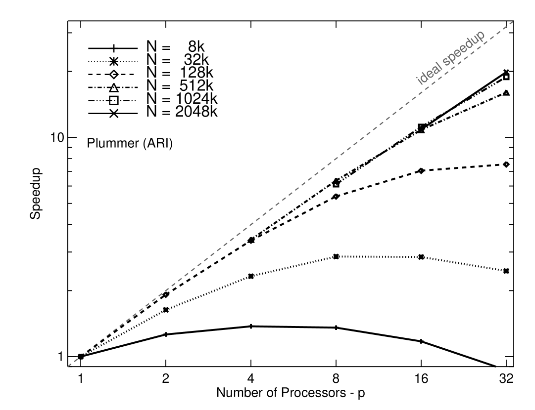
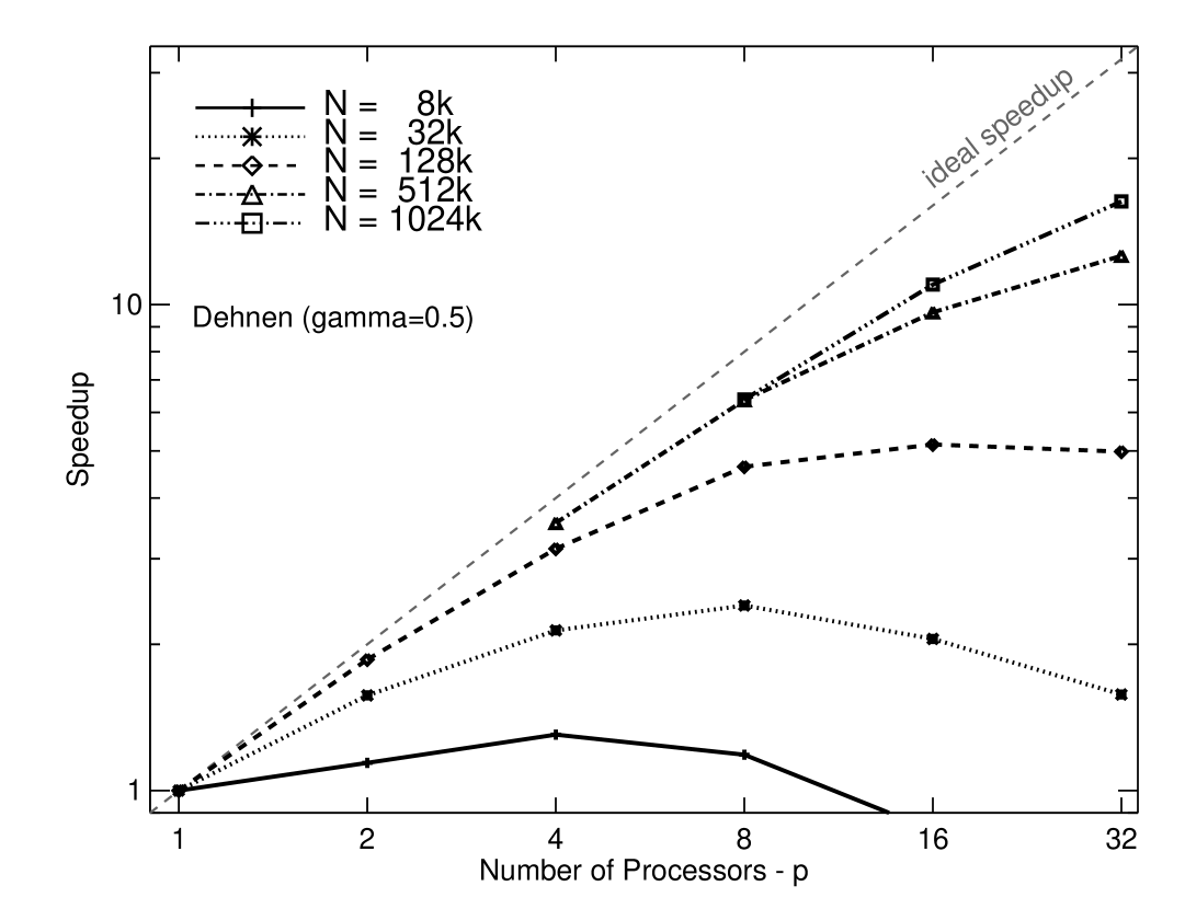
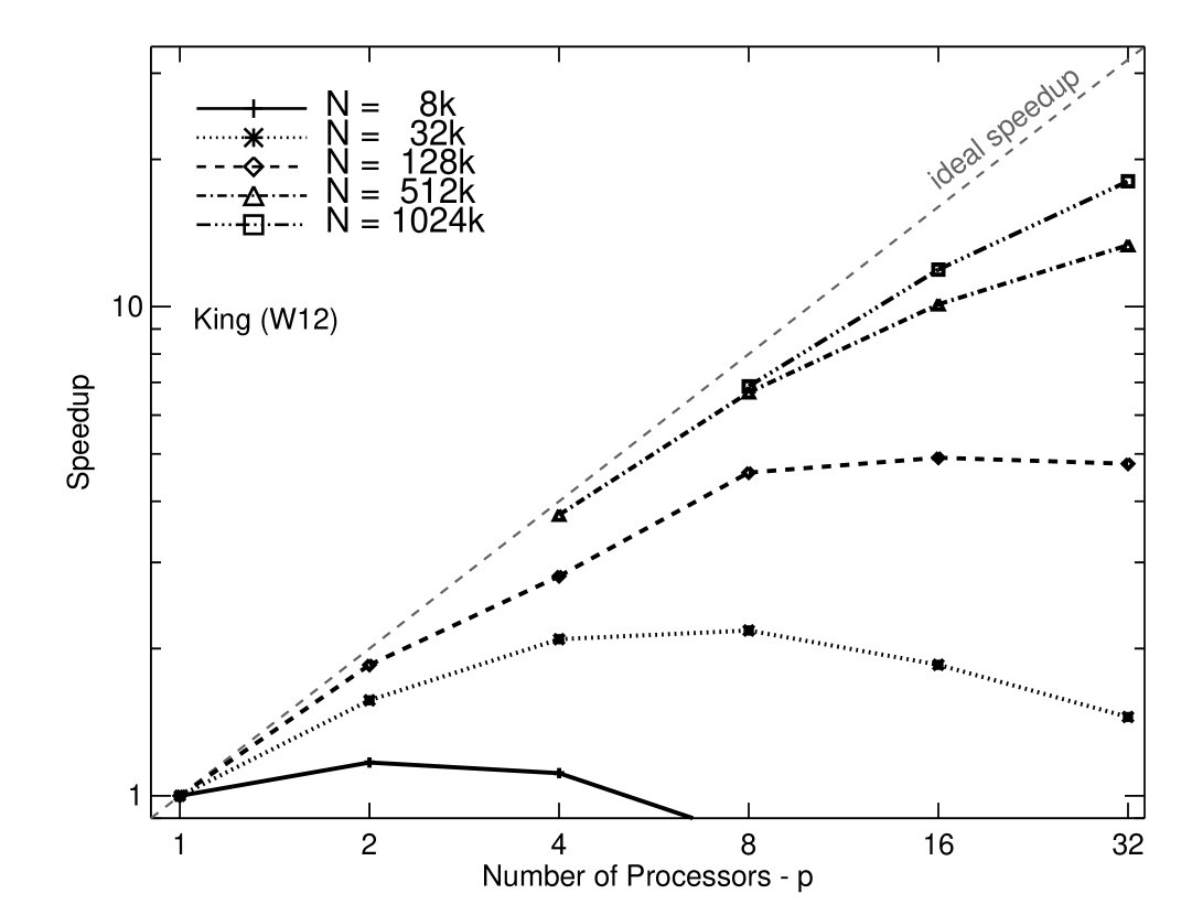
Figure 6: Speedup $s$ versus processor number $p$ for different particle numbers $N$. The plots in the top row show the results for a Plummer model on the RIT (left) and ARI (right) clusters. The remaining plots show the speedup for Dehnen models with $\gamma=0.5$ (middle left) and $\gamma=1.5$ (middle right) and for King models with $W_{0}=9$ (bottom left) and $W_{0}=12$ (bottom right).

Figure 7: Efficiency $e$ vs. number of processors $p$ for different particle numbers $N$. The plots in the top row show the results for a Plummer model on the RIT (left) and ARI (right) clusters. The remaining plots show efficiencies for Dehnen models with $\gamma=0.5$ (middle left) and $\gamma=1.5$ (middle right) and for King models with $W_{0}=9$ (bottom left) and $W_{0}=12$ (bottom right).

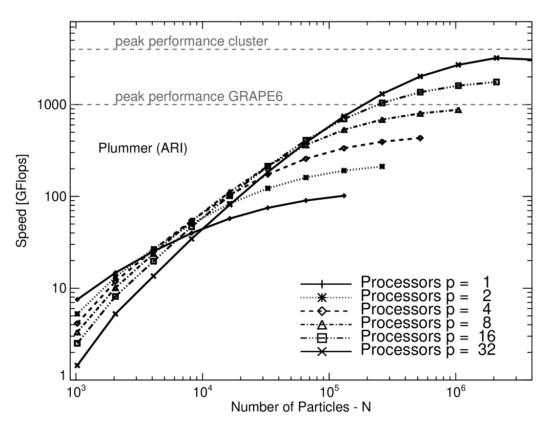
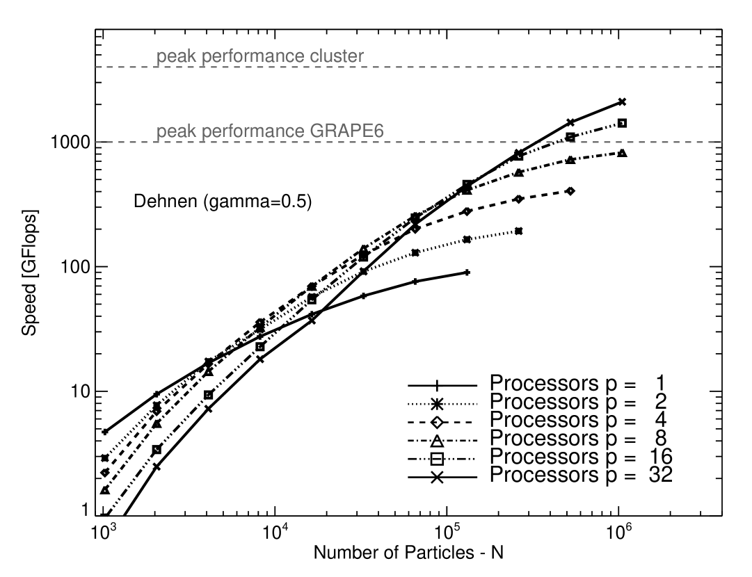
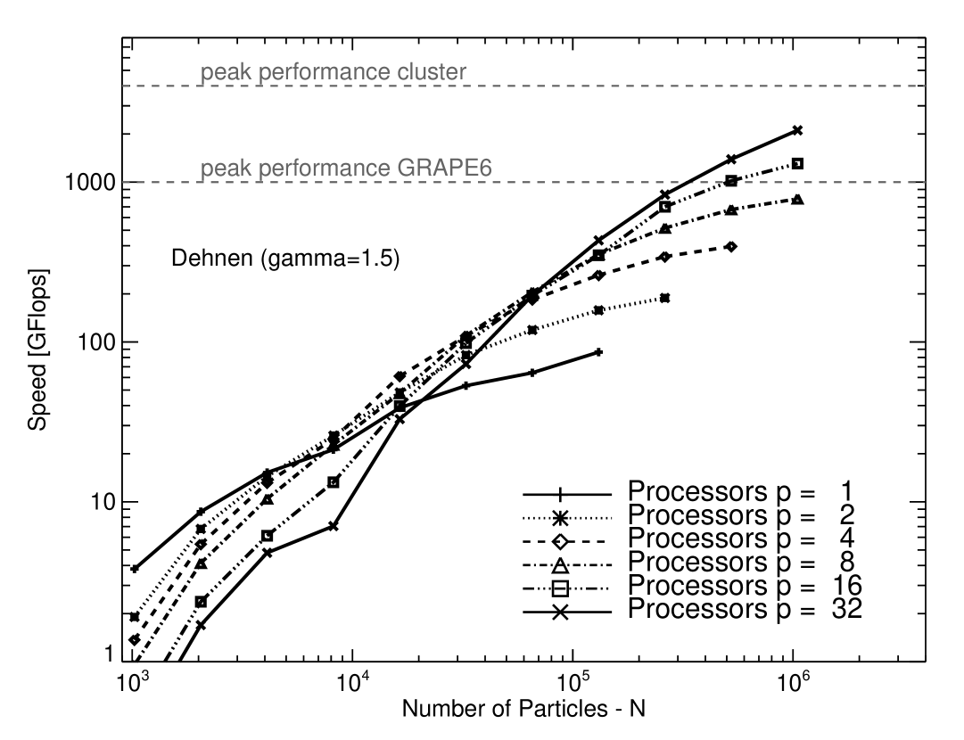
Figure 8: Speed $f$ vs. particle number $N$ for different numbers of processors $p$. The plots in the top row show the results for a Plummer model on the RIT (left) and ARI (right) clusters. The remaining plots show the speed for Dehnen models with $\gamma=0.5$ (middle left) and $\gamma=1.5$ (middle right) and for King models with $W_{0}=9$ (bottom left) and $W_{0}=12$ (bottom right).

Figure 9: Speed ratio $r$ vs. particle number $N$ for different numbers of processors $p$. The plots in the top row show the results for a Plummer model on the RIT (left) and ARI (right) clusters. The remaining plots show the speed ratio for Dehnen models with $\gamma=0.5$ (middle left) and $\gamma=1.5$ (middle right) and for King models with $W_{0}=9$ (bottom left) and $W_{0}=12$ (bottom right).

We analyzed the performance of the hybrid scheme as a function of particle number and also as a function of number of nodes; we used $p=1,2,4,8,16,$ and $32$ nodes. The compute time $w$ for a total of almost 350 test runs was measured using MPI_Wtime(). The timing was started after all particles had finished their initial time step and ended when the model had been evolved for one time unit. No data output was made during the timing interval.

Fig. 5 shows wallclock times $w_{N,p}$ from all integrations on the RIT cluster as a function of particle number $N$ and processor number $p$. We also show results from just the Plummer models on the ARI cluster. For any $p$, the clock time increases with $N$, roughly as $N^{2}$ for large $N$. However when $N$ is small, communication dominates the total clock time, and $w$ increases with increaing number of processors. This behavior changes as $N$ is increased; for $N\mathrel{\mathchoice{\lower 3.6pt\vbox{\halign{$\mathsurround=0pt\displaystyle\hfil#\hfil$\cr>\crcr\sim\crcr}}}{\lower 3.6pt\vbox{\halign{$\mathsurround=0pt\textstyle\hfil#\hfil$\cr>\crcr\sim\crcr}}}{\lower 3.6pt\vbox{\halign{$\mathsurround=0pt\scriptstyle\hfil#\hfil$\cr>\crcr\sim\crcr}}}{\lower 3.6pt\vbox{\halign{$\mathsurround=0pt\scriptscriptstyle\hfil#\hfil$\cr>\crcr\sim\crcr}}}}10\,\mathrm{K}$ (the precise value depends on the model), the clock time is found to be a decreasing function of $p$, indicating that the total time is dominated by force computations. The clock time is longer for the more centrally concentrated models since smaller time steps are required. As expected, the ARI cluster is faster than the RIT cluster by about 10% due to its newer hardware and better communication.

The centrally concentrated King and Dehnen models tend to have very small block sizes at small ($N\leq 10^{4}$) particle numbers. If such systems are integrated using the larger processor numbers, specific features related to the hardware and software implementation of communication (latencies) turn up, which are otherwise hidden by the dominating effect of large computation and communication, e.g. bandwidth and CPU speed. We will not discuss these effects in detail here although their influence can be discerned in the details of Figs. 5-9.

The speedup for selected test runs is shown in Fig. 6. Speedup $s$ is defined as

$$s_{N,p}=\frac{w_{N,1}}{w_{N,p}}.$$ (16)

The ideal speedup (optimal load distribution, zero communication and latency) is $s_{N,p}=p$. For particles numbers $N\mathrel{\mathchoice{\lower 3.6pt\vbox{\halign{$\mathsurround=0pt\displaystyle\hfil#\hfil$\cr>\crcr\sim\crcr}}}{\lower 3.6pt\vbox{\halign{$\mathsurround=0pt\textstyle\hfil#\hfil$\cr>\crcr\sim\crcr}}}{\lower 3.6pt\vbox{\halign{$\mathsurround=0pt\scriptstyle\hfil#\hfil$\cr>\crcr\sim\crcr}}}{\lower 3.6pt\vbox{\halign{$\mathsurround=0pt\scriptscriptstyle\hfil#\hfil$\cr>\crcr\sim\crcr}}}}128\,\mathrm{K}$ the wallclock time $w_{N,1}$ on one processor is undefined as $N$ exceeds the memory of the GRAPE card. In that case we used $w_{N,1}=w_{128\,\mathrm{K},1}\cdot(N/128\,\mathrm{K})^{2}$ assuming a simple $N^{2}$-scaling. In general, the speedup for any given particle number is roughly proportional to $p$ for small $p$, then reaches a maximum before dropping at large $p$. The number of processors at the the point of maximum speedup is “optimum” in the sense that it provides the fastest possible integration of the given problem. The optimum $p$ is roughly the value at which the sum of the communication and latency times equals the force computation time; in the zero-latency case, $p_{opt}\propto N$ (Dorband et al. 2003). Fig. 6 shows that for $N\mathrel{\mathchoice{\lower 3.6pt\vbox{\halign{$\mathsurround=0pt\displaystyle\hfil#\hfil$\cr>\crcr\sim\crcr}}}{\lower 3.6pt\vbox{\halign{$\mathsurround=0pt\textstyle\hfil#\hfil$\cr>\crcr\sim\crcr}}}{\lower 3.6pt\vbox{\halign{$\mathsurround=0pt\scriptstyle\hfil#\hfil$\cr>\crcr\sim\crcr}}}{\lower 3.6pt\vbox{\halign{$\mathsurround=0pt\scriptscriptstyle\hfil#\hfil$\cr>\crcr\sim\crcr}}}}128\,\mathrm{K}$, $p_{opt}\geq 32$ for all the tested models.

Efficiency (Fig. 7) $e$ is defined by

$$e_{N,p}=\frac{s_{N,p}}{p}.$$ (17)

Again, the comparison of the Plummer model on the clusters shows that the ARI cluster performs better. On 32 nodes the efficiency can be as high as $0.6$ for the highest $N$. Also, the efficiency does not vary much for models that have different central concentrations.

As mentioned before, the theoretical peak performance of a single GRAPE card (or node) is $f_{1,{\rm max}}\sim 131\,\mathrm{GFlops}$. We determined the compute speed $f$ from the measured total number of force updates $N_{f}$ in each run. For each force update $N$ forces are calculated, i.e. the compute speed is

$$f_{N,p}=57\cdot\frac{N\cdot N_{f}}{w_{N,p}},$$ (18)

which assumes $57$ floating point operations per force calculation. The measured compute speed is shown in Fig. 8. The maximum speeds reached are $2.2\,\mathrm{TFlops}$ on the RIT cluster and $3.2\,\mathrm{TFlops}$ on the ARI cluster.

The speed ratio $r$ is given by

$$r_{N,p}=\frac{f_{N,p}}{p\cdot f_{1,{\rm max}}}$$ (19)

and shown in Fig. 9. The speed ratio reached a maximum of $\sim 0.8$ and $\sim 0.9$ on the RIT and ARI clusters respectively. This shows again the benefits of the newer hardware in the ARI cluster. There are several reasons why the theoretical peak speed cannot be reached. Under a realistic time step distribution, it is impossible to keep the 48 pipelines on every GRAPE fully loaded. Evidence for this is seen in the lower speed ratios of the models with the more centrally-concentrated density distributions, like the Dehnen models, in which block sizes are typically small. In addition, the communication between the host and the GRAPE requires a non-negligible overhead of order of 10%. Communication also detracts from the performance; this can be seen in the slightly better performance of the ARI cluster, a result of its faster network.

5 Performance modeling

In this section we present a theoretical performance model for the execution time of a direct $N$-body code on a GRAPE cluster. We first consider the performance of a sequential code, which contains the essential elements of the performance of the GRAPE hardware, then consider the performance of the hybrid parallel scheme described in $\S\,$3.

5.1 Performance modeling of the sequential GRAPE code

If we consider a sequential block time-step code to be used in combination with GRAPE-6A, the time required to advance one active particle for one integration step can be written as

$$T\left(1\right)={T_{\rm host}}\left(1\right)+{T_{\rm grape}}\left(1\right)+{T_{\rm comm}}\left(1\right)$$ (20)

where ${T_{\rm host}}\left(1\right)={T_{\rm pred}}\left(1\right)+{T_{\rm corr}}\left(1\right)$ is the time spent on the host for the predictor and corrector operations, ${T_{\rm grape}}\left(1\right)=N\,{T_{\rm pipe}}$ is the time spent on the GRAPE for the force calculation and ${T_{\rm comm}}\left(1\right)$ is the time spent in communication between the host and the GRAPE. The communication time between GRAPE and host has three terms (Fukushige et al. 2005):

$${T_{\rm comm}}\left(1\right)=60\,t_{i}+56\,t_{f}+72\,t_{j}$$ (21)

where the first term represents the time to send the predicted positions and velocities to the GRAPE, the second term is the time to retrieve acceleration, jerk, and potential from the GRAPE, and the third term represents the time to send new data to the GRAPE memory for update. Table 1 reports the parameters measured on one GRAPE6-A of the RIT cluster.

The times ${T_{\rm pred}}$ for the predictor and ${T_{\rm corr}}$ for the corrector are measured on the host node. The parameter $t_{j}$ is derived by measuring the time $T_{\rm send}$ to send the data relative to one particle to the GRAPE memory: $t_{j}=T_{\rm send}/72$. We then assume $t_{i}=t_{f}=t_{j}$ as in Fukushige et al. (2005). The GRAPE parameter ${T_{\rm pipe}}$ is not measured directly but derived from the total time for the force calculation by subtracting the time for communication between the host and the GRAPE. This approach is necessary since the measured time $T_{\rm force}$ for the force calculation contains both the time for the force computation and the communication time between host and GRAPE. In this way ${T_{\rm pipe}}$ is given by ${T_{\rm pipe}}=\left(T_{\rm force}-\left(60\,t_{i}+56\,t_{f}\right)\right)/N$. The total wallclock time for one particle step is shown in Fig. 10 for different particle numbers, and compared with timing data on one GRAPE-6A. The agreement between the model and the data is very good for particle numbers larger than about 1K. For smaller $N$, there is a small deviation of the model from the data. The deviation is due to a slightly different value of ${T_{\rm pipe}}$ when the GRAPE memory holds a very small number of particles. Given the fact that we are not interested in such small particle numbers, we ignore this effect and consider a fixed ${T_{\rm pipe}}$ throughout our analysis.

Table 1: Performance parameters of one GRAPE-6A board

${T_{\rm pred}}\left(1\right)$	${T_{\rm corr}}\left(1\right)$	${T_{\rm pipe}}$	$t_{j}$
$(1.1\pm 0.2)\times 10^{-7}$	$(3.4\pm 0.3)\times 10^{-7}$	$(2.2\pm 0.5)\times 10^{-8}$	$(3.1\pm 0.5)\times 10^{-8}$

Figure 10: Time for one particle step as a function of the number of particles. The solid line indicates the theoretical prediction while the data points represent timing results on one GRAPE-6A.

The total time required to advance a block of active particles of size $s$ can then be written as

$$T\left(s\right)={T_{\rm host}}\left(s\right)+{T_{\rm grape}}\left(s\right)+{T_{\rm comm}}\left(s\right)$$ (22)

where

$${T_{\rm host}}\left(s\right) = {T_{\rm pred}}\left(s\right)+{T_{\rm corr}}\left(s\right)={T_{\rm host}}\left(1\right)\,s\,,$$

$${T_{\rm grape}}\left(s\right) = N\,{T_{\rm pipe}}\left[s/48\right]\,,$$

$${T_{\rm comm}}\left(s\right) = 60\,t_{i}s+56\,t_{f}s+72\,t_{j}s=188\,t_{j}s\,,$$ (23)

with $[x/y]=(\rm int)(x/y)+1$. Since the GRAPE pipeline accepts a maximum of 48 particles, ${T_{\rm grape}}$ is a step function with a step in correspondence of multiples of 48 in block size.

Fig. 11 shows a comparison between the predicted times (solid lines) for given block sizes $s$ and timing measurements (data points) conducted on the RIT cluster.

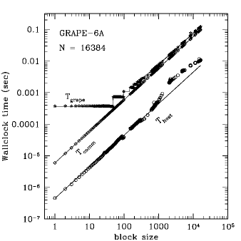
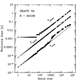
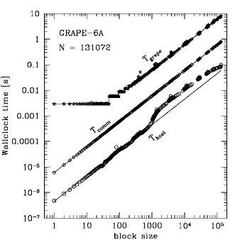
Figure 11: Times, predicted by the theoretical model, spent on the host, the GRAPE and in communication as a function of the block size for a sequential GRAPE code with block time steps. Data points are actual timing measurements on one GRAPE-6A of the RIT cluster.

The different plots refer to Plummer models with $N=8\,\mathrm{K},16\,\mathrm{K},64\,\mathrm{K},128\,\mathrm{K}$. Given the errors on the timing measurements and on the parameters reported in Table 1, there is good agreement between the data and the performance model. For the $N=8\,\mathrm{K}$ model, the time spent in communication between the host and the GRAPE is larger then the time spent on the GRAPE itself for the force calculation. For $N\gtrsim 16\,\mathrm{K}$, the time for the force calculation becomes larger then the communication time and for the $N=128\,\mathrm{K}$ system the total execution time is dominated by the force calculation on the GRAPE. This shows that the use of GRAPE hardware for $N$-body simulations is most efficient in the case of large systems, which are the most interesting from the scientific point of view. The non-linear increase in the host time for block sizes larger than about 1000 is likely due to cache misses.

The prediction and the measurements are independent of the chosen $N$-body model as long as the execution time is expressed as a function of the block size. In order to predict the execution time for the integration of a system over one $N$-body unit (or any other physical time), it is necessary to know the block size distribution for the model under consideration. In the case of a Plummer model with given $N$, the total execution time over one $N$-body time unit can be estimated by considering the average value of the block size $\langle s\rangle$ and the total number of integration steps $n_{\rm steps}$ in one $N$-body unit,

$$T_{N}=T_{N}(\langle s\rangle)\,n_{\rm steps}\,.$$ (24)

We have measured the average block size and the number of steps in one $N$-body unit for Plummer models of different $N$ and applied Eq. 24 to the prediction of the total execution times for the same models. Fig. 12 shows a comparison betweeen the predicted execution time for the integration of a Plummer model over one $N$-body unit and timing measurements on a single GRAPE-6A.

Figure 12: Comparison between the predictions by the theoretical model and the timing measurements for the integration of Plummer models over one $N$-body unit. The long-dashed line indicates the time spent on the GRAPE for the force calculation, the dotted line indicates the time spent in communication between the host and the GRAPE, the dashed line indicates the time spent on the host and the solid line represents the total execution time given by the sum of the three separate times. The data points indicate the results of the timing experiments conducted on a GRAPE-6A of the RIT cluster.

The model satisfactorily predicts the time spent on the host, on the GRAPE and in communication for particle numbers $N\gtrsim 2\,\mathrm{K}$. For smaller $N$, deviations from the prescription given by Eq. 24 are more likely to occur and to affect the modeling. In particular, the block size is generally small and the average is generally not a good representation of the global behavior of the system.

5.2 Performance modeling of the parallel GRAPE code

In the case of the hybrid scheme, the total execution time can be written as

$$T={T_{\rm host}}+{T_{\rm grape}}+{T_{\rm comm}}+{T_{\rm MPI}}$$ (25)

where ${T_{\rm MPI}}$ indicates the time spent in communication among the nodes. If $s$ is the block size at a specific step during the integration and $s_{\rm max}=\max_{i=1,\dots p}\left\{s_{i}\right\}$ is the maximum of the local blocks on the different nodes, the time spent on the host is given by

$${T_{\rm host}}={T_{\rm pred}}\left(s_{\rm max}\right)+{T_{\rm corr}}\left(s_{\rm max}\right)={T_{\rm pred}}\left(1\right)\,s_{\rm max}+{T_{\rm corr}}\left(1\right)\,s_{\rm max}\,,$$ (26)

the time spent on the GRAPE is given by

$${T_{\rm grape}}=\frac{N}{p}\,{T_{\rm pipe}}\left[s/48\right]\,,$$ (27)

the time spent in communication between the host and the GRAPE is

$${T_{\rm comm}}=60\,t_{i}s+56\,t_{f}s+72\,t_{j}\,s_{\rm max}\,,$$ (28)

and the time spent in communication among the nodes is given by the sum of the time spent in each MPI call. The time ${T_{\rm MPI}}$ is dominated by two calls to the function MPI_Allreduce and three calls to the function MPI_Allgatherv. We adopt the following models for the MPI functions:

$$T_{\tt MPI\_Allgatherv} = \left(\alpha+\beta\,x\right)log_{2}p,$$

$$T_{\tt MPI\_Allreduce} = \left(\delta+\gamma\,x\right)log_{2}p$$ (29)

where $x$ represents the size of transferred data measured in bytes and $\alpha$, $\beta$, $\delta$, $\gamma$ are parameters obtained by fitting timing measurements on the RIT cluster (see Table 2).

Table 2: Fit parameters for modeling of the MPI functions.

$\alpha$ [sec]	$\beta$ [sec]	$\delta$ [sec]	$\gamma$ [sec]
$1.2\times 10^{-5}$	$2.5\times 10^{-9}$	$1.0\times 10^{-5}$	$1.0\times 10^{-8}$

Fig. 13 reports the comparison between the prediction for the total execution time as a function of the block size at one specific step and the timing results on the RIT cluster. As in the case of the theoretical model, the times spent on the host, the GRAPE, in communication with the GRAPE and in communication among the nodes are measured separately and then added together.

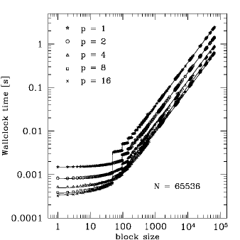
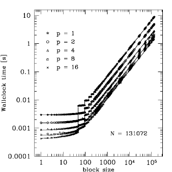
Figure 13: Comparison between the execution time predicted by the model for the integration of a Plummer model with $N$=65536 (left) and $N$ = 131072 (right) and timing experiments on the RIT cluster. The total execution time is plotted as a function of the block size.

In order to estimate the total execution time of the parallel scheme over one $N$-body unit, we consider the average value of the block size $\langle s\rangle$ and the total number of integration steps $n_{\rm steps}$ in one $N$-body unit for Plummer models with different particle numbers. Similarly to the case of the sequential code, we can approximate the total execution time for a particle number $N$ and processor number $p$ as

$$T_{N,p}=T_{N,p}(\langle s\rangle)~{}n_{\rm steps}\,.$$ (30)

Fig. 14 shows a comparison betweeen the predicted execution time for the integration of different Plummer models over one $N$-body unit and timing measurements.

Figure 14: Comparison between the predictions by the theoretical model (solid lines) and the timing measurements (data points) for the integration of Plummer models over one $N$-body unit. The different lines refer to different processor numbers.

For the theoretical prediction we have used Eq. 30 and measured values for the average block size and the number of steps in one $N$-body unit. The agreement between the model and the data is good for large particle numbers while deviations appear for small $N$.

6 Discussion

The performance of a direct-summation, parallel $N$-body code has been evaluated on two new computer clusters incorporating GRAPE special-purpose accelerator boards. Parallelization was carried out using a hybrid method incorporating aspects of both systolic (“ring”) and broadcast (“copy”) algorithms, in order to make the most efficient use of the GRAPE pipelines. The algorithm exhibits asymptotically an $\mathcal{O}(Np)$ scaling in communication complexity and an $\mathcal{O}(N^{2}/p)$ scaling in computation time. Benchmark simulations were carried out using a set of galaxy models having realistically high degrees of central concentration. Using one million particles and 32 nodes, the clusters achieved a sustained performance of 50% – 100% of the theoretical peak ($\sim 4\,\mathrm{TFlops}$). When run on general-purpose parallel computers, $N$-body codes like ours typically only achieve a few per cent of peak performance; hence, our special-purpose computer clusters are competitive with the fastest computers in the world when applied to the gravitational $N$-body problem.

We presented a simple model that predicts the performance of the $N$-body code as a function of processor number $p$, particle number $N$, and hardware constants. The model reproduces the observed performance very well, and can be used to predict the performance of the code on clusters with different hardware characteristics. The model supports our finding that the performance depends critically on having very fast and low-latency communication hardware.

It is convenient to discuss the performance of the parallel $N$-body code in terms of a working point $P$ defined by a pair of values $P=(p,N)$, where $P$ is given by the condition that the time required for communication and computation be approximately equal. When using all 32 of the processors on our clusters, this point is reached for $N\approx 10^{6}$. For larger $N$, the system operates at or near optimal speedup and efficiency (see Figs. 6 and 7). At a given $p$, the linear scaling of total computation time with $N$ at low $N$ (communication-dominated) changes to the asymptotic, $N^{2}$ scaling (computation dominated) roughly at $P$. Increasing $N$ beyond its value at $P$ would still achieve near-optimal speedups, but there would be room to increase $p$ without sacrificing efficiency (if more nodes were available). Increasing $p$ beyond $P$ at fixed $N$ is not useful because communication overhead will start to dominate, leaving the GRAPEs idle for part of the time. The design goal of our clusters was to simulate $\sim 10^{6}$ particles at high efficiencies, and we have shown by our performance tests that this goal has been achieved.

Figure 15: This figure demonstrates what particle numbers are needed to achieve the separation of time scales discussed in the text, when simulating nuclei containing a central sink, e.g. a single or binary BH. Vertical axis is the fraction of the flux into the “sink” originating from orbits that are in the empty-loss-cone regime; in real galaxies, this ratio is close to unity. Curves are labelled by $r_{LC}/r_{h}$, where $r_{LC}$ is the linear size of the central “sink” and $r_{h}$ is the BH influence radius. For a binary SBH, $0.1\leq r_{LC}/r_{h}\leq 10^{-3}$.

How large an $N$ is required to accurately represent the evolution of a dense stellar system like a galactic nucleus? A minimum condition is that $N$ be large enough to enforce a strict separation of time scales between the period $T_{orb}$ of an orbit and the relaxation time $T_{ref}$; the latter is the time for two-body gravitational scattering to randomize velocities (Spitzer 1987). In real galaxies, $T_{rel}\gg T_{orb}$, i.e. the integrity of stellar orbits is maintained for many orbital periods. In an $N$-body simulation, one has

$$T_{rel}\approx{0.1N\over\ln N}T_{orb}$$ (31)

(Aarseth 2003), and the separation of time scales can be achieved with modest particle numbers, $N\mathrel{\mathchoice{\lower 3.6pt\vbox{\halign{$\mathsurround=0pt\displaystyle\hfil#\hfil$\cr>\crcr\sim\crcr}}}{\lower 3.6pt\vbox{\halign{$\mathsurround=0pt\textstyle\hfil#\hfil$\cr>\crcr\sim\crcr}}}{\lower 3.6pt\vbox{\halign{$\mathsurround=0pt\scriptstyle\hfil#\hfil$\cr>\crcr\sim\crcr}}}{\lower 3.6pt\vbox{\halign{$\mathsurround=0pt\scriptscriptstyle\hfil#\hfil$\cr>\crcr\sim\crcr}}}}10^{3}$. Relaxation-driven processes like core collapse can be simulated using $N$-body codes and the numerical evolution rates scaled to those in real galaxies using an equation like (31) (Spurzem and Aarseth 1996; Szell et al. 2005).

In simulations of galactic nuclei, a much stronger separation of time scales must be achieved if the results are to be scaled to real systems, implying larger values of $N$. Galactic nuclei contain “sinks,” regions near the center where stars are lost or captured. For instance, the supermassive black hole (BH) at the center of the Milky Way galaxy disrupts stars that pass within a distance $r_{tidal}\approx 10^{-6}$ pc of it. Another example is a galaxy containing a binary supermassive BH: stars that pass within a distance $\sim a$ of either BH are ejected by the gravitational slingshot, where $10^{-3}\ {\rm pc}\mathrel{\mathchoice{\lower 3.6pt\vbox{\halign{$\mathsurround=0pt\displaystyle\hfil#\hfil$\cr<\crcr\sim\crcr}}}{\lower 3.6pt\vbox{\halign{$\mathsurround=0pt\textstyle\hfil#\hfil$\cr<\crcr\sim\crcr}}}{\lower 3.6pt\vbox{\halign{$\mathsurround=0pt\scriptstyle\hfil#\hfil$\cr<\crcr\sim\crcr}}}{\lower 3.6pt\vbox{\halign{$\mathsurround=0pt\scriptscriptstyle\hfil#\hfil$\cr<\crcr\sim\crcr}}}}a\mathrel{\mathchoice{\lower 3.6pt\vbox{\halign{$\mathsurround=0pt\displaystyle\hfil#\hfil$\cr<\crcr\sim\crcr}}}{\lower 3.6pt\vbox{\halign{$\mathsurround=0pt\textstyle\hfil#\hfil$\cr<\crcr\sim\crcr}}}{\lower 3.6pt\vbox{\halign{$\mathsurround=0pt\scriptstyle\hfil#\hfil$\cr<\crcr\sim\crcr}}}{\lower 3.6pt\vbox{\halign{$\mathsurround=0pt\scriptscriptstyle\hfil#\hfil$\cr<\crcr\sim\crcr}}}}10^{-1}$ pc is the semi-major axis of the binary. In this case, the radius of the “sink” is $\sim a\gg r_{tidal}$. Single or binary supermassive BHs are believed to be generic components of galaxies (Ferrarese and Ford 2005; Merritt and Milosavljević 2005), and the structure and evolution of nuclei may be shown to depend critically on the rate at which stars are lost to the central sink (Merritt 2006).

In real galaxies, relaxation times are long enough that most stars would diffuse gradually – i.e., over many orbital periods – onto so-called loss-cone orbits that intersect the capture sphere of radius $r_{tidal}$ or $a$. This means that the loss cone is essentially empty, since the removal time is much shorter than the diffusion time. In order to reproduce a diffusive loss-cone repopulation in an $N$-body simulation, the relaxation time must be large enough that

$$T_{rel}>\left({r\over r_{LC}}\right)T_{orb}\gg T_{orb}$$ (32)

(Lightman and Shapiro 1977). Here, $r_{LC}$ is the radius of the disruption ($\sim r_{tidal}$) or ejection ($\sim a$) sphere at the center of the galaxy, and $r$ is the typical size of a stellar orbit. Equation (32) reflects the fact that scattering into a loss-cone orbit occurs in much less than one relaxation time, hence maintaining an empty loss cone requires that relaxation times be much longer than orbital periods. This is a stricter condition than $T_{rel}\gg T_{orb}$ and implies a larger $N$.

Fig. 15 presents a more careful analysis along these lines. Shown there is the fraction of the flux into the central sink originating from orbits that are in the empty loss cone regime, as a function of $N$ and $r_{LC}$; the latter is expressed in units of $r_{h}$, the radius of gravitational influence of the central (single or binary) BH of mass $M_{\bullet}$. (The influence radius is the radius containing a mass in stars equal to twice $M_{\bullet}$.) In the case of a binary supermassive BH, $r_{LC}/r_{h}\approx a/r_{h}$ is roughly $10^{-1}$ at the time of binary formation, falling to $\sim 10^{-3}$ when the two BHs are close enough to coalesce. Fig. 15 suggests that particle numbers accessible to a single GRAPE-6 ($\sim 0.25$M) can only reproduce the empty loss cone regime characteristic of real galaxies during the early phases of binary evolution. The values of $N$ achievable on gravitySimulator ($\sim 4M$) allow the evolution of a binary to be followed to separations $\sim 1/10$ as small. These estimates are consistent with the results of recent simulations which reproduce diffusion-limited evolution of massive binaries with $N\approx 10^{6}$ (Makino and Funato 2004; Berczik et al. 2005). Simulating loss cone dynamics around the much smaller tidal disruption sphere of a single BH ($r_{LC}\approx 10^{-6}r_{h}$) would require considerably larger $N$, well beyond the capabilities of existing or planned computers. However the dynamics in this regime could be qualitatively reproduced by adjusting the size of the capture sphere in an $N$-body simulation such that the bulk of the stars scattered into the BH are on orbits respecting the correct ratio of $T_{rel}$ to $T_{orb}$.

The $T_{rel}\sim N$ scaling of Eq. (31) implies an effectively $\sim N^{3}$ scaling for calculations that extend over one relaxation time of the system. This scaling makes it very expensive to simulate the “collisional” evolution of stellar systems using the full, $4\times 10^{6}$ particle number allowed by the combined GRAPE memories on the RIT and ARI clusters. One way to accelerate the computations without significant loss of accuracy would be to use the Ahmad-Cohen (AC) neighbor scheme (Ahmad and Cohen 1973), as implemented in codes like NBODY5 or NBODY6 (Aarseth 1999). In the AC scheme, the full forces are computed only every tenth timestep or so; in the smaller intervals, the forces from nearby particles (the “irregular” force) are updated using a high order scheme, while those from the more distant ones (the “regular” force) are extrapolated using a second-degree polynomial. A parallel implementation of NBODY6, including the AC scheme, exists, but only for general-purpose parallel computers (Spurzem 1999; Khalisi et al. 2003); the algorithm has not yet been adapted to systems with GRAPE hardware.

Greater speedups could also be achieved by increasing the number $p$ of processors, but only if communication costs are held low. One way to do this is via a variant of the Lippert et al. (1998a, b) hyper-systolic (HS) algorithm. In its basic form, the HS algorithm reduces the number of data transfers by storing the shifted data on each node. The number of shifts, and hence the communication time, is reduced from $\mathcal{O}(p)$ to $\mathcal{O}(\sqrt{p})$ and the memory requirements are increased by a similar factor. The HS speedup is smaller when only a subset of the full $N$ particles are advanced at every time step however (Dorband et al. 2003). Makino (2002) has presented a direct $N$-body summation code optimized for a quadratic layout of processor ($p$ required to be a square number), which is in fact a simplified version of the hypersystolic algorithm proposed by Lippert et al. (1998b). In Makino’s case the asymptotic scaling of communication is $\mathcal{O}(N/\sqrt{p})$ (for calculation cost there is no difference to our code), which would allow to use much larger numbers of processors. However, performance tests of a HS $N$-body algorithm on actual hardware have apparently not been carried out.

Implementation of the AC and/or HS schemes should permit effective use of the RIT and ARI clusters with the full particle numbers permitted by the combined GRAPE memories. Still larger $N$ could be attained by implementing a hybrid scheme, e.g. coupling a direct-summation algorithm with a tree (McMillan and Aarseth 1993) or basis-function representation (Hemsendorf et al. 2002) for the distant particles, or a hierarchical generalization of the Ahmad-Cohen neighbor scheme.

References

- Aarseth (1985) Aarseth, S. J., 1985. Direct methods for N-body simulations. In: Brackbill, J. U., Cohen, B. I. (Eds.), Multiple Time Scales. p. 377.
- Aarseth (1999) Aarseth, S. J., Nov. 1999. From NBODY1 to NBODY6: The Growth of an Industry. PASP 111, 1333–1346.
- Aarseth (2003) Aarseth, S. J., 2003. Gravitational N-Body Simulations. ISBN 0521432723. Cambridge, UK: Cambridge University Press, November 2003.
- Ahmad and Cohen (1973) Ahmad, A., Cohen, L., Feb. 1973. Random Force in Gravitational Systems. ApJ 179, 885–896.
- Barnes and Hut (1986) Barnes, J., Hut, P., 1986. A Hierarchical O(NlogN) Force-Calculation Algorithm. Nature 324, 446–449.
- Berczik et al. (2005) Berczik, P., Merritt, D., Spurzem, R., Nov. 2005. Long-Term Evolution of Massive Black Hole Binaries. II. Binary Evolution in Low-Density Galaxies. ApJ 633, 680–687.
- Dehnen (1993) Dehnen, W., 1993. A Family of Potential-Density Pairs for Spherical Galaxies and Bulges. MNRAS 265, 250.
- Dorband et al. (2003) Dorband, E. N., Hemsendorf, M., Merritt, D., 2003. Systolic and hyper-systolic algorithms for the gravitational N-body problem, with an application to Brownian motion. Journal of Computational Physics 185, 484–511.
- Dubinski (1996) Dubinski, J., 1996. A parallel tree code. New Astronomy 1, 133–147.
- Efstathiou and Eastwood (1981) Efstathiou, G., Eastwood, J. W., 1981. On the clustering of particles in an expanding universe. MNRAS 194, 503–525.
- Ferrarese and Ford (2005) Ferrarese, L., Ford, H., 2005. Supermassive Black Holes in Galactic Nuclei: Past, Present and Future Research. Space Science Reviews 116, 523–624.
- Freitag and Benz (2001) Freitag, M., Benz, W., Aug. 2001. A new Monte Carlo code for star cluster simulations. I. Relaxation. A&A 375, 711–738.
- Fukushige et al. (2005) Fukushige, T., Makino, J., Kawai, A., 2005. GRAPE-6A: A Single-Card GRAPE-6 for Parallel PC-GRAPE Cluster Systems. PASJ 57, 1009–1021.
- Gebhardt et al. (1996) Gebhardt, K., Richstone, D., Ajhar, E. A., Lauer, T. R., Byun, Y.-I., Kormendy, J., Dressler, A., Faber, S. M., Grillmair, C., Tremaine, S., 1996. The Centers of Early-Type Galaxies With HST. III. Non-Parametric Recovery of Stellar Luminosity Distribution. AJ 112, 105.
- Genzel et al. (2003) Genzel, R., Schödel, R., Ott, T., Eisenhauer, F., Hofmann, R., Lehnert, M., Eckart, A., Alexander, T., Sternberg, A., Lenzen, R., Clénet, Y., Lacombe, F., Rouan, D., Renzini, A., Tacconi-Garman, L. E., 2003. The Stellar Cusp around the Supermassive Black Hole in the Galactic Center. ApJ 594, 812–832.
- Greengard and Rokhlin (1987) Greengard, L., Rokhlin, V., Dec. 1987. A fast algorithm for particle simulations. Journal of Computational Physics 73, 325–348.
- Gualandris et al. (2005) Gualandris, A., Portegies Zwart, S., Tirado-Ramos, A., 2005. Performance analysis of direct -body algorithsm on hghly distributed systems. In: IEEE 2004.
- Hemsendorf et al. (2002) Hemsendorf, M., Sigurdsson, S., Spurzem, R., Dec. 2002. Collisional Dynamics around Binary Black Holes in Galactic Centers. ApJ 581, 1256–1270.
- Khalisi et al. (2003) Khalisi, E., Omarov, C., Spurzem, R., Giersz, M., Lin, D., 2003. Collisional dynamics of black holes, star clusters and galactic nuclei. In: Krause, E., Jaeger, W., Resch, M. (Eds.), High Performance Computing in Science and Engineering ’03. Springer Verlag, pp. 71–87.
- King (1966) King, I. R., 1966. The structure of star clusters. IV. Photoelectric surface photometry in nine globular clusters. AJ 71, 276.