Determination of the atmospheric neutrino fluxes from experimental data

Abstract

The precise knowledge of the atmospheric neutrino fluxes is a key ingredient in the interpretation of the results from any atmospheric neutrino experiment. In the standard atmospheric neutrino data analysis, these fluxes are theoretical inputs obtained from sophisticated numerical calculations. In this work we present an alternative approach to the determination of the atmospheric neutrino fluxes based on the direct extraction from the experimental data on neutrino event rates.

1 Introduction

One of the most important breakthroughs in particle physics, and the only solid evidence for physics beyond the Standard Model, is the discovery – following a variety of independent experiments neutrev2 – that neutrinos are massive and consequently can oscillate among their different flavor eigenstates. The flavor oscillation hypothesis has been supported by an impressive wealth of experimental data, one of the most important pieces of evidence coming from atmospheric neutrinos.

Atmospheric neutrinos are originated by the collisions of cosmic rays with air nuclei in the Earth atmosphere. In the collision mostly pions (and some kaons) are produced and they subsequently decay into electron and muon neutrinos and anti-neutrinos. These neutrinos are observed in underground experiments using different techniques sk . In particular in the last ten years, high precision and large statistics data has been available from the SuperKamiokande experiment sk which has clearly established the existence of a deficit in the $\mu$-like atmospheric events with the expected distance and energy dependence from $\nu_{\mu}\rightarrow\nu_{\tau}$ oscillations with oscillation parameters $\Delta m^{2}\sim 2\times 10^{-3}$ eV² and $\tan^{2}\theta=1$. This evidence has also been confirmed by other atmospheric experiments such as MACRO and Soudan 2.

The expected number of atmospheric neutrino events depends on a variety of components: the atmospheric neutrino fluxes, the neutrino oscillation parameters and the neutrino-nucleus interaction cross section. Since the main focus of atmospheric neutrino data interpretation has been the determination of neutrino oscillation parameters, in the standard analysis the remaining components of the event rate computation are inputs taken from other sources. In particular, the fluxes of atmospheric neutrinos are taken from the results of numerical calculations, like those of Refs. honda ; bartol , which make use of a mixture of primary cosmic ray spectrum measurements, models for the hadronic interactions and simulation of particle propagation fluxrev .

The attainable accuracy in the independent determination of the relevant neutrino oscillation parameters from non-atmospheric neutrino experiments makes it possible to attempt an inversion of the strategy in the atmospheric neutrino analysis: to use the oscillation parameters as inputs in the data analysis in order to extract from data the atmospheric neutrino fluxes.

There are several motivations for such direct determination of the atmospheric neutrino flux from experimental data. First of all it would provide a cross-check of the standard flux calculations as well as of the size of the associated uncertainties (which being mostly theoretical are difficult to quantify). Second, a precise knowledge of atmospheric neutrino flux is of paramount importance for high energy neutrino telescopes icecubelect , both because they are the main background and they are used for detector calibration. Finally, such program will quantitatively expand the physics potential of future atmospheric neutrino experiments. Technically, however, this program is challenged by the absence of a generic parametrization of the energy and angular functional dependence of the fluxes which is valid in all the range of energies where there is available neutrino data.

In this contribution we present the first results on this alternative approach to the determination of the atmospheric neutrino fluxes: we will determine these fluxes from experimental data on atmospheric neutrino event rates, using all available information on neutrino oscillation parameters, cross-sections, as well as information from the different sources of experimental and theoretical uncertainty. The problem of the unknown functional form for the neutrino flux is bypassed by the use of neural networks as interpolants, since they allow us to parametrize the atmospheric neutrino flux without having to assume any functional behavior. Additional details on our approach can be found in paper .

Indeed the problem of the deconvolution of the atmospheric flux from experimental data on event rates is rather close in spirit to the determination of parton distribution functions in deep-inelastic scattering from experimentally measured structure functions qcdbook . For this reason, in this work we will apply for the determination of the atmospheric neutrino fluxes a general strategy originally designed to extract parton distributions in an unbiased way with faithful estimation of the uncertainties f2ns ; f2nnp ; pdf2 .

2 General strategy

The general strategy that will be used to determine the atmospheric neutrino fluxes was first presented in Ref. f2ns (see also nnthesis ). It involves two distinct stages in order to go from the data to the flux parametrization. In the first stage, a Monte Carlo sample of replicas of the experimental data on neutrino event rates (“artificial data”) is generated. These can be viewed as a sampling of the probability measure on the space of physical observables at the discrete points where data exist. In the second stage one uses neural networks to interpolate between points where data exist. In the present case, this second stage in turn consists of two sub-steps: the determination of the atmospheric event rates from the atmospheric flux in a fast and efficient way, and the comparison of the event rates thus computed to the data in order to tune the best-fit form of input neural flux distribution (“training of the neural network”). Combining these two steps, the space of physical observables is mapped onto the space of fluxes, so the experimental information on the former can be interpolated by neural networks in the latter.

In the present analysis we use the latest data on atmospheric neutrino event rates from the Super Kamiokande Collaboration sk . Higher energy data from neutrino telescopes like Amanda amandadata is not publicly available in a format which allows for its inclusion in the present analysis and its treatment is left for future work.

The latest Super Kamiokande atmospheric neutrino data sample is divided in 9 different types of events: contained events in three energy ranges, Sub-GeV, Mid-GeV and Multi-GeV electron- and muon-like, partially contained muon-like events and upgoing stopping and througoing muon events. Each of the above types of events is divided in 10 bins in the final state lepton zenith angle $\phi_{l}$. Therefore we have a total of $N_{\mathrm{dat}}=90$ experimental data points, which we label as

$$R_{i}^{(\exp)},\qquad i=1,\ldots,N_{\mathrm{dat}}\ .$$ (1)

Note that each type of atmospheric neutrino event rate is sensitive to a different region of the neutrino energy spectrum. In particular we note that for energies larger than $E_{\nu}\sim$ few TeV and smaller than $E_{\nu}\sim 0.1$ GeV there is essentially no information on the atmospheric flux from the available event rates.

The purpose of the artificial data generation is to produce a Monte Carlo set of ‘pseudo–data’, i.e. $N_{\mathrm{rep}}$ replicas of the original set of $N_{\mathrm{dat}}$ data points, $R^{(\mathrm{art})(k)}_{i}$ such that the $N_{\mathrm{rep}}$ sets of $N_{\mathrm{dat}}$ points are distributed according to an $N_{\mathrm{dat}}$–dimensional multi-gaussian distribution around the original points, with expectation values equal to the central experimental values, and error and covariance equal to the corresponding experimental quantities. This is achieved by defining

$$R_{i}^{(\mathrm{art})(k)}=R_{i}^{(\exp)}+r_{i}^{(k)}\sigma_{i}^{\mathrm{tot}}\ ,\quad k=1,N_{\mathrm{rep}}\ ,$$ (2)

where $N_{\mathrm{rep}}$ is the number of generated replicas of the experimental data, and where $r_{i}^{(k)}$ are univariate gaussian random numbers with the same correlation matrix as experimental data. We can then generate arbitrarily many sets of pseudo–data, and choose the number of sets $N_{\mathrm{rep}}$ in such a way that the properties of the Monte Carlo sample reproduce those of the original data set to arbitrary accuracy.

In our case each neural network parametrizes a neutrino flux. Since the precision of the available experimental data is not enough to allow for a separate determination of the energy, zenith angle and type dependence of the atmospheric flux, in this work we will assume the zenith and type dependence of the flux to be known with some precision and extract from the data only its energy dependence. That is, if $\mathrm{NN}\left(E_{\nu}\right)$ is the neural network output when the input is the neutrino energy $E_{\nu}$, then the neural flux parametrization will be

$$\Phi^{(\mathrm{net})}\left(E_{\nu},c_{\nu},t\right)=\mathrm{NN}\left(E_{\nu}\right)\Phi^{\mathrm{(ref)}}\left(E_{\nu},c_{\nu},t\right)\ .$$ (3)

$\Phi^{\mathrm{(ref)}}$ is a reference differential flux, which we take to be the most recent computations of either the Honda honda or the Bartol bartol collaborations, which have been extended to cover also the high-energy region by consistent matching with the Volkova fluxes.

Now let us describe a fast and efficient technique to evaluate the atmospheric neutrino event rates $R_{i}^{(\mathrm{net})}$ for an arbitrary input neural network atmospheric flux $\Phi^{(\mathrm{net})}\left(E_{\nu},c_{\nu},t\right)$. For example, for contained events any rate $R_{i}^{(\mathrm{net})}$ can be computed

$$R_{i}^{(\mathrm{net})}=n_{t}T\sum_{\alpha,\beta,\pm}\int_{0}^{\infty}dh\int_{-1}^{+1}dc_{\nu}\int_{E_{\mathrm{min}}}^{\infty}dE_{\nu}\int_{E_{\mathrm{min}}}^{E_{\nu}}dE_{l}$$

$$\int_{-1}^{+1}dc_{a}\int_{0}^{2\pi}d\varphi_{a}\frac{d^{3}\Phi_{\alpha}^{\pm(\mathrm{net})}}{dE_{\nu}\,dc_{\nu}\,dh}(E_{\nu},c_{\nu},h)$$

$$\,P_{\alpha\to\beta}^{\pm}(E_{\nu},c_{\nu},h\,|\,\vec{\eta})\,\frac{d^{2}\sigma_{\beta}^{\pm}}{dE_{l}\,dc_{a}}(E_{\nu},E_{l},c_{a})\,\varepsilon_{\beta}^{\text{bin}}(E_{l},c_{l})\,,$$ (4)

where $\Phi_{\alpha}^{+}$ ($\Phi_{\alpha}^{-}$) is the flux of atmospheric neutrinos (antineutrinos) of type $\alpha$, $\sigma_{\beta}^{+}$ ($\sigma_{\beta}^{-}$) is the charged-current neutrino- (antineutrino-) nucleon interaction cross section, and see statanal for a more detailed description of the above expression. The above expressions are very time-consuming to be evaluated, and this is specially a problem in our case since in the neural network approach one requires a very large number of evaluations.

However, the procedure can be speed up if one realizes that for a given flux, the expected event rates can always be written as

$$R_{i}=\sum_{t}\int_{-1}^{1}dc_{\nu}\int_{E_{\mathrm{min}}}^{\infty}dE_{\nu}\Phi\left(E_{\nu},c_{\nu},t\right)\widetilde{C}_{i}\left(E_{\nu},c_{\nu},t\right)\ ,$$ (5)

where $\widetilde{C}_{i}\left(E_{\nu},c_{\nu},t\right)$ contain all the $E_{\nu}$ and $c_{\nu}$ flux independent pieces in Eq.(4). Consequently if one discretizes the differential fluxes in $N_{e}$ energy intervals and $N_{z}$ zenith angle intervals

$$\Phi^{(\mathrm{net})}(E_{\nu},c_{\nu},t)=\sum_{e,z}\Psi_{ezt}^{(\mathrm{net})}\theta\left(E_{\nu}\in I_{e}\right)\theta\left(c_{\nu}\in I_{z}\right)\ ,$$ (6)

it is possible to write the theoretical predictions as a sum of the elements of a bin-integrated flux table $\Psi^{(\mathrm{net})}_{ezt}$,

$$R_{i}^{(\mathrm{net})}=\sum_{ezt}C^{i}_{ezt}\Psi^{(\mathrm{net})}_{ezt}\ ,$$ (7)

where the coefficients $C^{i}_{ezt}$, which are the most time-consuming ingredient, need only to be precomputed once before the training, since they do not depend on the parametrization of the atmospheric neutrino flux.

The determination of the parameters that define the neural network, its weights, is performed by maximum likelihood. This procedure, the so-called neural network training, proceeds by minimizing an error function, which coincides with the $\chi^{2}$ of the experimental points when compared to their theoretical determination obtained using the given set of fluxes:

$$E^{(k)}\left(\{\omega_{i}\}\right)=\mathrm{min}_{\vec{\xi}}\Bigg{[}\sum_{i,\mathrm{theo}}\xi^{2}_{i}+\sum_{i,\mathrm{sys}}\xi^{2}_{i}$$ (8)

$$\left(\sum_{n=1}^{N_{\mathrm{dat}}}\frac{R_{n}^{\mathrm{(\mathrm{net})(k)}}\left(\{\omega_{i}\}\right)\left[1+{\displaystyle\sum_{i}}\pi_{i}^{n}\xi_{i}\right]-R_{n}^{(\mathrm{art})(k)}}{\sigma_{n}^{\mathrm{stat}}}\right)^{2}\Bigg{]}\ .$$ (9)

The error function has to be minimized with respect to $\{\omega_{i}\}$, the parameters of the neural network. The minimization of Eq. (8) is performed with the use of genetic algorithms nnthesis . Because of the nonlinear dependence of the neural net on its parameters, and the nonlocal dependence of the measured quantities on the neural net (event rates are given by multi-dimensional convolutions of the initial flux distributions), a genetic algorithm turns out to be the most efficient minimization method.

Thus at the end of the procedure, we end up with $N_{\mathrm{rep}}$ fluxes, with each flux $\Phi^{(\mathrm{net})(k)}$ given by a neural net. The set of $N_{\mathrm{rep}}$ fluxes provide our best representation of the corresponding probability density in the space of atmospheric neutrino fluxes: for example, the mean value of the flux at a given value of $E_{\nu}$ is found by averaging over the replicas, and the uncertainty on this value is the variance of the values given by the replicas.

3 Results and discussion

Now we discuss the results of our determination of the atmosferic neutrino fluxes. Note that any functional of the neutrino flux (like for example event rates and its associated uncertainty) can be computed taking the appropriate moments over the constructed probability measure

$$\left\langle\mathcal{F}\left(\Phi\left(E_{\nu}\right)\right)\right\rangle_{\mathrm{rep}}=\frac{1}{N_{\mathrm{rep}}}\sum_{k=1}^{N_{\mathrm{rep}}}\mathcal{F}\left(\Phi^{(\mathrm{net})(k)}\left(E_{\nu}\right)\right)\ .$$ (10)

In Fig. 1 we show our results for the atmosferic neutrino flux as compared with the Honda and Bartol computations as well as with some direct measurements from Amanda amandadata . In Fig. 2 we show that the effects of the uncertainties in the neutrino oscillation parameters are rather small with respect the intrinsic flux uncertainties. Finally, we show in Fig. 3 how our neural network parametrization successfully reproduces the features of experimental data.

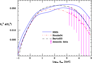
Figure 1: Comparison of the $1-\sigma$ uncertainty band of our parametrization of the atmospheric neutrino flux with recent computations and AMANDA data.

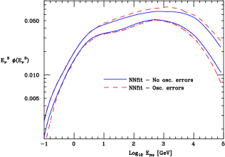
Figure 2: Results for fits varying the default neutrino oscillation parameters from their central values within their 1-$\sigma$ uncertainties globalfits .

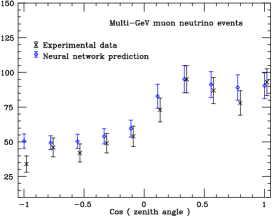
Figure 3: Comparison of the neural network results with experimental data for the Multi-GeV $\nu_{\mu}$ data sample.

The work presented in this contribution can be extended in several directions. First of all one could reduce the uncertainty in the large $E_{\nu}$ region by incorporating in the fit atmosferic neutrino measurements from neutrino detectors like Amanda amandadata . Second, we could use at even larger energies simple parametrizations of the flux to obtain a better estimation of backgrounds at neutrino telescopes. Finally, we could estimate the required statistics that would be required in forthcoming atmosferic neutrino experiments in order to determine from data also the zenith angle and flavor dependence of the neutrino flux.

References

- (1) Ashie, Y., et al.: A measurement of atmospheric neutrino oscillation parameters by super-kamiokande i. Phys. Rev. D71, 112,005 (2005)
- (2) Barr, G.D., Gaisser, T.K., Lipari, P., Robbins, S., Stanev, T.: A three-dimensional calculation of atmospheric neutrinos. Phys. Rev. D70, 023,006 (2004)
- (3) Del Debbio, L., Forte, S., Latorre, J.I., Piccione, A., Rojo, J.: Unbiased determination of the proton structure function f2(p) with faithful uncertainty estimation. JHEP 03, 080 (2005)
- (4) Del Debbio, L., Forte, S., Latorre, J.I., Piccione, A., Rojo, J.: The neural network approach to parton distribution functions: The nonsinglet case (In preparation)
- (5) Ellis, R.K., Stirling, W.J., Webber, B.R.: Qcd and collider physics. Camb. Monogr. Part. Phys. Nucl. Phys. Cosmol. 8, 1–435 (1996)
- (6) Forte, S., Garrido, L., Latorre, J.I., Piccione, A.: Neural network parametrization of deep-inelastic structure functions. JHEP 05, 062 (2002)
- (7) Gaisser, T.K., Honda, M.: Flux of atmospheric neutrinos. Ann. Rev. Nucl. Part. Sci. 52, 153–199 (2002)
- (8) Geenen, H.: Atmospheric neutrino and muon spectra measured with the amanda-ii detector (2003). Prepared for 28th International Cosmic Ray Conferences (ICRC 2003), Tsukuba, Japan, 31 Jul - 7 Aug 2003
- (9) Gonzalez-Garcia, C., Maltoni, M., Rojo, J.: Determination of atmospheric neutrino fluxes from atmospheric neutrino data. arxiv: hep-ph/0607324.
- (10) Gonzalez-Garcia, M.C., Maltoni, M.: Atmospheric neutrino oscillations and new physics. Phys. Rev. D70, 033,010 (2004)
- (11) Gonzalez-Garcia, M.C., Nir, Y.: Developments in neutrino physics. Rev. Mod. Phys. 75, 345–402 (2003)
- (12) Halzen, F.: Lectures on high-energy neutrino astronomy (2005)
- (13) Honda, M., Kajita, T., Kasahara, K., Midorikawa, S.: A new calculation of the atmospheric neutrino flux in a 3- dimensional scheme. Phys. Rev. D70, 043,008 (2004)
- (14) Maltoni, M., Schwetz, T., Tortola, M.A., Valle, J.W.F.: Status of global fits to neutrino oscillations. New J. Phys. 6, 122 (2004)
- (15) Rojo, J.: The neural network approach to parton distribution functions. Ph.D. thesis, Universitat de Barcelona (2006)
- (16) Rojo, J.: Neural network parametrization of the lepton energy spectrum in semileptonic b meson decays. JHEP 05, 040 (2006)
- (17) Rojo, J., Latorre, J.I.: Neural network parametrization of spectral functions from hadronic tau decays and determination of qcd vacuum condensates. JHEP 01, 055 (2004)