The intergalactic propagation of ultra-high energy cosmic ray nuclei

Abstract

We investigate the propagation of ultra-high energy cosmic ray nuclei ($A=1-56$) from cosmologically distant sources through the cosmic radiation backgrounds. Various models for the injected composition and spectrum and of the cosmic infrared background are studied using updated photodisintegration cross-sections. The observational data on the spectrum and the composition of ultra-high energy cosmic rays are jointly consistent with a model where all of the injected primary cosmic rays are iron nuclei (or a mixture of heavy and light nuclei).

I Introduction

The origin of the highest energy cosmic rays is among the most pressing questions in astroparticle physics Nagano:ve ; Anchordoqui:2002hs . The ultra-high energy cosmic ray (UHECR) spectrum has been measured, using both air shower and atmospheric fluorescence techniques, to energies beyond $10^{20}$ eV Lawrence:1991cc ; Bird:1994uy ; Takeda:1998ps ; Abu-Zayyad:2002sf . Protons of such high energies are not expected to be deflected significantly by galactic or extragalactic magnetic fields Dolag:2004kp , but should scatter inelastically on the cosmic microwave background (CMB) with an attenuation length of $\lesssim 30$ Mpc, i.e. about the size of the local supercluster of galaxies. The observed UHECRs do not point back to any plausible sources within this range and have an isotropic sky distribution, so their sources, if astrophysical, must be cosmologically distant. If so the spectrum should be suppressed at energies above $E_{\rm GZK}\sim 6\times 10^{19}$ eV (the “Greisen-Zatsepin-Kuzmin cutoff”), if the primaries are indeed protons Greisen:1966jv ; Zatsepin:1966jv . Presently, there are conflicting claims concerning the existence of this spectral feature. Data from AGASA (Akeno Giant Air Shower Array) show no indication of any suppression Takeda:1998ps , while data from the HiRes (High Resolution Fly’s Eye) air fluorescence detectors are consistent with the expected cutoff Abu-Zayyad:2002sf . The Pierre Auger Observatory, which employs both techniques, has accumulated an exposure comparable to AGASA and about half that of HiRes. Its results are presently consistent with either possibility Sommers:2005vs and forthcoming data should be able to settle the issue definitively. The AGASA observation that the spectrum continues smoothly beyond the GZK cutoff has motivated many suggestions for the origin of the trans-GZK events such as decaying superheavy dark matter particles in the Galactic halo Berezinsky:1997hy ; Birkel:1998nx and ultra-high energy neutrinos creating ‘Z-bursts’ in local interactions with the cosmic neutrino background Weiler:1997sh ; Fargion:1997ft . It has also been suggested that the primaries may be neutrinos with large interaction cross-sections at ultra-high energies Domokos:1998ry ; Jain:2000pu , or perhaps new stable strongly interacting particles heavier than the proton Albuquerque:1998va .

Rather less exotic ways of evading the GZK cutoff are also possible. In particular, if UHECRs are not protons but consist of heavy nuclei heavycase , then the spectrum will be altered from the usual expectation. Although evidence for the presence of heavy nuclei in UHECRs has been around for quite some time Bird:1993yi ; yakutsk ; earlyevidence , the information available on UHECR composition is still rather imprecise Watson:2004ew , the most reliable result being that the primaries are not mostly photons but hadrons Halzen:1994gy ; Shinozaki:2002ve ; Ave:2000nd ; Risse:2005hi . Despite the widespread impression to the contrary, however, there is little reason to believe that these particles are protons rather than heavier nuclei.

Determination of the mass composition of UHECRs has been attempted using a variety of variables such as the rate of change with primary energy of the depth of shower maximum $X_{\mathrm{max}}$, the degree of fluctuation in the depth of the shower maximum, the number of muons which reach the Earth’s surface, the lateral density profile with respect to the shower axis, the width of cosmic ray shower disks, etc. Such measurements must be compared to Monte Carlo simulations, typically conducted with programs such as QGSJET, SIBYLL and DPMJET Knapp:2002vs . The mass composition inferred is quite sensitive to the simulation program used. Furthermore, data from different experiments can yield rather different results regarding cosmic ray composition even when the same shower simulation is used. For example, at energies near $10^{18}$ eV, the mass composition determined from the lateral density profile of Volcano Ranch and Haverah Park data are in disagreement at $>2\sigma$ significance Dova:2004nq . The situation does not improve much at higher energies. Above $10^{19}$ eV, only the Fly’s Eye/HiRes and AGASA experiments have reported any information pertaining to mass composition, and these results extend to only about $2.5\times 10^{19}$ eV — in this energy range the data suggest a predominantly light composition although the uncertainties are large Abbasi:2004nz .

So far no individual sources of UHECRs have been identified. This can be understood if there are a very large number of faint sources or, alternatively, if there are large-scale magnetic fields which deflect UHECRs sufficiently so as to to conceal their origin. As mentioned above, protons at trans-GZK energies are not expected to be significantly deflected Dolag:2004kp (but see ref.Sigl:2003ay ). Heavy nuclei, by contrast, have greater electric charge and may thus have their arrival directions isotropised, even at such high energies.

There is also a theoretical prejudice to expect the UHECR spectrum to be dominated by heavy nuclei, since the maximum energy to which particles can be accelerated scales with the electric charge. Thus astrophysical candidates for UHECR accelerators such as active galactic nuclei and gamma-ray bursts, which barely meet the “Hillas criterion” hillas for containment and acceleration of $10^{20}$ eV protons, can in principle easily accelerate heavy nuclei to such energies.

Given these arguments, and the inconclusive nature of the experimental data regarding UHECR composition, it is rather surprising that most studies in this field have usually assumed that UHECRs are protons. By contrast, relatively little attention has been paid to the propagation of ultra-high energy nuclei Anchordoqui:1997rn ; Epele:1998ia ; Stecker:1998ib although there has been a resurgence of interest in recent years Bertone:2002ks ; Yamamoto:2003tn ; Khan:2004nd ; Armengaud:2004yt ; Allard:2005ha ; Sigl:2005md ; Allard:2005cx . We revisit this problem, using up-to-date nuclear physics data, and considering a wide range of nuclei as possible UHECR primaries. We also explore different models for the cosmic infrared background (CIB), as well as the effects of possible intergalactic magnetic fields. We pay particular attention to the relationship between the composition of UHECRs at Earth and that injected at source.

We begin by considering the intergalactic propagation of ultra-high energy (UHE) protons (Section II). In Sections III, IV and V, we study the photodisintegration of cosmic ray nuclei, including the effect of uncertainties in the cross-sections and the CIB model used. We then proceed to discuss the composition of UHECRs observed at Earth (Section VI), and the role of magnetic fields in the propagation of cosmic ray nuclei (Section VII). We propose some representative models of UHECR primary composition and discuss $X_{\mathrm{max}}$ measurements in Sections VIII and IX. Our conclusions are presented in Section X.

II Propagation of Ultra-High Energy Protons

Before discussing the propagation of intermediate mass and heavy nuclei, we first recapitulate the physics governing the propagation of UHE protons.

Over cosmological distances, the dominant processes effecting UHE proton propagation are interactions with the CMB producing pions or electron-positron pairs. Pair production ($p+\gamma_{\rm CMB}\rightarrow p+e^{+}+e^{-}$) occurs sufficiently frequently that it can be treated as a continuous energy loss process Blumenthal ; as shown in Figure 1 this effect dominates over the energy loss due to the Hubble expansion for proton energies $\sim 10^{18}-10^{21}$ eV and peaks at $\sim 3\times 10^{19}$ eV.

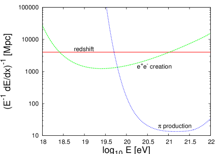
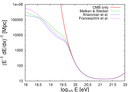
Figure 1: Energy loss lengths for UHE protons propagating through the universe. The left frame shows the results for the processes $p+\gamma_{\rm CMB}\rightarrow p+e^{+}+e^{-}$ (“$e^{+}e^{-}$ creation”), $p+\gamma_{\rm CMB}\rightarrow p+\pi^{0}$, $p+\gamma_{\rm CMB}\rightarrow n+\pi^{+}$ and multi-pion production (“$\pi$ production”), as well as due to the Hubble expansion (“redshift”). In the right frame, only pion production processes are considered and the effects of the cosmic infrared background (CIB) are shown in addition to the CMB (the three CIB models are discussed in Section IV).

Pion production is not as simple to implement. Individual occurrences of the processes $p+\gamma_{\rm CMB}\rightarrow p+\pi^{0}$ and $p+\gamma_{\rm CMB}\rightarrow n+\pi^{+}$ cause the primary proton to lose a considerable fraction of its energy. Therefore these cannot be treated as a continuous processes and it becomes necessary to use Monte Carlo techniques Mucke:1999yb . Furthermore, if enough energy is available, multi-pion production can be important; these non-perturbative processes take place through the near-resonance exchange of the 1.232 GeV $\Delta^{+}$-hadron pionsigma . The associated energy loss lengths are shown in Figure 1.

It is also possible for UHE protons to produce pions through interactions with the cosmic infrared background (CIB) as shown in the right frame of Figure 1. We show results for three models of the CIB which are discussed further in Section IV. Although the rates for these interactions are sub-dominant in comparison to energy losses from pair production, they can be important in determining the spectrum of “cosmogenic” neutrinos produced in UHE proton propagation Stanev:2004kz .

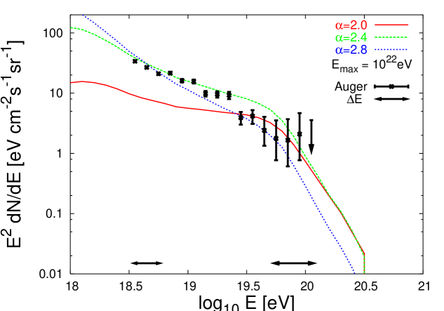
Figure 2: The UHECR spectrum at Earth for purely proton primaries injected by homogeneously distributed extragalactic sources with power law spectral indices of $\alpha=$ 2.0, 2.4 and 2.8 up to a maximum energy of $(E_{\rm max}/26)=(10^{22}$ eV/26) $\approx 10^{20.5}$ eV. The overall flux has in each case been normalized to the Auger data Sommers:2005vs (the $\chi^{2}$/d.o.f. for the fits are 9.97, 4.36, and 1.49 respectively). The effects of magnetic fields are not included.

For the injection spectrum, we follow previous work in adopting a simple power law with a cutoff:

$$\frac{dN_{p}}{dE_{p}}\propto E_{p}^{-\alpha},\qquad E_{p}<(E_{\rm max}/26).$$ (1)

Later in this paper, the quantity $E_{\mathrm{max}}$ will be used to describe the maximum energy to which iron nuclei can be accelerated by astrophysical sources. Since this maximum energy scales with the electric charge of the accelerated particle, protons have a cutoff energy 26 times smaller.

We also assume a constant comoving density of sources:

$$\frac{dN}{dV}\propto(1+z)^{3}.$$ (2)

The possible effects of source number evolution has also been considered, typically by adopting a distribution proportional to $(1+z)^{4}$. We find however that this has a negligible impact as UHECRs typically propagate over distances of only 10-100 Mpc (i.e. $z\ll 1$). In Figure 2, we show the UHECR spectrum expected at Earth for proton primaries — the “GZK cutoff” is clearly seen. It is also evident that none of these models fit the data well.

III photodisintegration of Ultra-High Energy Nuclei

The propagation of UHECRs is quite different in the case of heavy nuclei. These undergo photodisintegration in scattering off the CMB and/or CIB at a rate:

$$R_{A,Z,i_{p},i_{n}}=\frac{A^{2}m^{2}_{p}c^{2}}{2E^{2}}\int^{\infty}_{0}\frac{d\epsilon\,n(\epsilon)}{\epsilon^{2}}\int^{2E\epsilon/Am_{p}c}_{0}d\epsilon^{\prime}\epsilon^{\prime}\sigma_{A,Z,i_{p},i_{n}}(\epsilon^{\prime}),$$ (3)

where $A$ and $Z$ are the atomic number and charge of the nucleus, $i_{p}$ and $i_{n}$ are the numbers of protons and neutrons broken off from a nucleus in the interaction, $n(\epsilon)$ is the density of background photons of energy $\epsilon$, and $\sigma_{A,Z,i_{p},i_{n}}(\epsilon^{\prime})$ is the appropriate cross-section. (Note that $\epsilon$ is measured here in the laboratory rest frame, but in subsequent equations it refers to the energy measured in the rest frame of the nucleus.)

The cross-sections for photodisintegration have often been modelled using the parameterization of Stecker and collaborators Stecker:1969fw ; Puget:1976nz ; Stecker:1998ib :

$$\sigma_{A,i}(\epsilon)=\left\{\begin{array}[]{l@{\quad}l}\xi_{i}\Sigma_{\rm d}W_{i}^{-1}e^{-2(\epsilon-\epsilon_{p,i})^{2}/\Delta_{i}^{2}}\Theta_{+}(\epsilon_{\rm thr})\Theta_{-}(\epsilon_{1}),&\epsilon_{\rm thr}\leq\epsilon\leq\epsilon_{1},\quad i=1,2\\ \zeta\Sigma_{\rm d}\Theta_{+}(\epsilon_{\rm max})\Theta_{-}(\epsilon_{1})/(\epsilon_{\rm max}-\epsilon_{1}),&\epsilon_{1}<\epsilon\leq\epsilon_{\rm max}\\ 0,&\epsilon>\epsilon_{\rm max}\end{array}\right.$$ (4)

where $\xi_{i}$, $\zeta$, $\epsilon_{p,i}$ and $\Delta_{i}$ are parameters whose values are obtained by fitting to nuclear data. Here, $i$ is the total number of nucleons broken off from the nucleus in the interaction and the integrated cross-section is

$$\Sigma_{\rm d}\equiv\int_{0}^{\infty}\sigma(\epsilon)\,d\epsilon=\frac{2\pi^{2}e^{2}\hbar}{m_{p}c}\frac{(A-Z)Z}{A}=60\frac{(A-Z)Z}{A}\mbox{mb-MeV},$$ (5)

while the function $W_{i}$ is given by

$$W_{i}=\Delta_{i}\sqrt{\frac{\pi}{8}}\left[\mbox{erf}\left(\frac{\epsilon_{\rm max}-\epsilon_{p,i}}{\Delta_{i}/\sqrt{2}}\right)+\mbox{erf}\left(\frac{\epsilon_{p,i}-\epsilon_{1}}{\Delta_{i}/\sqrt{2}}\right)\right].$$ (6)

Here $\Theta_{+}(x)$ and $\Theta_{-}(x)$ are the Heaviside step functions, $\epsilon_{1}$ = 30 MeV, $\epsilon_{\rm max}$ = 150 MeV, and the threshold energy for a given process is in most cases $\epsilon_{\rm thr}\approx i\times 10$ MeV (values are tabulated in Ref. Stecker:1998ib ). These cross-sections are dominated by the giant dipole resonance which peaks in the energy range $\sim 10-30$ MeV; at higher energies, quasi-deuteron emission is the main process.

This model incorporates two major approximations. First, a simple Gaussian form is assumed for the photodisintegration cross-section, cut off abruptly below the theoretical reaction threshold. Second, a fixed choice of $Z$ is made for each given atomic number,$A$, thus neglecting the many possible isotopes which may be generated in such interactions.

Although this parametrization does a fairly good job of reproducing the measured cross-sections, possible improvements have been proposed. In particular, a generalized Lorentzian model, which can be fitted to the available nuclear data, has been used to parametrize a wide range of photodisintegration cross-sections Khan:2004nd :

$$\sigma_{A,Z,i_{p},i_{n}}(\epsilon_{\gamma})=\frac{\Gamma_{A,Z,i_{p},i_{n}}(\epsilon_{\gamma})\,\epsilon_{\gamma}^{4}}{(\epsilon_{\gamma}^{2}-E_{A,Z,i_{p},i_{n}}^{2})^{2}+\Gamma_{A,Z,i_{p},i_{n}}^{2}(\epsilon_{\gamma})\,\epsilon_{\gamma}^{2}}.$$ (7)

Here $E_{A,Z,i_{p},i_{n}}$ is the position of the giant dipole resonance and $\Gamma_{A,Z,i_{p},i_{n}}$ is the width of that resonance, given by

$$\Gamma_{A,Z,i_{p},i_{n}}(\epsilon_{\gamma})=\Gamma_{A,Z,i_{p},i_{n}}(E_{A,Z,i_{p},i_{n}})\,\frac{\epsilon_{\gamma}^{2}}{E_{A,Z,i_{p},i_{n}}^{2}}.$$ (8)

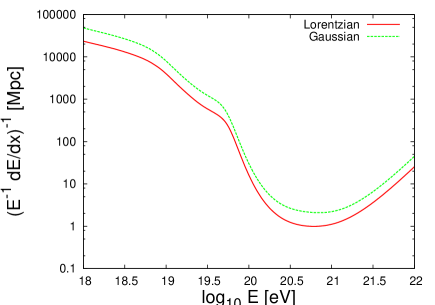
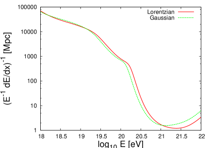
Figure 3: Energy loss lengths for photodisintegration of oxygen (left) and iron (right) nuclei on the CMB and CIB for both Gaussian and Lorentzian parameterizations of the cross-section. The CIB has been modelled according to Malkan & Stecker Malkan:2000gu (see Section IV).

In some cases, the Lorentzian form can be quite different from the Gaussian parameterization. In particular, the latter often overestimates the width of the giant dipole resonance. Despite these differences we find, as shown in Figure 3, that the energy loss rates due to photodisintegration change little whether we use the Gaussian model Stecker:1998ib or the Lorentzian model Khan:2004nd for nuclei between $A=11$ and 56 — henceforth we adopt the Lorentzian model. (Below this mass range, we use the Gaussian parameterization.)

IV The Cosmic Infrared Background

Since photodisintegration processes occur most efficiently when the Lorentz-boosted target photon can excite the giant dipole resonance at $\sim 10$ MeV, an UHE nucleus with an energy of $10^{19}$ eV (i.e. a Lorentz factor of $\sim 10^{8}-10^{9}$) needs to collide with a $\sim 0.01-0.1$ eV background photon in order to most efficiently undergo photodisintegration. Photons of this energy, corresponding to wavelengths of $\lambda\sim 10-100\,\mu$m, are present in the CIB rather than in the CMB.

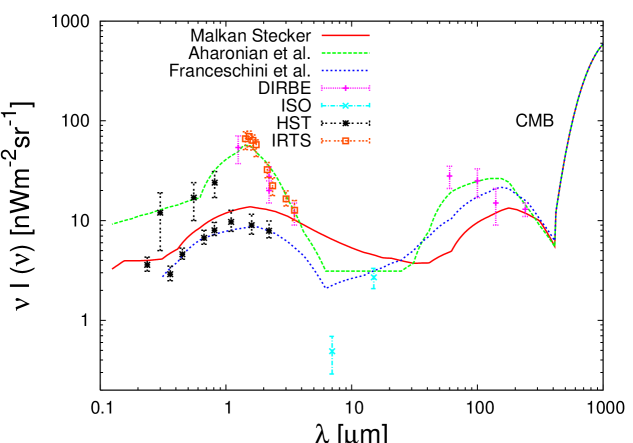
Figure 4: Representative models of the CIB spectrum from Malkan & Stecker Malkan:2000gu , Aharonian et al. Aharonian:2003wu and Franceschini et al. Franceschini:2001yg . Data shown are from DIRBE Hauser:2001xs , ISO Metcalfe:2003zi , HST Madau:1999yh ; Bernstein:2001rz ; Gard and IRTS irts .

The CIB is an expected relic of the cosmological structure formation processes Hauser:2001xs . The assembly of baryonic matter into stars and galaxies and the subsequent evolution of such systems is accompanied by the release of radiant energy; cosmic expansion and the absorption of short wavelength radiation by dust and re-emission at longer wavelengths shifts a significant part of this radiant energy into the infrared: $\lambda\sim$ 1-1000 $\mu$m. Thus the CIB spectrum depends on the luminosity and evolution of the sources and distribution of dust from which it is scattered.

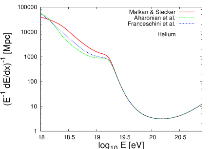
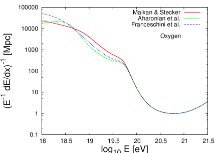
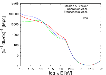
Figure 5: Energy loss lengths due to photodisintegration for helium, oxygen and iron nuclei for three models of the CIB spectrum. The Lorentzian model Khan:2004nd for photodisintegration cross-sections, been used.

Direct measurement of the CIB has been performed by several satellites, in particular the COsmic Background Explorer (COBE) and the InfraRed Telescope inSpace (IRTS). DIRBE, an instrument aboard the COBE satellite Hauser:1998ri , has provided measurements in the wavelength range 1.25–240 $\mu$m. FIRAS, another instrument aboard COBE, covered the range 25 $\mu$m – 1 mm. The ISO satellite carried two instruments which were employed in the indirect measurement of the CIB: ISOCAM at 7 and 15 $\mu$m and ISOPHOT at 170 $\mu$m Metcalfe:2003zi .

In addition to these measurements, telescopes such as the Hubble Space Telescope’s (HST) wide field planetary camera, combined with spectrophotometry from the duPont telescope and the HST Faint Object Spectrograph, were used to measure the CIB at 0.3, 0.55 and 0.8 $\mu$m. Galaxy counts made using the HST Northern and Southern Deep Fields, between 0.36 and 2.2 $\mu$m, supplemented with shallower ground based observations, have also been used to set lower limits on the CIB Madau:1999yh ; Bernstein:2001rz ; Gard .

We have considered three forms for the CIB spectrum which bracket the range of possibilities, The first is based on a compilation of the direct observations by Aharonian et al Aharonian:2003wu which is the uppermost curve at 1 $\mu$m in Figure 4. The second, from Franceschini et al. Franceschini:2001yg , corresponds roughly to the lower limit set by galaxy counts. The third is the empirical model by Malkan & Stecker Malkan:2000gu which lies between the other two curves (although at 100 $\mu$m it goes below the Franceschini et al. model). The observational data are also shown for comparison.

In Figure 5, we show the effect of our choice of the CIB spectrum on the energy loss rates of cosmic ray nuclei through photodisintegration. It is clear that the choice makes a substantial difference only for particularly heavy nuclei. Henceforth, unless otherwise stated, we will adopt the Malkan & Stecker model Malkan:2000gu for the CIB spectrum. We note that this spectrum is consistent with recent observations by HESS of TeV $\gamma$-rays from distant blazars which imply restrictive upper bounds on the CIB and suggest that the direct observations in the $\sim 1-10~{}\mu$m range may well have been contaminated by zodiacal light Aharonian:2006fe .

V Propagation of Ultra-High Energy Nuclei

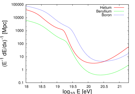
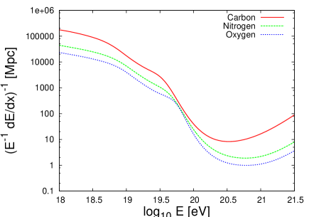
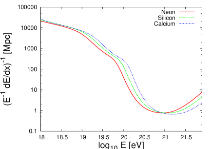
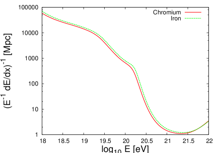
Figure 6: Energy loss lengths due to photodisintegration for a range of intermediate mass and heavy nuclei. The Malkan & Stecker CIB model Malkan:2000gu and the Lorentzian model Khan:2004nd for photodisintegration cross-sections have been used.

Now we can study the intergalactic propagation of UHE nuclei and determine the UHECR spectrum at Earth for various types of nuclei injected at source. In Figure 6 we plot the energy loss length due to photodisintegration for several nuclei species. It is seen that there are significant variations, for example, carbon nuclei are relatively robust to photodisintegration with an energy loss length of $\sim 50$ Mpc at $10^{20}$ eV and several thousand Mpc at $3\times 10^{19}$ eV, while beryllium nuclei are highly fragile, with an energy loss length smaller by a factor of $\sim 10-100$. Very heavy nuclei are generally quite stable up to energies $\sim 10^{20}$ eV.

In practice, a heavy nucleus would undergo many photodisintegration reactions, cascading down in atomic number and charge. Thus over a given trajectory, an injected particle will take on the identity of many species of nuclei, generating UHE protons, neutrons and alpha particles along the way, each of which will continue to propagate and contribute to the UHECR spectrum. In Figure 7 we show the spectrum observed at Earth for various species of injected nuclei, assuming an injection spectrum:

$$\frac{dN}{dE}\propto E^{-\alpha},\qquad E<(E_{\rm max}\times Z\,/\,26),$$ (9)

where $Z$ is the charge of the nuclei species under consideration.

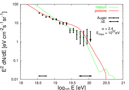
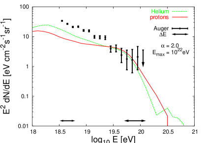
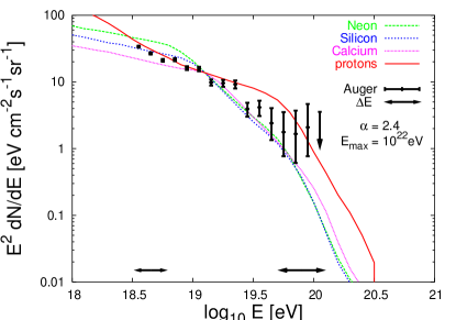
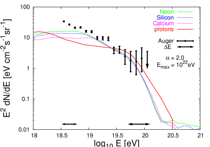
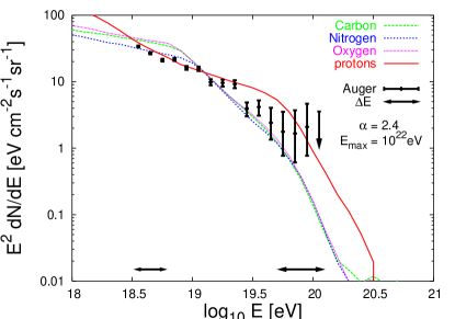
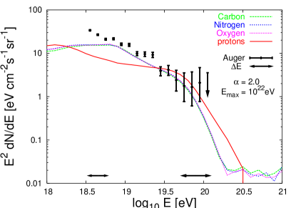
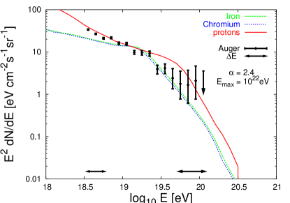
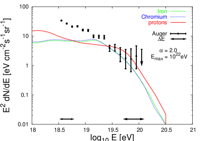
Figure 7: The spectrum of UHECRs observed at Earth for a range of injected heavy nuclei with power-law spectral index $\alpha=2.4$ or 2.0 and $E_{\rm max}=10^{22}$ eV. The overall flux has in each case been normalized to the Auger data Sommers:2005vs . The Malkan & Stecker CIB model Malkan:2000gu and the Lorentzian model Khan:2004nd for photodisintegration cross-sections have been used. The effects of magnetic fields have not been included.

VI The Composition at Earth

If intermediate mass or heavy nuclei are injected in a distant cosmic ray accelerator, these particles will gradually disintegrate into lighter nuclei and nucleons as they propagate through intergalactic space. Depending on the distance to the sources, the cosmic ray composition observed at Earth may be quite different from that at injection.

The observed composition at Earth has a distinctive dependence on the energy as can be seen in Figure 8. In the interesting energy range $\sim 3\times 10^{19}-10^{20}$ eV, i.e. where the GZK suppression is expected for proton primaries, photodisintegration is most effective. For sources injecting intermediate mass nuclei, the effective mass number at Earth reaches a well-defined minimum, probably indistinguishable from proton primaries. This minimum is less pronounced for injection of very heavy nuclei and the effective composition at Earth is distinctly heavier than protons.

These issues are of critical importance, observationally speaking. The injected composition of the UHECR spectrum is not directly accessible experimentally, and can only be reconstructed from the composition observed at Earth. As stated earlier, the present observational status is rather uncertain. Future data will hopefully reach a level of quality which makes it possible to reliably infer the approximate composition at Earth. With such data, general trends such as those seen in Figure 8 would aid in estimating the composition of cosmic rays at the sources.

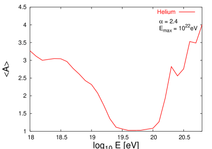
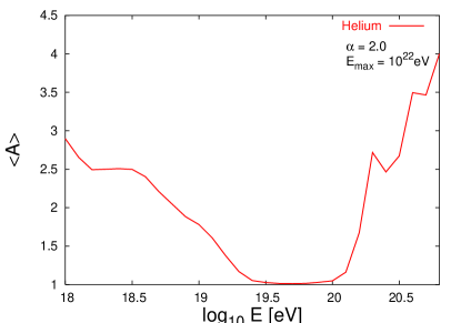
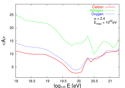
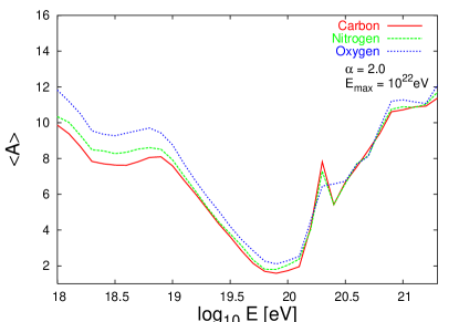
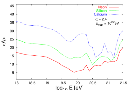
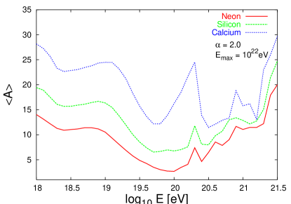
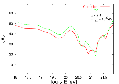
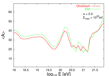
Figure 8: The mean atomic mass of cosmic rays arriving at Earth for a range of injected heavy nuclei with power-law spectral index $\alpha=2.4$ or 2.0 and $E_{\mathrm{max}}=10^{22}$ eV. The Malkan & Stecker CIB model Malkan:2000gu and the Lorentzian model Khan:2004nd for photodisintegration cross-sections have been used. The effects of magnetic fields have not been included.

VII Effects of Intergalactic Magnetic Fields

So far in this study, we have neglected the effects of magnetic fields on the propagation of UHECRs. For protons or nuclear primaries, however, such effects can play an important role in determining the cosmic ray spectrum. The importance of these effects depend, of course, on the strength of the extragalactic magnetic fields which is currently a subject of some debate with contrary conclusions drawn in Ref. Dolag:2004kp and in Refs. Sigl:2003ay ; Armengaud:2004yt .

A charged particle moving through a uniform magnetic field undergoes an angular deflection upon traversing a distance, $L_{\rm{coh}}$, of $\alpha=L_{\rm{coh}}/R_{L}$, where $R_{L}$ is the Larmor radius of the particle. Therefore a particle traversing a distance, $L$, through a series of $L/L_{\rm{coh}}$ randomly orientated uniform magnetic field regions of length $L_{\rm{coh}}$, suffers an overall angular deflection given by

$$\theta(E,Z)\approx\bigg{(}\frac{L}{L_{\rm{coh}}}\bigg{)}^{0.5}\,\alpha\approx 0.8^{\circ}\,\bigg{(}\frac{10^{20}\,\rm{eV}}{E}\bigg{)}\,\bigg{(}\frac{L}{10\,\rm{Mpc}}\bigg{)}^{0.5}\,\bigg{(}\frac{L_{\rm{coh}}}{1\,\rm{Mpc}}\bigg{)}^{0.5}\,\bigg{(}\frac{B}{1\,\rm{nG}}\bigg{)}\,\,Z,$$ (10)

where $L_{\rm{coh}}$ is the representative coherence length of the extragalactic magnetic fields, $B$ is their representative magnitude and $Z$ is the electric charge of the cosmic rays. Such deflections result in an increase in the effective distance to a cosmic ray source given by:

$$\frac{L_{\rm{eff}}}{L}(E,Z)\approx 1+\frac{\theta^{2}}{2}\approx 1+0.065\,\bigg{(}\frac{10^{20}\,\rm{eV}}{E}\bigg{)}^{2}\,\bigg{(}\frac{L}{10\,\rm{Mpc}}\bigg{)}\,\bigg{(}\frac{L_{\rm{coh}}}{1\,\rm{Mpc}}\bigg{)}\,\bigg{(}\frac{B}{1\,\rm{nG}}\bigg{)}^{2}\,\,\bigg{(}\frac{Z}{26}\bigg{)}^{2}.$$ (11)

Thus for protons or light nuclei, nano-Gauss magnetic fields have little impact for the high energies considered here. This is not true for heavy nuclei, e.g. for iron nuclei propagating through nG-scale magnetic fields, the effective distance to a source 50 Mpc away is increased by $\sim 30\%$ at $10^{20}$ eV (alternatively, the energy loss length is reduced by about $\sim 30\%$). Since this effect scales with the inverse square of the cosmic ray energy, such (plausible strength) magnetic fields would have a dramatic effect on the propagation of lower energy heavy nuclei.

In Figure 9 we show the effects of such extragalactic magnetic fields on the UHECR spectrum. For oxygen primaries, the effects are small, only becoming of any consequence at energies below a few times $10^{19}$ eV. However the effects are more prominent for iron primaries.

Some words of caution are called for at this point. The effects of nG-scale magnetic fields appear to set in at an energy of roughly $5\times 10^{19}\,\rm{eV}$ for oxygen, whose primaries can arrive from approximately $300$ Mpc at this energy, corresponding to an effective length of roughly $L_{\rm{eff}}/L\sim 1+0.7\times(B/\rm{nG})^{2}$. This means that the small angle treatment is valid for magnetic fields of strength upto $\sim 0.3$ nG. On the other hand, an iron nucleus with an energy of $5\times 10^{19}$ eV could have traveled hundreds or even thousands of Mpc before its arrival at Earth, so would have been deflected by an angle of $\theta\sim 130^{\circ}\times(L/100\,\rm{Mpc})^{0.5}\times(B/nG)$. Hence the result in the right frame of Figure 9 is not reliable at low energies; to properly take into account such strong deflections, a numerical simulation of diffusion including an appropriate description of the magnetic field structure in the local supercluster is required. Such a treatment is however beyond the scope of the present study.

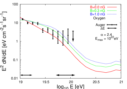
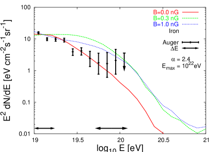
Figure 9: The effects of nano-Gauss extragalactic magnetic fields on the UHECR spectrum for oxygen and iron primaries with power-law spectral index $\alpha$ = 2.4 and $E_{\mathrm{max}}$=10²² eV, assuming $L_{\rm{coh}}\sim$ 1 Mpc. The overall flux has in each case been normalized to the Auger data Sommers:2005vs . The Malkan & Stecker CIB model Malkan:2000gu and the Lorentzian model Khan:2004nd for photodisintegration cross-sections have been used.

VIII Mixed Ultra-High Energy Cosmic Ray Composition

We now study the possibility that a mixture of protons, helium, oxygen, and iron nuclei are injected at source in roughly the same proportions as those observed in low-energy galactic cosmic rays gal . In particularl we will consider a mixture in the ratio of H : He : O : Fe = 1 : 0.85 : 0.06 : 0.02 for a power-law spectral index $\alpha=2.0$, and H : He : O : Fe = 1 : 1.48 : 0.19 : 0.09 for the case of $\alpha=2.4$.

The injection spectrum is assumed to have a cutoff modelled as:

$$\frac{dN}{dE}\propto E^{-\alpha}\exp\bigg{[}{-\bigg{(}\frac{E}{E_{\mathrm{max}}}\bigg{)}\bigg{(}\frac{26}{Z}\bigg{)}\bigg{]}}$$ (12)

with the cutoff energy in the range: $10^{20.5}\,\rm{eV}\,\leq E_{\mathrm{max}}\leq 10^{22}$eV. Once again, the choice of the spectrum is motivated by the possibility that cosmic ray sources can accelerate charged particles to a maximum energy proportional to the charge. This leads to the expectation that such sources will preferentially accelerate heavy nuclei to the highest energies, if such particles are indeed able to survive the radiation fields present in the sources.

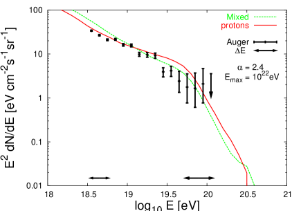
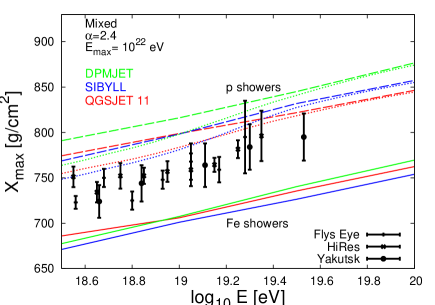
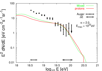
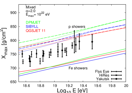
Figure 10: The spectrum (left) and depth of shower maximum, $X_{\mathrm{max}}$, (right) for a mixture of protons, helium, oxygen, and iron injected at source with proportions following that of the Galactic cosmic rays. The solid, dashed, and dotted lines are the predicted values of $X_{\mathrm{max}}$ for, respectively, a pure iron, pure proton, and the mixed composition, obtained using three simulation programmes — DPMJET, SIBYLL and QGSJET. The overall flux has in each case been normalized to the Auger data Sommers:2005vs . The $X_{\mathrm{max}}$ data are from the Fly’s Eye Bird:1993yi , HiRes Abbasi:2004nz and Yakutsk yakutsk experiments. The Malkan & Stecker CIB model Malkan:2000gu and the Lorentzian model Khan:2004nd for photodisintegration cross-sections have been used.

In the left frames of Figure 10, we plot the propagated spectrum calculated using this mixed composition at source, compared to that for pure proton injection. It is seen that the two cases are in fact hard to distinguish observationally.

In the right frames of Figure 10, we plot the average value of $X_{\mathrm{max}}$ as a function of the energy for the same mixed composition at source. To illustrate the uncertainties in relating $X_{\mathrm{max}}$ to the UHECR composition, we have shown the results of three air shower simulation programmes: DPMJET Kalmykov:1997te , SIBYLL sibyll , and QGSJET Kalmykov:1997te . Also shown in Figure 10 are the measurements from the Fly’s Eye Bird:1993yi , HiRes Abbasi:2004nz , and Yakutsk yakutsk experiments. (The $X_{\mathrm{max}}$ values quoted in the Auger analysis which sets an upper bound to the photon content in UHECRs Risse:2005hi are explicitly stated to be inappropriate for elongation rate studies.) The data favour a composition heavier than protons, regardless of which simulation program is adopted.

IX Predictions for $X_{\mathrm{max}}$ Measurements

Information on the UHECR composition at Earth can be obtained from studies of cosmic ray shower development, in particular the lateral distribution, muon content, and $X_{\mathrm{max}}$ value Watson:2004ew . In this Section, we will focus on the parameter $X_{\mathrm{max}}$, which is the atmospheric depth at which the number of particles in the shower is largest. Measurements of $X_{\mathrm{max}}$ are made by fluorescence detector experiments which measure the UV light emitted by the excited atoms (mainly nitrogen) in the air shower.

In the left frames of Figure 11, we show the UHECR spectrum and values of $X_{\mathrm{max}}$ calculated for iron, oxygen and helium nuclei injected at source, with a power-law spectral slope of $\alpha=2.4$ and $E_{\mathrm{max}}=10^{20.5}$ eV. With this rather low choice of the cutoff energy, heavy nuclei dominate the spectrum above $\sim 10^{19}$ eV — iron and oxygen nuclei break up rather modestly during propagation, so the composition at Earth is similar to that at source. In the right frames of Figure 11, we repeat the calculations for the case of $\alpha=2.0$ and find similar results..

For the case of a low cutoff energy, we expect a transition from a heavy composition at high energies to a much lighter composition at low energies, largely independently of the ratio of species present in the source environment. From the spectra shown in Figure 11, we would expect a nearly all-iron composition at the highest energies, and a nearly all proton/helium composition below $\sim 10^{19}$ eV, with the value of $X_{\mathrm{max}}$ changing over this range accordingly. The current data on $X_{\mathrm{max}}$ is too scattered to establish whether such a transition is present.

This conclusion can be modified if the accelerators of UHECRs operate up to a higher cutoff energy so that the heavy nuclei injected at source are substantially photodisintegrated by the time they reach Earth. In Figure 12, we show that for the case $E_{\mathrm{max}}=10^{22}$ eV, it is not at all clear which species will dominant the observed UHECRs — the data is equally well fitted by an all-proton, all-iron or mixed composition at source. What is interesting is that the $X_{\mathrm{max}}$ data is reasonable well fitted when only oxygen nuclei are accelerated by the sources. Even pure iron injection at source matches the data for an injection spectrum with $\alpha=2$.

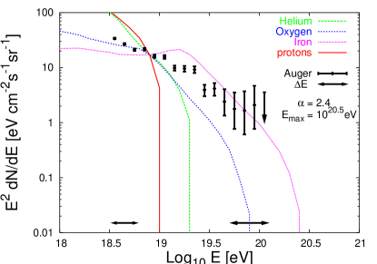
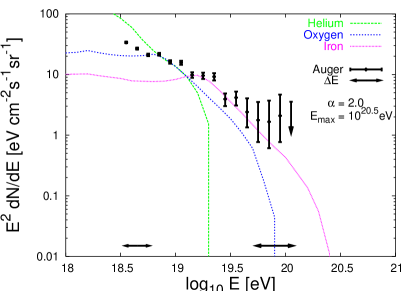
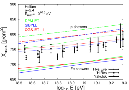
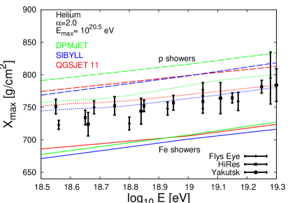
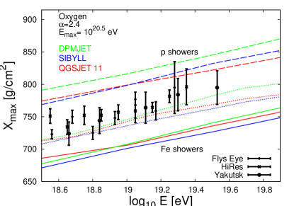
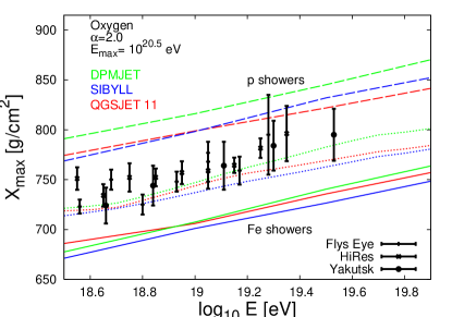
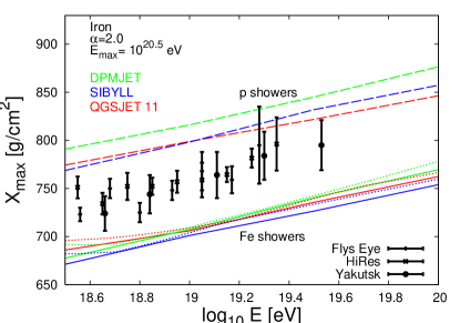
Figure 11: The expected spectrum and X_max for helium, oxygen, and iron nuclei injected at source for E_max=10^20.5eV with $\alpha=2.4$ and 2.0. The overall flux has in each case been normalized to the Auger data Sommers:2005vs . The $X_{\mathrm{max}}$ data are from the Fly’s Eye Bird:1993yi , HiRes Abbasi:2004nz and Yakutsk yakutsk experiments. The Malkan & Stecker CIB model Malkan:2000gu and the Lorentzian model Khan:2004nd for photodisintegration cross-sections have been used.

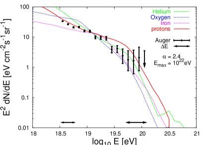
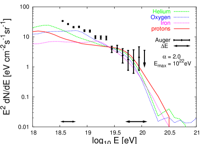
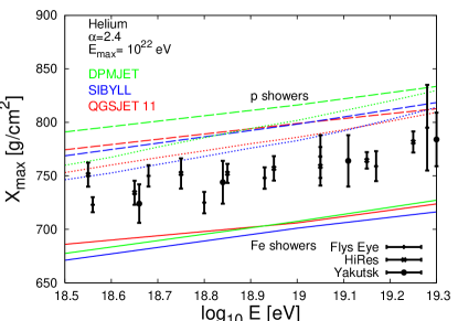
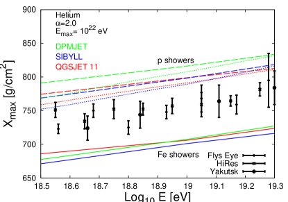
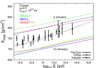
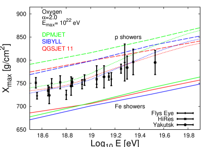
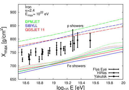
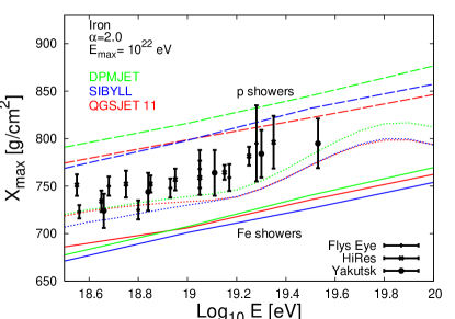
Figure 12: The expected spectrum and X_max for helium, oxygen, and iron nuclei injected at source for E_max=10²²eV with $\alpha=2.4$ and 2.0. The overall flux has in each case been normalized to the Auger data Sommers:2005vs . The $X_{\mathrm{max}}$ data shown are from the Fly’s Eye Bird:1993yi , HiRes Abbasi:2004nz and Yakutsk yakutsk experiments. The Malkan & Stecker CIB model Malkan:2000gu and the Lorentzian model Khan:2004nd for photodisintegration cross-sections have been used.

X Discussion

We have studied the intergalactic propagation of a variety of heavy and intermediate mass cosmic ray nuclei at ultrahigh energies. Adopting different models for the cosmic infrared background and for the photodisintegration cross-sections has little effect on the propagated energy spectrum and composition at Earth. Of more significance is the choice of the source spectrum and the effect of intergalactic magnetic fields. Our main aim was to determine the relationship between cosmic ray composition at source and at Earth after the effects of propagation are taken into account. Somewhat surprisingly, extant data on the composition of UHECRs is consistent with the injection of even pure iron nuclei by the sources.

As the Pierre Auger Observatory continues to accumulate more exposure to UHECRs, a definitive resolution is expected soon of whether there is indeed a GZK cutoff in the spectrum. By combining the energy spectrum obtained using the surface detectors with $X_{\mathrm{max}}$ measurements by the fluorescence telescopes, information can then be extracted on the sources of UHECRs using the results presented in the present paper. Observations of other types of messengers associated with the highest energy cosmic rays, such as the cosmogenic neutrino flux, will also help to determine whether the ultra-high energy cosmic rays are protons or heavy nuclei nu amd bring us closer to answering the long standing mystery of their origin.

- (1) M. Nagano and A. A. Watson, Rev. Mod. Phys. 72 (2000) 689.
- (2) L. Anchordoqui, T. Paul, S. Reucroft and J. Swain, Int. J. Mod. Phys. A 18 (2003) 2229.
- (3) M. A. Lawrence, R. J. O. Reid and A. A. Watson, J. Phys. G 17 (1991) 733.
- (4) D. J. Bird et al., Astrophys. J. 441 (1995) 144.
- (5) M. Takeda et al., Phys. Rev. Lett. 81(1998) 1163.
- (6) T. Abu-Zayyad et al. [HiRes Collab.], Astropart. Phys. 23 (2005) 157.
- (7) K. Dolag, D. Grasso, V. Springel and I. Tkachev, JCAP 0501 (2005) 009.
- (8) K. Greisen, Phys. Rev. Lett. 16 (1966) 748.
- (9) G. T. Zatsepin and V. A. Kuzmin, JETP Lett. 4 (1966) 78.
- (10) P. Sommers [Pierre Auger Collab.], Proc. 29th ICRC, Pune, Vol. 7 (2005) 387.
- (11) V. Berezinsky, M. Kachelriess and A. Vilenkin, Phys. Rev. Lett. 79 (1997) 4302.
- (12) M. Birkel and S. Sarkar, Astropart. Phys. 9 (1998) 297.
- (13) T. J. Weiler, Astropart. Phys. 11 (1999) 303.
- (14) D. Fargion, B. Mele and A. Salis, Astrophys. J. 517 (1999) 725.
- (15) G. Domokos and S. Kovesi-Domokos, Phys. Rev. Lett. 82 (1999) 1366.
- (16) P. Jain, D. W. McKay, S. Panda and J. P. Ralston, Phys. Lett. B 484 (2000) 267.
- (17) I. F. M. Albuquerque, G. R. Farrar and E. W. Kolb, Phys. Rev. D 59 (1999) 015021.
- (18) J. Szabelski, T. Wibig and A. W. Wolfendale, Astropart. Phys. 17 (2002) 125; L. A. Anchordoqui, G. E. Romero and J. A. Combi, Phys. Rev. D 60 (1999) 103001; L. Anchordoqui, H. Goldberg, S. Reucroft and J. Swain, Phys. Rev. D 64 (2001) 123004.
- (19) D. J. Bird et al. [HiRes Collab.], Phys. Rev. Lett. 71 (1993) 3401;
- (20) B. N. Afanasiev (Yakutsk Collab.), Proc. Tokyo Workshop on Techniques for the Study of the Extremely High Energy Cosmic Rays, ed. M. Nagano (1993).
- (21) T. Abu-Zayyad et al. [HiRes-MIA Collab.], Astrophys. J. 557 (2001) 686; M. Ave, L. Cazon, J. A. Hinton, J. Knapp, J. LLoyd-Evans and A. A. Watson, Astropart. Phys. 19 61 (2003) 61.
- (22) A. A. Watson, Nucl. Phys. Proc. Suppl. 151 (2006) 83.
- (23) F. Halzen, R. A. Vazquez, T. Stanev and H. P. Vankov, Astropart. Phys. 3 (1995) 151.
- (24) K. Shinozaki et al., Astrophys. J. 571 (2002) L117.
- (25) M. Ave, J. A. Hinton, R. A. Vazquez, A. A. Watson and E. Zas, Phys. Rev. Lett. 85 (2000) 2244.
- (26) M. Risse [Pierre Auger Collab.], arXiv:astro-ph/0507402.
- (27) J. Knapp, D. Heck, S. J. Sciutto, M. T. Dova and M. Risse, Astropart. Phys. 19 (2003) 77.
- (28) M. T. Dova, M. E. Mancenido, A. G. Mariazzi, T. P. McCauley and A. A. Watson, Astropart. Phys. 21 (2004) 597.
- (29) R. U. Abbasi et al. [HiRes Collab.], Astrophys. J. 622 (2005) 910.
- (30) G. Sigl, F. Miniati and T. A. Ensslin, Phys. Rev. D 68, 043002 (2003).
- (31) A. M. Hillas, Ann. Rev. Astron. Astrophys. 22 (1984) 425.
- (32) L. A. Anchordoqui, M. T. Dova, L. N. Epele and J. D. Swain, Phys. Rev. D 57 (1998) 7103.
- (33) L. N. Epele and E. Roulet, JHEP 9810 (1998) 009.
- (34) F. W. Stecker and M. H. Salamon, Astrophys. J. 512 (1999) 521.
- (35) G. Bertone, C. Isola, M. Lemoine and G. Sigl, Phys. Rev. D 66 (2002) 103003.
- (36) T. Yamamoto, K. Mase, M. Takeda, N. Sakaki and M. Teshima, Astropart. Phys. 20 (2004) 405.
- (37) E. Khan et al., Astropart. Phys. 23 (2005) 191.
- (38) E. Armengaud, G. Sigl and F. Miniati, Phys. Rev. D 72 (2005) 043009.
- (39) D. Allard, E. Parizot, E. Khan, S. Goriely and A. V. Olinto, arXiv:astro-ph/0505566.
- (40) G. Sigl and E. Armengaud, JCAP 0510 (2005) 016.
- (41) D. Allard, E. Parizot and A. V. Olinto, arXiv:astro-ph/0512345.
- (42) G. Blumenthal, Phys. Rev. D 1 (1970) 6.
- (43) A. Mucke, R. Engel, J. P. Rachen, R. J. Protheroe and T. Stanev, Comput. Phys. Commun. 124 (2000) 290.
- (44) We have used the proton-photon cross-section tabulated by the Particle Data Group: http://pdg.lbl.gov/sbl/gammap_total.dat
- (45) T. Stanev, Phys. Lett. B 595 (2004) 50.
- (46) F. W. Stecker, Phys. Rev. 180 (1969) 1264.
- (47) J. L. Puget, F. W. Stecker and J. H. Bredekamp, Astrophys. J. 205 (1976) 638.
- (48) M. A. Malkan and F. W. Stecker, Astrophys. J. 555 (2001) 641.
- (49) F. Aharonian et al. [HEGRA Collab.], Astron. & Astrophys. 403 (2003) 523A.
- (50) A. Franceschini et al., Astron. & Astrophys. 378 (2001) 1F.
- (51) M. G. Hauser and E. Dwek, Ann. Rev. Astron. Astrophys. 39 (2001) 249.
- (52) M. G. Hauser et al., Astrophys. J. 508 (1998) 25.
- (53) L. Metcalfe et al., Astron. Astrophys. 407 (2003) 791.
- (54) P. Madau and L. Pozzetti, Mon. Not. R. Astron. Soc. 312 (2000) L9.
- (55) R. A. Bernstein, W. L. Freedman and B. F. Madore, Astrophys. J. 571 (2002) 56.
- (56) J. P. Gardner, T. M. Brown and H. C. Ferguson, Astrophys. J. 542 (2000) L79.
- (57) T. Matsumoto et al., Lecture Notes in Physics 548 (2000) 96.
- (58) F. Aharonian et al., Nature 440 (2006) 1018.
- (59) J. A. Simpson, Ann. Rev. Nucl. Part. Sci. 33 (1983) 323.
- (60) J. Ranft, Phys. Rev. D 51 (1995) 64
- (61) N. N. Kalmykov, S. S. Ostapchenko and A. I. Pavlov, Nucl. Phys. Proc. Suppl. 52B (1997) 17.
- (62) R. S. Fletcher, T. K. Gaisser, P. Lipari, and T. Stanev, Phys. Rev. D 50 (1994) 5710; J. Engel, T. K. Gaisser, P. Lipari, and T. Stanev, Phys. Rev. D 46 (1992) 5013.
- (63) D. Hooper, A. Taylor and S. Sarkar, Astropart. Phys. 23 (2005) 11; M. Ave, N. Busca, A. V. Olinto, A. A. Watson and T. Yamamoto, Astropart. Phys. 23 (2005) 19; D. Allard et al., arXiv:astro-ph/0605327.