3D Ly$\alpha$ radiation transfer. I. Understanding Ly$\alpha$ line profile morphologies

Abstract

Aims. The development of a general code for 3D Ly$\alpha$ radiation transfer in galaxies to understand the diversity of Ly$\alpha$ line profiles observed in star forming galaxies and related objects.

Methods. Using a Monte Carlo technique we have developed a 3D Ly$\alpha$ radiation transfer code allowing for prescribed arbitrary hydrogen density, ionisation, temperature structures, and dust distributions, and arbitrary velocity fields and UV photon sources.

Results. As a first test and application we have examined the Ly$\alpha$ line profiles predicted for several simple geometrical configurations and their dependence on the main input parameters. Overall, we find line profiles reaching from doubly peaked symmetric emission to symmetric Voigt (absorption) in static configurations with increasing dust content, and asymmetric red- (blue-) shifted emission lines with a blue (red) counterpart ranging from absorption to emission (with increasing line/continuum strength) in expanding (infalling) media. In particular we find the following results which are of interest for the interpretation of Ly$\alpha$ profiles from galaxies. 1) Standard Ly$\alpha$ absorption line fitting of global spectra of galaxies may lead to an underestimate of the true hydrogen column density in certain geometrical conditions. 2) Normal (inverted) P-Cygni like Ly$\alpha$ profiles can be obtained in expanding (infalling) media from objects without any intrinsic Ly$\alpha$ emission, as a natural consequence of radiation transfer effects. 3) The formation and the detailed shape of Ly$\alpha$ profiles resulting from expanding shells has been thoroughly revised. In particular we find that, for sufficiently large column densities ($N_{\rm H}$ $\ga 10^{20}$ cm^-2), the position of the main Ly$\alpha$ emission peak is quite generally redshifted by approximately twice the expansion velocity. This is in excellent agreement with the observations of $z\sim 3$ LBGs, which show that Ly$\alpha$ is redshifted by $\sim 2V_{\rm exp}$, where $V_{\rm exp}$ is the expansion velocity measured from the interstellar absorption lines blueshifted with respect to the stellar redshift. This finding indicates also that large scale, fairly symmetric shell structures must be a good description for the outflows in LBGs.

1 Introduction

The Ly$\alpha$ line plays an important role in a variety of astrophysical problems, especially as a diagnostic tool to observe and study the high redshift universe. It is a simple redshift indicator for distant galaxies, a frequently used star formation rate diagnostic at high $z$, as well as an important tool probing the ionisation state of the intergalactic medium and hence the reionisation epoch. The Ly$\alpha$ emission line is e.g. a strong feature observed in nearby star forming galaxies, distant Lyman break galaxies (LBGs), sub-mm galaxies, emission line selected galaxies (LAE, for Lyman-$\alpha$ emitters), and in the enigmatic so called Lyman-$\alpha$ blobs (LABs) whose nature remains debated (e.g. Steidel et al. 2000, Dijkstra et al.  2005b).

Since the early suggestion of strong Ly$\alpha$ emission from young high redshift galaxies by Partridge & Peebles (1967) and until the late 1990s, only few Ly$\alpha$ emitters have been found (cf. Djorgovski & Thompson 1992). This lack of Ly$\alpha$ emission detection has triggered a variety of studies discussing the possible physical effects (mostly metallicity, dust, neutral gas kinematics, and geometry) which may significantly affect and suppress the Ly$\alpha$ emission and the resonance line radiation transfer, thereby reducing the observed Ly$\alpha$ intensity and destroying simple expected correlations, e.g. between Ly$\alpha$ intensity and metallicity, Ly$\alpha$ intensity and UV continuum flux and others (Meier & Terlevich 1981, Hartmann et al. 1988, Neufeld 1990, Charlot & Fall 1993, Valls-Gabaud 1993, Kunth et al. 1998, Tenorio-Tagle et al. 1999, Mas-Hesse et al. 2003).

In the last few years, with the availability of deeper and wider surveys such as the Large Area Lyman Alpha (LALA) survey and the Subaru Deep Field survey, many emission galaxies have been detected (cf. Hu et al. 1998, 2004; Kudritzki et al. 2000, Rhoads et al. 2000, Ouchi et al. 2003, Taniguchi et al. 2005). Although the majority of these distant Ly$\alpha$ emitters shows rather simple asymmetric line profiles, the overall diversity of the observed Ly$\alpha$ line shapes, both from star forming galaxies in the nearby universe and at high-$z$, is quite heterogeneous and complex. The observed line profiles include schematically pure Voigt absorption profiles, P-Cygni profiles, double peak profiles, pure (symmetric) emission line profiles, and combinations thereof (see e.g. Kunth et al. 1998, Mas-Hesse et al. 2003, Shapley et al. 2003, Möller et al. 2004, Venemans et al. 2005, Wilman et al. 2005, Noll et al. 2004, Tapken et al. 2004, Tapken 2005).

Although in principle the main physical processes shaping the Ly$\alpha$ line are known, in practice the inferences drawn so far from Ly$\alpha$ observations rely mostly on rather simple measurements (e.g. line flux) or on oversimplified Voigt-profile fits, which often have no strong physical motivations. For example, for a Ly$\alpha$ line profile formed purely within a galaxy (i.e. neglecting subsequent alterations from the intergalactic medium and/or intervening clouds), it is physically inconsistent to fit one or several Voigt profiles without making strong implicit assumptions on the geometry of the neutral gas. In such a case, due to the resonance scattering nature of Ly$\alpha$  it is in fact unlikely that the resulting emergent line profile is actually a Voigt profile and a detailed radiation transfer calculation has thus to be carried out to predict the proper shape of the emergent resonance line profile. In general, quantitative simulations for appropriate geometries and gas kinematics, which take properly into account the main physical processes of Ly$\alpha$ line formation and radiation transfer are therefore needed for a better understanding of the variety of observed Ly$\alpha$ line profile morphologies. The physical properties of the Ly$\alpha$ emission mechanism and the ones of the ambient gas hosting the Ly$\alpha$ emitter, which both shape the observed Ly$\alpha$ line, must be properly modeled to investigate the correspondent impact on the emergent line profile and their possible degeneracies. This in turn will provide useful hints to guide the interpretation of the observed profiles and to gain insight on the physical properties of the Ly$\alpha$ emitters and of their environment.

Analytic solutions for the Ly$\alpha$ radiation transfer problem have been derived for simple geometries. Neufeld (1990) has extensively studied the case of static plane parallel slabs, yielding important insight on the line formation mechanism and providing solutions for configuration including dust, Bowen fluorescence and Ly$\alpha$ pumping of H₂ Lyman band lines. The case of a static, uniform sphere has been recently studied by Dijkstra et al. (2005a). Loeb & Rybicky (1999) and Rybicky & Loeb (1999) have derived solutions for Ly$\alpha$ scattering in a Hubble flow. However, more general geometries and velocity fields do not allow for an analytic solution and require alternative approaches.

Over the last few years, several groups have developed new numerical algorithms, mostly based on Monte Carlo techniques (Spaans 1996, Ahn et al. 2001, 2002; 2003, Ahn 2004; Zheng & Miralda-Escudé 2002; Richling et al. 2001; Richling 2003; Kobayashi & Kamaya 2004; Cantalupo et al. 2005; Dijkstra et al. 2005ab; Hansen & Oh 2006; Tasitsiomi 2006). Some of these codes have been specifically designed for and can be reliably applied only to particular configurations: relatively low column densities (Richling et al. 2001; Richling 2003), Hubble flows (Kobayashi & Kamaya 2004), 1D geometry (Ahn et al.), spherically symmetric configurations Dijkstra et al. 2005ab); others are strongly tailored towards cosmological simulations (Cantalupo et al. 2005, Tasitsiomi 2006) and can deal with clumpy/inhomogeneous media (Spaans, 1996; Richling, 2003; Hansen & Oh 2006). In addition, the effect of dust absorption, which is one of the most important factor affecting Ly$\alpha$ transmission, is treated only in some of the codes above.

In any case, none of these studies has attempted to explain systematically the observed variety of Ly$\alpha$ line profile morphologies. Furthermore, none of the above schemes has so far attempted a detailed modeling of individual galaxies, taking into account the available observational constraints, i.e. constraints on the stellar populations, the ionised and neutral interstellar medium, on dust extinction and including their spatial distribution and kinematics. All this lack in the actual theoretical modeling needs to be filled up, in order to extract some information from the huge reservoir contained in the available observational data. With these objectives in mind, and with the main aim of improving our understanding of Ly$\alpha$ in both nearby and distant starburst galaxies, we have developed a general-purpose 3D Ly$\alpha$ radiation transfer code applicable to arbitrary geometries and velocity fields.

In the present paper we provide a description of the code and test its validity against known solutions and results from other codes reported in the literature. Exploring different geometries, dust-free and dusty media, and different input spectra (e.g. line emission, or continuum + line), we examine the resulting line profiles and their dependence on various physical parameters. Our immediate goals are to obtain an overview over the possible Ly$\alpha$ line profile morphologies, and to gain physical insight into the processes governing them. Applications to observed galaxies and other simulations will be presented later.

The remainder of the paper is structured as follows. A description of the radiation transfer code is given in Sect. 2. Tests of the code and results for simple geometrical configurations (slabs, infalling/expanding halos) are presented in Sect. 3. In Sect. 4 we comment on the formation of damped (Voigt) Ly$\alpha$ profiles and related profiles. Spherically expanding dust-free or dusty shells are re-examined in Sect. 5. An overview of the predicted Ly$\alpha$ line profile morphologies and qualitative comparisons with observations is given in Sect. 6. Our main conclusion are summarised in Sect. 7.

2 Radiation transfer code

A general 3D radiation transfer code MCLya allowing for arbitrary hydrogen density, ionisation & temperature structures, dust distributions, and velocity fields was developed using a Monte Carlo technique. The input files and the structure of the code have been designed for a future joint use with the 3D radiation transfer and photoionisation code CRASH of Maselli et al. (2003). We now summarise the main ingredients and assumptions made in this code.

2.1 Geometry

The present version of the code assumes a 3D cartesian grid of $n^{3}$ cells. Typically we adopt $n=128$. The relevant quantities describing a 3D structure are the neutral hydrogen density distribution, the dust density distribution, the temperature distribution, and the velocity field. These are prescribed by input files.

2.2 Photon sources

Ly$\alpha$ and/or continuum photons are emitted from one or several point sources. Each source is described by :

• its location,

• the total number of emitted photons

• optionally their emission direction, if not isotropic,

• the source spectrum (typically monochromatic, a constant photon density per frequency or wavelength interval, a Gaussian, or combinations thereof).

2.3 Physical processes

To capture the essentials of radiation transfer in the UV including and around the Ly$\alpha$ line we include three main physical processes, dust absorption and scattering and the Ly$\alpha$ line transfer, in the present version of our code. Given the principles of Monte Carlo simulations, other processes can easily be included in the future, if desirable.

2.3.1 Ly$\alpha$ line transfer

In the whole section, we describe the Ly$\alpha$ radiative transfer equations in a static medium. To adapt them to moving media, we just convert frequencies to local co-moving frequencies and convert them back to the external frame by a Lorentz transformation, neglecting terms of order $O(v^{2}/c^{2})$.

A Ly$\alpha$ photon corresponds to the transition between the $n=2$ and $n=1$ levels of a hydrogen atom. This is the strongest H i transition, with an Einstein coefficient given by $A_{21}=6.265\times 10^{8}$ s^-1. The scattering cross-section of a Ly$\alpha$ photon as a function of frequency in the rest frame of the hydrogen atom is:

$$\sigma_{\nu}=f_{12}\,\frac{\pi\,e^{2}}{m_{e}\,c}\,\frac{\Gamma/4\,\pi^{2}}{(\nu-\nu_{0})^{2}+(\Gamma/4\,\pi)^{2}},$$ (1)

where $f_{12}=0.4162$ is the Ly$\alpha$ oscillator strength, $\nu_{0}=2.466\times 10^{15}$ Hz is the line center frequency, and $\Gamma=A_{12}$ is the damping constant which measures the natural line width.

The optical depth $\tau_{\nu}(s)$ of a photon with frequency $\nu$ traveling a path of length $s$ is determined by convolving the above cross-section with the velocity distribution characteristic of the absorbing gas, and is of the form:

$$\tau_{\nu}(s)=\int_{0}^{s}\int_{-\infty}^{\infty}n(V_{z})\,\sigma_{\nu}\,dV_{z}\,dl,$$ (2)

where $V_{z}$ denotes the velocity component along the photon’s direction. Thermal motions of Hydrogen are described by a Maxwellian distribution of atoms velocities whose velocity dispersion, $V_{th}=(2\,k_{B}\,T/m_{\rm{H}})^{1/2}=12.85T_{4}^{1/2}$ km s^-1, corresponds to the Doppler frequency width $\Delta\nu_{D}=(V_{th}/c)\nu_{0}$. Here $T_{4}$ is the gas temperature in units of $10^{4}$ K. In certain cases an additional turbulent motion, characterised by $V_{\rm turb}$, is taken into account in the Doppler parameter $b$ given by

$$b=\sqrt{V_{th}^{2}+V_{turb}^{2}}.$$ (3)

Let us now introduce some useful variables. First the frequency shift in Doppler units

$$x=\frac{\nu-\nu_{0}}{\Delta\nu_{D}}=\frac{V}{b},$$ (4)

where the second equation gives the relation between $x$ and a macroscopic velocity component $V$ measured along the photon propagation (i.e. parallel to the light path and in the same direction). Second the Voigt parameter $a\equiv\frac{\Gamma/4\,\pi}{\Delta\nu_{D}}=4.7\times 10^{-4}\,T_{4}^{-1/2}$, or more generally $a=4.7\times 10^{-4}\,(12.85\,{\rm km\,s^{-1}}/b)$ for non-zero turbulent velocity. Adopting this notation, it can be shown that:

$$\tau_{x}(s)=\sigma_{H}(x)\,n_{H}\,s=1.041\times 10^{-13}\,T_{4}^{\phantom{4}-1/2}\,N_{H}\,\frac{H(x,a)}{\sqrt{\pi}}$$ (5)

where $n_{H}$ is the neutral hydrogen density, and $N_{H}$ the corresponding column density. The Hjerting function $H(x,a)$ describes the Voigt absorption profile,

$$H(x,a)=\frac{a}{\pi}\int_{-\infty}^{\infty}\frac{e^{-y^{2}}dy}{(y-x)^{2}+a^{2}}\approx\left\{\begin{array}[]{ll}e^{-x^{2}}&\textrm{if $|x|<x_{c}$}\\ \frac{a}{\sqrt{\pi}x^{2}}&\textrm{if $|x|>x_{c}$}\end{array}\right.$$ (6)

which is often approximated by a central resonant core and power-law “damping wings” for frequencies below/above a certain boundary frequency $x_{c}$ between core and wings. For $a$ in the range of $10^{-2}$ to $10^{-6}$, $x_{c}$ varies typically from 2.5 to 4. To evaluate $H$ in our code, we use the fit formulae given by Gray (1992).

To characterise the depth of a static medium we will use $\tau_{0}$, the optical depth at line center:

$$\tau_{0}(s) = 1.041\times 10^{-13}\,T_{4}^{-1/2}\,N_{H}\,\frac{H(0,a)}{\sqrt{\pi}}$$ (7)

$$\approx 3.31\times 10^{-14}\,T_{4}^{-1/2}\,N_{H}$$ (8)

for zero turbulent velocity, or more generally

$$\tau_{0}(s)=3.31\times 10^{-14}\,(12.85\,{\rm km\,s^{-1}}/b)\,N_{H}$$ (9)

This monochromatic optical depth $\tau_{0}$ has been used in most recent studies (e.g. Ahn et al. 2001, 2002; Zheng & Miralda-Escudé 2002, Hansen & Oh 2006); however, it differs from the total Ly$\alpha$ optical depth $\tau_{0}^{\rm Neuf}$ used in the classical work of Neufeld (1990) by $\tau_{0}^{\rm Neuf}=\tau_{0}\sqrt{\pi}$.

Once the absorption probability is given and before the Ly$\alpha$ photon is re-emitted, its frequency and angular distribution must be determined. If the atom is not perturbed by collisions during the time a Ly$\alpha$ photon is absorbed and re-emitted, the frequencies before and after scattering are identical in the atom’s rest-frame. On the other hand, when the atom undergo a collision, the electron is reshuffled on another energy level and the frequencies before and after scattering are uncorrelated. Given the typically low densities in astrophysical media, we assume coherent scattering in our code.

Concerning the angular redistribution, our code can model the case of isotropic as well as the more realistic dipolar redistribution. In the case of isotropy, for simplicity and speed we use the angle averaged frequency redistribution function $R_{II-A}(x_{\rm in},x_{\rm out})$ from Hummer(1962). In practice we use pretabulated values of the cumulative frequency distribution function of $R_{II-A}$ for different input frequencies and temperatures. In all the static geometries presented in this paper, we use an isotropic angular redistribution. As test calculations confirm (cf. Fig 1 and also Zheng & Miralda-Escudé 2002 and Hansen & Oh 2006) this is an excellent approximation since the Ly$\alpha$ photons undergo a very large number of scatterings where any angular preference is smeared out.

To avoid numerous core scatterings in static cases with a high column density, different acceleration methods have been developed in other radiation transfer codes (e.g. Ahn & Lee 2002, Djikstra & Haiman 2005a). In our case, such an acceleration is easily included in the redistribution functions by setting artificially $R_{II-A}(x_{\rm in},x_{\rm out})=\epsilon$ where $\epsilon$ is close to zero for $|x_{\rm in}|<x_{c}$ and $|x_{\rm out}|<x_{c}$, which corresponds to setting the probability to be re-emitted at $|x_{\rm out}|<x_{c}$ to zero, when photons are absorbed in the core (i.e. when $|x_{\rm in}|<x_{c}$). In practice we have not used the acceleration method except for test cases, as it turns out that all cases shown here are tractable without it.

The dipolar angular redistribution has been implemented without the use of redistribution functions, but microscopically, following the detailed descriptions of former codes (cf. Zheng & Miralda-Escudé 2002 and Dijkstra & Haiman 2005a). The necessity to use this more physical redistribution is particularly important for expanding shells (see section 5).

2.3.2 Dust scattering and absorption

During its travel in an astrophysical medium, the Ly$\alpha$ photon will diffuse on H atoms, but it can also interact with dust: it can either be scattered, or absorbed. The dust cross-section $\sigma_{d}$ is composed of an absorption cross-section $\sigma_{a}$, and a scattering cross-section $\sigma_{s}$:

$$\sigma_{d}=\sigma_{a}+\sigma_{s}$$ (10)

where $\sigma_{a,s}=\pi\,d^{2}\,Q_{a,s}$, with $d$ the typical dust grain size which will affect Ly$\alpha$ photons, and $Q_{a,s}$ the absorption/scattering efficiency. At UV wavelengths the two processes are equally likely, $Q_{a}\approx Q_{s}\approx 1$, so the dust albedo $A=Q_{s}/(Q_{a}+Q_{s})$ is around 0.5: half of the photons interacting with dust will be lost, and half will be re-emitted in the Ly$\alpha$ line.

We assume that the dust density $n_{d}$ is proportional to the neutral H density in each cell

$$n_{d}=n_{H}\times\frac{m_{\rm{H}}}{m_{d}}\,\frac{M_{d}}{M_{\rm{H}}},$$ (11)

where $m_{d}$ is the grain mass and $m_{\rm{H}}$ the proton mass. The relevant quantity, $\tau_{d}$ given just below, is described by one free parameter, the dust to gas ratio $\frac{M_{d}}{M_{\rm{H}}}$ assuming $d=10^{-6}$ cm and $m_{d}=3\times 10^{-17}$ g. The total (absorption + scattering) dust optical depth seen by a Ly$\alpha$ photon is then:

$$\tau_{d}=\tau_{a}+\tau_{s}=\int_{0}^{s}\sigma_{d}\,n_{d}(s)\,ds.$$ (12)

The relation between the dust absorption optical depth at Ly$\alpha$ wavelength $\tau_{a}=(1-A)\tau_{d}$ and the color excess $E_{B-V}$ is given by

$$E_{B-V}=1.086\frac{A_{V}}{A_{1216}\,R}\,\tau_{a}\approx(0.06\ldots 0.11)\,\tau_{a}$$ (13)

where $A_{V}$ and $A_{1216}$ is the extinction in the $V$ band and at 1216 Å respectively, $R$ the total-to-selective extinction. The smaller numerical value corresponds to a Calzetti et al. (2000) attenuation law for starbursts, the larger to the Galactic extinction law from Seaton (1979).

2.4 Monte Carlo radiation transfer

For each photon source we emit photons one by one, and we follow each photon until escape from our simulation box or absorption by dust. Let us now describe one photon’s travel.

2.4.1 Initial emission

The emission of a photon is characterised by an emission frequency and direction. The frequency $\nu$ (here in the “external”, i.e. observer’s frame) samples the source spectrum representing usually Ly$\alpha$ line emission and/or UV continuum photons. For media with constant temperature, $\nu$ or more precisely the emission frequency shift from the line center, is conveniently expressed in Dopper units, i.e. $x=(\nu-\nu_{0})/\Delta\nu_{D}$ (cf. Eq. 4).

We assume that the source emission is isotropic (in the local co-moving frame, if the considered geometry is not static). Thus the emission direction, described by the two angles $\theta$ and $\phi$, is randomly selected from

$$\theta = cos^{-1}(2\,\xi_{1}-1)$$ (14)

$$\phi = 2\,\pi\,\xi_{2}$$ (15)

where $\xi_{1,2}$ are random numbers , $0\leq\xi_{1,2}<1$. The photon travels in this direction until it undergoes an interaction. In moving media, the photon frequency in the external frame is evaluated by a Lorentz transformation.

2.4.2 Location of interaction

The location of interaction is determined as follows. The optical depth, $\tau_{int}$, that the photon will travel is determined by sampling the interaction probability distribution $P(\tau)=1-e^{-\tau}$ by setting

$$\tau_{int}=-ln(1-\xi)$$ (16)

where $\xi$ is another random number.

We sum the optical depth $\tau$ along the photon path $s$:

$$\tau(s)=\tau_{x}(s)+\tau_{d}(s)$$ (17)

and we determine the length $s$ corresponding to $\tau(s)=\tau_{int}$. We calculate the coordinates corresponding to a travel of length $s$ in the direction ($\theta,\phi$) starting from the emission point. This is the location of interaction. Now, we have to compute if the Ly$\alpha$ photon interacts with a dust grain or a hydrogen atom.

2.4.3 Interaction with H or Dust ?

The probability to be scattered by a hydrogen atom is given by:

$$P_{\rm{H}}(x)=\frac{n_{H}\sigma_{H}(x)}{n_{H}\sigma_{\rm{H}}(x)+n_{d}\sigma_{d}},$$ (18)

where $\sigma_{\rm{H}}(x)=f_{12}\,\frac{\pi\,e^{2}}{m_{e}\,c\,\Delta\nu_{D}}\,H(x,a)$ is the hydrogen cross section for a Ly$\alpha$ photon of frequency $x$. We generate a random number $0\leq\xi<1$ and compare it to $P_{\rm{H}}$: if $\xi\,<\,P_{\rm{H}}$, the photon interacts with H, otherwise it is scattered or absorbed by dust.

2.4.4 Scattering on H atoms

When the photon is absorbed by an H atom, how will it be reemitted ?

We first convert the frequency in the external (observers) frame, $\nu_{ext}$, to the comoving frequency of the fluid, $\nu_{int}$, with a Lorentz transformation

$$\nu_{int}=\nu_{ext}(1-\frac{\@vec{k}_{i}\cdot\@vec{V}}{c}),$$ (19)

where $\@vec{k}_{i}$ is the photon direction and $\@vec{V}$ the macroscopic/bulk velocity of the H atoms. As already mentioned above, we assume partially coherent scattering and either isotropic or dipolar angular redistribution. After scattering, the new frequency is again converted back to the external frame.

2.4.5 Dust scattering and absorption

When the photon interacts with dust, we generate a random number $0\leq\xi<1$ determining whether it is absorbed or scattered. In practice, if $\xi<A=Q_{s}/(Q_{a}+Q_{s})$ the photon is scattered by dust and simply reemitted coherently. Otherwise the photon is absorbed by dust and is considered lost for the present simulation. For the same reasons already discussed above (Sect. 2.3.1) we currently assume that dust scattering is isotropic, but other angular distributions (e.g. Henyey-Greenstein functions) can easily be implemented.

2.4.6 Output

The precedent scheme is repeated until the photon escapes the simulation volume, or undergoes a dust absorption. Then, we store all the information concerning this photon in a matrix and start with the next photon. This procedure is repeated for all photons and all emission sources. Finally all the desired results, such as spatially integrated line profiles, monochromatic or integrated Ly$\alpha$ images, surface brightness contours for any given line of sight and spatial resolution etc. are computed from this output matrix. For reasons of symmetry, and to maximise the numerical efficiency, all the spectra presented hereafter are integrated spectra over all directions, except if mentioned otherwise (cf Fig 11).

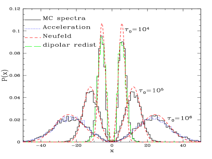
Figure 1: Predicted emergent Ly$\alpha$ profiles for monochromatic line radiation emitted in a dust-free slab of different optical depths (solid lines) compared with analytic solutions from Neufeld (1990, dashed). The dotted blue curve shows the line profile obtained using a frequency redistribution function, which skips a large number of resonant core scatterings. The adopted conditions of the medium are: $T=10$ K (i.e. $a=1.5\,10^{-2}$), and $\tau_{0}=10^{4}$, $10^{5}$, $10^{6}$ from top to bottom. The green long-dashed curve, obtained with a dipolar angular redistribution, overlaps perfectly the black solid line, obtained with the isotropic angular redistribution function, illustrating the fact that in static media, isotropy is a very good approximation.

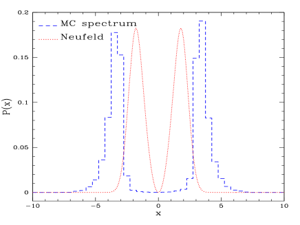
Figure 2: Same as Fig. 1 for a slab of small optical depth ($\tau_{0}=10^{4}$) and high temperature $T=10^{4}$ K ($a=4.7\,10^{-4}$) illustrating the deviation from the analytic solution of Neufeld (1990) due to the more complete treatment of the line absorption profile (see text).

3 Validation of the code and examination of simple geometrical configurations

To validate/test our code and to gain insight into basic properties of the Ly$\alpha$ radiation transfer we have computed a large number of simulations for geometrical setups discussed previously in the literature : slabs, expanding/infalling halos, expanding shells that we will present in details hereafter, and disk-like configurations for which we have perfect agreement with Richling et al. (2003).

We consider various input spectra (i.e. the intrinsic emission line profile and possible continuum emission), especially the limiting cases of a pure monochromatic (i.e. line) radiation. Both cases with or without dust are considered. The case of a source emitting a pure continuum in a plane parallel slab with and without dust is discussed in Sect. 4.

3.1 Homogeneous slab

The best studied case is that of a plane parallel homogeneous slab, for which analytic solutions of the Ly$\alpha$ transfer problem have been derived and discussed in depth by Neufeld (1990). For a given source position and input spectrum, the main physical quantities determining the output spectrum are the temperature of the medium and its optical depth, whatever the angular redistribution is. Note that in this section, all profiles have been obtained using isotropic angular redistribution, except if the contrary is specified.

3.1.1 Monochromatic radiation, no dust

As a first test we simulate a dust-free slab with a central plane source emitting Ly$\alpha$ photons in the line center (i.e. $\nu_{0}=2.46\times 10^{15}$ Hz or equivalently $x=0$). We choose $T=10$ K (i.e. $a=1.5\times 10^{-2}$), and vary the optical depth in the line center, $\tau_{0}=10^{4},\,10^{5},\,10^{6}$, to be in the validity range of Neufeld’s analytic solution assuming a power-law absorption profile (Eq. 6): a very optically thick slab, where $a\,\tau_{0}\,>(a\,\tau_{0})_{\rm crit}$ (cf. below). In this case the emergent Ly$\alpha$ line profile is given by (see Neufeld 1990, Eq. 2.24):

$$J(\tau_{0},x)=\frac{\sqrt{6}}{24\sqrt{\pi}}\frac{x^{2}}{a\tau_{0}}\frac{1}{\cosh[\sqrt{\pi^{3}/54}(|x^{3}|/a\tau_{0})]}.$$ (20)

As shown in Fig. 1, our spectra are in perfect agreement with Neufeld’s predictions. The spectra are double peaked and symmetric around $x=0$. The peak frequency $x_{p}$ reflects the physical properties of the neutral medium

$$x_{p}\approx\pm\,0.88(a\,\tau_{0})^{1/3}.$$ (21)

As expected, the more optically thick the medium is, the more separated are the peaks. The width of the peaks becomes larger with larger $\tau_{0}$. In Fig. 1 we also show that computations using our acceleration method (cf. Sect. 2.3.1) yield excellent agreement.

For higher temperature, i.e. smaller $a$ (see Fig. 2) our spectrum differs from the analytic solution of Neufeld (1990), as also noticed by Ahn et al. (2001) and Zheng & Miralda-Escudé (2002). This is due to the simplified assumption of a power-law line profile in the wings, which Neufeld (1990) assumes to be valid for the entire absorption line profile $H$ (cf. Sect. 2.3.1). As a consequence our peaks are more separated and less symmetric than expected from Neufeld’s calculation. This is due to the fact that Neufeld’s approximation of $H$ underestimates the absorption probability in the core, such that photons escape more easily than in the real case and their mean escape frequency remains closer to the line center.

For Neufeld’s analytical solution, based on the assumption that $H(x,a)\approx\frac{a}{\sqrt{\pi}x^{2}}$ as in Lorentz wings, to be valid, a minimum criterium is that the optical depth at the frequency $x_{c}$ corresponding to the transition between core and wings is larger than $1$. Otherwise, most of the Ly$\alpha$ photons will escape from the core where Neufeld’s approximation is not valid. In practice, since $\tau_{\rm crit}=\tau(x_{c})=1$ corresponds to $(a\tau_{0})_{\rm crit}=\sqrt{\pi}x_{c}^{2}$, the analytic solutions of Neufeld (1990) are valid only for sufficiently large optical depths, i.e. for $a\,\tau_{0}\,>(a\,\tau_{0})_{\rm crit}$.

3.1.2 Monochromatic radiation and dust

We now include dust in the slab and examine its effect on line profiles and on Ly$\alpha$ photon destruction.

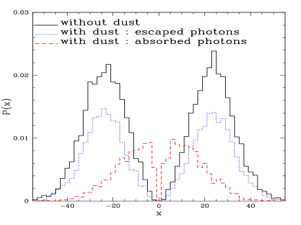
Figure 3: Predicted emergent Ly$\alpha$ profiles for monochromatic line radiation emitted in a slab of optical depth $\tau_{0}=10^{6}$, $T=10$ K, and $\tau_{a}=10^{-3}$ and 0. The black solid line shows the emergent profile without dust and the blue dotted line the one with dust. The red dashed line shows the (unobservable) spectrum of the photons which have been absorbed by dust. The effect of dust seems “grey” on the emergent line profile because $\tau_{\rm dust}$ is very weak. For greater $\tau_{\rm dust}$, the inner part of the peaks is destroyed.

As illustrated in Fig 3, the presence of dust absorption reduces the total Ly$\alpha$ intensity. For the case of monochromatic radiation with a very small amount of dust shown here, the shape of the emerging Ly$\alpha$ profile remains basically unchanged by dust. However, with increasing $\tau_{\rm dust}$, the inner parts of the emission peaks are destroyed. Although not an observable, we also plot the spectrum of the absorbed photons (red dotted line on Fig 3). As expected, it is symmetric with respect to the line center: it presents two peaks, closer to the line center than those of the emerging profile. To understand these features, we have to take into account two competing effects, the large number of scatterings photons undergo in the line core favouring a potential interaction with dust, but the low probability to interact with dust in presence of the very strong HI absorption cross section close to the line core. Indeed, the probability to interact with H is around unity in the core since

$$P_{\rm{H}}(x=0)=\frac{\sigma_{\rm{H}}(0)}{\sigma_{\rm{H}}(0)+\frac{m_{\rm H}}{n_{d}}\frac{M_{d}}{M_{\rm H}}\sigma_{d}}\approx\left[1+c^{\prime}\,T_{4}^{1/2}\frac{M_{d}}{M_{\rm H}}\right]^{-1},$$ (22)

with $c^{\prime}=3.3\,10^{-6}$ K^-1/2 for the dust parameters adopted here. Therefore none of the photons are absorbed by dust in the very center of the line. The peaks are located where the probability to interact with H is lower (for $|x|<x_{c}$) but where the number of interactions (which ultimately increase the chances for dust absorption or scattering) is still high, i.e. on both sides of the line core.

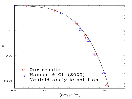
Figure 4: Escape fraction $f_{e}$ for Ly$\alpha$ line photons emitted monochromatically in a dusty slab as a function of $(a\tau_{0})^{1/3}\tau_{a}$. The excellent agreement between our simulation (crosses), the computations of Hansen & Oh (2006) and the approximate analytical solution of Neufeld (1990) given by Eq. 23 is shown.

For an optically thick slab ($a\tau_{0}>10^{3}$), Neufeld (1990) gave an analytic solution to determine the escape fraction, i.e. the ratio between the number of photons which escape the medium and the total number of emitted photons. This escape fraction $f_{e}$ depends on the combination $(a\tau_{0})^{1/3}\tau_{a}$, where $\tau_{a}$ is the optical depth of absorption from the center to the surface of the slab, i.e. $\tau_{a}=\tau_{d}/2$ here since we consider a dust albedo $A\sim 0.5$. For a central source and in the limit $(a\tau_{0})^{1/3}\gg\tau_{a}$, Neufeld (1990, his Eq. 4.43) has derived an approximate expression for $f_{e}$, which, in our notation, is

$$f_{e}=1/\cosh\left[\frac{\sqrt{3}}{\pi^{5/12}\zeta}\left[(a\tau_{0})^{1/3}\tau_{a}\right]^{1/2}\right]$$ (23)

where $\zeta\approx 0.525$ is a fitting parameter. In Fig. 4, we compare our results with this analytical curve and with the results from Monte-Carlo simulations of Hansen & Oh (2006). Our results are in good agreement with both of them.

3.1.3 Continuous input spectrum

The case of a source emitting a pure continuum in a plane parallel slab with and without dust is discussed in Sect. 4.

3.2 Expanding/infalling halos

We now simulate spherical clouds (“halos”) of uniform density, not only static, but also expanding or collapsing. An isotropic Ly$\alpha$ source is either located at the center of the sphere, or uniformly distributed over the whole volume. In this section, the angular redistribution considered is isotropic, after verification that the emergent profiles are very similar, even in the cases with motion.

3.2.1 Monochromatic source

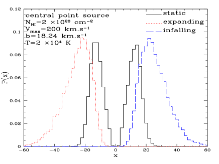
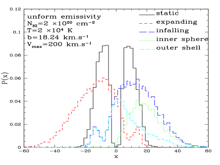
Figure 5: Predicted Ly$\alpha$ profiles of an isotropic and monochromatic source in uniform and isothermal spherical halos with a center to edge column density of $N_{H}=2.\,10^{20}$ cm^-2 and $T=20000$ K (i.e. $b=18.24$ km s^-1). Black solid lines show the Ly$\alpha$ profiles for a static halo, red short-dashed lines the expanding case with $V_{\rm max}=200$ km s^-1, and blue long-dashed the infall case (same $V_{\rm max}$). Left: Central point source. Right: Uniform emissivity. On the right panel, the “infalling” spectrum has been decomposed in two components: the emergent spectrum from an “inner part” (the inner 50 % of the volume), resembling that from a halo with a central source, and the one from the “external part” akin to the spectrum from an expanding shell where photons do not undergo backscatterings (cf. Fig. 12).

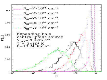
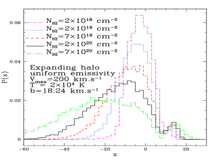
Figure 6: Predicted Ly$\alpha$ profiles of an isotropic and monochromatic source in uniform and isothermal spherically expanding halos with varying column density ($N_{\rm H}=2.\,10^{18}$ to $7.\,10^{20}$ cm^-2 as indicated in the Figure), and other parameters fixed to $T=20000$ K (i.e. $b=18.24$ km s^-1) and $V_{\rm max}=200$ km s^-1. Left: Central point source. Right: Uniform emissivity.

We first chose the same physical conditions as Zheng & Miralda-Escude (2002) and performed a run with a colunm density measured from the center to the edge of the cloud $N_{\rm H}=2.\,10^{20}$ cm^-2, corresponding to a line-center optical depth $\tau_{0}=8.3\,10^{6}$ and a temperature of $2.\,10^{4}$ K. The velocity field is a Hubble-type flow, $V(r)=\pm V_{\rm max}r/R_{\rm max}$, with $V_{\rm max}=200$ km s^-1 at the outer radius $R_{\rm max}$ of the halo, and the positive (negative) sign corresponding to the expanding (infalling) halo. Our results, shown in Fig. 5, are in good agreement with those of Zheng & Miralda-Escude (2002). For static halos, the same characteristic double peak profile as for the static slab (cf. Fig. 1) are obtained both for a uniform emissivity or for a central point source. As shown by Djikstra & Haiman (2005a) the position of the peaks shows the same dependence as for the static slab (Eq. 21), but is given by $x_{p}=\pm 1.06(a\tau_{0})^{1/3}$ for $a\tau_{0}>10^{3}$.

Ly$\alpha$ line profiles from an expanding or infalling halo are perfectly symmetric to each other (compare the red short-dashed and blue long-dashed curves on Fig. 5). Expanding halos present a red peak, whereas infalling halos have a blue one. Halos with a uniform emissivity (right panel in Fig. 5) show 1) broader lines, 2) emission extending on both sides, and 3) a secondary peak on the blue (red) side for the expanding (infalling) halo. The last feature is not visible on the plots of Zheng & Miralda-Escude (2002), but their resolution may be too low. However, the results of Dijkstra & Haiman (2005a) show this secondary peak. We now briefly discuss the origin of these features.

Why are single peaks formed in expanding/infalling media with a central point source emitting monochromatic radiation at the Ly$\alpha$ line center? The reason is simple. The probability to escape the medium for a photon at line center is $e^{-\tau_{0}}$, i.e. close to zero for both cases shown here. As an expanding halo contains atoms with velocities $v(r)$ from 0 to $V_{\rm max}$, all photons in the frequency range $x=[0,V_{\rm max}/b\sim 11]$ will be seen in the line center by atoms of the corresponding velocity, and are thus “blocked”. Therefore the only possibility to escape is to be shifted to the red side. The symmetry of the double peak profile of the static case is “broken” in this way and transformed to a red peak for an expanding halo.

The increased line width in case of a spatially uniform emissivity (1) and the presence of photons on both the red and blue sides (2) is due to the fact that the intrinsic line emission (assumed at $x=0$ in the atom’s frame) spreads already over all frequencies from $x=-V_{\rm max}/b$ to $+V_{\rm max}/b$ in the external (observer’s) restframe. Radiation transfer effects further redistribute the photons in the wings. In fact, for the expanding halo, photons emerging with $x>V_{\rm max}/b$ (i.e. very blue ones) correspond to photons emitted close to the halo edge on the approaching side, which have been further redshifted by diffusion away from the line center (at $x\sim+V_{\rm max}/b$ in the observers frame). This naturally also produces the local minimum observed at this frequency, which separates the secondary peak from the main one (point 3 above). This is easily verified by plotting e.g. the contributions from photons emitted in the “external” parts (i.e. close to the edge) and from “internal”regions, as shown in the right panel of Fig. 5. We chose as inner/outer limit the radius which corresponds to an inner sphere and an outer shell of same volume. Therefore the location of this minimum is a measure of the external velocity of the halo, as already noticed by Dijkstra & Haiman (2005a), at least for velocities $V_{\rm max}\la$ 360 km s^-1 beyond which the two peaks start to overlap.

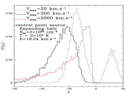
Figure 7: Predicted Ly$\alpha$ profiles from an expanding halo with a central monochromatic source and varying velocity gradients ($V_{\rm max}=$ 20, 200, and 2000 km s^-1) for $T=20000$ K (i.e. $b=18.24$ km s^-1) and $N_{\rm H}=2.\,10^{20}$ cm^-2.

With Figs. 6 and 7, we investigate how the emergent lines depend on column density and velocity gradient. When $N_{\rm H}$ increases, the emission peak is shifted away from line center and broadens out for both cases (central point source and uniform emissivity). Indeed, the optical depth at line center increases with $N_{\rm H}$, so Ly$\alpha$ photons have to diffuse far in the wings to escape. From the right panel of Fig. 6 we note that the location of the flux minimum between the two peaks remains constant quite independently of $N_{\rm H}$. The behaviour for different velocity gradients, first discussed by Wehrse & Peraiah (1979),is the following (cf. Fig. 7): from $V_{\rm max}=20$ to 200 km s^-1 one goes from a nearly static case (i.e. double peaks) to a broad asymmetric line, whose peak position is progressively displaced redwards. Above a certain value of the velocity gradient (or equivalently $V_{\rm max}$), the peak position moves back closer to line center as the medium becomes more “transparent” there, given the finite and constant column density. In any case, the extent of the red wing continues to increase with increasing $V_{\rm max}$. Qualitatively the simulations shown in Figs.  6 and 7 resemble those of a cosmological Hubble flow (cf. Loeb & Rybicky 1999) although modified by a finite outer boundary.

For test purposes we have also compared the surface brightness profiles with the results of Zheng & Miralda-Escude (2002), and find a good agreement.

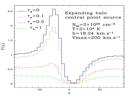
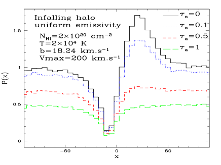
Figure 8: Left: Line profiles for an expanding halo with a central monochromatic source showing the variety of profiles from P-Cygni to somewhat asymmetric damped profiles. Right: Infalling halo with a uniformly distributed emissivity showing profiles from inverted P-Cygni to less broad absorption. In both panels the adopted conditions are the following: $N_{H}=2.\,10^{20}$ cm^-2, $T=20000$ K, and $V_{\rm max}=200$ km s^-1. The line profiles are shown for dust amounts corresponding to: ($M_{d}/M_{H}$, $\tau_{a}$) = (0., 0.), ($8.\,10^{-4}$, 0.1), ($4.\,10^{-3}$, 0.5), ($8.\,10^{-3}$, 1.).

3.2.2 Continuous input spectrum plus a line and dust

Considering a source spectrum with a pure continuum and varying amounts of dust yields the following for the same conditions considered before(see Fig. 8). Due to the scattering nature of Ly$\alpha$, the continuum photons are removed from line center and redistributed in the wings leading to a P-Cygni type profile with a red emission and blue absorption in the expanding medium, and an inverted P-Cygni profile in the infalling case. In other words, a flat source spectrum can result in a complex line profile.

The peak is located at the same frequency as in the monochromatic case with identical physical conditions, and the absorption feature is around $x=V_{\rm max}/b$. Again its location indicates the external velocity of the medium. The emission peak is broader for uniform emissivity than for a central point source, as already discussed in the monochromatic case, whereas the absorption feature behaves inversely. The latter behaviour is due to a partial “replenishment” of the absorption feature by the “secondary peak” discussed above for the monochromatic radiation. Also shown in Fig. 8 is how the presence of dust changes the observed line profile: as dust absorption is efficient in the wings close to (but not at) line center (cf. Sect. 3.1.2) it easily suppresses the emission peak and broadens the absorption feature leading to an asymmetric absorption profile with a more strongly damped red (blue) wing for an infalling (expanding) halo.

Far from the line center, the escape fraction, i.e. the ratio between the number of photons which escape the medium in one frequency bin and the number of photons emitted in this frequency bin, follows the expected exponential law $f_{e}=e^{-\tau_{a}},$ where $\tau_{a}$ is the dust absorption optical depth. Indeed, when the influence of hydrogen scattering becomes negligible, photons are be absorbed by dust with the probability $P=1-e^{-\tau_{a}}$.

To illustrate the variety of line profiles predicted for various intrinsic line strengths, we show in Fig. 9 the case of an expanding halo with uniform emissivity. As seen from this figure, a family of line profiles with intermediate cases between a pure continuum (cf. Fig. 8) and pure line emission (Fig. 5) is obtained with increasing intrinsic Ly$\alpha$ equivalent width $W({\rm Ly}\alpha)$. Note that for a sufficiently large $W({\rm Ly}\alpha)$ the secondary peak becomes again visible. Also, remember that for the case of opposite movement, i.e. infalling, the predicted spectrum is identical except for a change of red and blue frequencies (i.e. change $x$ to $-x$).

Overall, as we have seen, there are several degeneracies which make it difficult if not impossible to determine physical parameters such as $N_{\rm H}$ and $V_{\rm max}$ for cases of expanding or infalling halos. This is in particular complicated by the lack of a priori knowledge of the spatial distribution of the emissivity and of the precise velocity field. For a sufficiently extended Ly$\alpha$ emissivity it may be possible to determine the outer velocity, $V_{\rm max}$, from a local minimum of the flux in the blue part of the line profile, as already pointed out by Dijkstra & Haiman (2005a). However, detecting this feature would require a fairly high signal to noise. Furthermore this blue side of the Ly$\alpha$ profile may be altered by intervening IGM absorption components at slightly lower redshifts.

Figure 9: Predicted Ly$\alpha$ line profiles from an expanding halo with uniformly distributed sources emitting a flat continuum plus a monochromatic line (at Ly$\alpha$ line center) with different equivalent widths. The physical conditions in the halo are: $N_{H}=2.\,10^{20}$ cm^-2, $T=2\times 10^{4}K$, $V_{\rm max}=200$ km s^-1, and no dust. The Ly$\alpha$ line equivalent width, given in units of the Doppler width $\Delta\nu_{D}$, increases from $0$ to $\infty$ from the top-left corner to the bottom-right.

4 On the formation of damped Ly$\alpha$ absorption profiles

As damped Ly$\alpha$ profiles are frequently observed and pure Voigt absorption line profiles often used to fit components of Ly$\alpha$ it is of interest to examine under which conditions actually pure (damped or non-damped) Ly$\alpha$ absorption line profiles are expected.

To illustrate the point, and the non-trivial problem of Ly$\alpha$ radiation transfer effects we show in Fig. 10 the predicted spectrum around Ly$\alpha$ for an infinite slab illuminated uniformly in the central plane by a pure continuum source. Indeed from the discussion of the previous cases it is not surprising to find a double peaked emission profile with a deep central absorption, as shown for the case without dust. Adding already quite small amounts of dust allows one to destroy the emission peaks and to create Voigt-like absorption profiles, as also shown on Fig. 10. All these profiles can be seen as the sum of two components: first photons which have not undergone any interaction in the slab leading to a Voigt profile, added to the usual double-peaked profile arising from photons which scattered in the slab. The latter one becomes less important when the amount of dust increases (for a fixed $N_{\rm H}$) and/or when $N_{\rm H}$ increases (for a fixed dust-to-gas ratio). Hence the resulting profile approaches a Voigt profile. However, one should notice that the column density derived from Voigt-profile fitting to these predicted profiles can be several times smaller than the “true” column density in the simulation. For example, for the most dusty simulation (green long-dashed curve) from Fig. 10 the Voigt profile yields a good fit (in the sense of a reduced $\chi^{2}\sim 1.02$), and the best fit column density is a factor $\sim 3.1$ lower than the “true” input value.

The reason for this apparently “strange” behaviour is simply due to the fact that the predicted spectrum is computed here from all the emergent photons integrated over the whole object and over all emergent directions, i.e. it corresponds to an integrated spectrum of a symmetric object (e.g. the sphere with a central source) or of a sufficiently extended “screen” between us and the source. In this case we include all photons, some of which have undergone a complex scattering history before emerging toward the observer. Therefore the double-peak, characteristic of static media is unavoidable without dust and the only way to “destroy” them is by adding dust.

Considering different geometries such as a finite slab, or a sphere of the same center-to-edge optical depth and same temperature yields exactly the same line profiles as the infinite slab.

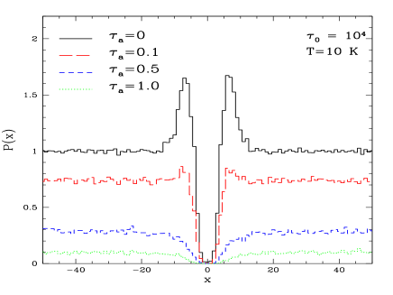
Figure 10: Emergent Ly$\alpha$ profiles for varying amounts of dust predicted for a slab with an isotropic source in the center emitting a flat continuum. The conditions of the medium are: $\tau_{0}=10^{4}$, $T=10$ K. In this static configuration, the two angular redistributions are equivalent; spectra have been obtained with the isotropic redistribution. The line profiles are shown for absorption dust optical depths of $\tau_{\rm a}=0.$ (no dust), 0.1, 0.5, 1. from top to bottom. Note the double-peak profile plus central absorption characteristic of a static medium for no dust. Already small amounts of dust are able to suppress the peaks, thereby leading to Voigt-like profiles. However, in such geometrical configurations, classical Voigt-profile fitting will underestimate the true HI column density. See text for more explanations.

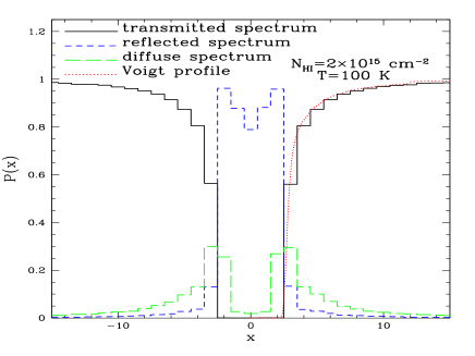
Figure 11: Predicted Ly$\alpha$ profiles of the direct transmitted (black solid line), the reflected (blue short-dashed), and the diffuse (green dotted) radiation from a static slab illuminated perpendicularly by a distant background source with a flat continuum. The properties of the intervening slab are: $N_{\rm H}=2.\,10^{15}$ cm^-2, $T=100$ K (i.e. $b=1.29$ km s^-1). The directly, i.e. perpendicularly, transmitted flux yields the expected Voigt profile (red dotted line). The diffuse (scattered) light shows again the double peak profile as the slab with a central source.

The “implicit” geometrical assumptions made above for the construction of an integrated spectrum are unlikely to be applicable to the typical damped Ly$\alpha$ systems (DLAs) observed in spectra of distant galaxies and quasars. These cases are better idealised by a small (in angular size) intervening cloud between the background source and the observer, which diffuses basically all photons out of the line of sight. In other words photons far from the line center will simply travel freely through the cloud, but when the photon frequency $x$ is close to the line center, the probability to cross the medium without interaction, $\exp(-\tau_{0}H(x,a))$, is considerably reduced. Since photons which interact with the medium have basically no chance to be re-emitted along the same line of sight (compare the observer solid angle with $4\pi$), they will be lost for the observer. Therefore the observed profile is simply that of a pure absorption line described by the Voigt absorption line profile, namely $I(x)=I_{0}\exp(-\tau_{0}\,H(x,a))$, reflecting the properties of the medium, i.e. the total column density and the temperature.

We simulated this configuration, and the resulting spectrum is presented on Fig 11, by the black curve. We checked again that a spheric cloud or a slab perpendicular to the line of sight, with the same optical depth and temperature, lead exactly to the same observed spectrum. For reasons of calculation time, we considered a relatively small column density, $N_{\rm H}=2\times 10^{15}cm^{-2}$. The temperature is set to $T=100K$. As expected, the simulation is perfectly fitted by a theoretical Voigt profile (red dotted curve). Also plotted on the same graph is the reflected spectrum (blue curve), composed of photons which escaped the medium by the side they entered.

Photons which are not “reflected”, i.e. backscattered to the source will diffuse in the medium and finally escape after a large number of scatterings forming the “diffuse spectrum”. For obvious reasons this spectrum, shown by the green curve, presents the same shape as the emergent spectrum from a slab with an isotropic source in the center, i.e. two symmetrical peaks. In dust-free cases with a flat incident continuum source, the transmitted spectrum will be the opposite of the reflected + diffuse spectrum, as all Ly$\alpha$ photons are conserved.

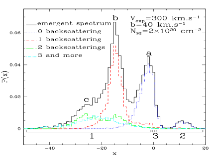
Figure 12: Left: Emergent Ly$\alpha$ profile from an expanding shell with central monochromatic source. The different shapes can be described with the number of back-scatterings photons undergo : bumps $1a$ and $2$ are built-up with photons which didn’t undergo any backscattering, the highest peak located at $x=-2V_{\rm exp}/b$ (feature $1b$) is composed of photons which undergo exactly one backscattering, and the red tail $1c$ is made of photons which undergo two or more backscatterings. See text for more details. Right: Scheme of an expanding shell showing the origin of photons of different groups. The observer is on the left side, at infinity.

In short, to form pure symmetric Ly$\alpha$ absorption line profiles from a flat continuum source requires specific geometrical configurations allowing the photons to diffuse out of the line of sight. An alternative way to achieve such profiles, e.g. in an integrated spectrum of an embedded source, is by invoking the presence of dust which destroys the double emission peaks otherwise present. However, in such a case the apparent column density derived from simple Voigt profile fitting underestimates the true value of $N_{\rm H}$ due to radiation transfer effects.

5 Ly$\alpha$ transfer in expanding dust-free and dusty shells revisited

There are numerous indications, both theoretically and observationally, for the presence of expanding shells and bubbles in starbursts. It is therefore important to simulate such geometrical configurations to examine both qualitatively and quantitatively the diversity of Ly$\alpha$ line profiles and to gain basic insight into the physical processes shaping them.

Our model of an expanding homogeneous shell is described by the following parameters: an inner and outer radius $R_{\rm min}$ and $R_{\rm max}$ respectively, a uniform radial expansion velocity $V_{\rm exp}$, the radial colunm density $N_{\rm H}$, and a constant temperature $T$ given by the Doppler $b$ parameter (Eq. 3). The interior of the shell is assumed to be empty, the isotropic Ly$\alpha$/continuum emitting source located at the center. In contrast to the geometrical configurations discussed earlier, emergent profiles from expanding shells are sensitive to the angular redistribution. Therefore the dipolar redistribution is taken into account to treat the Ly$\alpha$ radiation transfer consistently in this case, and all spectra shown in this section have been obtained using the dipolar redistribution in the code. The main parameters determining the Ly$\alpha$ photon escape and hence the line profile are $V_{\rm exp}$, $N_{\rm H}$, $b$, and the dust-to-gas ratio $M_{\rm d}/M_{\rm H}$, as shown below. The precise values of the shell radii and thickness, setting the geometrical size and curvature, are secondary.

Below we shall examine the following cases: The academic cases of a source with monochromatic emission and shells both without and with dust. These first two cases are essential to understand more realistic simulations allowing for arbitrary input spectra (including continuum and/or Ly$\alpha$ line emission), again dust-free or with dust, discussed subsequently.

5.1 Monochromatic emission and dust-free shells

5.1.1 Basic line profile formation mechanism

First we discuss the emergent Ly$\alpha$ spectrum from a dust-free expanding shell with the following parameters: $V_{\rm exp}=300$ km s^-1, $N_{\rm H}=2\times 10^{20}\,cm^{-2}$, $b=40$ km s^-1 (i.e. $\tau_{0}=3.8\times 10^{6}$), $R_{\rm min}=0.9R_{\rm max}$, and $R_{\rm max}=1.17\times 10^{19}$ cm. For monochromatic Ly$\alpha$ photons emitted at line center the resulting line profile is shown on the left panel of Fig 12 (solid black line). Qualitatively this line profile and others shown below exhibit the following characteristic features, marked on the figure and illustrated on the right panel:

• 1abc) an extended redshifted emission with one or two “bumps” (1a and 1b) and a red tail (1c) – all at $x<0$ (i.e. red side of Ly$\alpha$),

• 2) a smaller blue bump (at $x>0$), and

• 3) an narrow emission peak at the line center ($x=0$).

Although we considered the same physical conditions as Ahn et al. (2003, their Fig. 2), features 2) and 3) are not apparent in their simulations (cf. also Ahn 2004). However, these features are also found in the simulations of Hansen & Oh (2006) and the origin of all of them is well understood, as we shall now discuss. To do so it is instructive to group the emergent photons and to distinguish the emergent line profiles according to the number backscatterings they have undergone (see left panel on Fig. 12). A photon is said to “backscatter” when it travels across the empty interior before re-entering the shell at a different location (see right panel of Fig. 12). Note, that any such travel is counted as a backscattering, irrespective of its precise direction/length. In particular this does not necessarily imply a hemisphere change for the photon.

Features 1a and 2: photons with zero backscattering. In this simulation all photons are emitted at line center ($x=0$) at the center of the shell. Once a photon reaches the shell for the first time it is seen redshifted to $-x_{\rm CMF}(V_{\rm exp})=-7.5$ by the H atoms (in the comoving frame, CMF). A fraction of the photons will diffuse progressively through the shell towards the exterior and escape without backscattering (solid lines on the left panel of Fig. 12). Their spectrum (marked as 0 backscattering) gives rise to an asymmetric double peak with a small blue component centered at $x_{2}\sim 10$ (feature 2 above) from photons escaping the blue wing of Ly$\alpha$ in the (blueshifted) shell approaching the observer, and a somewhat redshifted stronger peak at $x_{1a}\sim-5$ (bump 1a above) corresponding to the photons escaping the red Ly$\alpha$ wing in the blueshifted shell. Qualitatively this part of the spectrum is equivalent to the spectrum of a slab with a constant receding macroscopic velocity with respect to the emitting source (see Neufeld 1990, Fig. 6).

Feature 3: direct escape. For sufficiently small column densities and/or large expansion velocities, a non-zero fraction of photons traverses directly the shell without interacting. This case appears with the probability $e^{-\tau_{\rm exp}(0)}$, where $\tau_{\rm exp}(x)=\tau(x-x(V_{\rm exp}))$ is the reduced Ly$\alpha$ optical depth seen by a photon with observers frequency $x$ due to Doppler shift of $V_{\rm exp}$. For the case discussed here $\tau_{\rm exp}(0)=\tau(-7.5)=6.09$, so that 0.25 % of the photons will escape without interacting. These photons give raise to feature 3 in the bin at $x_{3}=0$ labeled in Fig. 12. The importance of these direct photons increases of course with increasing $V_{\rm exp}$ and decreasing column density, as seen in Figs. 14 and 16. Before comparison with observed spectra this peaked flux contribution must obviously be convolved with the instrumental resolution.

Features 1b and 1c: photons undergoing one or more backscattering. Let us now examine the situation after one scattering in the expanding shell. After the first scattering the frequency distribution of the photons in the external frame is shown by the black solid line on Fig. 13. As the photons are initially seen by the atoms at the frequency $-x(V_{\rm exp})$, i.e. in the wings, they are basically re-emitted at the same frequency in the atoms frame. Depending on their emission direction this leads to a range of frequencies in the observer frame reaching from $x\sim-2x(V_{\rm exp})$ to 0, with more photons re-emitted in the absorption direction (around $x\sim-2x(V_{\rm exp})$) or in the opposite direction ($x\sim 0$) because of the dipolar angular redistribution (the frequency distribution for isotropic redistribution would be nearly a square profile over $x\sim[-2x(V_{\rm exp}),0]$). Which of these photons are now able to escape the medium after just one scattering is represented by the blue dotted histogram.

Overall, depending on their frequency being in one of the 3 spectral regions indicated in Fig. 13, the fate of the photons is as follows.

• Frequency range 1: Photons with a frequency $x_{\rm obs}\sim 0$ cannot escape the medium: they are emitted outward in the radial direction with a frequency too close to the line center (in the atoms frame). Their escape probability is negligible.

• Range 2: Around $x_{\rm obs}\sim-7.5$, although their frequency is far from line center, no photons escape the medium for geometrical reasons: their emission direction is perpendicular to the radial direction increasing thus strongly the geometrical path and the optical depth.

• Range 3: Most of the photons escape with a frequency $x_{\rm obs}\la-9$ since their frequency is very far from line center, and their emission direction is convenient: they cross the inner part of the shell (backscattering), and when they arrive on the other side, the combination of their frequency and direction with the local macroscopic motion favours their escape. The frequency distribution function after one scattering shows that the number of photons re-emitted with a frequency $x<-2x(V_{\rm exp})$ decreases very rapidly. Therefore the photons escaping after just one scattering already show a peak close to the frequency corresponding to twice the expansion velocity. So a peak of escaping photons centered at the frequency $x=-2x(V_{\rm exp})$ appears.

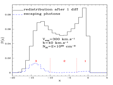
Figure 13: Frequency distribution of the photons in the expanding shell after the first scattering. The black solid curve contains all photons, the blue dotted one represents the histogram of photons which escaped after only one scattering. bf They form a bump around $x\sim-2x(V_{\rm exp})$ which explains the appearance of feature 1b. See the text for more details.

Photons undergoing further scatterings will be absorbed again, and the escape of those re-emitted around $-2x(V_{\rm exp})$ will be favoured again for same reasons. This explains why the most prominent feature (1b) in the red part is located at $x_{1b}\sim-2x(V_{\rm exp})$, measuring therefore twice the shell velocity. Photons undergoing progressively more scatterings will show a broadening frequency distribution compared to that after one scattering. The broadening of its red wing is responsible for the last feature (1c) made of photons escaping after 2 or more backscatterings.

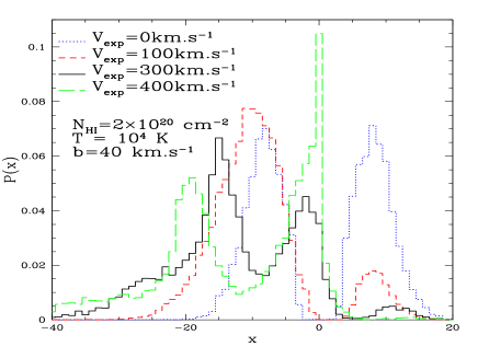
Figure 14: Dependence of the predicted Ly$\alpha$ profiles from an expanding shell with a central monochromatic source on the expansion velocity.

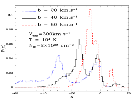
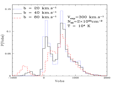
Figure 15: Dependence of the predicted Ly$\alpha$ profiles from an expanding shell with a central monochromatic source on the Doppler parameter $b$. As the characteristic unit of Ly$\alpha$ radiative transfer problem, $x$, depends on the Doppler parameter $b$(cf. Eq. 4), a variation of $b$ will lead to a change of $x$ too. To compare cases with different $b$, we show the usual plot in $x$ units but also a plot in velocity. Left: Plot in Dopper units $x$, Right: Plot in velocity along the line of sight $v_{\rm obs}$.

5.1.2 Dependence on shell parameters

Another way to understand the different features of the emergent Ly$\alpha$ line profile of an expanding shell is by varying the parameters. Let us examine how the spectrum depends on the expansion velocity $V_{\rm exp}$, on the thermal and turbulent velocities intervening in the Doppler parameter $b$, and on the colunm density $N_{\rm H}$.

For increasing expansion velocities, and starting from the static case with a symmetric double peak profile (cf. above and Eq. B18 of Dijkstra & Haiman 2005a for a static sphere), the imbalance between the red part and the blue part grows (see Fig. 14): progressively more photons escape from the red part of the line because atoms see them already redshifted (red dashed curve) at the first interaction. The probability to be re-emitted in the line core is then smaller than the one to “remain” in the wing. Hence the growing asymmetry between red and blue. Note also the appearance of excess flux at line center for the curve with the highest $V_{\rm exp}$ in Fig. 14. The appearance and strength of this feature ($x_{3}=0$, feature 3) is consistent with the increasing direct escape probability.

For a given $b$, the red part is a single peak, for small enough values of $V_{\rm exp}$ (e.g. $V_{\rm exp}<200$ km s^-1 for $b=40$ km s^-1). In fact, the two contributions of photons undergoing zero and one backscattering are then too close to be distinguished, and the two corresponding red peaks (features 1a and 1b) are mixed. The same trend is found for large values of $b$, as shown in the left panel of Fig. 15. More precisely, predicted Ly$\alpha$ profiles from an expanding shell present only one red peak for sufficiently small $V_{\rm exp}/b$. With increasing $V_{\rm exp}$ or decreasing $b$, the blue part (feature 2) becomes very faint, and almost all photons escape in the red part, presenting two well separated peaks. In all cases, and quite independently of $b$ (cf. Fig. 15, left), the second and most prominent peak (feature 1b) traces twice the expansion velocity as already discussed above. It is essentially composed of photons which undergo one backscattering, while the first peak (feature 1a) is made of photons undergoing no backscattering. Note, however, that in contrast to the appearance in this plot, the position of main peak is independent of $b$ in observed spectra, as illustrated in the right panel of Fig. 15. This is simply due to the definition of $x$, which depends on $b$.

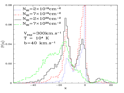
Figure 16: Dependence of the predicted Ly$\alpha$ profiles from an expanding shell with a central monochromatic source on the column density.

Varying the column density (leaving the other parameters unchanged) has the following effects (see Fig 16). First, the flux excess at $x_{3}=0$, i.e. the fraction of photons which can escape the shell without interacting, decreases exponentially with increasing $N_{H}$. Second, the relative importance of the two red peaks (1a, 1b) changes: with increasing column density the first peak (feature 1a) decreases with respect to the second one (1b), whereas the red wing (1c) is enhanced, since the importance of backscattering increases. For sufficiently large $N_{H}$ the first peak (1a) disappears completely, whereas the red tail (1c) becomes as important as the mean peak (1b).

In short, the imbalance between blue and red emission increases with increasing $V_{\rm exp}/b$. The separation between the multiple peaks formed on the red side of the Ly$\alpha$ profile becomes progressively less clear (i.e. the peaks merge together) for lower expansion velocities, and/or higher temperature or turbulent velocities. For sufficiently large H i column densities ($N_{\rm H}$ $\ga 10^{20}$ cm^-2) the main red emission peak measures quite well $2V_{\rm exp}$.

5.2 Monochromatic emission and dusty shells

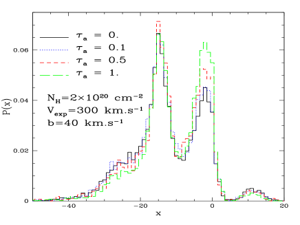
Figure 17: Predicted emergent Ly$\alpha$ profiles from an expanding shell with a monochromatic central source with a column density $N_{\rm H}=2\times 10^{20}$ cm^-2, an expansion velocity $V_{exp}=300$ km s^-1  a Doppler parameter $b=40$ km s^-1, and different dust absorption optical depths $\tau_{a}=$0., 0.1, 0.5, and 1.0. The area under each curve is normalised to unity, i.e. corrected for photon destruction by dust, to highlight the relatively minor line profile changes. The blue bump (2) and the red tail (1c) are more destroyed by dust than other features. Overall the profile is globally preserved, but somewhat “sharpened”.

In Fig. 17 we present the influence of dust on the emergent spectrum from the expanding shell studied above (Fig 12). When $\tau_{a}$ increases, the relative height of the two red peaks (features 1a and 1b) is reversed: in dust-free media the prominent peak is 1b, but when dust is present 1a becomes as high as 1b. In the most dusty cases, corresponding to a destruction of $\sim$ 93% of Ly$\alpha$ photons, one notes a loss of photons from the the blue bump (feature 2 on Fig. 12) and from the red tail (feature 1c on Fig 12). This is easily understood as these features are composed of photons undergoing a very large number of scattering, which increases their chance to be absorbed by dust. Qualitatively our results show the same behaviour as the outflowing shell with holes or clumps modeled by Hansen & Oh (2006): strongly redshifted photons are suppressed by dust, whereas the spectral peaks are still visible. The result is a somewhat “sharpened” line profile. Although this overall “sharpening” trend is also found in the earlier simulations of Ahn (2004) our results differ quite strongly from theirs, as already mentioned above.

We now quantify the Ly$\alpha$ photon destruction by dust and its dependence on the shell and dust parameters. For illustration we have chosen similar conditions as those discussed by Ahn (2004), namely a shell with an inner and outer radius $R_{\rm min}=0.9R_{\rm max}$, an expansion velocity $V_{\rm exp}=200$ km s^-1, a H i column density between $N_{\rm H}=10^{19}$ and $10^{21}$ cm^-2, a Doppler parameter of $b=$ 20, 40, and 80 km s^-1, and a monochromatic central point source. In contrast to Ahn (2004) we assume that there is no dust inside the bubble, i.e. at $R<R_{\rm min}$, as most of the dust is probably destroyed there. Furthermore, the presence of dust inside the shell is not compatible with inferences from the empirical Calzetti attenuation law (see e.g. Gordon, Calzetti & Witt 2003). The predicted Ly$\alpha$ escape fraction as a function of the dust absorption optical depth $\tau_{a}$ measuring, for a given $N_{\rm H}$ column density, different dust-to-gas amounts, is shown in Fig. 18.

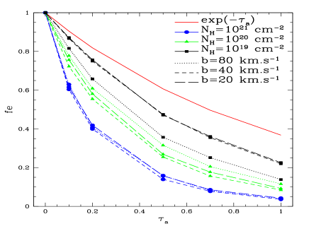
Figure 18: Escape fraction of Ly$\alpha$ photons from an expanding shell with $V_{\rm exp}$=200 km s^-1for different column densities ($N_{\rm H}=10^{19}$, 10²⁰, $10^{21}$ cm^-2) and for different Doppler parameters ($b=$20, 40 and 80 km s^-1).

As expected, the main dependence of the escape fraction $f_{e}$ is on $N_{\rm H}$ and $\tau_{a}$. Due to the multiple resonant scattering of Ly$\alpha$ photons on hydrogen and the concomitant increase of the photon path length, $f_{e}$ is considerably smaller than the simple dust absorption probability $\exp(-\tau_{a})$, and the escape fraction decreases strongly with increasing $N_{\rm H}$.

In an expanding shell the Ly$\alpha$ photon destruction by dust depends also to some extent on the gas temperature (or on the Doppler parameter $b$), although in a somewhat “subtle” way as can be seen from Fig. 18. Indeed, for large column densities (here $N_{\rm H}$ $>10^{20}$) $f_{e}$ is found to depend little on $b$, for intermediate values of $N_{\rm H}$ $\sim 10^{20}$ the escape fraction varies in a non-monotonous way with $b$, and for lower $N_{\rm H}$ values $f_{e}$ decreases with increasing $b$. This latter behaviour is opposite to the one in a static medium, where the escape fraction increases with $b$ (cf. Fig. 4 or Eq. 23 with $a\propto b^{-1}$ and $\tau_{0}\propto b^{-1}$). The reason for this inverted dependence is basically due to the fact that in an expanding shell the quantity $V_{\rm exp}/b$ determines the frequency at which the initially emitted photons are seen by the atoms in the receding shell. For increasing $b$, $V_{\rm exp}/b$ decreases, so that photons reaching the shell are seen with a frequency closer to line center. Hence they will diffuse more and will have a higher probability to be absorbed by dust. On the contrary, when $b$ decreases, photons are seen in the wings, their chance to interact with dust decreases and so does $f_{e}$. When they are sufficiently far from line center ($V_{\rm exp}/b\gg x_{c}$, where $x_{c}$ is some critical frequency), the shell becomes transparent in Ly$\alpha$ and the escape fraction approaches the minimum value given by the dust absorption probability $\exp^{-\tau_{a}}$ (red upper curve on Fig. 18).

5.3 Dust-free and dusty shells with arbitrary source spectra

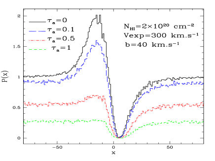
Figure 19: Predicted Ly$\alpha$ profiles for an expanding shell for a central source emitting a flat continuum and with different amounts of dust. The adopted conditions are the following: $N_{H}=2.\,10^{20}$ cm^-2, $T=10000$ K, $b=40$ km s^-1, and $V_{\rm exp}=300$ km s^-1. The line profiles are shown for dust amounts corresponding to ($M_{d}/M_{H}$, $\tau_{a}$) = (0., 0.), ($8.\,10^{-4}$, 0.1), ($4.\,10^{-3}$, 0.5), ($8.\,10^{-3}$, 1.).

Now we present the emergent spectrum from an expanding shell when the input spectrum is a flat continuum and with different amounts of dust. In Fig. 19, the black solid line represents the emergent spectrum from a dust-free shell. It is a P-Cygni profile, quite similar to the expanding halo with a central point source in Fig. 8. Again, Ly$\alpha$ radiation transfer leads to the appearance of an emission peak and an absorption feature in the emergent profile which did not exist in the input spectrum. The first remark is that this spectrum is less complex than in the monochromatic case: there is only one red peak, and no blue bump, due to radiation transfer of photons at all frequencies. The emission peak is located at $x\sim-2x(V_{\rm exp})$, as the highest peak of the monochromatic spectrum, and the absorption is around $x\sim x(V_{\rm exp})$, as this frequency corresponds to the line center frequency in the shell frame. The effect of dust is similar to Fig. 8 for spherical halos: it suppresses the emission peak and broadens the absorption, leading to an asymmetric absorption profile. The fraction of escaping photons far from the line center is equal to $\exp(-\tau_{a})$, as expected (see discussion section 3.2.2).

Figure 20: Predicted Ly$\alpha$ profiles from an expanding shell with a central source emitting a flat continuum plus a monochromatic line (at Ly$\alpha$ line center) with different equivalent widths. The physical conditions in the shell are: a H i column density $N_{\rm H\leavevmode\nobreak\ {\sc i}}=2\times 10^{20}$ cm^-2, a temperature $T=10^{4}$ K, a Doppler parameter $b=40$ km s^-1, no dust, and a radial velocity of $V_{\rm exp}=300$ km s^-1. The Ly$\alpha$ line equivalent width, given in units of the Doppler width $\Delta\nu_{D}$, increases from $0$ to $\infty$ from the top-left to the bottom-right panel.

To illustrate the variety of emergent line profiles from a dust-free expanding shell when varying the intrinsic line strength, we show in Fig.  20 a family of emergent spectra with intermediate cases between intrinsic pure continuum (cf. Fig.  19) and intrinsic monochromatic emission (cf. Fig.   12). For a sufficiently large Ly$\alpha$ equivalent width $W({\rm Ly}\alpha)$, the second red peak (feature 1a), the small excess at $x=0$ (feature 3) and the blue bump (referred to as feature 2) become clearly visible.

6 Ly$\alpha$ line profile morphologies – models and qualitative comparison with observations

For a better overview over the different simulations presented here and the resulting variety of Ly$\alpha$ line profiles, and for a first qualitative comparison with observations we present a summary in Table 1.

Table 1: Schematic overview over the different simulations, the resulting line profile morphologies, and observed objects showing qualitatively similar profiles. Column 1 describes the adopted geometry, col. 2 describes the source position and spectrum, col. 3 the predicted line profile morphology, col. 4 the corresponding figure in the paper, and col. 5 possible objects showing qualitatively similar profiles.

Case	Geometry	Source	Line profile	Figure	Observations
1	static medium	embedded source,	2 symmetrical peaks	Fig. 1	LAB2?1
		monochromatic	at $x_{p}=\pm(a\tau_{0})^{1/3}$
2	static medium	embedded source,	2 symmetrical peaks if no dust	Fig. 10
		continuum	DLA profile not related to $\tau_{0}$ if dust		IZw18,SBS0335-052? 2
3	static medium	external source,	DLA profile	Fig. 11	DLA3
		continuum	+ faint diffuse component
4	expanding/infalling halo	central source,	asymmetric emission peak	Figs. 5, 9
		monochromatic
5	expanding/infalling halo	central source,	P-Cygni without dust	Figs. 8, 9
		continuum	asymmetric absorption profile if dust
6	expanding shell	central source,	1-2 red peaks (main peak at $\sim 2V_{\rm max}$),	Figs. 12–16, 20	LBGs4, low-$z$ starbursts2
		monochromatic	one blue peak
7	expanding shell	central source,	P-Cygni without dust	Figs. 19, 20
		continuum	asymmetric absorption profile if dust		IZw18,SBS0335-052? 2
References: 1 Wilman et al. (2005), 2 Mas-Hesse et al. (2003), 3 Adelberger et al. (2005), 4 see e.g. Shapley et al. (2003) and Noll et al. (2004)

Schematically we may classify the emergent Ly$\alpha$ profiles and considered geometries in the three following main groups, 1) static media and symmetric profiles, 2) expanding/infalling halos, and 3) expanding shells, which we shall discuss now.

6.1 Static media, symmetric profiles

For simple static geometries with an embedded source emitting a symmetric spectrum around $x=0$ (i.e. monochromatic line radiation, a symmetric line centered on the Ly$\alpha$ in the restframe of the medium, or a flat continuum) the emergent Ly$\alpha$ line profile remains symmetric with two peaks, whose position is given by $x_{p}\approx\pm(0.9-1)\times(a\tau_{0})^{1/3}$ and little or no flux at line center (case 1 in Table 1; cf. Neufeld 1990, Hansen & Oh 2006). The detailed line shape (FWHM of each part, the possible presence of “bumps” etc.) depends on the properties of the scattering medium in ways quantified in detail by Neufeld (1990) and examined also by Richling (2003) for clumpy media. Breaking the symmetry of the source spectrum or introducing velocity shifts between the source and the scattering medium lead to asymmetric profiles, as well known (cf. Neufeld 1990).

Emission peaks superposed to a continuum – e.g. from a source with a pure continuum or continuum plus line emission – are easily “destroyed” in presence of dust (case 2). In this case the resulting profile is close to a Voigt profile. However, due to radiation transfer effects and the assumed geometry and “aperture”, an integrated line profile fit in this manner will underestimate the true value of the column density.

Purely or close to symmetric Ly$\alpha$ line profiles are quite rarely observed. E.g. the spectra of the Ly$\alpha$ blob LAB2 at $z\sim 3.09$ of Steidel et al. (2000) observed by Wilman et al. (2005), Ly$\alpha$ emitters around a radio galaxy (Venemans et al. 2005), or two LBG in the FORS Deep Field (Tapken 2005) come close to this, and may hence be related to static (or close to) media. For LAB2, however, other explanations have been put forward by Wilman et al. (2005) and Dijkstra et al. (2005b) including outflows + “absorbing screens” and intergalactic medium (IGM) inflow.

Some nearby starbursts such as I Zw 18 and SBS 0335-052 show bf “Voigt-like” profiles (cf. Kunth et al. 1994, Thuan & Izotov 1997, Mas-Hesse et al. 2003). If related to a continuous source embedded in an H i cloud (case 2), such profiles can be reproduced with sufficient dust. In this case the H i column density derived from simple Voigt profile fitting would underestimate the true value. Other configurations can, however, also lead to the same profiles. To clarify such ambiguities, a detailed analysis taking all known constraints into account will be necessary.

A static medium illuminated by a distant background continuum source (case 3) produces well known Voigt absorption line profiles, e.g. seen as damped Ly$\alpha$ absorbers (DLA). In such a geometry Ly$\alpha$ radiation transfer effects need not be considered. A case of “Ly$\alpha$ fluorescence” of QSO radiation on a nearby absorbing system has been observed recently by Adelberger et al. (2005): they detected a double-peaked emission superimposed on a DLA profile. This can be related to our diffuse spectrum illustrated in Fig 11.

6.2 Expanding/infalling halos

As already discussed by Zheng & Miralda-Escudé (2002) and Dijkstra et al. (2005a) for monochromatic sources emitting at line center, such geometries give rise to asymmetric profiles with a redshifted (blueshifted) main peak for expanding (infalling) matter, and eventually secondary features (case 4). The position of the main peak shows the same dependence as for a Hubble outflow (Loeb & Rybicky 1999): it moves away from line center with increasing $N_{\rm H}$ and decreasing velocity $V_{\rm max}$. In the case of uniform emissivity, the positions of the secondary peak and the point of minimal flux indicate the external velocity (see Fig. 8 in Dijkstra et al. 2005a).

For sources emitting a pure continuum, the Ly$\alpha$ radiation transfer leads to normal (inverted) P-Cygni profiles for expanding (infalling) halos. Again, as for static media, the presence of dust is able to destroy the emission peak leading then to absorption line profiles with more or less pronounced asymmetries (case 5).

Dijkstra et al. (2005b) have argued for possible infalling Ly$\alpha$ halos in the case of the Ly$\alpha$ blob LAB2 of Steidel et al. (2000), and of a $z=5.78$ galaxy discovered by Bunker et al. (2003). Numerous LBGs and LAEs show asymmetric redshifted Ly$\alpha$ profiles, which could in principle be related to expanding halos. To distinguish this geometry from expanding shells or other geometries additional observational constraints are needed. For $z\sim 3$ LBGs, for example, expanding shells provide a good description, as we’ll discuss now.

6.3 Expanding shells

Emergent Ly$\alpha$ profiles from an expanding shell can be rather complex: from P-Cygni profiles or asymmetric absorption profiles for an intrinsic continuum spectrum (case 7) to emission line profiles made of one (or two) red peaks and possibly a fainter blue bump for an intrinsically monochromatic (line) spectrum (case 6). In all cases the profiles show an asymmetric red wing related to Ly$\alpha$ scattering in the outflowing medium. When Ly$\alpha$ is in emission, the velocity shift of the main peak of the red part of the profile corresponds to velocities between $V_{\rm exp}$ and $\sim 2V_{\rm exp}$, where $V_{\rm exp}$ is the expansion velocity of the shell. For column densities $N_{\rm H}$ $\ga 10^{20}$ cm^-2 the main red emission peak measures quite accurately twice the shell velocity.

Interestingly, spectroscopic observations of Lyman break galaxies (LBG) at $z\sim 3$ agree very well with the expectations for an expanding shell geometry. Indeed the composite spectra of the large LBG samples of Shapley et al. (2003) show not only clear signatures of outflows, as testified by a shift between Ly$\alpha$ emission and interstellar absorption lines (with a mean value of $\Delta\nu_{\rm em-abs}\sim$ 650 km s^-1). The low-ionisation interstellar absorption lines are found blueshifted by $\Delta\nu=-150\pm 60$ km s^-1 with respect to the stellar, systemic redshift, whereas the Ly$\alpha$ emission is found redshifted by $\Delta\nu=+360$ km s^-1 (Shapley et al. 2003), i.e. quite precisely at twice the velocity measured by the interstellar (IS) absorption lines. As the latter are formed by simple absorption processes, i.e. by intervening gas on the line of sight between the continuous source (the starburst) and the observer, whereas Ly$\alpha$ is prone to complex radiation transfer effects, the above empirical finding together with our modeling insight indicates very clearly that on average the distribution and kinematics of the ISM in these LBGs is well described by an expanding shell. This is quite naturally the most simple geometry to simultaneously explain IS absorption lines blueshifted by an outflow velocity $V_{\rm exp}$ and an asymmetric Ly$\alpha$ line redshifted by twice this velocity!

As these two spectral features are formed on opposite hemispheres, IS absorption lines on the side approaching the observer and Ly$\alpha$ from photons scattered back from the receding shell (cf. Pettini et al. 2001), this implies that overall (or “on average” over an entire LBG sample) the ISM shell structure must be fairly spherically symmetric rather than e.g. strongly bipolar. Such a structure may indeed be expected in case of strong starbursts triggering efficient large scale outflows (see e.g. simulations of Mori et al. 2002).

For a shell geometry the finding of a velocity shift of $\sim 3V_{\rm exp}$ between Ly$\alpha$ and the IS absorption lines also requires a large enough H i column density (cf. above). This is fully compatible with the typical/average value of $N_{\rm H}$ of the $z\sim 3$ LBG sample of (Shapley et al. 2003) expected from the standard correlation between $N_{\rm H}$ and the extinction $E_{B-V}$.

Finally we note that the relatively smooth, singly peaked Ly$\alpha$ line profiles observed by Shapley et al. (2003) and others are not in contradiction with our predictions. As already explained above, there are several ways to avoid the multiple peaks predicted for certain conditions on the red side of Ly$\alpha$ (e.g. Figs. 14 to 16): among them are low expansion velocities, high column densities, or large Doppler parameters and combinations thereof. Actually, for the relatively low outflow velocity of $V_{\rm exp}\sim 150\pm 60$ km s^-1 deduced from the Shapley et al. (2003) sample, and taking into account their relatively low spectral resolution, no distinguishable multiple red peaks are expected. At least for this sample, the problem posed by Ahn (2004) to avoid multiply peaked Ly$\alpha$ profiles is ill posed. The possible but generally minor blue peak, which is predicted but not observed, does not pose a problem; in these high redshift objects it may be too faint to be detected or actually suppressed by the intervening interstellar H i clouds in the galaxy.

Local starbursts (see e.g. Kunth et al. 1994, 1998, González Delgado et al. 1998, Mass-Hesse et al. 2003) present P-Cygni profiles with a faint secondary peak on the blue side superimposed to the absorption feature (e.g. IRAS 0833+6517), or more or less symmetric absorption profiles (e.g. IZw 18, SBS 0335-052). Mass-Hesse et al. (2003) interpret the variety of observed Ly$\alpha$ profiles as phases in the time evolution of an expanding supershell. Few galaxies of those showing P-Cygni profiles have measurements of the relative velocities between the interstellar absorption lines, Ly$\alpha$, and the ionised gas (traced e.g. by H$\alpha$). Although, e.g. in Haro 2 the shift between Ly$\alpha$ and the interstellar lines is $\sim 2V_{\rm exp}$, their spectra are a priori not in contradiction with our simulations, as velocity shifts $<3V_{\rm exp}$ are obtained for neutral column densities in the shell smaller than $10^{20}$ cm^-2, in agreement with the value derived by Lequeux et al. (1995). Furthermore, the secondary peak on the blue side of the P-cygni profiles is easily reproduced by Ly$\alpha$ radiation transfer through a superbubble. This is maybe the strongest indication for such a geometry. Detailed modeling of these nearby galaxies, taking all available observational constraints and spatial information into account, is necessary to shed more light onto these questions.

6.4 General comments

As the above shows, the expected Ly$\alpha$ profiles show already quite a complexity depending on the values of the main parameters considered (geometry, H i distribution and column density, velocity field, Doppler parameter, dust to gas ratio, and input spectrum) and important degeneracies are found. Overall it is quite clear from this study and earlier ones that radiation transfer effects are important to shape the emergent Ly$\alpha$ profile. The interpretation of observed P-Cygni profiles or asymmetric emission lines, for example, requires full radiation transfer calculations rather than superpositions of gaussian emission and Voigt-like absorption profiles as undertaken in various studies (e.g.  Mas-Hesse et al. 2003, Wilman et al. 2005). Such a detailed comparison with observations will be presented elsewhere.

Obviously the geometries adopted in this paper are strongly idealised when compared to real galaxies. Asymmetries, non-unity filling or covering factors, arbitrary geometries, and effects of different viewing and opening angles have to be considered for more realistic simulations. Although our code can treat arbitrary density distributions, we have so far only investigated homogeneous media. For complementary approaches treating clumpy media see e.g. Neufeld (1991), and Hansen & Oh (2006). Furthermore, in addition to the simple limiting cases of input spectra (monochromatic line plus continuum), other cases such as intrinsic Gaussian emission lines must be accounted for. All of these effects can easily be modeled with our generalised 3D radiation transfer code, and will be discussed in future applications.

Beyond the Ly$\alpha$ radiation transfer modeled here for simplified “galaxian” geometries it should be recalled that Ly$\alpha$ line profiles predicted in this manner are still a priori prone to alterations due to the transmission through the intervening IGM., As well known (e.g. Madau 1995) this effect can significantly alter observed Ly$\alpha$ line profiles — especially on the blue side — for objects of sufficiently high redshift (typically $z\ga\ 3$). Effects of the IGM have e.g. been discussed by Haiman (2004), Santos (2004), and Dijkstra et al. (2005b), and are not treated here. For most purposes the IGM effects can be computed without the need for true Ly$\alpha$ radiation transfer calculations.

7 Summary and conclusion

We have developed a new general 3D Ly$\alpha$ radiation transfer code allowing for arbitrary hydrogen density, ionisation & temperature structures, dust distributions, and velocity fields using a Monte Carlo technique (Sect. 2). Currently the code works on a cartesian grid and it can handle Ly$\alpha$ transfer problems in objects with arbitrary hydrogen column densities. The main radiation–matter interaction processes included in the code are Ly$\alpha$ scattering, dust scattering, and dust absorption. UV/Ly$\alpha$ photon sources with an arbitrary spatial distribution and arbitrary spectra can be treated. The main direct observables predicted by our simulations are “global” (i.e. integrated over all viewing angles) Ly$\alpha$ line profiles, spectra for different viewing directions and opening angles, and surface brightness maps at different wavelengths (or integrated over Ly$\alpha$).

The code has been tested successfully and compared against analytical results and results from other simulations (e.g. Neufeld 1990, Ahn et al. 2001, Zheng & Miralda-Escudé 2002, Richling et al. 2003, Dijkstra & Haiman 2005a) for various geometrical configurations including plane parallel slabs, disks, and expanding or infalling halos, and for computations with and without dust. Overall an excellent agreement is found, except in cases where assumptions made in the analytical calculation break down (see Sect. 3).

With the aim of understanding and interpreting ultimately the variety of Ly$\alpha$ profiles observed in nearby and distant starbursts, we have examined the Ly$\alpha$ line profiles predicted for several simple geometrical configurations and their dependence on the main parameters such as the H i column density, temperature, velocity, and dust content. We have considered slabs with internal sources, disks, expanding and infalling halos (Sect. 3), externally illuminated slabs (Sect. 4), and expanding shells (Sect. 5). For the source spectrum we have considered the limiting cases of pure monochromatic line emission, a pure continuum, or intermediate cases with different line strengths. The two latter cases have rarely been discussed in the literature so far.

Schematically, the following morphologies are found (cf. Table 1): profiles reaching from doubly peaked symmetric emission to symmetric ”Voigt-like” (absorption) profiles in static configurations with increasing dust content, and asymmetric red- (blue-) shifted emission lines with a blue (red) counterpart ranging from absorption to emission (with increasing line/continuum strength) in expanding (infalling) media. In principle, symmetric or nearly symmetric profiles are only obtained for static geometries or for small systematic velocities. In practice, however, this may be altered by Ly$\alpha$ scattering/absorption in the intervening IGM, especially at high redshift.

Some specific results are worthwhile summarising here:

• Pure Ly$\alpha$ absorption line profiles may be observed in “integrated”/global spectra of objects with static geometries. In this case the naturally arising double Ly$\alpha$ emission peaks have been suppressed by dust absorption. Standard Voigt profile fitting of such profiles will significantly underestimate the true hydrogen column density (see Sect. 4).

• It should be noted that normal (inverted) P-Cygni like Ly$\alpha$ profiles can be obtained in expanding (infalling) media from objects without any intrinsic Ly$\alpha$ emission, as a natural consequence of radiation transfer effects redistributing UV (continuum) photons from the Ly$\alpha$ line center to the red (blue) wing (e.g. Figs. 9, 20). Adding dust in such cases will progressively transform the P-Cygni profile into a broad asymmetric absorption profile.

• Our 3D simulations of expanding shells lead us to revise the earlier results of Ahn and collaborators (Ahn et al. 2003, Ahn 2004) and to clarify the radiation transfer processes explaining the detailed shape of Ly$\alpha$ profiles predicted from expanding shells. In particular we found that, for sufficiently large column densities ($N_{\rm H}$ $\ga 10^{20}$ cm^-2), the position of the main Ly$\alpha$ emission peak is quite generally redshifted by approximately twice the expansion velocity (Sect. 5). This is in excellent agreement with the observations of $z\sim 3$ LBGs from Shapley et al. (2003), which show that Ly$\alpha$ is redshifted by $\sim 2V_{\rm exp}$, where $V_{\rm exp}$ is the expansion velocity measured from the interstellar absorption lines blueshifted with respect to the stellar (i.e. galaxian) redshift. This finding indicates also that large scale, fairly symmetric shell structures must be a good description for the outflows in LBGs.

As already clear from earlier investigations, radiation transfer effects even in the simple configurations just mentioned give rise to a complex morphology of Ly$\alpha$ line profiles and some degeneraciesare found e.g. between the main parameters such as the hydrogen column density $N_{\rm H}$, the Doppler parameter $b$, and also the intrinsic emission line width. However, codes as the one developed and presented here allow one to undertake detailed Ly$\alpha$ line profile fitting to determine the physical properties of the emitting gas and of the surrounding H i and dust and to quantify possible degeneracies. With such tools it is now possible to fully exploit the information encoded in Ly$\alpha$ profiles without recurring to physically unmotivated superpositions of emission and Voigt absorption line profiles, which – except in specific geometric configurations – generally do not properly account for radiation transfer effects. Such detailed studies of nearby and distant starforming galaxies will be presented in subsequent publications. Various other applications, combining also our MCLya code with the 3D radiation transfer and photoionisation code CRASH (Maselli et al. 2003) are foreseen.

- (1) Adelberger, K. L., Steidel, C. C., Kollmeier, J. A., Reddy, N. A. 2006, ApJ, 637, 74A
- (2) Ahn, S.H., Lee, H.W., Lee, H.M., 2001, ApJ, 554, 604
- (3) Ahn, S.H., Lee, H.W., Lee, H.M., 2002, ApJ, 567, 922
- (4) Ahn, S.H., Lee, H.W., Lee, H.M., 2003, MNRAS, 340, 863
- (5) Ahn, S.H., 2004, ApJ, 601, L25
- (6) Bunker, A.J., et al., 2003, MNRAS, 342, L47
- (7) Calzetti, D., et al., 2000, ApJ, 533, 682
- (8) Cantalupo, S., et al., 2005, ApJ, 628, 61
- (9) Charlot, S., Fall, S. M. 1993, ApJ, 415, 580
- (10) Dijkstra, M., et al., 2005a, in press [astroph/0510407]
- (11) Dijkstra, M., et al., 2005b, in press [astroph/0510409]
- (12) Djorgovski, S., Thompson, D. J., Smith, J. D., Trauger, J. 1992, A&AS, 181, 7906
- (13) Field, G.B., 1959, ApJ, 129, 551
- (14) González Delgado, R.M., Leitherer, C., Heckman, T.M., Lowenthal J.D., Ferguson, H.C., Robert, C., 1998, ApJ, 495, 698
- (15) Gordon, K. D., Calzetti, D., Witt, A. N. 1997, ApJ, 487, 625
- (16) Gray, D. F., Observations and Analysis of Stellar Photospheres -Ed2, SCIENCE V.257, NO.5078, SEP25, P.1978, 1992.
- (17) Haiman, Z., 2002, ApJ, 576, L1
- (18) Hansen, M., Oh, S.P., 2006, MNRAS, 367, 979
- (19) Harrington, J.P., 1973, MNRAS, 162,43
- (20) Hartmann, L. W., Huchra, J. P., Geller, M. J. et al. 1988, ApJ, 326, 101
- (21) Hu, E., et al., 1998, ApJ, 502, L99
- (22) Hu, E., et al., 2004, AJ, 127, 3137
- (23) Hummer, D.G., 1962, MNRAS, 125, 21
- (24) Kobayashi, M. A. R., Kamara, H. 2004, ApJ, 600, 564
- (25) Kudritzki et al. 2000, ApJ, 536, 19
- (26) Kunth, D., Lequeux, J., Sargent, W.L., Viallafond, F., 1994, A&A, 282, 709
- (27) Kunth et al. 1998, A&A, 334. 11
- (28) Lequeux, J., Kunth, D., Mas-Hesse, J.M., Sargent, W.L., 1995, A&A, 301, 18
- (29) Loeb, A., Rybicki, G.B., 1999, ApJ, 524, 527
- (30) Madau, P. 1995, ApJ, 441, 18
- (31) Maselli, A., et al., 2003, MNRAS, 345, 379
- (32) Mas-Hesse et al. 2003, ApJ, 598, 858
- (33) Meier, D. L., Terlevich, R. 1981, ApJ, 246, 109
- (34) Möller, P., Fynbo, J. P. U., Fall, S. M., A&A, 422, 33
- (35) Mori, M., Ferrara, A., Madau, P. 2002, ApJ, 571, 40
- (36) Neufeld, D.A., 1990, ApJ, 350, 216
- (37) Neufeld, D.A., 1991, ApJ, 370, 85
- (38) Noll, S., et al., 2004, A&A, 418, 885
- (39) Ouchi, M., et al., 2003, ApJ, 582, 60
- (40) Partridge, R. B., Peebles, J. E. 1967, ApJ, 147, 868
- (41) Pettini, M., Steidel, C. C., Adelberger, K. L. et al. 2000, ApJ, 528, 96
- (42) Pettini, M., Rix, S. A., Steidel, C. C. et al. 2002, ApJ, 569, 742
- (43) Rhoads et al. 2000, ApJ, 545, 85
- (44) Richling, S., et al. 2001, A&A, 380, 776
- (45) Richling, S., 2003, MNRAS, 344, 553
- (46) Rybicki, G.B., Loeb, A., 1999, ApJ, 524, 527
- (47) Seaton, M.J., 1979,MNRAS, 187, 73
- (48) Santos, M.R., 2004, MNRAS, 349, 1137
- (49) Shapley, A., Steidel, C. C., Pettini, M., Adelberger, K. L. 2003, ApJ, 588, 65
- (50) Spaans, M., 1996, A&A, 307, 271
- (51) Steidel, C., et al., 2000, ApJ, 532, 170
- (52) Taniguchi, Y., et al., PASJ, 57, 165
- (53) Tapken, C., 2005, PhD thesis, Ruperto-Carola University, Heidelberg
- (54) Tapken, C., Appenzeller, I., Mehlert, D., Noll, S., Richling, S., 2004, A&A, 416, L1
- (55) Tasitsiomi, A., 2006, ApJ, 645, 792
- (56) Tenorio-Tagle et al. 1999, MNRAS, 309, 332
- (57) Thuan, T.X., Izotov, Y.I., 1997, ApJ, 489, 623
- (58) Valls-Gabaud, D. 1993, ApJ, 419, 7
- (59) Venemans, B.P., 2005, A&A, 431, 793
- (60) Wehrse, R., Peraiah, A., 1979, A&A, 71, 289
- (61) Wilman et al. 2005, Nature, 436, 227
- (62) Zheng, Z., Miralda-Escudé, J., 2002, ApJ, 578, 33