Prospects for the Characterization and Confirmation of Transiting Exoplanets via the Rossiter-McLaughlin Effect

Abstract

The Rossiter-McLaughlin (RM) effect is the distortion of stellar spectral lines that occurs during eclipses or transits, due to stellar rotation. We assess the future prospects for using the RM effect to measure the alignment of planetary orbits with the spin axes of their parent stars, and to confirm exoplanetary transits. We compute the achievable accuracy for the parameters of interest, in general and for the 5 known cases of transiting exoplanets with bright host stars. We determine the requirements for detecting the effects of differential rotation. For transiting planets with small masses or long periods (as will be detected by forthcoming satellite missions), the velocity anomaly produced by the RM effect can be much larger than the orbital velocity of the star. For a terrestrial planet in the habitable zone of a Sun-like star found by the Kepler mission, it will be difficult to use the RM effect to confirm transits with current instruments, but it still may be easier than measuring the spectroscopic orbit.

1. Introduction

When an exoplanet transits the disk of its parent star, there is both a photometric signal and a spectroscopic signal. The photometric signal is a small reduction in the received flux due to the partial obscuration of the stellar disk, as first detected by Charbonneau et al. (2000) and Henry et al. (2000). The transit light curve depends chiefly on the radius of the planet, the radius of the star, the orbital inclination, and the stellar limb darkening function. The spectroscopic signal is subtler and less familiar. Changes in the stellar absorption lines can be produced by absorption features in the planetary atmosphere (see, e.g., Charbonneau et al. 2002, Vidal-Madjar et al. 2003). Or, if the emergent stellar spectrum varies with position across the stellar disk, then the planetary obstruction will cause changes in the disk-integrated spectrum.

In particular, the Rossiter-McLaughlin (RM) effect refers to the spectral distortion caused by the spatial variation in the emergent spectrum due to stellar rotation. The exposed portion of the photosphere has a net rotational Doppler shift. When the planet covers part of the blueshifted half of the stellar disk, the integrated starlight appears slightly redshifted, and vice versa. Thus, the spectral distortion of the RM effect is often manifested as an “anomalous” radial velocity, i.e., a Doppler shift that is greater or smaller than the shift expected from only the star’s orbital motion. Although the RM effect has a long history in the context of eclipsing binary stars (Forbes 1911, Schlesinger 1911, Rossiter 1924, McLaughlin 1924), its importance in the context of exoplanets is only starting to be appreciated.

Suppose that the photometric signal has already been observed, and that the parameters governing the photometric signal have been accurately determined. The two most important additional parameters that govern the RM effect are $V_{S}\sin I_{S}$, the projected rotation speed of the stellar surface, and $\lambda$, the angle between the sky projections of the stellar spin axis and the orbit normal (i.e., the angle between the transit chord and lines of stellar latitude, for $I_{S}=90\arcdeg$). Observations of the RM effect allow these two parameters to be measured (see, e.g., Queloz et al. 2000, Ohta et al. 2005, Winn et al. 2005, Wolf et al. 2006). The latter parameter, $\lambda$, is especially interesting, as it provides information about exoplanetary spin-orbit alignment. Solar system planetary orbits are generally within $\sim$5° of the solar equatorial plane (Beck & Giles 2005), but this may or may not be true for the full range of exoplanetary systems.

Of particular interest in this regard are hot Jupiters—planets with masses of $\sim$$M_{\rm Jup}$ and orbital periods of $\sim$3 days—because there are some theoretical reasons why one might expect large misalignments for such planets. Hot Jupiters are thought to have formed at large orbital distances, and then migrated inward to their current positions. The migration mechanism is still unknown, and some of the proposed mechanisms differ in the degree to which they would affect spin-orbit alignment. Thus, measurement of spin-orbit alignment offers a possible means of discriminating among migration theories. The most widely discussed category of migration theories involves disk-planet interactions (Lin et al. 1996). There is a large literature on this subject (as reviewed by Papaloizou & Terquem 2006), but broadly speaking, there is no apparent reason why these mechanisms would perturb spin-orbit alignment; in fact they may even drive the system toward closer alignment. In contrast, other migration theories involve disruptive events such as planet-planet interactions (Rasio & Ford 1996, Weidenschilling & Marzari 1996) or planetesimal collisions (Murray et al. 1998), which could act to randomize spin-orbit alignment. Another proposal involves the Kozai mechanism, in which a companion star causes oscillations in the planetary orbit’s eccentricity and inclination (Innanen et al. 1997, Holman et al. 1997). By the time tides circularize the orbit and halt “Kozai migration,” the orbital inclination can change substantially (Wu & Murray 2003; Eggenberger, Udry, & Mayor 2004; D. Fabrycky & S. Tremaine, priv. comm.).

For planets at larger orbital distances, there is no particular reason to expect large misalignments, but the field of exoplanets has rewarded observers with surprises in the past. There are also a few empirical hints of multiple orbital planes in some systems, such as the double debris disk recently reported around $\beta$ Pic (Golimowski et al. 2006), and the apparently counter-rotating disks around the protostar IRAS 16293–2422 (Remijan & Hollis 2006).

The exoplanetary RM effect was first observed by Queloz et al. (2000) and Bundy & Marcy (2000) during transits of HD 209458b. The former authors were able to place an upper bound on $\lambda$ of about 20°. Snellen (2004) described the interesting idea of using the wavelength-dependence of the RM effect to search for planetary absorption features, but with only null results for HD 209458b. Winn et al. (2005) used improved photometric and spectroscopic data to show that $\lambda=-4^{\circ}\hskip-4.5pt.4\pm 1^{\circ}\hskip-4.5pt.4$, a small but significant misalignment reminiscent of Solar system planets. Wolf et al. (2006) performed a similar study of HD 149026b, finding $\lambda=11\pm 14\arcdeg$. Apparently, in these two cases, the migration mechanism was fairly quiescent. We can soon expect similar studies of the other transiting planets with host stars bright enough for high-precision spectroscopy, namely, HD 189733b (Bouchy et al., 2005c), TrES-1 (Alonso et al., 2004), and XO-1b (McCullough et al., 2006). The first goal of this paper is to provide useful guidance for future observations of these and other systems.

The second goal of this paper is to investigate another important and timely application of the RM effect: transit detection and confirmation. The spectroscopic detection of transits offers certain advantages, in some cases, over photometric detection. Indeed, Bouchy et al. (2005c) discovered the transits of HD 189733b through observations of the RM effect, and followed up this discovery with photometric observations. The reason for this ordering may simply have been that the observers had more convenient access to spectroscopic resources than to photometric resources. However, as pointed out by Welsh et al. (2004) and Ohta et al. (2005), the importance of the RM effect in transit confirmation is likely to increase soon. The satellite missions Corot (Baglin, 2003) and Kepler (Borucki et al., 2003) aim to find smaller and longer-period transiting planets than those currently known, for which it will be very difficult to confirm the existence of transits photometrically from the ground. It has been envisioned that the confirmation process will require measuring the orbital velocity of the parent star, and there is hope that this can be achieved, given the recent excellent progress in improving the accuracy of Doppler measurements (Mayor et al., 2003; Marcy et al., 2005). As we will show in this paper, the RM effect offers an alternative path to confirmation that is suitable for at least a subset of stars.

Previous theoretical work on this topic has concentrated on analytic descriptions of the spectral distortion (Ohta et al. 2005, Gimenez 2006), or on numerical simulations of the spectral distortion involving a discretized model of the stellar surface (Queloz et al. 2000, Welsh et al. 2004). In this work, we are not concerned with high accuracy in describing the spectroscopic distortion; instead we are concerned with the measurement and estimation problem. In § 2, we explain our notation, review some of the previously derived results and provide some useful approximate scaling relations. In § 3, we estimate the achievable accuracy in measuring the key RM parameters, $V_{S}\sin I_{S}$ and $\lambda$, as a function of the orbital geometry of the system and of the characteristics of the data. We do this both for the general case, and for the specific cases of the 5 transiting exoplanets with bright host stars. A secondary parameter that affects the RM signal is the degree of differential rotation across the stellar disk, and in § 4 we investigate whether or not this effect is important for near-term observations. In § 5, we derive an analytic expression for the signal-to-noise ratio ($S/N$) in the detection of the RM effect, and we apply this formula to assess the prospects for state-of-the-art Doppler measurements to confirm the existence of transits of planets detected by Kepler and Corot. The final section summarizes all of these results and suggests some avenues for future work.

2. The Rossiter-McLaughlin Effect

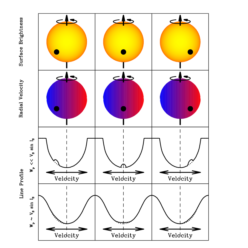
A pedagogic illustration of the physics of the Rossiter-McLaughlin effect is presented in Figure 1. The top row of panels illustrates the progress of a transiting planet across the limb-darkened disk of its parent star. This is the origin of the photometric signal. In the second row of panels, the stellar disk has been color-coded according to the local line-of-sight velocity due to rotation. One half is blueshifted, and the other half is redshifted. This is the origin of the RM signal. The third row of panels is a schematic view of a stellar absorption line that would be recorded in unresolved (i.e., disk-integrated) observations, for the case in which rotation is the dominant source of line broadening. The planet hides a small fraction of a small range of velocity components. The result is a “bump” that moves through spectral line as the planet moves across the star. The idea is essentially the same one that is employed in Doppler imaging of rapidly rotating stars (see, e.g., Rice 2002), except in this case the contrast is provided by an opaque foreground object rather than star spots. The final row of panels depicts the case in which rotation is not the dominant source of broadening. The distortion in this case is most easily detected as a net Doppler shift.

Figure 1.— The physics of the RM effect. Top row. Three successive phases of an exoplanetary transit. Second row. Same, but the projected stellar rotation speed at each point has been color coded, neglecting differential rotation. At each phase, the planet hides a different velocity component. Third row. Illustration of an observed stellar absorption line, for the case of purely rotational broadening, i.e., the net broadening due to all other mechanisms is much less than the rotational broadening ($W_{p}\ll V_{S}\sin I_{S}$). The missing velocity component is manifested as a time-variable bump in the line profile. Fourth row. Same, but for the case $W_{p}\sim V_{S}\sin I_{S}$, in which other line-broadening mechanisms besides rotation are important.

Most of the known exoplanets have been discovered by searching for periodic Doppler shifts in the spectrum of a star that result from the star’s reflex velocity (i.e., its orbital motion around the star-planet center of mass). The target stars in these searches are deliberately chosen to be inactive main-sequence FGK stars, which by nature are slow rotators ($\lower 2.15277pt\hbox{$\;\buildrel<\over{\sim}\;$}5$ km s^-1). The reason is that those stars offer the smallest intrinsic velocity noise. This means that the RM effect is appropriately described as an anomalous radial velocity. When a spectrum taken during transit is compared with a standard stellar template in order to measure the radial velocity shift, the distortion of the spectral lines will induce a signal which appears as an anomalous radial velocity.

How can the size of the anomalous velocity be predicted, in terms of the planetary and stellar properties? If, for example, the observed spectrum is simply cross-correlated with a standard stellar template, then there would be a wavelength shift in the peak of the cross-correlation function relative to the unocculted case. In this case, an excellent approximation for the velocity anomaly can be obtained by computing the first moment of the distorted line profile (i.e., the flux-weighted mean wavelength), and comparing it to the first moment of the line profile in the out-of-transit spectrum, as was done by Ohta et al. (2005) and Gimenez (2006).

In fact, as discussed by Winn et al. (2005), the accuracy of this approximation depends on the exact procedure by which radial velocities are extracted from a series of observed spectra. For example, Butler et al. (1996) use a procedure that is optimized for high precision velocity measurements using an iodine reference cell. It is considerably more complicated than a simple cross-correlation, and has as its working assumption that all spectral changes are due only to an overall Doppler shift (which is to be measured) and variations in the focus or the instrument. Winn et al. (2005) gave evidence that in this case the first-moment approximation for the RM effect is only accurate to within $\sim$10% for HD 209458. This level of accuracy is sufficient for our main purpose of providing scaling relations and estimated measurement accuracies within a factor of 2. For this reason, we will employ the first-moment approximation throughout this paper. However, it is interesting to note that the reported size of the anomaly will depend on the precise method by which radial velocities are extracted, which may make it difficult to compare the results of different investigators even when they observe the same system.

Consider a star with mass $M$ and radius $R$ that has a transiting planet with mass $m$ and radius $r$. The orbit has a period $P$, eccentricity $e$, and argument of pericenter $\omega$. We can write the net radial velocity variation of the star ($\Delta V$) as the sum of the radial velocity of the star due to its orbital motion ($\Delta V_{O}$) and the anomalous radial velocity due to the RM effect ($\Delta V_{R}$):

$$\Delta V(t)=\Delta V_{O}(t)+\Delta V_{R}(t).$$ (1)

The “O” stands for orbit, and the “R” refers to both Rossiter-McLaughlin and rotation.

The line-of-sight component of the orbital velocity is

$$\Delta V_{O}(t)=K_{O}\left\{\cos[f(t)+\omega]+e\cos\omega\right\},$$ (2)

where $f$ is the true anomaly and $K_{O}$ is the orbital velocity semiamplitude,

$$K_{O}=\left(\frac{2\pi G}{P}\right)^{1/3}\frac{m\sin I}{(M+m)^{2/3}}\left(1-e^{2}\right)^{-1/2}$$ (3)

$$=8.9~{}{\rm cm\,s^{-1}}\left(\frac{P}{{\rm yr}}\right)^{-1/3}\left(\frac{m\sin i}{M_{\oplus}}\right)\left(\frac{M}{M_{\odot}}\right)^{-2/3},$$

where $I$ is the orbital inclination with respect to the sky plane. In the latter equality we have assumed $m\ll M$ and $e=0$.

Assuming that the width of the absorption line is dominated by rotational broadening, and further assuming that the stellar Doppler shift is small, the first-moment approximation mentioned previously gives (Ohta et al., 2005):

$$\Delta V_{R}(t)=-V_{S}\sin I_{S}\frac{\int\int x{\cal I}(x,y)dxdy}{\int\int{\cal I}(x,y)dxdy}.$$ (4)

Here, $V_{S}$ is the equatorial rotation speed of the stellar photosphere, $I_{S}$ is the inclination of the stellar spin axis relative to the sky plane, and ${\cal I}(x,y)$ is the surface brightness of the observed stellar disk (including the dark spot due to the planet). The sky-plane coordinates $x$ and $y$ are measured in units of the stellar radius, have their origin at the projected center of the star, and are perpendicular and parallel to the projected stellar rotation axis, respectively. In fact, equation (4) also holds for lines that have additional broadening mechanisms, such as thermal broadening, provided that the additional broadening mechanisms produce no net Doppler shift (i.e., the broadening kernel is symmetric about its centroid).

For convenience, we write the RM effect as

$$\Delta V_{R}(t)=K_{R}~{}g(t;x_{p},y_{p},\gamma,\epsilon,...),$$ (5)

separating the overall amplitude $K_{R}$ of the RM effect from the dimensionless function $g(t)~{}\lesssim~{}1$. The amplitude is given by

$$K_{R}\equiv V_{S}\sin I_{S}~{}\frac{\gamma^{2}}{1-\gamma^{2}},$$ (6)

$$=52.8~{}{\rm m\,s^{-1}}\left(\frac{V_{S}\sin I_{S}}{5~{}{\rm km\,s^{-1}}}\right)\left(\frac{r}{R_{\rm Jup}}\right)^{2}\left(\frac{R}{R_{\odot}}\right)^{-2}$$

where $\gamma\equiv r/R$. In the latter equality, we have assumed $\gamma\ll 1$. For convenience, we will define $V\equiv V_{S}\sin I_{S}$. The dimensionless function $g$ depends primarily on the projected position of the planet $(x_{p},y_{p})$, but also on $\gamma$ and the limb-darkening function. For simplicity, we use a single-parameter “linear” description of the limb darkening law, such that the (unocculted) surface brightness of the star is

$$\frac{{\cal I}(x,y)}{{\cal I}_{0}}=1-\epsilon\left[1-\left(1-x^{2}-y^{2}\right)^{1/2}\right],$$ (7)

with $\epsilon$ the linear limb darkening parameter. Note that in some circumstances—for example, the case of differential rotation as discussed in §3—the function $g$ will depend on additional parameters.

Figure 2 shows three different trajectories of a transiting planet across the stellar disk. These trajectories all have the same impact parameter $b$, and consequently they all produce exactly the same photometric signal. However, the trajectories differ in the value of $\lambda$, and consequently produce different RM waveforms, as plotted in the lower row of panels. The sensitivity of the RM waveform to $\lambda$ is what enables the observer to assess spin-orbit alignment. The question of the achievable accuracy in $\lambda$ will be taken up in the next section.

Figure 2.— The dependence of the RM waveform on $\lambda$. Three different possible trajectories of a transiting planet are shown, along with the corresponding RM waveform (as computed with the formulae of Ohta et al. 2005). The trajectories all have the same impact parameter and produce the same light curve, but they differ in $\lambda$ and produce different RM curves. The dotted lines are for the case of no limb darkening ($\epsilon=0$), and the solid lines are for $\epsilon=0.6$.

An especially simple case is when the planetary disk is fully contained within the stellar disk, and limb darkening is negligible ($\epsilon=0$). In that case, $g$ is the perpendicular distance from the projected stellar spin axis, $g(t)=x_{p}(t)$. If we consider a rectilinear trajectory across the face of the star with impact parameter $b$, we can write the position of the center of the planet as a function of time as,

$$x_{p}(t) = \tau\cos\lambda-b\sin\lambda,$$

$$y_{p}(t) = \tau\sin\lambda+b\cos\lambda,$$ (8)

where $\tau\equiv(t-t_{\rm tra})/T_{\rm tra}$, $t_{\rm tra}$ is the time of the transit midpoint, $T_{\rm tra}=R/v_{\rm orb}$ is the radius crossing time corresponding to the planet’s orbital velocity at the time of transit (so that the transit duration is approximately $2T_{tra}\sqrt{1-b^{2}}$) and $\lambda$ is the angle of the trajectory with respect to the the apparent stellar equator. We define $\lambda$ to be between $-180\arcdeg$ and $+180\arcdeg$, such that for $\lambda>0$, the planet moves towards the stellar north pole as it proceeds across the stellar disk. We note that due to the rotation of the star, the familiar symmetry $b\leftrightarrow-b$ of the photometric signal is broken, and thus it is important to specify the sign of $b$ when considering the RM effect.

From equation (8), it is clear that in the case of uniform rotation, no limb-darkening, and when the planet is fully contained within the stellar disk, the RM curve is simply a linear function of time. During ingress and egress, and when limb darkening is taken into account, the expression for $g$ is more complicated and may need to be evaluated numerically. However, Ohta et al. (2005) and Gimenez (2006) provide useful approximate analytic expressions.

For our order-of-magnitude calculations, we will assume that the planet is small ($\gamma\ll 1$), and we will not be concerned with the ingress and egress phases because they constitute only a small fraction ($\sim$2$\gamma$) of the entire duration of the transit. For now, we will also neglect limb darkening. We therefore adopt the simple approximation

$$g(t)=\left\{\begin{array}[]{ll}x_{p}(t)&{\rm if}\,\,\sqrt{\tau^{2}+b^{2}}\leq 1,\\ 0&{\rm otherwise}.\end{array}\right.$$ (9)

It is interesting to compare the amplitude of the stellar orbital velocity $K_{O}$ with the amplitude of the anomalous velocity $K_{R}$. Assuming circular orbits ($e=0$), $\gamma\ll 1$, and $I=90^{\circ}$, we find

$$\frac{K_{R}}{K_{O}}=\left(\frac{PV^{3}}{2\pi Gm}\right)^{1/3}\left(\frac{\rho_{*}}{\rho_{p}}\right)^{2/3},$$ (10)

where $\rho_{p}$ and $\rho_{*}$ are the average densities of the planet and star, respectively. Since we expect $\rho_{*}/\rho_{p}$ to vary by no more than a factor of a few from system to system, the order of magnitude of $K_{R}/K_{O}$ depends mainly on the orbital period, the mass of the planet, and the projected rotation speed of the star. We find

$$\frac{K_{R}}{K_{O}}\sim 0.3\left(\frac{m}{M_{\rm Jup}}\right)^{-1/3}\left(\frac{P}{3~{}{\rm days}}\right)^{1/3}\left(\frac{V}{5~{}{\rm km\,s^{-1}}}\right)$$ (11)

All of the currently-known transiting exoplanets have masses that are comparable to Jupiter’s mass, and orbital periods of 1–4 days. For these systems, the anomalous velocity is smaller than the orbital velocity by a factor of a few. However, the properties of the known systems have been subject to very strong selection effects: the transits of large, short-period planets are much easier to detect than those of small, long-period planets (Gaudi 2005, Gaudi et al. 2005). An interesting implication of equation (11) is that for the most challenging systems (small planets, long periods), the amplitude of the RM effect will exceed the stellar orbital velocity. In particular, for an Earth-mass planet with a period of one year, $K_{R}/K_{O}\sim 3$ for $V=5~{}{\rm km\,s^{-1}}$. This explains the appealing possibility of using the RM effect to detect or confirm transits, which will be discussed further in § 5.

3. Prospects for Measuring Spin-Orbit Alignment

In this section, we consider what can be learned from observations of the RM effect in the regime of large $S/N$. We have in mind high-cadence, high-precision observations of both the photometric and spectroscopic transit by a hot Jupiter, for which the spectroscopic orbit is already well established.

As mentioned in § 1, a principal goal of such studies is the determination of $\lambda$, the angle on the sky between the stellar spin axis and the planetary orbit normal, because this angle gives a lower bound on any misalignment between the angular momenta of the star and the orbit. The value of $\lambda$ is determined or bounded by fitting a parameterized model to the photometric and spectroscopic measurements (see, e.g., Winn et al. 2005 and Wolf et al. 2006). However, for simple calculations, and for planning purposes, it is useful to have some heuristics and order-of-magnitude estimates for the effect of $\lambda$ on the RM waveform.

In particular, it is useful to consider the relative timing of three observable events: the moment of greatest transit depth ($t_{\rm tra}$); the moment when the orbital radial velocity variation is zero ($t_{\rm orb}$); and the moment when the anomalous RM velocity variation is zero ($t_{\rm rot}$). At $t=t_{\rm tra}$, the projected planet-star distance is smallest. At $t=t_{\rm orb}$, the star is moving in the plane of the sky. At $t=t_{\rm rot}$, the planet lies directly in front of the stellar rotation axis. For a circular orbit with $\lambda=0$, these three events are simultaneous. If the orbit is circular but $\lambda\neq 0$, then $t_{\rm tra}=t_{\rm orb}$ but $t_{\rm rot}$ will occur either earlier or later:

$$\frac{t_{\rm rot}-t_{\rm tra}}{T_{\rm tra}}\approx b\tan\lambda.$$ (12)

This is easily derived from equation (8). For a noncircular orbit, $t_{\rm tra}$ and $t_{\rm orb}$ are no longer simultaneous. To first order in $e$,

$$t_{\rm orb}-t_{\rm tra}=\frac{P}{2\pi}\left(e\cos\omega\right),$$ (13)

where $\omega$ is the argument of pericenter. To the same order, both the time difference $t_{\rm rot}-t_{\rm tra}$ and the transit duration $T_{\rm tra}$ are multiplied by the same factor $1-e\sin\omega$, and hence Eq. 12 remains valid. These expressions give some sense of the timing accuracy that is needed for a desired accuracy in $\lambda$. For example, for a mid-latitude transit at $b=0.5$ lasting 2.5 hr, a misalignment of $\lambda=1\arcdeg$ corresponds to a timing offset of 45 seconds between the transit midpoint and the null in the RM waveform.

Next, we derive an expression for the expected uncertainty in $\lambda$ based on a series of spectroscopic measurements. Consider a series of $N$ radial velocity measurements taken at times $t_{k}$ during the planetary transit (between first and fourth contact), each of which has an uncertainty $\sigma$. We consider the case in which the RM measurements are the limiting source of error; we assume that both the photometric transit and the spectroscopic orbit have already been measured accurately. Thus the times of contact, $t_{\rm tra}$, and the parameters $\gamma$ and $b$ have negligible uncertainties, and the orbital velocity $\Delta V_{O}(t)$ can be accurately subtracted from the total velocity variation observed during transits to isolate the RM waveform. The only parameters to be determined by fitting the transit data are $\lambda$ and $V$, which we combine into a two-dimensional parameter vector $\vec{a}$. The expected uncertainties in $\lambda$ and $V$ are the square roots of the diagonal elements of a matrix $C$ that is given by

$$C=B^{-1},$$ (14)

where $B$ is related to the Fisher information matrix (see Gould 2003) and is calculated as

$$B_{ij}\equiv\sum_{k=1}^{N}\frac{1}{\sigma^{2}}\left[\frac{\partial}{\partial a_{i}}\Delta V_{R}(t_{k})\right]\left[\frac{\partial}{\partial a_{j}}\Delta V_{R}(t_{k})\right].$$ (15)

We will adopt the approximate analytic form for $\Delta V_{R}(t)$ that was given in equation (9). Assuming evenly-spaced observations and large $N$, we can convert the sum in equation (15) into an integral. This then yields the following expressions for the expected uncertainties in $\lambda$ and $V$:

$$\sigma_{\lambda}=Q_{R}^{-1}\left[\frac{(1-b^{2})\sin^{2}{\lambda}+3b^{2}\cos^{2}{\lambda}}{b^{2}(1-b^{2})}\right]^{1/2},$$ (16)

$$\frac{\sigma_{V}}{V}=Q_{R}^{-1}\left[\frac{(1-b^{2})\cos^{2}{\lambda}+3b^{2}\sin^{2}{\lambda}}{b^{2}(1-b^{2})}\right]^{1/2},$$ (17)

where we have defined

$$Q_{R}\equiv\sqrt{N}\frac{K_{R}}{\sigma}.$$ (18)

As discussed further in §5, the factor $Q_{R}$ is proportional to the total signal-to-noise ratio of the measured RM waveform. Note that $\sigma_{V}(\lambda)/V=\sigma_{\lambda}(\pi-\lambda)$. Similarly, we can derive the covariance between $\lambda$ and $V$, which is given by ${\rm cov}(\lambda,V)=C_{12}/(C_{11}C_{22})^{1/2}$. We find

$${\rm cov}(\lambda,V)=\frac{4b^{2}-1}{\left[(1-b^{2})^{2}+9b^{4}+3b^{2}(1-b^{2})(\tan^{2}\lambda+\cot^{2}\lambda)\right]^{1/2}}.$$ (19)

The uncertainty in each parameter is the product of $Q_{R}^{-1}$ and a factor that depends on the orbital geometry. The geometrical factor is illustrated in Figure 3, for $\gamma=0.1$ and three values of the impact parameter $b$. The solid lines show the expected uncertainties in $\lambda$ and $V$ given by equations (16) and (17), after dividing by $Q_{R}^{-1}$. The three cases are a near-central transit ($b=0.1$), a mid-level transit ($b=0.5$), and a grazing transit ($b=0.9$). For $b=0.5$, we find that $\sigma_{\lambda}=\sigma_{V}/V=2Q_{R}^{-1}$, and that the uncertainties in $V$ and $\lambda$ are uncorrelated [${\rm cov}(\lambda,V)=0$]. In this sense, mid-level transits are ideal for cleanly separating the effects of $V_{S}\sin I_{S}$ and $\lambda$ on the RM waveform.

In contrast, for nearly central transits there is a strong degeneracy between $\lambda$ and $V$ and a strong dependence of $\sigma_{\lambda}$ on $\lambda$. For $b=0$ exactly, ${\rm cov}(\lambda,V)=-1$. The observed signal depends only on the parameter combination $V\cos{\lambda}$, and the timing offset given in Eq. (13) is zero regardless of $\lambda$. One can measure only the amplitude of the RM waveform, and cannot tell whether a small amplitude (say) is the result of an equatorial transit across a slowly rotating star, or a misaligned transit across a more rapid rotator. An accurate measurement and interpretation of the line broadening in the out-of-transit spectra is essential here, by providing an independent estimate of $V$ that can be used as an a priori constraint. For grazing transits, there is a more modest dependence of the uncertainties on $\lambda$ (although our approximations are least accurate for grazing transits, as described below).

In order to verify our analytic expressions, and evaluate the importance of some of the effects that these expressions neglect (namely, the finite ingress/egress durations and limb darkening), we numerically evaluated the elements of the Fisher matrix $B$ using the more accurate but more complex expressions for $\Delta V_{R}(t)$ given by Ohta et al. (2005). The results are also plotted in Figure 3. The dotted lines show the results for $\epsilon=0$ (no limb darkening), and the dashed lines show the results for $\epsilon=0.6$. Except for non-grazing transits, the differences between the uncertainties predicted by our analytic expressions and the numerically-calculated uncertainties are small ($\lesssim 10\%$). Not surprisingly, for grazing transits the differences are substantially larger and can be a factor of 2.

Next, we verified our results using Monte Carlo simulations. For a given choice of $V$ and $\lambda$, we created $5000$ simulated data sets of radial velocity measurements during a transit. Each data point was the value calculated according to the expressions of Ohta et al. (2005), plus Gaussian noise with a standard deviation of $\sigma$. We then used a downhill-simplex algorithm to optimize the parameter values $V$ and $\lambda$ for each data set. We calculated the dispersions in the resulting distribution of 5000 fitted values, and took the dispersion to be the uncertainty in that parameter. We repeated this procedure for a range of $V$ and $\lambda$. The resulting uncertainties agree very well with the uncertainties computed by numerically evaluating the elements of $B$ as described above.

We now consider the 5 particular cases of known transiting exoplanets with bright ($V<12$) parent stars: HD 209458 (Henry et al. 2000, Charbonneau et al. 2000), TrES-1 (Alonso et al. 2004), HD 189733 (Bouchy et al., 2005c), HD 149026 (Sato et al. 2005), and XO-1 (McCullough et al. 2006). For the systems for which the RM effect has already been measured, this exercise provides an empirical check on our calculations. For the others, it provides a guide for the achievable accuracy of future observations. Below we describe our assumptions and the results for each planet in detail; this information is summarized in Table 1.

For HD 209458, an analysis of the best available photometric and spectroscopic data was performed by Winn et al. (2005). The data set included $N=14$ radial velocity measurements during transits, with a typical uncertainty of $\sigma=4.1~{}{\rm m\,s^{-1}}$. By fitting a parameterized model to all of the data, and evaluating the parameter uncertainties with a Monte Carlo bootstrap technique, they found $\lambda=-4^{\circ}\hskip-4.5pt.4\pm 1^{\circ}\hskip-4.5pt.4$ and $V=4.70\pm 0.16~{}{\rm km\,s^{-1}}$. Using these values, as well as the parameters $\gamma=0.121$ and $b=0.52$ determined from the photometry, our analytic estimates predict that the uncertainties should be $\sigma_{\lambda}=1^{\circ}\hskip-4.5pt.7$ and $\sigma_{V}=0.15~{}{\rm km\,s^{-1}}$. These estimates are in excellent agreement with the actual uncertainties derived from detailed model-fitting. In addition, Eq. (19) predicts that the uncertainties in $V$ and $\lambda$ should be uncorrelated, as was indeed found to the be the case by Queloz et al. (2000) and Winn et al. (2005).

For HD 149026, Wolf et al. (2006) analyzed all of the available photometric and spectroscopic data, including $N=15$ radial velocity measurements taken during transit. The typical velocity uncertainty was $\sigma=4.0~{}{\rm m\,s^{-1}}$. Through parameterized model-fitting and bootstrap resampling, these authors found $\lambda=11^{\circ}\hskip-4.5pt\pm 14^{\circ}\hskip-4.5pt$, $V=6.4_{-0.7}^{+2.1}~{}{\rm km\,s^{-1}}$, $\gamma=0.051$, and $b=0.39$. Our analytic formulae predict $\sigma_{\lambda}=9.0^{\circ}\hskip-3.5pt$ and $\sigma_{V}=0.76~{}{\rm km\,s^{-1}}$. Our estimates are smaller than the Wolf et al. (2006) uncertainties. We believe that the reason is that the photometric signal is not nearly as well determined for HD 149026 as it is for HD 209458, not only because of the smaller size of the planet, but also because the existing observations are from ground-based telescopes as opposed to the higher-precision Hubble Space Telescope light curve obtained by Brown et al. (2001) for HD 209458. Consequently, the uncertainties in the parameters $t_{\rm tra},\gamma$, and $b$ cannot be neglected. The covariance with these photometric parameters contribute to the uncertainty in $\lambda$ and $V$, violating one of the conditions for the accuracy of our analytic estimates. We conclude that there is scope for improvement in the determination of $\lambda$ for this system through improved photometry.

As mentioned in the introduction, the transits of HD 189733b were originally discovered via the RM effect (Bouchy et al., 2005c), but those authors did not attempt to measure $\lambda$ or $V$ by fitting the RM waveform. However, using their estimate of $V=3.5\pm 1.0~{}{\rm km\,s^{-1}}$ derived from the out-of-transit spectral line profile, we can anticipate the expected uncertainties of such attempts, through an application of our expressions. The photon noise in the radial velocity measurements reported by Bouchy et al. (2005c) amounts to only $\sim$5-7 ${\rm m\,s^{-1}}$, but the actual uncertainties are larger because the star is fairly active. As an estimate of this “stellar jitter,” we will adopt the value $\sigma=15~{}{\rm m\,s^{-1}}$ based on the scatter around the Keplerian orbital solution. Taking $b=0.66$ and $\gamma=0.157$ (Bakos et al., 2006), we predict $\sigma_{\lambda}=5^{\circ}\hskip-4.5pt.2$ and $\sigma_{V}=0.48~{}{\rm km\,s^{-1}}$ for $N=8$ (again, assuming that the measurement of the RM waveform is the limiting uncertainty). These values are based on the assumption $\lambda\sim 0$, although the expected uncertainties are fairly insensitive to $\lambda$ because the transit is neither central nor grazing (see the previous section). If the velocity jitter turns out to be smaller, or if a larger number of transit velocities are measured, then the uncertainties in the RM parameters will scale as $\sigma/\sqrt{N}$.

No measurements of the RM effect have yet been reported for TrES-1 or XO-1. We estimate the accuracy with which $\lambda$ can be constrained in these systems with future observations, using the parameters of the systems that have been derived from the existing photometric and spectroscopic data. For specificity, we assume $N=15$ and $\sigma=15~{}{\rm m\,s^{-1}}$. The latter estimate for $\sigma$ seems reasonable, given that the apparent magnitudes of the host stars ($m_{V}=11-12$) are fainter than the three stars considered above ($m_{V}=8$).

For TrES-1, there exists only an upper limit on the projected stellar rotation velocity of $V\lesssim 5~{}{\rm km\,s^{-1}}$. We will optimistically assume that the true value is $5~{}{\rm km\,s^{-1}}$, right at the upper limit. Then, assuming $b=0.18$ and $\gamma=0.137$ (Alonso et al., 2004; Sozzetti et al., 2004), we find $\sigma_{\lambda}=13^{\circ}$ and $\sigma_{V}=0.36~{}{\rm km\,s^{-1}}$ for $\lambda=0$, and $\sigma_{\lambda}=4^{\circ}\hskip-4.5pt.1$ and $\sigma_{V}=~{}1.1~{}{\rm km\,s^{-1}}$ for $\lambda=90^{\circ}$. The strong sensitivity to $\lambda$ arises because the transit is nearly central.

For XO-1, we adopt $V=1.11~{}{\rm km\,s^{-1}}$, $b=0.12$ and $\gamma=0.131$ (McCullough et al., 2006; Holman et al., 2006), and find $\sigma_{\lambda}=95^{\circ}$ and $\sigma_{V}=0.39~{}{\rm km\,s^{-1}}$ for $\lambda=0$, and $\sigma_{\lambda}=20^{\circ}$ and $\sigma_{V}=1.8~{}{\rm km\,s^{-1}}$ for $\lambda=90^{\circ}$. Again, for this fairly central transit, the expected uncertainty depends strongly on $\lambda$.

For both TrES-1 and XO-1b the uncertainties in $\lambda$ and $V$ are expected to be fairly large unless a substantial commitment of resources are expended to acquire many high-$S/N$ spectra during transit, or the individual velocity uncertainties can be reduced substantially below the $15~{}{\rm m\,s^{-1}}$ assumed here. This is because in both cases, the projected stellar rotation velocities are fairly small, and the transits are nearly central (small $b$). This gives rise to large uncertainties in $V$ (for $\lambda\sim 0$) or $\lambda$ (for $\lambda\sim 90^{\circ}$).

Table 1Predictions for Rossiter-McLaughlin Effect Parameter Uncertainties

Name	$N$	$\sigma$	$\gamma$	$b$	$V$	$\lambda$	$K_{R}$	$\sigma_{\lambda}$	$\sigma_{V}$
		${\rm m\,s^{-1}}$			${\rm km\,s^{-1}}$	deg	${\rm m\,s^{-1}}$	deg	${\rm km\,s^{-1}}$
HD 209456b	14	4.1	0.121	0.52	4.70	$-4.4$	70	1.7	0.15
HD 149026b	15	4.0	0.051	0.39	6.4	11	17	9.0	0.76
HD 189733b	8	15	0.157	0.66	3.5	0	88	5.2	0.48
–	–	–	–	–	–	90	–	7.9	0.32
TrES-1b	15	15	0.137	0.18	5	0	96	13	0.36
–	–	–	–	–	–	90	–	4.1	1.1
XO-1b	15	15	0.131	0.12	1.11	0	19	95	0.39
–	–	–	–	–	–	90	–	20	1.8

Note. — For HD 189733b, a fit to the Rossiter-McLaughlin effect data has not been reported, and so no constraint on $\lambda$ is available. We therefore show the expected parameter uncertainties for the two values $\lambda=0,90^{\circ}$, which will bracket the range of uncertainties. For TrES-1b and XO-1b, no Rossiter-McLaughlin data has been reported, and so we assume $N=15$, $\sigma=15~{}{\rm m\,s^{-1}}$, and show the expected parameter uncertainties for the two values $\lambda=0,90^{\circ}$.

Figure 3.— The achievable total signal-to-noise ratio in RM waveform (left), and the signal-to-noise ratio in the the RM parameters $\lambda$ and $V$ (right), as a function of $b$ and $\lambda$. Plotted is the “normalized” signal-to-noise ratio (i.e., after dividing by $Q_{R}$; see Eq. 18) for $\lambda$ (black lines) and for $V$ (gray lines). The solid lines are based on our analytic formulae. The dotted and dashed lines are based on numerical computations with the more accurate formulas of Ohta et al. (2005); the dotted lines are for the case of no limb darkening, and the dashed lines are for linear limb darkening with $\epsilon=0.6$.

In addition to these 5 systems, there are 5 other known transiting planets, all of which were originally identified as candidates by the OGLE collaboration (Udalski et al., 2002a, b, c, 2003), and subsequently confirmed with radial velocity follow-up (Konacki et al., 2003a, b; Konacki et al., 2004, 2005; Bouchy et al., 2004; Pont et al., 2004; Moutou et al., 2004; Pont et al., 2005; Bouchy et al., 2005a). The stars in these systems are all fainter than the five cases considered above ($m_{V}\simeq 15.5-17$ versus $m_{V}\simeq 8-12$), which will make the measurement of the RM effect much more challenging for these systems. Nevertheless, there is a good reason to expend this additional effort on at least some of the OGLE systems, namely, the “very hot Jupiters” (VHJs) with orbital periods less than 3 days. It has been suggested that these shorter-period planets discovered by OGLE form a distinct population from the more numerous “hot Jupiters” with 3-4 day periods, based on differences in their typical mass (Gaudi et al., 2005; Mazeh et al., 2005) and their overall frequency (Gaudi et al., 2005; Gould et al., 2006). This raises the interesting possibility that the VHJs arrived at their very close orbits through a different mechanism than the hot Jupiters. For example, the observation that the orbital distances of VHJs are nearly equal to twice their Roche radii (Ford & Rasio, 2006) may indicate that these planets were emplaced via tidal capture and subsequent circularization. Such a scenario would be the natural result of planet-planet scattering (Rasio & Ford, 1996; Ford et al., 2001), capture of free-floating planets (Gaudi, 2003), or Kozai oscillations (Wu & Murray 2003, D. Fabrycky & S. Tremaine, priv. comm.). In the latter two scenarios, at least, one would expect these planets to generically have orbits with large misalignments with the spin axis of their parent stars.

We can repeat our previous analysis to estimate the achievable uncertainty in $\lambda$ for the OGLE systems. Unfortunately, many of the parameters needed to provide an accurate estimate (particularly the impact parameter $b$ and projected stellar rotation speed $V$) have not been measured, or have substantial uncertainties. We will therefore adopt approximate, fiducial values in order to provide an order-of-magnitude estimate, with the caution that the actual uncertainties could be significantly different. We will assume $b=0.5$, $\gamma=0.1$ and $\epsilon=0.6$. Only upper limits for the rotational velocities of the host stars have been reported, so we will adopt the largest allowed velocity of $V=5~{}{\rm km\,s^{-1}}$. Typical radial velocity precisions reported for these systems are $\sigma\simeq 50~{}{\rm m\,s^{-1}}$ for $\sim 45~{}{\rm minute}$ exposures (using 10m-class telescopes), which we scale to $\simeq 100~{}{\rm m\,s^{-1}}$ for $10$-minute exposures. Assuming continuous observations during a typical transit duration of $\sim$2 hr (i.e., twelve $10$-minute exposures), we find $Q_{R}\simeq 1.7$ per transit, and so $\sigma_{\lambda}=2Q_{R}^{-1}\sim 70^{\circ}$. With observations of 4 transits, one could measure $\lambda$ to within about $35^{\circ}$. While this is not nearly as good as the results that can be achieved for the systems with brighter host stars, even the finding that one of the VHJs has (say) $\lambda=-90^{\circ}\pm 35^{\circ}$ would be quite interesting.

4. Differential Rotation

In the preceding calculations we neglected differential rotation, i.e., we assumed that the rotation speed of the star was independent of the stellar latitude. One might wonder whether or not the expected degree of differential rotation is detectable through transit observations. If so, it would be important both as a stellar astrophysics tool, and (if it is not modeled properly) as a possible source of ambiguity or covariance in the interpretation of RM data.

Differential rotation is an important phenomenon in stellar astrophysics because it is an observable manifestation of convective dynamics, and because it is intimately linked to the dynamo mechanism of stellar magnetic field generation and evolution. The Sun rotates $\sim$20% faster at its equator than at high latitudes (see, e.g., Howard 1984 and references therein). Differential rotation has also been measured for other stars using star spots. In some cases, spots at different latitudes produce measurably different photometric periods (see, e.g., Henry et al. 1995, Rucinski et al. 2004, Herbst et al. 2006), and in other cases, the motion of star spots has been tracked via Doppler imaging (Collier Cameron et al. 2002).

In principle, transiting exoplanets can be used instead of star spots. The advantages would be that planetary orbits are much more stable than star spot patterns, the transit chord can occur at any stellar latitude and can span a wide range of latitudes (unlike star spots), and the time scale of the transit (a few hours every few days) is more convenient than the month-long rotation periods of many stars. In addition, it would allow differential rotation to be measured on inactive and unspotted stars for the first time. A system of multiple transiting planets with different impact parameters has yet to be discovered, but would be a wonderful probe of differential rotation. But even with a single transiting planet, it is possible in principle to detect differential rotation through the RM effect if $\lambda\neq 0$. The RM waveform effectively traces the projected surface speed of the star along a one-dimensional chord, and is sensitive to differential rotation if the chord spans a significant range of latitude.

It is customary to parameterize observations of differential rotation according to a function such as $V(\ell)=V_{\rm eq}(1-\alpha\sin^{2}{\ell})$, where $V_{\rm eq}$ is the rotation speed at the stellar equator, $\ell$ is the latitude on the surface of the star, and $\alpha$ is the differential rotation parameter (which is equal to the fractional difference in rotation speed between the pole and the equator). For the Sun, differential rotation is significant, $\alpha=0.2$. For stars with convective envelopes ($T_{eff}\lesssim 7500~{}{\rm K}$), the amount of differential rotation is thought to be correlated with $V_{\rm eq}$, such that more rapid rotators exhibit less differential rotation (Barnes 2005, Reiners 2006). For stars lacking exterior convection zones, the surface differential rotation is small and $\alpha\sim 0$.

If the surface of the star is in uniform rotation, then the surface speed at any point on the star depends only on the projected rotation speed of the star, $V=V_{S}\sin I_{S}$, and the distance from the the projected rotation axis, $x_{p}$ (Eq. 8). However, in the case of differential rotation, this symmetry is broken. The surface speed at a given point on the star also depends on the position parallel to the projected axis $y_{p}$, as well as on the inclination of the rotation axis, $I_{S}$. The apparent rotation speed at any point $(x_{p},y_{p})$ of the stellar surface is

$$v(x_{p},y_{p})=-V_{\rm eq}\sin I_{S}~{}~{}x_{p}\left\{1-\alpha\left[y_{p}\sin{I_{S}}+(1-x_{p}^{2}-y_{p}^{2})^{1/2}\cos{I_{S}}\right]^{2}\right\}.$$ (20)

Figure 4 shows the effect of differential rotation on the RM waveform. For this illustration, we used the parameters appropriate for HD 209458 ($\gamma=0.121$, $b=0.5$, and $V_{\rm eq}=5~{}{\rm km\,s^{-1}}$) and further assumed $I_{S}=90^{\circ}$, so that the rotation axis is in the plane of the sky. We took the differential rotation parameter to be equal to the solar value of $\alpha=0.2$. Each column shows the results for a different value of $\lambda$. The top row shows the waveform itself, and the bottom row shows the difference between the waveforms with $\alpha=0$ and $\alpha=0.2$.

For $\lambda=0$ and $I_{S}=90^{\circ}$, the effect of differential rotation is degenerate with changing the value of $V_{\rm eq}$, and hence differential rotation is not measurable. However, from Figure 4 and equation (20), it is clear that for $\lambda\neq 0$ or $I_{S}\neq 90^{\circ}$, these two parameters are not degenerate, and in principle both parameters can be constrained by fitting a parameterized model to the velocity data. However, the requirement on the velocity precision is stringent. The amplitude of the deviations due to differential rotation generally scale with $\alpha$, and are only a few m s^-1 for $\alpha=0.2$.

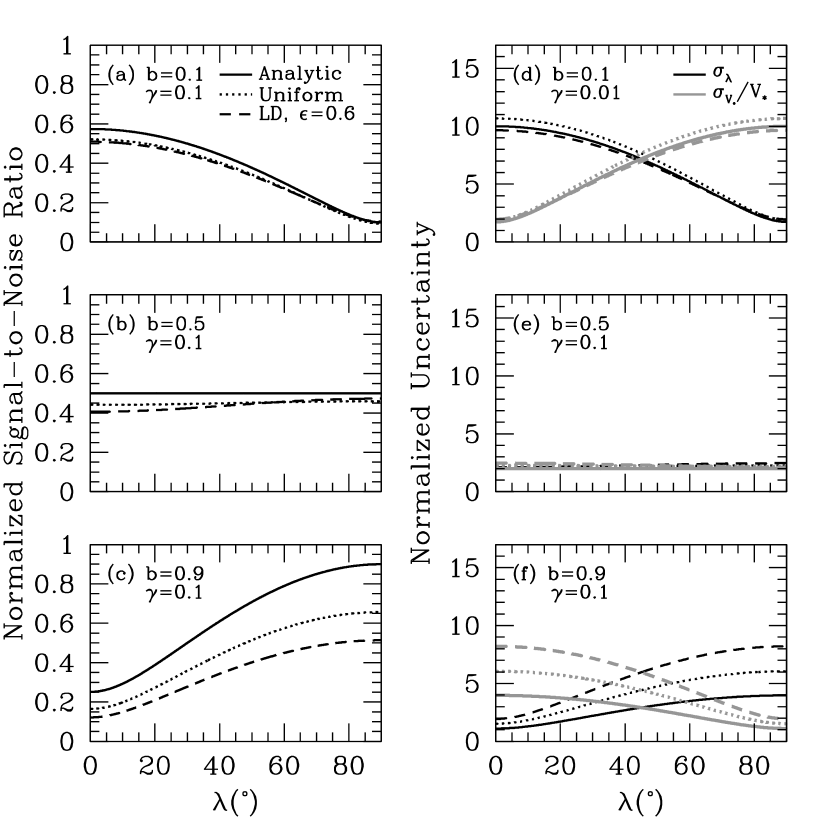
For a more quantitative analysis, we can apply the same procedure that we used in the previous section to estimate how well one can hope to estimate $\alpha$ using the RM effect. We estimate the uncertainties by numerically computing the Fisher matrix (Eq. 15) using the analytic form for the RM effect given by Ohta et al. (2005), but accounting for the effect of differential rotation on projected surface velocity (Eq. 20). We consider the uncertainties on four parameters $\vec{a}=(\lambda,v_{\rm eq},\alpha,I_{S})$, and we assume that all other parameters have negligible uncertainties. The resulting uncertainties in the parameters $\vec{a}$ exhibit complicated relationships with $\lambda$, $b$, and $I_{S}$. We will summarize our results by focusing on the case $\alpha=0.2$, $b=0.5$, $\gamma=0.121$, and $\epsilon=0.6$ (approximating the HD 209458 system). Figure 5 shows the expected uncertainties as a function of $\lambda$ for $I_{S}=30^{\circ},60^{\circ},90^{\circ}$. We show the “normalized uncertainties,” after dividing by $Q_{R}$, where $Q_{R}$ is still given by equation (18), but with a slightly altered definition of RM semiamplitude from equation (6): $K_{R}\equiv V_{\rm eq}{\gamma^{2}}/({1-\gamma^{2}})$.

Figure 4.— The spectroscopic transit in the presence of differential rotation. The top row of panels shows the expected RM waveform for a transit in a system similar to HD 209458 ($b=0.5$, $\gamma=0.121$, $V_{\rm eq}=5~{}{\rm km\,s^{-1}}$), for three different values of $\lambda$. The stellar rotation axis is taken to be in the plane of the sky, and the differential rotation parameter was set to $\alpha=0.2.$ The dotted lines show the corresponding waveforms for $\alpha=0$. The bottom row of panels show the difference between the $\alpha=0.2$ and $\alpha=0$ cases.

Figure 5.— The achievable signal-to-noise ratio in the RM and differential rotation parameters $\lambda,V_{eq},\alpha,I_{S}$, as a function of $\lambda$ for three values of $I_{S}$. We have assumed $b=0.5$, $\gamma=0.121$, and $\epsilon=0.6$, thus approximating the HD 209458 system. We have assumed differential rotation parameter equal to the solar value of $\alpha=0.2$. Plotted is the “normalized” signal-to-noise ratio (i.e., after dividing by $Q_{R}$; see Eq. 18). The solid lines show the case for no limb darkening, and the dashed lines are for linear limb darkening with $\epsilon=0.6$. The dashed lines in the top row show our analytic formula for the uncertainty in $\lambda$ in the absence of differential rotation. The difference between the dashed and solid/dotted lines demonstrates the degradation of the uncertainty in $\lambda$ due to covariance with the differential rotation parameters.

First, we consider the case in which the stellar rotation axis is in the plane of the sky: $I_{S}=90^{\circ}$ (left column of Fig. 5). As seen in Figure 4, for this case and $\lambda=0$, $\alpha$ is degenerate with $V_{\rm eq}$, and it is not possible to determine these parameters independently. In fact, for $I_{S}=90^{\circ}$ and $\lambda=0$, neither of the differential rotation parameters ($\alpha,I_{S}$) are well constrained. We find that in general the uncertainty in $\lambda$ is degraded by covariances with the other parameters (particularly $\alpha$). For example, we find $\sigma_{\lambda}\sim 3Q_{R}^{-1}$ for $\lambda\sim 0$. This is $\sim 50\%$ larger than the uncertainty expected under the assumption of solid body rotation (Eq. 16). Thus without an a priori constraint on the allowed degree of differential rotation, measurements of $\lambda$ will be significantly compromised by an unknown amount of differential rotation. We explore the effects of a constraint on $\alpha$ in more detail below.

From inspection of Figure 5, we see that for $I_{S}=90^{\circ}$, the most favorable value of $\lambda$ for measuring the overall system parameters (in the sense of minimizing the sum of the squares of the uncertainties of all four parameters) is $\lambda\approx 55^{\circ}$. For this value, we find $\sigma_{\lambda}=4.1Q_{R}^{-1}$, $\sigma_{V_{eq}}/V_{eq}=3.0Q_{R}^{-1}$, $\sigma_{\alpha}=35Q_{R}^{-1}$, and $\sigma_{I_{S}}=52Q_{R}^{-1}$. Therefore measuring $\alpha$ to within 0.2 and $I_{S}$ to within $15^{\circ}$ requires $Q_{R}\sim 200$. Achieving this high a signal-to-noise ratio for a system similar to HD 209458b would require at least $\sim$30 radial velocity measurements with uncertainties of $\sim 2~{}{\rm m\,s^{-1}}$ (although, of course, HD 209458 itself has proven to have a much smaller value of $\lambda$).

For $I_{S}=60^{\circ}$ (middle column of Fig. 5) the most favorable value is $\lambda\approx 70^{\circ}$. In this case, we find $\sigma_{\lambda}=11Q_{R}^{-1}$, $\sigma_{V_{eq}}/V_{eq}=28Q_{R}^{-1}$, $\sigma_{\alpha}=31Q_{R}^{-1}$, and $\sigma_{I_{S}}=42Q_{R}^{-1}$. The variances of the parameters are highly correlated. In particular, while the uncertainties in $V_{eq}$ and $I_{S}$ are individually high, they are correlated such that the uncertainty in $V_{eq}\sin I_{S}$ is considerably smaller. Measuring all of the parameters to better than $20\%$ will require $Q_{R}\gtrsim 200$.

We also computed the uncertainties for the same geometry as above, but for different values of $I_{S}$ and the impact parameter $b$. The right column in Figure 5 shows the results for $b=0.5$ and $I_{S}=30^{\circ}$. Generally we find that the uncertainties are relatively large for $I_{S}\lesssim 30^{\circ}$, primarily because the amplitude of the RM effect is decreased by the sky projection. Grazing transits ($b\gtrsim 0.9$) and central transits ($b\approx 0$) provide poorer constraints, but for $0.2\lesssim b\lesssim 0.7$, the uncertainties are relatively insensitive to $b$.

We conclude that, for favorable geometries ($30^{\circ}\lesssim\lambda\lesssim 70^{\circ}$ and $0.2\lesssim b\lesssim 0.7$), it may be possible to detect differential rotation and to constrain $\alpha$ and $I_{S}$ to within $\sim$20%, using very high signal-to-noise ratio observations of the RM effect ($Q_{R}\gtrsim 10^{2}$).

On the other hand, for lower signal-to-noise ratio observations, we have shown that the covariances with the differential rotation parameters (particularly $\alpha$) will degrade the measurement of $\lambda$. It is is therefore of interest to ask to what degree a modest a priori constraint on $\alpha$ will improve the expected uncertainties on $\lambda$. Because such constraints are not easily incorporated into the Fisher matrix formalism, we instead determine the uncertainties using Monte Carlo simulations, as described in §3. We first compute the expected uncertainties on the parameters with no constraints, and so verify our estimates based on the Fisher matrix formalism.

Again adopting the parameters of the HD 209458b system ($b=0.52$, $\gamma=0.121$, $\epsilon=0.6$, $\lambda=-4^{\circ}\hskip-4.5pt.4$, $V_{eq}\sin I_{S}=4.70~{}{\rm km\,s^{-1}}$, $N=14$, and $\sigma=4.1~{}{\rm m\,s^{-1}}$), we find $\sigma_{\lambda}=2^{\circ}\hskip-4.5pt.7$ for $\alpha=0.2$ (with a very weak dependence on $I_{S}$). We then enforce a weak constraint on $\alpha$ by adding a penalty term to $\chi^{2}$, of the form $\Delta\chi^{2}=[(\alpha-0.2)/0.4]^{2}$. We find $\sigma_{\lambda}=2^{\circ}\hskip-4.5pt.0$, also with a weak dependence on $I_{S}$. Thus, this mild a priori constraint reduces the expected uncertainty in $\lambda$ from a level that is 60% larger than the expectation under the assumption of solid-body rotation, to a level that is only 20% larger. At higher signal-to-noise ratios, the constraint on $\alpha$ has little effect.

5. Confirming Transiting Planets

In this section we move from the regime of high $S/N$ to the regime of low $S/N$, and investigate the utility of the RM effect in confirming the occurrence of transits in the most challenging cases. The photometric detection of transits offers one of the most promising ways to achieve the appealing goal of detecting terrestrial planets in the habitable zones of solar-type stars. That said, the challenges of robust detection of the photometric signal are daunting. A transiting Earth-sized planet orbiting in the habitable zone of a solar-type star would reduce the stellar flux by only $\sim$10^-4, for a duration of only $\sim$13 hr out of the year. Furthermore, the probability that a randomly oriented orbital plane happens to be close enough to edge-on to allow transits is only $\sim$0.5%. The requirements for detecting these signals have convinced most researchers that it is necessary to conduct the search with space telescopes rather than ground-based telescopes. Several satellite experiments are slated for launch over the next few years that are designed to survey $10^{4}-10^{5}$ main-sequence stars in order detect small transiting planets, including Corot (Baglin, 2003) and Kepler (Borucki et al., 2003).

Figure 6.— Simulated spectroscopic signal of a transiting terrestrial planet in the habitable zone a solar-type star. The line-of-sight component of the stellar orbital velocity is visible as the sinusoid with a period of one year. The RM effect is visible as the spike at the origin, which is the time of transit. A close-up of the transit interval is shown in the lower panel. We have assumed $b=0$, $\lambda=0$, $\epsilon=0.6$, $M=M_{\odot}$, $R=R_{\odot}$, $r=R_{\oplus}$, $m=M_{\oplus}$, $e=0$, $P=1$ yr, and $V=5~{}{\rm km\,s^{-1}}$.

Figure 7.— Confirmation of Kepler planets. The symbols show the masses (or minimum masses) of known exoplanets versus their orbital semimajor axes. The black triangles are planets detected via spectroscopic orbits, red stars via transits, grey hexagons via pulsar timing, and purple circles via microlensing. Also shown are the Solar system planets. The green shaded region is where Kepler can detect (with $S/N\geq 8$) at least two transits by a planet orbiting a star with apparent magnitude $m_{V}=12$. The lines show the lower mass limits of planets detectable by Kepler that can be confirmed (with $S/N\geq 5$) via spectroscopic measurement of the stellar orbital over the course of a full period (red lines) and via measurements of the Rossiter-McLaughlin effect throughout a single transit (blue lines). We show these limits based on the capability of current instruments such as HARPS (solid lines), and the expected capability of a future 30m telescope (dashed lines). For this figure, we have assumed that the host star has the mass and radius of the Sun, that its projected rotation speed is $5~{}{{\rm km\,s^{-1}}}$, and that all planets have the same mean density. Confirmation via the orbital velocity gives a lower mass limit in all cases, but it requires $\sim$10 times more observing time, and greater instrumental stability (the spectroscopic orbit occurs over a full orbital period, as opposed to a single transit).

As with many such experiments, the most exciting discoveries from these surveys are likely to be those that are detected with the lowest signal-to-noise ratio ($S/N$). Furthermore, the scaling of the number of detections as a function of the limiting $(S/N)_{\rm min}$ is generally quite steep. For example, Gould et al. (2004) demonstrated that the number of expected detections for Kepler scales as $(S/N)^{-2.4}_{\rm min}$. This implies that the number of detections is fairly sensitive to unanticipated degradations in $(S/N)_{\rm min}$ (from unexpected noise sources or other problems), and that the majority of the detections will occur very near the limiting $(S/N)_{\rm min}$. Since the limiting value of $(S/N)_{\rm min}$ will generally be the minimum possible $S/N$ for which detection is statistically possible, it will be difficult or impossible to use any further characteristics of the transit light curves themselves to distinguish true planets from false positives. If all of the information is required for mere detection, then there is not enough information for the accurate determination of multiple parameters.

Therefore, it will be essential to verify the low $S/N$ candidates with additional observations. Unfortunately, since the photometric noise requirements are so stringent, it may prove very difficult to confirm these candidates with ground-based photometric observations. Space-based satellites such as HST or JWST (Charbonneau et al., 2004; Gould et al., 2004) may deliver the sensitivity and precision to confirm these detections, provided they are available. However, it would certainly be more expedient to have a good ground-based method to confirm candidates.

The most desirable type of confirmation would be the spectroscopic detection of the stellar orbital velocity. This could be done from the ground, and the Doppler signal would also provide an estimate of the mass of the planet, and hence its mean density (when combined with the radius measurement from the photometric transit). The difficulty with the detection of the spectroscopic orbit is that the stellar reflex velocity would be quite small: the aforementioned Earth-like planet in the habitable zone of a solar-type star produces a $\sim$9 cm s^-1 wobble. Furthermore, the parent stars will be relatively faint (with an apparent magnitude $m_{V}\sim 12$ for Kepler), owing to the narrow-field, magnitude-limited design of the survey observations.

Can current setups detect the spectroscopic orbits of the systems with habitable planets that will be detected by Kepler? Before answering this question, we first estimate the parameters of the planets that can be detected with Kepler. The signal-to-noise ratio of a transiting planet with a semimajor axis $a$ and radius $r$ orbiting a star with a radius of $R$ is

$$\left(\frac{S}{N}\right)_{T}\simeq(\Gamma T)^{-1/2}\left(\frac{R}{\pi a}\right)^{1/2}\left(1-b^{2}\right)^{1/4}\left(\frac{r}{R}\right)^{2},$$ (21)

where $\Gamma T$ is the total number of photons collected from a star of the appropriate apparent magnitude during the mission lifetime $T$. For the parameters of the Kepler mission, we find

$$\left(\frac{S}{N}\right)_{T}\sim 11\left(\frac{a}{{\rm AU}}\right)^{-1/2}\left(\frac{m}{M_{\oplus}}\right)^{2/3}\left(\frac{1-b^{2}}{0.75}\right)^{1/4}10^{-0.2(m_{V}-12)},$$ (22)

where we have assumed that $R=R_{\odot}$ and that the planet has the same density as Earth: $r=R_{\oplus}(m/M_{\oplus})^{1/3}$.

We now estimate the signal-to-noise ratio with which follow-up radial velocity measurements can confirm the Kepler detections. Assuming a circular orbit, and $N_{O}$ radial velocity measurements are made with an uncertainty of $\sigma$ evenly sampled in orbital phase, then the total $S/N$ of the orbital velocity signal is

$$\left(\frac{S}{N}\right)_{O}=\frac{Q_{O}}{\sqrt{2}},$$ (23)

where we have defined

$$Q_{O}\equiv\sqrt{N_{O}}\frac{K_{O}}{\sigma}.$$ (24)

The HARPS spectrograph (Pepe et al., 2002) mounted on the 3.6m ESO telescope is representative of the state of the art in precision radial-velocity measurements. Lovis et al. (2005) discuss observations of three dwarf stars with the HARPS setup. They take inventory of the contributions to the total error in HARPS measurements, including the photon noise, wavelength calibration, guiding errors, and stellar jitter (which in turn includes both stellar oscillations and granulation noise). They state that the uncertainties due to wavelength calibration and guiding errors can probably be improved, and that it may be possible to average down the noise due to stellar jitter by using sufficiently long exposures (Lovis et al. 2005, but see Bouchy et al. 2005b). We will therefore focus on photon noise as the ultimate limiting noise source. Scaling from the results of Lovis et al. (2005), we can expect HARPS to achieve $\sigma\sim 1~{}{\rm m\,s^{-1}}$ precision on a star with apparent magnitude $m_{V}=12$ in a single $60~{}{\rm min}$ exposure, depending on the spectral type of the host star. Assuming that $N_{O}$ radial velocity measurements are made over the course of the year-long period of a terrestrial planet, this gives

$$\left(\frac{S}{N}\right)_{O}\sim 0.6\left(\frac{N_{O}}{100}\right)^{1/2}\left(\frac{a}{{\rm AU}}\right)^{-1/2}\left(\frac{m}{M_{\oplus}}\right)10^{-0.2(m_{V}-12)}\left(\frac{D}{3.6{\rm m}}\right),$$ (25)

where we have assumed a primary mass of $M=M_{\odot}$. Therefore, confirmation of habitable Earth-mass planets detected by Kepler will be difficult with current setups, even if stabilities of $\sim 0.1~{}{\rm m\,s^{-1}}$ over a time scale of $\sim$1 yr can be achieved.

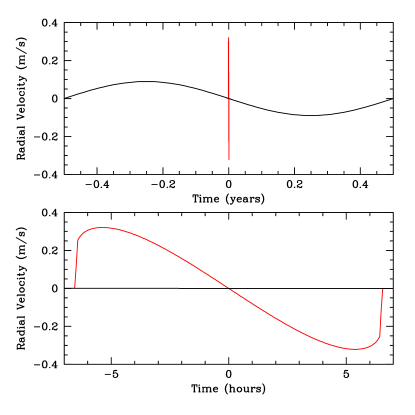
The requirements for the detection of the RM effect of a transiting habitable planet are generally less severe, both because the amplitude of the RM effect is larger than the orbital signal, as discussed in §2, and because the time scale over which stability must be maintained is much shorter. Both of these points are illustrated in Fig. 6. The $S/N$ of the RM effect is approximately

$$\left(\frac{S}{N}\right)_{R}=Q_{R}\left[\frac{1}{3}(1-4b^{2})\cos^{2}{\lambda}+b^{2}\right]^{1/2}.$$ (26)

Note that for $\lambda=0$, $(S/N)_{R}=Q_{R}\sqrt{(1-b^{2})/3}$, whereas for $\lambda=90^{\circ}$, $(S/N)_{R}=Q_{R}b$. Assuming $\sigma\sim 1~{}{\rm m\,s^{-1}}$ as above, $M=M_{\odot}$, $R=R_{\odot}$, $b=0.5$, and continuous measurements during a single transit (i.e. $N_{R}=11.23~{}{\rm hr}/1~{}{\rm hr}$), we find

$$\left(\frac{S}{N}\right)_{R}\sim 0.7\left(\frac{a}{{\rm AU}}\right)^{1/4}\left(\frac{m}{M_{\oplus}}\right)^{2/3}\left(\frac{V}{5~{}{\rm km\,s^{-1}}}\right)10^{-0.2(m_{V}-12)}\left(\frac{D}{3.6{\rm m}}\right),$$ (27)

Thus the $S/N$ with which the RM effect is measured with only $N_{R}=11$ points during transit is roughly equivalent to the $S/N$ with which the orbital Doppler shift is measured with $N_{O}=100$ points. Furthermore, detection of the RM effect only requires stability at the $\sim$$0.4~{}{\rm m\,s^{-1}}$ level for $\sim$11 hours, as opposed to a year.

A downside to RM confirmation is that it must take place on the particular nights when a transit occurs, making the effort especially vulnerable to the vagaries of the weather. And of course, since the transit only represents a small fraction of the planet’s orbit, it is possible to acquire many more data points on the orbital velocity curve than on the RM curve; it is possible to gain in the $S/N$ by a factor of $\sqrt{\pi a/R}$, where $a$ is the planet’s semimajor axis. However, in practice it will be difficult to fully realize this additional factor, because it is not possible to acquire data continuously (due to telescope availability, weather, seasonal observability, and so forth), and because the stability requirements are harder to achieve for measurements over this longer time baseline.

Nevertheless, the fact that the expected $S/N$ is substantially less than unity even for continuous observations implies that it will only be possible to verify the most favorable candidates with current setups. Assuming that we can simply scale the photon noise uncertainties obtained by HARPS to larger apertures, we find that apertures of $\sim 20-40~{}{\rm m}$ will be required to confirm [with $(S/N)_{R}=5$] the habitable transiting planets orbiting $m_{V}=12$ primaries detected by Kepler.

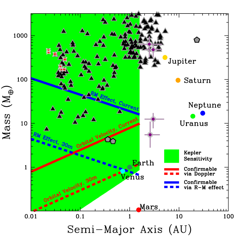
Figure 7 summarizes the prospects for the detection of planets via Kepler and the prospects for the confirmation of those planets via spectroscopic detection of either the orbital velocity or the RM effect. We show the region of parameter space in the $m-a$ plane in which Kepler can detect transiting planets orbiting stars with apparent magnitude $m_{V}=12$, assuming at least two transits are required for detection, and $(S/N)_{T}\geq 8$. By design, Kepler is (just) sensitive to Earth-mass planets in the habitable zone. We also show the region of parameter space in which planets can be confirmed (with $S/N\geq 5$) by detecting either the orbital velocity or the RM effect using current facilities, and using the expected capabilities of future 30m telescopes.

6. Summary and Discussion

The transit of an exoplanet is a rare and information-rich event that should be exploited in every possible way. In this paper we have examined one aspect of transit physics, the Rossiter-McLaughlin effect, whose origin is the rotation of the parent star. Our goal has been to assess the ability of near-term observations to exploit the information in the RM signal.

We have calculated the achievable accuracy with which one can measure the key parameter $\lambda$, with which one can assess the degree of alignment between the stellar spin axis and the planetary orbit, and have assessed the prospects for the currently known sample of transiting exoplanets. One might ask further: how accurately must $\lambda$ be known in order to enable interesting theoretical advances, such as the discrimination among different planetary migration theories? In other words, how good is good enough? This question does not seem to have been addressed in the literature on planet formation theory, and is an appealing topic for future research. As suggested in § 3, for a system with a very hot Jupiter, even a crude measurement with $\sigma_{\lambda}=30\arcdeg$ would be of interest. As a more general benchmark, one would like to achieve at least enough accuracy to tell whether a given system is similar to the Solar system, or not. To date, the only system that has been observed with enough precision for this task is HD 209458, and the result is that it is Solar-like with a small but significant misalignment of $\lambda\approx-4\arcdeg$ (Winn et al. 2005). A system could be different either by having a larger misalignment ($\lambda\lower 2.15277pt\hbox{$\;\buildrel>\over{\sim}\;$}10\arcdeg$), for which an accuracy of a few degrees or more would suffice, or by having a more perfect alignment, for which an accuracy of $\sim 0.1\arcdeg$ would be needed.

We have also explained and quantified the potentially important role of the RM effect in the confirmation of transiting planet candidates. It is a difficult task, but in many cases it will be easier than the task of detecting the orbital velocity of the parent star. The comparative advantages of RM confirmation are that the velocity amplitude is generally larger, and the acceleration is certainly larger. The full range of RM variations occur during a single transit (typically a single night or two) whereas the orbital velocity variations occur over the full orbital period (a year, for the interesting case of an Earth analog). A disadvantage of RM confirmation is that one does not learn the planetary mass; it is not a dynamical measurement, per se, but rather an alternate method of verifying that a portion of the stellar surface is periodically occulted. Furthermore, RM observations must take place during transits, whereas the spectroscopic orbital data can be obtained on any other nights. In addition, the ease or difficulty of the RM method depends on the rotation rate of the star, which will vary from system to system.

Another interesting question for future research is whether or not the RM effect could ever profitably become the basis of a planet search technique, rather than simply a follow-up technique. Ohta et al. (2005) suggested that transiting planets might announce themselves through large outliers in data bases of radial velocity measurements. The relevant efficiency factors, selection effects, and detection algorithms for such an undertaking have yet to be worked out. Even less certain are the prospects for an RM-based transit survey, in which stars are spectroscopically monitored specifically for transits. The obvious drawback is that typical high-resolution spectrographs examine only one star at a time, whereas photometric transit surveys observe thousands or even millions of stars at a time. There are plans for multiplexed Doppler spectrographs in the near future (Ge et al. 2004), but the multiplexing factor is only $\sim$50.

On the other hand, the RM effect is perhaps uniquely sensitive to small planets around hot and rapidly rotating stars. The amplitude of the RM effect depends on the stellar radius and projected rotation speed, according to Eq. (6), but these factors are not completely independent. Among main-sequence stars, both the stellar radius and the typical rotation speed increase with stellar mass (or temperature), with an especially dramatic rise near the F5 boundary. The typical rotation speed of G0 stars is $\sim$10 km s^-1, and for F0 stars it is $\sim$100 km s^-1 (see, e.g., Tassoul 2000). This is related to the strong variation in the depth of the convective zone across this same boundary. We have attempted to illustrate the net effect of these astrophysical correlations on the strength of the RM signal, in the following manner. We considered main-sequence stars ranging in spectral type from O5 to G0, and imagined that a Jupiter-sized planet makes an equatorial transit of each star. We calculated $K_{R}$ using estimates of the stellar radius from Cox et al. (2000), and estimates of typical rotation speeds from Tassoul (2000). The results are shown in Fig. 8. The maximum signal is achieved for late A stars. Of course, the achievable velocity accuracy is also a function of stellar type, as it depends on the number and width of absorption lines available for velocity determination. We have not attempted to quantify the velocity accuracy because in this regime it would certainly be advantageous to abandon the description of the RM effect as a net Doppler shift and model the distortion directly, as is done in Doppler-imaging algorithms.

Figure 8.— Rough estimate of the amplitude of the RM effect of a transiting Jovian planet as a function of the spectral type of the parent star. The effect reaches a maximum for late A stars, which is a compromise between the faster rotation rates and the larger radii of hot stars.

As with so many other areas of stellar and planetary physics, interest in the Rossiter-McLaughlin effect has been re-invigorated by the discovery of exoplanets. It has been nearly 100 years since the first observations of this effect, and yet we believe that there are still important applications waiting to be developed.

References

- Alonso et al. (2004) Alonso, R., et al. 2004, ApJ, 613, L153
- Agol et al. (2005) Agol, E., Steffen, J., Sari, R., & Clarkson, W. 2005, MNRAS, 359, 567
- Baglin (2003) Baglin, A. 2003, Advances in Space Research, 31, 345
- Bakos et al. (2004) Bakos, G., Noyes, R. W., Kovács, G., Stanek, K. Z., Sasselov, D. D., & Domsa, I. 2004, PASP, 116, 266
- Bakos et al. (2006) Bakos, G., et al. 2006, ApJ, submitted (astro-ph/0603291)
- Baraffe et al. (2003) Baraffe, I., Chabrier, G., Barman, T. S., Allard, F., & Hauschildt, P. H. 2003, A&A, 402, 701
- Barnes et al. (2005) Barnes, J. R., Cameron, A. C., Donati, J.-F., James, D. J., Marsden, S. C., & Petit, P. 2005, MNRAS, 357, L1
- Barnes & Fortney (2004) Barnes, J. W., & Fortney, J. J. 2004, ApJ, 616, 1193
- Borucki et al. (2001) Borucki, W. J., Caldwell, D., Koch, D. G., Webster, L. D., Jenkins, J. M., Ninkov, Z., & Showen, R. 2001, PASP, 113, 439
- Borucki et al. (2003) Borucki, W. J., et al. 2003, Proc. SPIE, 4854, 129
- Bouchy et al. (2004) Bouchy, F., Pont, F., Santos, N. C., Melo, C., Mayor, M., Queloz, D., & Udry, S. 2004, A&A, 421, L13
- Bouchy et al. (2005a) Bouchy, F., Pont, F., Melo, C., Santos, N. C., Mayor, M., Queloz, D., & Udry, S. 2005a, A&A, 431, 1105
- Bouchy et al. (2005b) Bouchy, F., Bazot, M., Santos, N. C., Vauclair, S., & Sosnowska, D. 2005b, A&A, 440, 609
- Bouchy et al. (2005c) Bouchy, F., et al. 2005c, A&A, 444, L15
- Brown et al. (2001) Brown, T. M., Charbonneau, D., Gilliland, R. L., Noyes, R. W., & Burrows, A. 2001, ApJ, 552, 699
- Bundy & Marcy (2000) Bundy, K. A., & Marcy, G. W. 2000, PASP, 112, 1421
- Burrows et al. (2003) Burrows, A., Sudarsky, D., & Hubbard, W. B. 2003, ApJ, 594, 545
- Butler et al. (1996) Butler, R. P., Marcy, G. W., Williams, E., McCarthy, C., Dosanjh, P., & Vogt, S. S. 1996, PASP, 108, 500
- Charbonneau et al. (2000) Charbonneau, D., Brown, T. M., Latham, D. W., & Mayor, M. 2000, ApJ, 529, L45
- Charbonneau et al. (2002) Charbonneau, D., Brown, T. M., Noyes, R. W., & Gilliland, R. L. 2002, ApJ, 568, 377
- Charbonneau et al. (2004) Charbonneau, D. 2004, in From Planets to Cosmology: Essential Science in Hubble’s Final Years (astro-ph/0410674)
- Charbonneau et al. (2005) Charbonneau, D., et al. 2005, ApJ, 626, 523
- Charbonneau et al. (2006) Charbonneau, D., et al. 2006, ApJ, 636, 445
- Charbonneau et al. (2006) Charbonneau, D., Brown, T. M., Burrows, A., & Laughlin, G. 2006, in Protostars and Planets V, in press (astro-ph/0603376 )
- Collier Cameron et al. (2002) Collier Cameron, A., Donati, J.-F., & Semel, M. 2002, MNRAS, 330, 699
- da Silva et al. (2006) da Silva, R., et al. 2006, A&A, 446, 717
- Deming et al. (2005) Deming, D., Seager, S., Richardson, L. J., & Harrington, J. 2005, Nature, 434, 740
- Deming et al. (2006) Deming, D., Harrington, J., Seager, S., & Richardson, L. J. 2006, ApJ, in press (astro-ph/0602443)
- Dunham et al. (2004) Dunham, E. W., Mandushev, G. I., Taylor, B. W., & Oetiker, B. 2004, PASP, 116, 1072
- Fischer et al. (2005) Fischer, D. A., et al. 2005, ApJ, 620, 481
- Forbes (1911) Forbes, G. 1911, MNRAS, 71, 578
- Ford et al. (2001) Ford, E. B., Havlickova, M., & Rasio, F. A. 2001, Icarus, 150, 303
- Ford & Rasio (2006) Ford, E. B., & Rasio, F. A. 2006, ApJ, 638, L45
- Fortney et al. (2006) Fortney, J. J., Saumon, D., Marley, M. S., Lodders, K., & Freedman, R. S. 2006, ApJ, 642, 495
- Gaudi (2003) Gaudi, B. S. 20003 (astro-ph/0307280)
- Gaudi (2005) Gaudi, B. S. 2005, ApJ, 628, L73
- Gaudi et al. (2005) Gaudi, B. S., Seager, S., & Mallen-Ornelas, G. 2005, ApJ, 623, 472
- Ge et al. (2004) Ge, J., Mahadevan, S., van Eyken, J. C., DeWitt, C., Friedman, J., & Ren, D. 2004, Proc. SPIE, 5492, 711
- Gimenez (2006) Gimenez, A. 2006, ApJ, in press
- Golimowski et al. (2006) Golimowski, D. A., et al. 2006, AJ, 131, 3109
- Gould (2003) Gould, A. 2003 (astro-ph/0310577)
- Gould et al. (2004) Gould, A., Gaudi, B.S., & Han, C. 2003 (astro-ph/0405217)
- Gould et al. (2006) Gould, A., Dorsher, S, Gaudi, B.S., & Udalski, A. 2006, Acta Astronomica, 56, 1
- Guillot & Showman (2002) Guillot, T., & Showman, A. P. 2002, A&A, 385, 156
- Guillot (2005) Guillot, T. 2005, Annual Review of Earth and Planetary Sciences, 33, 493
- Henry et al. (1995) Henry, G. W., Eaton, J. A., Hamer, J., & Hall, D. S. 1995, ApJS, 97, 513
- Henry et al. (2000) Henry, G. W., Marcy, G. W., Butler, R. P., & Vogt, S. S. 2000, ApJ, 529, L41
- Herbst et al. (2006) Herbst, W., Dhital, S., Francis, A., Lin, L., Tresser, N. & Williams, E. 2006, PASP, in press [astro-ph/0606164]
- Holman & Murray (2005) Holman, M. J., & Murray, N. W. 2005, Science, 307, 1288
- Holman et al. (2006) Holman, M. J. et al. 2006, in preparation
- Howard (1984) Howard, R. 1984, ARA&A, 22, 131
- Konacki et al. (2003a) Konacki, M., Torres, G., Jha, S., & Sasselov, D. D. 2003a, Nature, 421, 507
- Konacki et al. (2003b) Konacki, M., Torres, G., Sasselov, D. D., & Jha, S. 2003b, ApJ, 597, 1076
- Konacki et al. (2004) Konacki, M., et al. 2004, ApJ, 609, L37
- Konacki et al. (2005) Konacki, M., et al. 2005, ApJ, 624, 372
- Lovis et al. (2005) Lovis, C., et al. 2005, A&A, 437, 1121
- Marcy et al. (2005) Marcy, G. W., Butler, R. P., Vogt, S. S., Fischer, D. A., Henry, G. W., Laughlin, G., Wright, J. T., & Johnson, J. A. 2005, ApJ, 619, 570
- Mayor et al. (2003) Mayor, M., et al. 2003, The Messenger, 114, 20
- Mazeh et al. (2005) Mazeh, T., Zucker, S., & Pont, F. 2005, MNRAS, 356, 955
- McCullough et al. (2005) McCullough, P. R., Stys, J. E., Valenti, J. A., Fleming, S. W., Janes, K. A., & Heasley, J. N. 2005, PASP, 117, 783
- McCullough et al. (2006) McCullough, P. R., et al. 2006, ApJ, accepted (astro-ph/0605414)
- McLaughlin (1924) McLaughlin, D. B. 1924, ApJ, 60, 22
- Moutou et al. (2004) Moutou, C., Pont, F., Bouchy, F., & Mayor, M. 2004, A&A, 424, L31
- Ohta et al. (2005) Ohta, Y., Taruya, A., & Suto, Y. 2005, ApJ, 622, 1118
- Pepe et al. (2002) Pepe, F., et al. 2002, The Messenger, 110, 9
- Pepper et al. (2004) Pepper, J., Gould, A., & Depoy, D. L. 2004, AIP Conf. Proc. 713: The Search for Other Worlds, 713, 185
- Pont et al. (2004) Pont, F., Bouchy, F., Queloz, D., Santos, N., Melo, C., Mayor, M., & Udry, S. 2004, A&A, 426, L15
- Pont et al. (2005) Pont, F., Bouchy, F., Melo, C., Santos, N. C., Mayor, M., Queloz, D., & Udry, S. 2005, A&A, 438, 1123
- Rasio & Ford (1996) Rasio, F. A., & Ford, E. B. 1996, Science, 274, 954
- Rauer et al. (2004) Rauer, H., Erikson, A., Voss, H., Titz, R., Hatzes, A. P., Eislöffel, J., & Guenther, E. 2004, Astronomische Nachrichten, 325, 574
- Remijan & Hollis (2006) Remijan, A. J., & Hollis, J. M. 2006, ApJ, 640, 842
- Rice (2002) Rice, J. B. 2002, Astronomische Nachrichten, 323, 220
- Queloz et al. (2000) Queloz, D., Eggenberger, A., Mayor, M., Perrier, C., Beuzit, J. L., Naef, D., Sivan, J. P., & Udry, S. 2000, A&A, 359, L13
- Reiners (2006) Reiners, A. 2006, A&A, 446, 267
- Rossiter (1924) Rossiter, R. A. 1924, ApJ, 60, 15
- Rucinski et al. (2004) Rucinski, S. M., et al. 2004, PASP, 116, 1093
- Seager & Hui (2002) Seager, S., & Hui, L. 2002, ApJ, 574, 1004
- Sato et al. (2005) Sato, B., et al. 2005, ApJ, 633, 465
- Schlesinger (1911) Schlesinger, F. 1911, MNRAS, 71, 719
- Snellen (2004) Snellen, I. A. G. 2004, MNRAS, 353, L1
- Sozzetti et al. (2004) Sozzetti, A., et al. 2004, ApJ, 616, L167
- Steffen & Agol (2005) Steffen, J. H., & Agol, E. 2005, MNRAS, 364, L96
- Street et al. (2004) Street, R. A., et al. 2004, Astronomische Nachrichten, 325, 565
- Udalski et al. (2002a) Udalski, A., et al. 2002a, Acta Astronomica, 52, 1
- Udalski et al. (2002b) Udalski, A., Zebrun, K., Szymanski, M., Kubiak, M., Soszynski, I., Szewczyk, O., Wyrzykowski, L., & Pietrzynski, G. 2002a, Acta Astronomica, 52, 115
- Udalski et al. (2002c) Udalski, A., Szewczyk, O., Zebrun, K., Pietrzynski, G., Szymanski, M., Kubiak, M., Soszynski, I., & Wyrzykowski, L. 2002c, Acta Astronomica, 52, 317
- Udalski et al. (2003) Udalski, A., Pietrzynski, G., Szymanski, M., Kubiak, M., Zebrun, K., Soszynski, I., Szewczyk, O., & Wyrzykowski, L. 2003, Acta Astronomica, 53, 133
- Vidal-Madjar et al. (2003) Vidal-Madjar, A., Lecavelier des Etangs, A., Désert, J.-M., Ballester, G. E., Ferlet, R., Hébrard, G., & Mayor, M. 2003, Nature, 422, 143
- Welsh et al. (2004) Welsh, W. F., Orosz, J. A., & Wittenmyer, R. A. 2004, American Astronomical Society Meeting Abstracts, 205, #135.16
- Winn & Holman (2005) Winn, J. N., & Holman, M. J. 2005, ApJ, 628, L159
- Winn et al. (2005) Winn, J. N., et al. 2005, ApJ, 631, 1215
- Wittenmyer et al. (2005) Wittenmyer, R. A., et al. 2005, ApJ, 632, 1157
- Wolf et al. (2006) Wolf, A.S. et al. 2006, ApJ, in press
- Wu & Murray (2003) Wu, Y., & Murray, N. 2003, ApJ, 589, 605