Dynamical Evolution of Globular Clusters in Hierarchical Cosmology

Abstract

We test the hypothesis that metal-poor globular clusters form within disk galaxies at redshifts $z>3$. Numerical simulations demonstrate that giant gas clouds, which are cold and dense enough to produce massive star clusters, assemble naturally in hierarchical models of galaxy formation at high redshift. Do model clusters evolve into observed globular clusters or are they disrupted before present as a result of the dynamical evolution? To address this question, we calculate the orbits of model clusters in the time-variable gravitational potential of a Milky Way-sized galaxy, using the outputs of a cosmological $N$-body simulation. We find that at present the orbits are isotropic in the inner 50 kpc of the Galaxy and preferentially radial at larger distances. All clusters located outside 10 kpc from the center formed in satellite galaxies, some of which are now tidally disrupted and some of which survive as dwarf galaxies. The spatial distribution of model clusters is spheroidal and the fit to the density profile has a power-law slope $\gamma\approx 2.7$, somewhat shallower than but consistent with observations of metal-poor clusters in the Galaxy. The combination of two-body relaxation, tidal shocks, and stellar evolution drives the evolution of the cluster mass function from an initial power law to a peaked distribution, in agreement with observations. However, not all initial conditions and not all evolution scenarios are consistent with the observed mass function of the Galactic globular clusters. The successful models require the average cluster density, $M/R_{h}^{3}$, to be constant initially for clusters of all mass and to remain constant with time. Synchronous formation of all clusters at a single epoch ($z=4$) and continuous formation over a span of 1.6 Gyr (between $z=9$ and $z=3$) are both consistent with the data. For both formation scenarios, we provide online catalogs of the main physical properties of model clusters.

1. Introduction

Observations in the past decade with the Hubble Space Telescope and major ground-based telescopes have revolutionized the field of star cluster research. The classical division into old, massive globular clusters and young, diffuse open clusters has been challenged by the discoveries of young massive star clusters in nearby merging, interacting, and even normal star forming galaxies (e.g., Holtzman et al., 1992; Whitmore et al., 1993; Whitmore & Schweizer, 1995; O’Connell et al., 1995; Zepf et al., 1999; Larsen, 2002). These young clusters have the range of masses and sizes similar to Galactic globulars and are believed to evolve eventually into globular clusters (e.g., Ho & Filippenko, 1996; Mengel et al., 2002; de Grijs et al., 2004). However, the mass functions of old and young clusters are very different. While the mass distribution of globular clusters has a well-defined peak at $\approx 2\times 10^{5}\,\mathrm{M}_{\odot}$, the mass function of young clusters is consistent with a single power law between $10^{4}$ and $10^{7}\,\mathrm{M}_{\odot}$ (Zhang & Fall, 1999; de Grijs et al., 2003; Anders et al., 2004). Did old globular clusters form by a similar physical process to the young clusters but gradually evolve into the observed distribution?

This question is vital to understanding early galaxy formation and is still a matter of debate (Fall & Zhang, 2001; Vesperini et al., 2003). Globular clusters contain relic information about star formation processes in galaxies at high redshift and have been often used to constrain cosmological theory. Uncovering the formation of primeval galaxies is a major driving force behind the development of future major ground and space observatories. In contrast to the formidable difficulties of detecting the birthplaces of globular clusters at high redshift, local and interacting galaxies (M33, M51, M82, the Antennae) offer plenty of detail of the formation of young star clusters in giant molecular clouds (Wilson et al., 2003; Engargiola et al., 2003; Keto et al., 2005). Using ultrahigh-resolution cosmological simulation, Kravtsov & Gnedin (2005) identified similar molecular clouds within their simulated high-redshift galaxies and proposed that they harbor massive star clusters. In this paper, we investigate whether the dynamically-evolved distribution of these model clusters can be reconciled with the current properties of globular clusters.

Kravtsov & Gnedin (2005) find that giant clouds assemble during gas-rich mergers of progenitor galaxies, when the available gas forms a thin, cold, self-gravitating disk. The disk develops strong spiral arms, which further fragment into separate molecular clouds located along the arms as beads on a string (see their Fig. 1). As a result, massive clusters form in relatively massive galaxies, with the total mass $M_{\rm halo}>10^{9}\ \mathrm{M}_{\odot}$, beginning at redshift $z\approx 10$. The mass and density of the molecular clouds increase with cosmic time, but the rate of galaxy mergers declines steadily. Therefore, the cluster formation efficiency peaks at a certain extended epoch, around $z\approx 4$, when the Universe is only 1.5 Gyr old. The mass function of model clusters is consistent with a power law

$$dN/dM=N_{0}\,M^{-\alpha},$$ (1)

where $\alpha=2.0\pm 0.1$, similar to the observations of nearby young star clusters. According to the prescription for metal enrichment by supernovae in the Kravtsov & Gnedin (2005) simulation, model clusters have iron abundances $[Fe/H]\leq-1$ at $z>3$. They correspond to the metal-poor (dominant) sub-population of the Galactic globular clusters, which we will use for the comparison.

We adopt this model to set up the initial positions, velocities, and masses for our globular clusters. We then calculate cluster orbits using the results of a separate collisionless $N$-body simulation described in § 2. This is necessary because the original gasdynamics simulation was stopped at $z\approx 3$, due to limited computational resources. By using the $N$-body simulation of a similar galactic system, but complete to $z=0$, we are able to follow the full dynamical evolution of globular clusters until the present epoch. We use the evolving properties of all progenitor halos, from the outputs with a time resolution of $\sim 10^{8}$ yr, to derive the gravitational potential in the whole computational volume at all epochs. We convert a fraction of the dark matter mass into the analytical flattened disks, in order to model the effect of baryon cooling and star formation on the galactic potential. We calculate the orbits of globular clusters in this potential from the time when their host galaxies accrete onto the main (most massive) galaxy. Using these orbits, we calculate the dynamical evolution of model clusters, including the effects of stellar mass loss, two-body relaxation, tidal truncation, and tidal shocks. Since the efficiency of each of these processes depends on both cluster mass, $M$, and half-mass radius, $R_{h}$, we consider several evolutionary dependencies $R_{h}(M)$. We also consider two possible formation scenarios, one with all clusters forming in a short interval of time around redshift $z=4$, and the other with a continuous formation of clusters between $z=9$ and $z=3$.

Note that we study only the collisionless evolution of star clusters, using the analytical formalism developed in previous studies and described in § 3. We do not include the recently suggested “infant mortality” effect, which may dissolve a large number of unbound clusters within $\sim 100$ Myr of their formation independent of cluster mass (e.g., Fall et al., 2005; Mengel et al., 2005). Such universal reduction in numbers is therefore absorbed in our normalization of the initial GCMF. The models calculated in this paper apply only to the initially bound clusters.

2. Orbits of Globular Clusters in a Hierarchically-Forming Galaxy

2.1. Cosmological Simulation

We set the initial conditions and calculate the orbits of model clusters using a cosmological $N$-body simulation performed with the Adaptive Refinement Tree code (ART, Kravtsov et al., 1997; Kravtsov, 1999). This simulation follows the hierarchical formation of a Milky Way-sized halo in a comoving box of $25h^{-1}$ Mpc in the concordance $\Lambda$CDM cosmology: $\Omega_{\rm m}=0.3$, $\Omega_{\Lambda}=0.7$, $\sigma_{8}=0.9$, $H_{0}=70$ km s^-1 Mpc^-1. The simulation begins with a uniform $256^{3}$ grid covering the entire computational volume. High mass resolution is achieved around collapsing structures by recursive refinement of this regions using an adaptive refinement algorithm. The grid cells are refined if the particle mass contained within them exceeds a certain threshold value. Thus, this adaptive grid follows the collapsing galaxy in a quasi-lagrangian fashion. With maximum 10 levels of refinement, the peak formal spatial resolution is 0.15 comoving kpc. This simulation is described in more detail in Kravtsov et al. (2004).

Halos and subhalos are identified using a variant of the Bound Density Maxima algorithm (Klypin et al., 1999). The halo finder algorithm produces halo catalogs, which contain positions, velocities, and main properties of the dark matter halos between $z=9$ and $z=0$ at 96 output times, with a typical separation between outputs $\approx 10^{8}$ yr. The main properties of the halos in the catalogs are: the virial radius ($r_{\rm vir}$), truncation radius ($r_{\rm t}$), halo radius ($r_{\rm halo}=\min[r_{\rm t},r_{\rm vir}]$), halo mass ($M_{\rm halo}$), maximum circular velocity ($V_{\rm max}$) and the corresponding radius at which the maximum velocity is reached ($r_{\rm max}$). The virial radius (and corresponding virial mass) is defined as the radius within which the density is 180 times the mean density of the Universe. The truncation radius is the radius at which the logarithmic slope of the density profile becomes larger than -0.5, since we do not expect the density profile of the halos to be flatter than this slope. If the center of a halo does not lie within the boundary of a larger system, its radius $r_{\rm halo}$ is defined equal to the virial radius. On the other hand, if the halo is within another halo (and is therefore a subhalo), its radius is the truncation radius. The halo mass follows the same definition: $M_{\rm halo}=\min[M(r_{\rm t}),M(r_{\rm vir})]$.

In this paper, we consider the evolution of an isolated halo G₁, which we call the main halo. This halo contains over $10^{6}$ particles within its virial radius at $z=0$. The virial mass at $z=0$ in our definition is $M_{\rm vir}=2.37\times 10^{12}\,\mathrm{M}_{\odot}$, the virial radius $r_{\rm vir}=426$ kpc and the halo concentration $c=13$. For the commonly used overdensity of 340, the virial mass and radius are $M_{340}=2.07\times 10^{12}\,\mathrm{M}_{\odot}$ and $r_{340}=330$ kpc, respectively. The main halo has experienced the last major merger at $z\approx 2$ and therefore could subsequently host a large spiral galaxy.

The main advantage of the catalogs of Kravtsov et al. (2004) is that they trace the progenitors of halos at previous epochs and therefore allow us to reconstruct the full dynamical evolution of the model galaxies. This information is necessary to follow the evolution of globular clusters within their host galaxies, before being accreted onto the main halo.

2.2. Galactic Potential

We construct realistic time-dependent galactic potentials using the halo catalogs and supplementing each massive dark matter halo with a baryonic disk. The distribution of dark matter in a cosmological simulation can be approximately described as a combination of isolated halos and satellites within them, and therefore the gravitational potential can be approximated by a sum of the potentials of the main halo and all subhalos (Kravtsov et al., 2004). For each galaxy (isolated and satellite) we assign a fraction of the mass, $M_{\rm disk}=f_{\rm d}\,M_{\rm halo}$, to the baryonic disk and the remaining mass, $(1-f_{\rm d})M_{\rm halo}$, to the dark halo. In this crude approximation, the fraction $f_{\rm d}$ accounts for the potential of stars and cold gas in the galaxy and absorbs all the complex details of star formation. We do not explicitly consider the galactic bulge because most cluster orbits do not come too close to the bulge, and its potential can be described by the inner part of the disk. The bulge mass is therefore absorbed in our definition of the disk mass. The total potential, as a function of space and time, is the sum of the halo and disk contributions of all the galaxies:

$$\Phi(\mbox{\boldmath$r$},t)=\sum_{i}\Phi_{\rm halo}^{i}(\mbox{\boldmath$r$}-\mbox{\boldmath$r$}_{i})+\Phi_{\rm disk}^{i}(\mbox{\boldmath$r$}-\mbox{\boldmath$r$}_{i}),$$ (2)

where $\mbox{\boldmath$r$}_{i}$ is the position of the center of mass of halo $i$ at time $t$.

We assume that the dark matter potential of each galaxy is given by a spherical NFW (Navarro et al., 1997) profile:

$$\Phi_{\rm halo}(r)=-{GM_{\rm halo}(1-f_{d})\over r}{\ln{(1+r/r_{\rm s})}\over\ln{(1+c)}-c/(1+c)}$$ (3)

where $c=r_{\rm halo}/r_{\rm s}$ is the halo concentration, and $r_{s}$ is the scale radius approximated as $r_{s}\approx r_{\rm max}/2.16$. We use this latter relation because the profiles of some of the smaller subhalos are not well resolved in the simulation and the radius $r_{\rm max}$ is better constrained than $r_{s}$. The axisymmetric disk potential is modeled with a Miyamoto & Nagai (1975) profile, in cylindrical coordinates ($R,Z$):

$$\Phi_{\rm disk}(R,Z)=-\frac{GM_{\rm disk}}{\sqrt{R^{2}+(a_{\rm d}+\sqrt{Z^{2}+b_{\rm d}^{2}})^{2}}}$$ (4)

where $M_{\rm disk}(t)$, $a_{\rm d}(t)$ and $b_{\rm d}(t)$ are the mass, radial scale length, and vertical scale height of the disk, respectively, which vary with time.

The masses and sizes of the halos are linearly interpolated between the output epochs in the halo catalog. For the parameters of the disk, we apply the following simple model. The disk mass increases linearly in time from the initial epoch $z=9$ to the redshift of accretion $z_{\rm acc}$. This is defined as the epoch when the halo is accreted onto the main halo, i.e., when its center of mass is within the virial radius of the main halo. We stop the growth of the disk when it is accreted and keep its mass fixed at later times, regardless of the evolution of its host halo. For the main halo and other isolated halos, $z_{\rm acc}=0$ by definition. Thus the initial disk mass is $f_{\rm d}\,M_{\rm halo}(z=9)$ and the final mass is $f_{\rm d}\,M_{\rm halo}(z=z_{\rm acc})$. We set $f_{\rm d}=0.05$, consistent with the value inferred for the Milky Way (Klypin et al., 2002).

We use a similar recipe to obtain the scale length $a_{\rm d}(t)$ as a function of time, by requiring $a_{\rm d}=0.02\,r_{\rm halo}$. It is interesting to note that $a_{\rm d}$ for the Miyamoto & Nagai (1975) disk is equal within $3\%$ to the exponential scale length, $r_{\rm d}$, defined as the radius at which the surface density decreases by a factor $\Sigma(0)/\Sigma(r_{\rm d})\equiv e$. The ratio of the vertical scale height to the radial scale length is set constant at all times, $b_{\rm d}/a_{\rm d}=0.2$, consistent with observed galaxy disks (e.g., Binney & Tremaine, 1987). In our model, the disk of the main galaxy has the mass $M_{\rm disk}=1.2\times 10^{11}\,\mathrm{M}_{\odot}$ and scale length $a_{\rm d}=8.5$ kpc at $z=0$. Both of these parameters are probably a factor of 2 larger than in the Milky Way, as is the total halo mass.

We use proper (not comoving) coordinates and a reference frame where the main halo is at the origin of the coordinate system at all times. With the potential given by equation (2), the acceleration of a test particle at ($r$,$t$) is calculated analytically:

$$\mbox{\boldmath$a$}=-\mbox{\boldmath$\nabla$}_{r}\Phi+\Omega_{\Lambda}\,H_{0}^{2}\,\mbox{\boldmath$r$}.$$ (5)

The second term in this equation is a constant acceleration per unit length due to the dark energy, parametrized by the cosmological constant (Lahav et al., 1991). It affects only clusters outside 200 kpc from the center. We use cubic spline interpolation between the outputs of the halo catalogs to obtain the positions of halos at intermediate times. The third order spline assures that the halo velocities are smooth functions and the accelerations are continuously defined at each catalog output. However, this non-linear interpolation of subhalo motions creates an additional acceleration of the globular clusters within them, which needs to be included in equation (5).

2.3. Initial Conditions for Globular Clusters

In the model of Kravtsov & Gnedin (2005), globular clusters form in dense cores of giant molecular clouds within the disks of high-redshift galaxies. We adopt this model to set the initial masses, positions, and velocities of the clusters in each massive halo, $M_{\rm halo}>10^{9}\,\mathrm{M}_{\odot}$. We use the initial globular cluster mass function (GCMF) given by equation (1), with the slope $\alpha=2$ and the normalization such that the total mass in globular clusters in that halo, $M_{GC}$, scales with the host halo mass as found in the simulation of Kravtsov & Gnedin (2005):

$$M_{GC}=3.2\times 10^{6}\,\mathrm{M}_{\odot}\left(\frac{M_{\rm halo}}{10^{11}\,\mathrm{M}_{\odot}}\right)^{1.13}\times f.$$ (6)

The additional scaling factor, $f\geq 1$, is needed for those models where we assume that all clusters form at a single epoch rather than over an extended period. We choose this normalization factor such that the number of surviving clusters at $z=0$ is approximately equal to the number of observed metal poor clusters in the Galaxy. For the best model Sb-ii (see below) we have $f=12$; the continuous formation model Cb-ii does not require a change in the normalization: $f=1$. We adopt the lower limit for the initial GCMF as $M_{\rm min}=10^{5}\,\mathrm{M}_{\odot}$ and the upper limit, $M_{\rm max}$, given by the fit of Kravtsov & Gnedin (2005) scaled by the same factor $f$. The choice of the lower mass limit is motivated by our disruption calculations, which show that no cluster of lower mass is expected to survive the dynamical evolution over 10 Gyr (see § 4). The actual number of clusters in each host galaxy is given by the discretization of the mass function.

After being accreted into the main halo, some host halos are tidally disrupted. There are a total of 77 halos that host globular clusters within the virial radius of the main galaxy, of which 37 are disrupted and 40 survive until $z=0$. 80% of all host halos are accreted in the redshift range $z_{\rm acc}\approx 0.2-1.9$. The surviving halos are accreted systematically later than the disrupted halos. The median redshift of accretion for all halos is 1.2, while for the surviving subhalos it is 0.64.

We assume that the spatial number density of globular clusters follows the distribution of baryon mass in their host galaxy disk: $dN(R)\propto\Sigma_{\rm d}(R)\,R\,dR$, where $\Sigma_{\rm d}(R)$ is the disk surface density. We use this equation to obtain the initial radial positions of the clusters, $R$. We assign their azimuthal angles and vertical positions randomly from the uniform distributions in the intervals [0, $2\pi$] and [$-b_{\rm d}$, $+b_{\rm d}$], respectively. There is no correlation between the initial cluster masses and positions. The clusters are set on circular orbits parallel to the plane of the disk, with the initial velocities equal $V_{c}=\sqrt{GM(R)/R}$, where $M(R)$ is the total halo plus disk mass within radius $R$. The initial velocities of both halos and globular clusters include also the Hubble expansion velocity.

We consider two sets of cluster formation models:

1. Single epoch of formation (S). The clusters form at $z_{f}=4$ in galaxies with $M_{\rm halo}>10^{9}\,\mathrm{M}_{\odot}$. The masses and positions of clusters are generated using the masses and sizes of the halos at $z_{f}$, but the velocities are obtained using the halo properties at the epoch of accretion. In the case of the main halo, orbit integration starts at $z=4$.

2. Continuous formation (C). Clusters form continuously in the redshift range $9\geq z_{f}\geq 3$, at each of the original gasdynamics simulation outputs. The average time interval between the simulation outputs is $7\times 10^{7}$ yr. The span of cosmic time between $z=9$ and $z=3$ is approximately 1.6 Gyr, which is consistent the observed spread of ages of the metal-poor clusters in the Galaxy. As in model (S), the masses and positions of clusters are obtained using the halo properties at $z_{f}$ but the velocities are calculated only at $z_{\rm acc}$.

For each of these formation models, we consider several variations of the initial relation between the cluster half-mass radius and its mass and of the evolution of this relation with time. For the initial $R_{h}-M$ relation at the time of formation, we consider two models:

1. $R_{h}(0)={\rm constant}$. We use the median value for the Galactic globular clusters, calculated using the online catalog of Harris (1996): $R_{h}=2.4$ pc.

2. $R_{h}(0)\propto M(0)^{1/3}$. We use the constant average half-mass density, $\rho_{h}(0)=4\times 10^{3}\,\mathrm{M}_{\odot}\,{\rm pc}^{-3}$, from the model of Kravtsov & Gnedin (2005) and set $R_{h}=(3M/4\pi\rho_{h})^{1/3}$. The half-mass density does not depend on the position of the cluster in its host galaxy, and therefore, by construction does not reflect the local tidal field. We make this assumption for consistency with the formation model that we are testing.

For the time dependence of the $R_{h}-M$ relation, we consider three variations:

1. $R_{h}(t)={\rm constant}$,

2. $R_{h}(t)\propto M(t)^{1/3}$, i.e. $\rho_{h}(t)={\rm constant}$,

3. $R_{h}(t)\propto M(t)$.

We construct 12 different model realizations by combining the single or continuous formation of clusters (S, C) with the initial (a, b) and evolutionary (i, ii, iii) size-mass relations. In our notation, Sa-i is the model with a single redshift of formation and constant half-mass radius throughout the evolution; Cb-i has continuous formation in the redshift range $9\geq z\geq 3$, initially constant half-mass density, and constant half-mass radius thereafter, etc. These models are summarized in Table 1.

For clusters that originate in galaxies that will have become satellites of the main halo, we integrate the orbits beginning from the epoch of accretion, $z_{\rm acc}$, rather than the epoch of formation, $z_{f}$. The motivation for doing so is to avoid unnecessary computation of the orbits of clusters inside their host galaxies at $z_{f}>z>z_{\rm acc}$. Before the host galaxies are accreted into the main halo, we expect their globular clusters to remain on gravitationally-bound equilibrium orbits. For small hosts, the time step required to follow these orbits is small, which leads to two problems. One is the large number of computations, the other is gradual accumulation of integration errors. The situation changes when the host galaxy becomes a satellite – globular clusters may experience significant tidal perturbations from the main halo and may even escape their original host. Therefore, we assume that the clusters remain bound to their hosts at $z>z_{\rm acc}$ and calculate their orbits only from $z=z_{\rm acc}$ until the present. We keep the cluster positions $R$ and $Z$ assigned at $z_{f}$ (equivalent to assuming initially circular orbits) but recalculate the initial cluster velocities using the host mass at $z_{\rm acc}$.

For clusters in all models, we calculate the mass loss via two-body relaxation and stellar evolution beginning at their assumed epoch of formation, $z_{f}$. We include tidal shocks only when we begin orbit integration at $z_{\rm acc}$, because the mass loss rate due to tidal shocks is very sensitive to the cluster orbits, as described in § 3.

Figure 1.— Three types of globular clusters orbits. Left panels show the proper (not comoving) distance to the center of the main halo as a function of cosmic time, right panels show orbits in the plane of the main disk. Top: cluster formed in the main halo, on an initially circular orbit but was later scattered by accreted satellites. Middle: cluster formed in a satellite halo, which survived as a distinct galaxy (halo is shown by a dashed line). Bottom: cluster formed in a satellite that was tidally disrupted at $t\simeq 4\ {\rm Gyr}$.

2.4. Orbits of Host Halos and Globular Clusters

The orbits of clusters in a time-dependent potential presented in § 2.2 are integrated using a second-order leapfrog scheme with a fixed time step. We have chosen this symplectic integration scheme because it conserves energy to a precision of $\sim 10^{-10}$ in a static spherical potential. A typical time step is $10^{4}$ yr, which requires $\sim 10^{3}$ integration steps per cluster orbit within a satellite host and $\sim 10^{4-5}$ steps per orbit within the main halo.

Using only the outputs of an $N$-body simulation, we cannot reproduce exactly the orbits that test objects would have had in that simulation. First, finite integration errors accumulate along the orbits and diverge exponentially in time, such that two objects initially close to each other may have quite different final positions. Second, we calculate the gravitational potential by approximating the complex distribution of dark matter as a sum of spherical halos. This approximation is not entirely unreasonable and reproduces the tidal field fairly accurately (see Kravtsov et al., 2004), but of course it is not exact. We would like to test the orbit integration scheme on objects for which we know their final positions in the simulation. One class of such objects are the satellite halos that host globular clusters.

We calculate the orbits of the host halos from $z_{\rm acc}$ to the present and compare their predicted final radial distribution with the actual distribution in the $N$-body halo catalogs. In addition to the gravitational potential given by equation (2), we include the effect of dynamical friction, a drag force exerted by the main halo on the orbiting satellites, using Chandrasekhar’s formula (Chandrasekhar, 1943):

$$\mbox{\boldmath$a$}_{\rm df}=-4\pi G^{2}M_{\rm halo}\,\rho\,\ln{\Lambda}\frac{\mbox{\boldmath$v$}}{v^{3}}\left[{\rm erf}(X)-\frac{2X}{\sqrt{\pi}}e^{-X^{2}}\right],$$ (7)

where $M_{\rm halo}$ is the mass of the satellite halo, $\rho(r)$ is the local density of the main halo, $v$ is the velocity of the satellite relative to the main halo, and $X\equiv v/[2\sigma(r)]$, where $\sigma(r)$ is the one-dimensional velocity dispersion of particles in the main halo, which was calculated assuming an isotropic dispersion tensor using the approximate formula of Zentner & Bullock (2003). Assuming a constant value for the Coulomb logarithm, we find that with $\ln{\Lambda}=5$ the calculated radial distribution of satellite halos is similar to that in the halo catalogs. We somewhat overpredict the number of halos at $r<50$ kpc and underpredict this number at larger distances, with the maximum deviation of $\sim 50\%$ at 150 kpc. At even larger distances the discrepancy decreases and we match the number of halos from the catalogs again at 250 kpc. We find that dynamical friction noticeably affects the orbits of satellite halos, in an apparent disagreement with the conclusion of Peñarrubia & Benson (2005). The KS test probability that our calculated halo positions are drawn from the same distribution as the $N$-body positions is 23% with dynamical friction but only 2% without it.

Even though we do not reproduce the positions of the subhalos exactly, we find that the calculated orbits are statistically consistent with those in the simulation in the region of interest ($r<200$ kpc). This test therefore suggests that the motions of objects in a hierarchically-forming galaxy can be reasonably accurately calculated by approximating the total gravitational potential as the sum of spherical halos. We now apply this method to calculate the orbits of globular clusters.

Within the disks of progenitor galaxies, all clusters in our model begin on nearly circular orbits. Present globular clusters in the Galaxy could either have formed in the main disk, have come from the now-disrupted progenitor galaxies, or have remained attached to a satellite galaxy. Figure 1 shows the three corresponding types of cluster orbits. Even the clusters formed within the inner 10 kpc of the main Galactic disk do not stay on circular orbits. They are scattered to eccentric orbits by accreted satellites, while the growth of the disk increases the average orbital radius. Triaxiality of the dark halo (not included in present calculations) would also scatter the cluster orbits. The clusters left over from the disrupted progenitor galaxies typically lie at larger distances, between 20 and 60 kpc, and belong to the inner halo class. Their orbits are inclined with respect to the Galactic disk and are fairly isotropic. The clusters still associated with the surviving satellite galaxies are located in the outer halo, beyond 100 kpc from the Galactic center. Note that these clusters may still be scattered away from their hosts during close encounters with other satellites and consequently appear isolated.

Figure 2.— Spatial distribution of surviving clusters in the Galactic frame for model Sb-ii. Dotted circles are at projected distances of 20, 50 and 150 kpc.

Figure 3.— Number density profiles of surviving globular clusters (filled circles) in models Sb-ii (left) and Cb-ii (right) can be fit by the same power law, $n(r)\propto r^{-2.7}$. Vertical error bars are from Poisson statistics alone. The distribution of model clusters is somewhat steeper than that of surviving satellite halos (open circles), but it is similar to the distribution of smooth dark matter (dotted line, arbitrary normalization). It is also consistent with the observed distribution of metal-poor globular clusters in the Galaxy (solid line), plotted using the data from the catalog of Harris (1996).

Figure 4.— Mean eccentricity (left) and mean pericenter (right) distributions of the surviving globular clusters in models Sb-ii (top) and Cb-ii (bottom).

2.5. Spatial distribution

Hierarchical mergers of progenitor galaxies ensure that the present spatial distribution of the globular cluster system is roughly spheroidal. Figure 2 shows the positions of the surviving globular clusters in the Galactic frame, for the best-fit model Sb-ii described in § 4. Most clusters are now within 50 kpc from the center, but some are located as far as 200 kpc. The median distance is 90 kpc, which is significantly larger than the median distance of the metal-poor Galactic clusters (7 kpc). Our simulated galaxy is perhaps twice as extended as the Milky Way, but this alone is not enough to explain the discrepancy. It could be that some metal-poor clusters have formed later within the main disk, which is not included in our current model.

Figure 3 shows that the azimuthally-averaged space density of globular clusters is consistent with a power law, $n(r)\propto r^{-\gamma}$. The best models have logarithmic slopes $\gamma=2.65$ (Sb-ii) and $\gamma=2.72$ (Cb-ii). The slopes for all other models are given in Table 1. Since all of the distant clusters originate in progenitor galaxies and share similar orbits with their hosts (disrupted and survived), the distribution of the clusters is similar to the overall distribution of dark matter given by the NFW profile. The cluster profile is steeper than that of the surviving satellite halos ($\gamma\approx 2.2$), because the surviving satellites are preferentially found in the outer regions of the main halo. A higher fraction of the inner satellites is disrupted, but the globular clusters that they hosted are dense enough to survive the tidal field of the inner galaxy.

The density profile of model clusters is also similar to the observed distribution of the metal-poor ($\mbox{[Fe/H]}<-0.8$) globular clusters in the Galaxy, calculated using the online catalog of Harris (1996): $\gamma=3.15\pm 0.09$. Such comparison is appropriate, for our model of cluster formation at high redshift currently includes only low metallicity clusters ($\mbox{[Fe/H]}\leq-1$). Thus the formation of globular clusters in progenitor galaxies with subsequent merging is consistent with the observed spatial distribution of the Galactic metal-poor globulars.

We have also tested the effect of dynamical friction on the spatial distribution of clusters in our best models. We included this effect on the orbits only within the main halo, but not in the original host galaxies. We again use Chandrasekahr’s approximation for the drag force (eq. [7]), with the appropriate coulomb logarithm, $\ln{\Lambda_{\rm cl}}=12$, and replace the mass of the subhalos by the initial mass of the clusters. By using the initial cluster mass, not reduced by subsequent dynamical evolution, we consider the maximum effect that dynamical friction can have on cluster orbits. Unlike the case of the halo orbits, we find that dynamical friction does not noticeably change the cluster distribution. The density profile can again be fit by a power law with the slope that differs from the case without dynamical friction by only $\Delta\gamma=0.02$. This difference is well within the errors of the power-law fit procedure and is therefore not significant. We note that the distributions of subhalos with and without dynamical friction are also consistent within the errors, with $\Delta\gamma=0.06$.

Figure 5.— Anisotropy parameter $\beta$ as a function of radius for models Sb-ii (left) and Cb-ii (right). The vertical error bars represent the error in the mean for each radial bin, while horizontal bars show the range of the bin. Horizontal dashed lines illustrate an isotropic ($\beta=0$) and a purely radial ($\beta=1$) orbital distributions.

Several studies in the literature looked at the projected spatial distribution of globular clusters in nearby, mainly early-type galaxies. Kissler-Patig (1997) find that the surface density profiles of globular cluster systems in 15 elliptical galaxies are consistent with a power law $\sigma(R)\propto R^{-\Gamma}$, where $1.0<\Gamma<2.2$. More recent studies find similar results for elliptical galaxies: $\Gamma=1.2-1.9$ (Rhode & Zepf, 2004), $\Gamma=0.8-2.6$ (Puzia et al., 2004), $\Gamma\approx 2.0$ (Harris et al., 2004), $\Gamma\approx 1.4$ (Dirsch et al., 2005), $\Gamma=1.2-1.6$ (Forbes et al., 2006), and for a spiral galaxy NGC 7814, which has $\Gamma\approx 1.0$ (Rhode & Zepf, 2003). More luminous galaxies have shallower globular cluster profiles, in agreement with an earlier study by Harris (1986). In the inner regions, many GC system profiles have constant-density cores. In addition, in all studied cases the metal-poor globular cluster population is more spatially extended (has lower $\Gamma$) than the metal-rich population.

To make a prediction for the surface density profile of our model clusters, we project the cluster positions along random lines-of-sight and fit a power-law to the resulting distribution. After averaging over 6000 random projections, we find for the two best models: $\Gamma=1.76\pm 0.11$ (Sb-ii) and $\Gamma=1.81\pm 0.12$ (Cb-ii). These power-law slopes are consistent with the above-mentioned wide range of slopes of the globular clusters systems in elliptical and some spiral galaxies. These slopes $\Gamma$ are also consistent with the expectation for a spherical distribution of model clusters, where $\Gamma=\gamma-1$ and $\gamma=2.7$.

Forte et al. (2005) emphasize the similarity of the spatial distribution of blue globular clusters in giant elliptical NGC 1399 with that inferred for dark matter, and Cote et al. (1998) made a similar case for M87. As Figure 3 shows, the density profile of our model clusters is is similar to that of diffuse dark matter, which is somewhat steeper than the density profile of the surviving substructure (e.g., Nagai & Kravtsov, 2005; Macciò et al., 2006; Weinberg et al., 2006). A similar connection has been made by Moore et al. (2006), who identified globular cluster hosts with high-density peaks in the dark matter distribution. In our model, the orbits of blue clusters are determined almost solely by the mass assembly of the host galaxy and are therefore only weakly dependent on the final morphological type of the galaxy. Therefore, the similar distribution of metal-poor clusters and dark matter is expected to hold for both spiral and elliptical galaxies. This is a robust prediction of our model and is a direct consequence of globular cluster formation in progenitor galaxies at high redshift.

In the continuous formation scenario, clusters that form early are more centrally located than those that formed late. We split the clusters in model Cb-ii in three equal-size age bins and find that the earliest 1/3 of the clusters have a median distance of 40 kpc, while the latest 1/3 have a median distance of 77 kpc. This result is also a generic prediction of biased galaxy formation, where high density peaks that collapse early have steeper and more concentrated density profile than the more common peaks that collapse late (e.g., Moore et al., 2006). The oldest metal-poor clusters should therefore be found on the average closer to the center of the galaxy than the somewhat younger ($\lesssim 2$ Gyr) metal-poor clusters. Note that this does not apply to the metal-rich clusters, which probably formed later in the main disk of the galaxy.

2.6. Kinematics

From the positions and velocities of model clusters we can study their kinematics at $z=0$. We define orbital eccentricity using the pericenter $R_{\rm p}$ and apocenter $R_{\rm a}$, the radial distances from the center of the main halo at the closest and farthest points in the orbit, respectively:

$$e=\frac{R_{\rm a}-R_{\rm p}}{R_{\rm a}+R_{\rm p}}.$$ (8)

A typical cluster completes several revolutions around the center of the main halo, with different $R_{\rm p}$ and $R_{\rm a}$ each time because of the time-dependent nature of the potential. We define the mean eccentricity, $\left<e\right>$, by taking the average over all orbital extrema between $z_{\rm acc}$ and $z=0$.

Figure 4 shows the distribution of the average orbital eccentricities and pericenter distances of surviving clusters in the two best models. Most orbits have moderate mean eccentricity, $0.4<\left<e\right><0.7$, expected for an isotropic distribution. The pericenters have a wide distribution, typically between 5 and 40 kpc from the galactic center. The eccentricities for our different models averaged over all clusters are given in Table 1. They are consistent among different models and lie in the narrow range between 0.52 and 0.58.

The anisotropy parameter is another important measure of the overall kinematic properties:

$$\beta(r)=1-\frac{\langle v_{t}^{2}\rangle}{2\langle v_{r}^{2}\rangle},$$ (9)

where $\langle v_{r}^{2}\rangle$ is the mean square radial velocity of clusters in a radial bin, and $\langle v_{t}^{2}\rangle$ is the mean square tangential velocity. By construction, $\beta=0$ corresponds to an isotropic distribution, $\beta>0$ is radially anisotropic, and $\beta<0$ is tangentially anisotropic.

Figure 5 shows the velocity anisotropy of the model globular cluster system as a function of radius in the main halo at $z=0$, for the two best models Sb-ii and Cb-ii. In the inner 50 kpc from the Galactic center, $\beta(r)\approx 0$, consistent with an isotropic distribution. At larger distances cluster orbits tend to be more radial, reaching a maximum value $\beta_{\rm max}\approx 1/2$, as is typical of dark matter satellites in $N$-body simulations (e.g., Colín et al., 2000). There, in the outer halo, host galaxies have had only a few passages through the Galaxy or even fall in for the first time. The anisotropy of cluster orbits in our model derives directly from the orbits of the satellite galaxies.

The velocity distribution of the model cluster system has a moderate rotational component in the inner 50 kpc, $V_{\rm rot}\approx 56$ km s^-1. The distribution at larger radii is consistent with no significant rotation. The plane of rotation coincides with the plane of the main disk. Since we do not specify the sense of rotation of the Galaxy when we construct a model for the gravitational potential, we cannot determine whether the cluster motion is prograde or retrograde with the respect to the disk.

The alignment of the rotation plane of the inner “disk” Galactic clusters with the plane of the Galactic disk has always been expected (Frenk & White, 1980; Thomas, 1989) but could never be confirmed without accurate measurements of the cluster proper motions. Our models provide the first indication that Galactic clusters may indeed rotate along with the disk stars. The estimated rotation velocity of the metal-poor clusters is $30\pm 25$ km s^-1 (Harris, 2001), which is in reasonable agreement with $V_{\rm rot}=56\pm 25$ km s^-1 for the model clusters.

Figure 6.— Velocity dispersion profile of the surviving clusters in model Sb-ii. We show the 1D (filled squares) and the projected line-of-sight (filled circles) velocity dispersions, as well as the rotational velocity of the cluster system (filled triangles) in equal-size radial bins. Error bars are obtained using bootstrap resampling. Lines show the predicted velocity dispersion in the analytical potential of the main dark matter halo, calculated using the spherical Jeans equation for a tracer population with the same radial distribution as model globular clusters, for isotropic orbits ($\beta=0$, solid line) and radially anisotropic orbits ($\beta=0.5$, dashed line). Open circles show the line-of-sight velocity dispersion profile of Galactic metal-poor clusters.

Figure 6 shows the rotation velocity and the velocity dispersion profile in the model Sb-ii. We calculate the line-of-sight dispersion, $\sigma_{\rm los}$, by projecting the 3D velocities along 10000 random lines of sight and averaging the projected dispersion in six equal-size radial bins. Since the rotation velocity component is small, subtracting it has a negligible effect on the velocity dispersion, and therefore we do not include rotation when calculating the velocity dispersion. The projected dispersions, between 80 and 120 km s^-1, are almost identical to the spherical 1D velocity dispersions, calculated as $\sigma_{1D}=\sigma_{3D}/\sqrt{3}$. This is yet another verification that the model clusters have an approximately spherical and isotropic distribution.

Model clusters are also fair traces of the gravitational potential of the dark matter halo. Figure 6 shows two projected velocity dispersions for a tracer population with the radial density profile of the model clusters, calculated from the Jeans equation using a publicly available code Contra (Gnedin et al., 2004). The solid line is calculated assuming an isotropic velocity distribution, while the dashed line is calculated assuming a constant anisotropy parameter $\beta=0.5$. If the model clusters were in equilibrium with the spherical halo potential, in the absence of rotation and of flattening of the disk potential, we would expect the isotropic distribution to reproduce the model $\sigma_{\rm los}$ at small radii and the anisotropic distribution to reproduce it at large radii (see Figure 5). Both predicted curves agree with the model $\sigma_{\rm los}$ within the errors, but the anisotropic distribution appears to provide a better fit at all radii. Figure 6 also shows that the projected velocity dispersion of model clusters agrees with that of metal-poor clusters in the Galaxy, calculated using the Harris (1996) catalog.

3. Destruction of Globular Clusters

The mass of a star cluster decreases with time as a result of several dynamical processes of internal and external origin (Spitzer, 1987). We consider the physical processes that have a major effect on the cluster evolution and have been well studied in the literature: stellar evolution, two-body relaxation, and tidal shocks. As we note in § 2.5 above, dynamical friction does not have a noticeable impact on cluster orbits and therefore on their dynamical evolution.

The differential equation that describes the cluster mass as a function of time, $M(t)$, assuming that these effects are independent of each other (a good first-order approximation), has the following form:

$${dM\over dt}=-(\nu_{\rm se}+\nu_{\rm ev}+\nu_{\rm sh})\,M,$$ (10)

where $\nu_{\rm se}$, $\nu_{\rm ev}$, and $\nu_{\rm sh}$ are the time-dependent fractional mass loss rates due to stellar evolution, two-body relaxation, and tidal shocks, respectively (e.g., Fall & Zhang, 2001). In the following subsections we describe each term of eq. (10) in detail.

Figure 7.— Fractional mass loss from a globular cluster due to stellar evolution accumulated over time $t$, for three different IMFs: Salpeter (dotted line), Scalo (dashed line), and Kroupa (solid line; adopted in this work).

3.1. Stellar Evolution

We use a simple model to include the effect of mass loss due to stellar evolution, following Chernoff & Weinberg (1990). All stars in the cluster are assumed to form at the same time. As stars of different mass evolve away from the main sequence (MS), they lose mass through stellar winds and supernovae explosions. We assume that the lost stellar material is not gravitationally bound to the cluster and escapes immediately.

We adopt the stellar initial mass function (IMF) of Kroupa (2001) between $0.1\,\mathrm{M}_{\odot}$ and $100\,\mathrm{M}_{\odot}$:

$$\frac{dN}{dm}\propto\left\{\begin{array}[]{ll}m^{-1.3},&\quad m<0.5\;\mathrm{M}_{\odot}\\ m^{-2.3},&\quad m\geq 0.5\;\mathrm{M}_{\odot}.\end{array}\right.$$ (11)

The mass loss in a given range of stellar masses ($m_{1}$, $m_{2}$) is:

$$\Delta M(m_{1},m_{2})=\int_{m_{1}}^{m_{2}}\frac{dN}{dm}\,(m-m_{f})\,dm,$$ (12)

where $m_{f}$ is the remnant mass of a star with the initial mass $m$. We adopt the relation between the initial mass and remnant mass given by Chernoff & Weinberg (1990). We use a stellar evolution estimate of the MS lifetime for a star of given initial mass (Chernoff & Weinberg, 1990; Hurley et al., 2000) and convert the mass loss in a range of masses to the mass loss in a range of times, $\Delta M(m_{1},m_{2})=\Delta M(t_{1},t_{2})$. Then we calculate the fractional mass loss rate of a cluster as a function of time, $\nu_{\rm se}(t)$, with sampling $\Delta t=10^{7}$ yr. We have tabulated and spline-interpolated these values for use in the dynamical calculations.

Figure 7 shows the fractional mass loss due to stellar evolution accumulated over time, $\int_{0}^{t}\nu_{\rm se}(t)dt$, for a Kroupa (2001) IMF and also for a Salpeter (1955) and a Scalo (1986) IMFs, which are often used in galaxy modeling. For our adopted Kroupa (2001) IMF, a cluster loses $\approx 30\%$ of its mass in the first $3\times 10^{8}$ yr because of the evolution of massive stars ($m>2\,\mathrm{M}_{\odot}$) and an additional $\approx 10\%$ in the next 10 Gyr due to the low mass stars leaving the MS.

Since the mass loss due to stellar evolution reduces the masses of all clusters by the same fraction, this process does not affect the shape of the GCMF and only shifts it towards lower masses.

3.2. Two-body Relaxation

Internal two-body relaxation, a cumulative long-term effect of gravitational interactions between stars that leads them to a Maxwellian distribution of velocities, causes some stars to gain enough energy to escape from the cluster. The fractional mass loss due to two-body relaxation can be approximated by the following expression (Spitzer, 1987):

$$\nu_{\rm ev}={\xi_{e}\over t_{\rm rh}}=\frac{7.25\xi_{e}\,\bar{m}G^{1/2}\,\ln{\Lambda_{\rm cl}}}{M^{1/2}R_{h}^{3/2}}$$ (13)

where $\xi_{e}$ is the fraction of stars that escape per half-mass relaxation time, $t_{\rm rh}$, $\bar{m}$ is the mean stellar mass, and $\ln{\Lambda_{\rm cl}}$ is the usual Coulomb logarithm.

As a good approximation, we adopt constant values for various quantities in equation (13): $\xi_{e}=0.033$, the mean value obtained from $N$-body and Fokker-Planck models of cluster evolution (Gnedin et al., 1999b), which is lower than the canonical $\xi_{e}=0.045$ obtained by Hénon (1961); $\bar{m}\approx 0.87\,\mathrm{M}_{\odot}$ for a Kroupa IMF (eq. [11]); $\ln{\Lambda_{\rm cl}}=12$, a typical value for globular clusters, although it is expected to vary somewhat with time as the clusters lose mass. With these approximations, the time dependence of $\nu_{\rm ev}$ is in the mass and half-mass radius of the cluster: $\nu_{\rm ev}(t)\propto M(t)^{-1/2}R_{h}(t)^{-3/2}$. Since we assume that $R_{h}(t)$ depends only on $M(t)$ but does not depend explicitly on cluster’s position in the galaxy, the rate of two-body relaxation is also independent of the location. This has important consequences for the lack of significant radial gradient of the cluster mass function.

3.3. Tidal Shocks

Each time a cluster passes through the disk of its host galaxy or near its nucleus, it experiences a rapid change of the external tidal force. This change increases the average kinetic energy of stars, reducing the cluster binding energy. If the variation of the tidal field (e.g. passage through the galactic disk) is fast compared with the internal orbital period of stars in the cluster, the adiabatic invariants of the orbit are not conserved causing some stars to become unbound and escape from the cluster. This is more effective in the outer parts of the cluster where stars are weakly bound.

The effects of tidal shocks on the evolution of globular clusters have been thoroughly studied in the literature (Ostriker et al., 1972; Spitzer, 1987; Kundic & Ostriker, 1995; Gnedin & Ostriker, 1997; Murali & Weinberg, 1997c, b, a; Gnedin et al., 1999a, b). The physics is well understood and a general mathematical framework has been developed to implement shocks due to the flattened (disk-like) and spheroidal (bulge-like) components of the galactic potential in $N$-body and Fokker-Planck simulations. These models include adiabatic corrections that ensure the conservation of orbital invariants when the duration of the shock is long compared with the period of stars in the cluster. In such a case tidal shocking does not enhance the mass loss.

We implement tidal shocks using the semianalytical theory developed by Gnedin et al. (1999a) and Gnedin (2003). The time variation of the tidal force around a cluster can be divided into peaks (by absolute value) surrounded by minima, and each peak is considered a separate tidal shock. The total tidal heating is the sum over all peaks. The tidal tensor is a symmetric matrix of the second spatial derivatives of the time-dependent potential (eq. [2]), including both the halo and disk components:

$$F_{\alpha\beta}=-\frac{\partial^{2}\Phi}{\partial r_{\alpha}\,\partial r_{\beta}}.$$ (14)

A constant level of $F_{\alpha\beta}$ that does not vary with time is not included in the integration; it is considered a steady tidal field responsible for tidal truncation of clusters. The ensemble-average change in energy per unit mass at the half-mass radius can be expressed as

$$\langle\Delta E_{h}\rangle=\frac{1}{2}\,\langle\Delta v\rangle^{2}=\frac{1}{6}\,I_{\rm tid}\,R_{h}^{2},$$ (15)

where $I_{\rm tid}$ is the tidal heating parameter:

$$I_{\rm tid}\equiv\sum_{\alpha,\beta}\left(\int F_{\alpha\beta}\,dt\right)^{2}\left(1+\frac{\tau^{2}}{t_{\rm dyn}^{2}}\right)^{-3/2},$$ (16)

where the sum extends over all components of the tidal tensor $\alpha,\,\beta=\{x,y,z\}$, in Cartesian coordinates. Here $\tau$ is the duration of each tidal shock for each pair of coordinates $\alpha,\,\beta$, and $t_{\rm dyn}$ is the dynamical time at the half-mass radius. We adopt a power-law adiabatic correction, appropriate for relatively extended tidal shocks (see Gnedin & Ostriker 1999 for more detail).

A typical timescale for tidal heating to change the energy of stars at the half-mass radius by the order of itself is

$$t_{\rm sh}\equiv\frac{|E_{h}|}{(dE_{h}/dt)_{\rm sh}}\simeq\frac{|E_{h}|}{2\langle\Delta E_{h}\rangle}P,$$ (17)

where $P$ is the time interval between tidal shocks, which is typically the orbital period of the cluster in its host galaxy. The factor of 2 in equation (17) comes from the contribution of the second-order energy dispersion, $\langle\Delta E^{2}\rangle$, which has been shown to be as important as the first-order term, $\langle\Delta E\rangle$, for heating the cluster’s stars (Kundic & Ostriker, 1995). The energy per unit mass at the half-mass radius can be approximated as $|E_{h}|\approx v_{h}^{2}/2\approx 0.2\,GM/R_{h}$ (e.g., Spitzer, 1987).

Assuming that a fractional energy change in a tidal shock results in the equal fractional mass loss (Chernoff et al., 1986), we combine equations (15) and (17) to derive the mass loss rate due to tidal heating:

$$\nu_{\rm sh}\simeq\frac{1}{t_{\rm sh}}=\frac{5/3}{P}\,\frac{I_{\rm tid}R_{h}^{3}}{GM}.$$ (18)

The time dependence of this rate is different from that of two-body relaxation: $\nu_{\rm sh}(t)\propto M(t)^{-1}R_{h}(t)^{3}$. This difference plays a critical role in shaping the mass function of globular clusters.

Figure 8.— An example of the calculation of disk shocking. Top panel: vertical coordinate of the cluster with respect to the disk of the main galaxy. Middle panel: main component of the tidal tensor, $F_{zz}$, responsible for disk shocking. Bottom panel: comparison of the calculation of the tidal heating parameter, $I_{\rm tid}$, using the full tidal tensor (via eq. [16], circles) and using a traditional parametrization of disk shocking (via eq. [19], triangles).

Figure 8 shows an example of our calculation of the tidal heating parameter, $I_{\rm tid}$. The cluster chosen for this plot was formed in a satellite galaxy but was accreted by the main halo at $t\approx 7$ Gyr. It is now orbiting the main galaxy and crosses the disk every 0.33 Gyr. The dominant component of the tidal tensor is $F_{zz}$, which describes the variation of the vertical component of the tidal force during disk crossing. The bottom panel of Figure 8 shows the comparison of the tidal heating calculated via integration of equation (16) with a traditional way of parametrizing disk shocks. Following Ostriker et al. (1972) and Spitzer (1987), we can write the average energy change in one disk crossing as $\langle\Delta E_{h}\rangle=2g_{m}^{2}R_{h}^{2}/3V_{z}^{2}$, where $g_{m}$ is the maximum vertical gravitational acceleration dues ot the disk, and $V_{z}$ is the component of cluster velocity perpendicular to the disk. Comparing this traditional expression with equation (15) we find that for disk shocking

$$I_{\rm tid}\sim{4g_{m}^{2}\over V_{z}^{2}}.$$ (19)

As Figure 8 shows, for strong shocks the agreement of the two methods is usually very good, whereas for a weak shock the traditional expression overestimates the energy change by up to a factor of 2. Note that the adiabatic corrections, which we omitted here in both cases for clarity, can significantly modify the actual amount of heating and should always be included in the calculations.

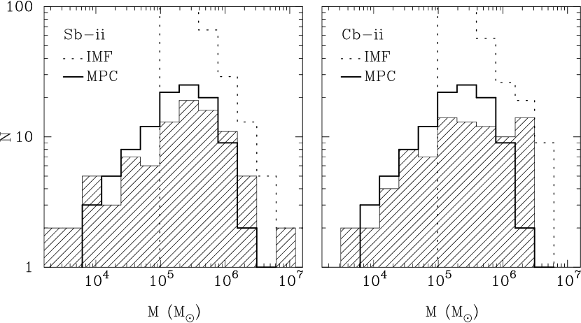
Figure 9.— Evolution of the mass function of model clusters from an initial power law (dotted histogram) to a peaked distribution at present (shaded histogram), including mass loss due to stellar evolution, two-body relaxation, and tidal shocks. Left panel: model Sb-ii, right panel: model Cb-ii. For comparison, the solid histogram shows the mass function of metal-poor globular clusters in the Galaxy.

4. Evolution of the Globular Cluster Mass Function

Using realistic cluster orbits and the specified $R_{h}-M$ relations, we now integrate equation (10) for the evolution of GCMF from $z=z_{f}$ to $z=0$. Figure 9 shows the transformation of the cluster mass function from an initial power law, $dN/dM\propto M^{-2}$, into a final peaked distribution for models Sb-ii and Cb-ii. High-mass clusters with $M\gtrsim 2\times 10^{5}\,\mathrm{M}_{\odot}$ approximately preserve the power-law shape of the IMF, while low-mass clusters are more easily affected by the mass loss due to stellar evolution, two-body relaxation, and tidal shocks.

We compare these model mass functions with the distribution of metal-poor (MPC, ${\rm[Fe/H]}<-0.8$) globular clusters in the Galaxy because they are the type of clusters described by our model (see § 2.5). We obtain $V$–band luminosities of the Galactic clusters from the current version of Harris’s catalog (Harris, 1996) and use a constant mass-to-light ratio, $M/L_{V}=3$ in solar units, to transform luminosities to stellar masses. The two plotted model mass functions are in excellent agreement with the observed GCMF of the Galactic metal-poor clusters.

We fit the model GCMF with a traditional lognormal function,
$dN/dM\propto\exp{[-(\log{M}-\log{M_{\rm peak}})^{2}/2\sigma^{2}]}\,dM$. The peak mass and the dispersion are very similar for both plotted models: $M_{\rm peak}=(2.9\pm 0.13)\times 10^{5}\,\mathrm{M}_{\odot}$, $\sigma=0.61\pm 0.10$ (model Sb-ii) and $M_{\rm peak}=(2.3\pm 0.13)\times 10^{5}\,\mathrm{M}_{\odot}$, $\sigma=0.66\pm 0.10$ (model Cb-ii). For the metal-poor Galactic clusters we find $M_{\rm peak}=2.1\times 10^{5}\,\mathrm{M}_{\odot}$ and $\sigma=0.51$. The observed and model distributions are statistically consistent with each other.

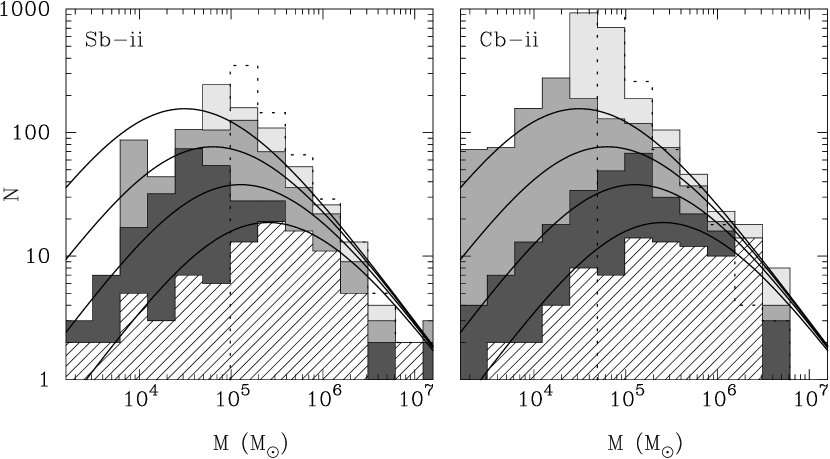
Figure 10.— Evolution of the mass function with time, beginning at $z=4$ (dotted histogram) and subsequently after 1.5 Gyr (light grey), 3 Gyr, 6 Gyr (dark grey), and 12 Gyr (shaded histogram, corresponds to the present epoch). Left panel: model Sb-ii, right panel: model Cb-ii. For comparison, solid lines (same in both panels) show the predicted evolution of the mass function in the model of Fall & Zhang (2001) at 1.5 Gyr, 3 Gyr, 6 Gyr, and 12 Gyr after cluster formation, from top to bottom.

To further quantify this agreement, we use a Kolmogorov-Smirnov (KS) test to calculate the probability of drawing the model GCMF and the observed GCMF from the same underlying distribution. Table 1 lists the results for all models we consider. The two models that we plot in Figure 9 and use to study the spatial and kinematic distributions have the highest KS probabilities: Sb-ii ($P_{KS}=0.24$) and Cb-ii ($P_{KS}=0.06$). In these models the initial half-mass density is the same for all massive clusters and it remains constant through time: $R_{h}(t)\propto M(t)^{1/3}$. A single epoch of formation is slightly preferred to the continuous formation scenario, but this difference is not statistically significant. In contrast, most of the other models are strongly inconsistent with the observed mass function of Galactic metal-poor clusters.

Recall that in setting the initial distribution of model clusters, we included only massive clusters with $M\geq 10^{5}\,\mathrm{M}_{\odot}$, as we expected all lower-mass clusters to be disrupted. We have verified this assumption and find that the lowest initial mass of the clusters that survive to $z=0$ are $3.8\times 10^{5}\,\mathrm{M}_{\odot}$ in model Sb-ii and $4.4\times 10^{5}\,\mathrm{M}_{\odot}$ in model Cb-ii. All of the low-mass clusters are destroyed by the present time.

Table 1 shows also the fractions of surviving model clusters by mass and by number, for clusters with $M>10^{5}\,\mathrm{M}_{\odot}$. In a single formation epoch model Sb-ii, only $f_{N}=0.16$ of the initial massive clusters survive until $z=0$, but they contain a higher fraction of the initial cluster mass, $f_{M}=0.46$. In the continuous formation model Cb-ii, both fractions are a factor of $3-4$ lower: $f_{N}=0.04$ and $f_{M}=0.16$. In the latter model, low-mass clusters are relatively more abundant at $z_{f}>4$, when the host galaxies are smaller than at $z_{f}=4$, and their subsequent rapid disruption results in the smaller surviving fractions.

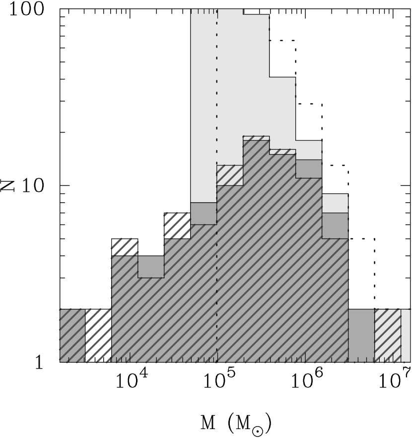
Figure 11.— Evolution of the mass function in model Sb-ii as a result of inclusion of different disruption processes: stellar evolution (light-grey histogram), two-body relaxation and evaporation (dark histogram), and tidal shocks (hatched histogram, final distribution).

Figure 10 shows the evolution of the cluster mass function with time, for the best models Sb-ii and Cb-ii. In model Sb-ii all clusters form at redshift $z=4$, but in model Cb-ii clusters form continuously beginning at $z=9$. To illustrate both formation scenarios in the same way, we plot the distribution of clusters in model Cb-ii at redshift $z=4$ (formed between $z=9$ and $z=4$) as the “initial” GCMF. This epoch corresponds to a cosmic time of 1.5 Gyr, which is almost exactly 12 Gyr ago, in our adopted cosmology. The sequence of histograms displays the progression of the GCMF at four successive epochs (0, 1.5, 6, and 12 Gyr) after $z=4$.

For comparison, Figure 10 shows also the mass functions predicted by the model of Fall & Zhang (2001) at the same epochs. Fall & Zhang (2001) consider several initial forms of the GCMF, several kinematic distributions of the clusters in the Galaxy, and several prescriptions for disk shocking, and solve equation (10) under these different assumptions. They also keep the half-mass density $M/R_{h}^{3}$ constant as a function of time and find that this is the best way to reproduce the observed GCMF, in agreement with our conclusions. We select one of their models (top left panel of their Fig. 3), which is the closest match to our models. This model has an initial power-law GCMF with the slope $\alpha=2$ and a single epoch of cluster formation, which we assume equal to $z=4$. We normalize their model to have the same initial number of clusters with $M>10^{5}\,\mathrm{M}_{\odot}$ as in our model in each of the panels of Figure 10.

We find a reasonable agreement of our GCMF with the prediction of Fall & Zhang (2001) at late times. At 1.5 Gyr after cluster formation, our clusters are less affected by the dynamical evolution, especially in the continuous formation model Cb-ii. Note that although our models do not include clusters with $M<10^{5}\,\mathrm{M}_{\odot}$ initially, this does not affect the comparison in the range $M=10^{5}-4\times 10^{5}\,\mathrm{M}_{\odot}$, where our models predict somewhat slower evolution than the model of Fall & Zhang (2001). The final distributions in our two best models are similar to each other and to the prediction of Fall & Zhang (2001). The peak of the log-normal fit is $\log{M_{\rm peak}}=5.46$ (Sb-ii) and 5.37 (Cb-ii) vs. 5.42 (FZ), and the dispersion is 0.61 (Sb-ii) and 0.66 (Cb-ii) vs. 0.63 (FZ). Note that although we use the parameters of the log-normal function for the ease of comparison between different models and between models and observations, the mass function below the peak is better described by a power law, $dN/d\log{M}\propto M$ or $dN/dM=\mbox{const}$ (see Fall & Zhang, 2001).

Figure 11 provides insight into the effects of each of the disruption mechanisms separately. Mass loss due to stellar evolution simply shifts the whole mass function to the left. The relative importance of two-body relaxation and tidal shocks depends on the $R_{h}(M)$ relation. Let us write this relation in a general power-law form, $R_{h}\propto M^{\delta}$. Then the ratio of the mass loss rates is $\nu_{\rm ev}/\nu_{\rm sh}\propto M^{1/2}R_{h}^{-9/2}\propto M^{1/2-9\delta/2}$. Unless $\delta<1/9$ (in the plotted model Sb-ii, $\delta=1/3$), two-body relaxation is more effective in low-mass clusters, and tidal shocks are more effective in high-mass clusters. The evolution of the $R_{h}(M)$ relation with time may also affect the balance between the two processes. The dark histogram in Figure 11 shows how the inclusion of the evaporation due to two-body relaxation removes a large number of low-mass clusters and turns the mass function into a peaked distribution. Inclusion of tidal shocks affects mainly the most massive clusters and reduces their surviving fraction.

Figure 12.— Models that fail to reproduce the observed mass function of metal-poor globular clusters: with $R_{h}(t)={\rm const}$ (Sa-i, left), and with $R_{h}(t)\propto M(t)$ with single epoch of formation (Sb-iii, middle) and continuous formation (Ca-iii, right). Normalization of the initial model distribution is such that the number of clusters at $z=0$ is close to the observed number of clusters in the Galaxy.

Our results agree with previous studies of the evolution of the cluster mass function, which found that almost any initial function can be turned into a peaked distribution as a consequence of the dynamical evolution. The new result of our study is that not all initial conditions and not all evolutionary scenarios are consistent with the observed mass function.

Figure 12 provides three examples. In the first (top left panel, model Sa-i), the half-mass radius is kept fixed at the median value for Galactic globulars, $R_{h}=2.4$ pc, for clusters of all masses and at all times. The median density $M(t)/R_{h}^{3}$ decreases as the clusters lose mass. Therefore, two-body relaxation becomes less efficient and spares many low-mass clusters, while tidal shocks become more efficient and disrupt most high-mass clusters. The final distribution is severely skewed towards small clusters. In the second example (top right panel, model Sb-iii), the median density is initially fixed, as in our best models, but the half-mass radius is assumed to evolve in proportion to the mass, $R_{h}(t)\propto M(t)$. In this case the cluster density increases with time. As a result, all of the low-mass clusters are disrupted by the enhanced two-body relaxation, while the high-mass clusters are unaffected by the weakened tidal shocks. The final distribution is skewed towards massive clusters. In the third example (bottom left panel, model Ca-iii), the initial half-mass radius is the same for all clusters but then varies as $R_{h}(t)\propto M(t)$. In this model, which assumes a continuous formation scenario from $z_{f}=9$ to $z_{f}=3$, the median cluster density again increases with time and all of the low-mass clusters are destroyed by two-body relaxation. The initial relation $R_{h}(0)$ vs. $M(0)$ does not appear to be as important for the final mass function as the evolution of this relation with time, $R_{h}(t)$ vs. $M(t)$.

5. Radial Variation of the Globular Cluster Mass Function

A generic prediction of the dynamical disruption models is that the evolution is faster in the inner parts of the galaxy, where the stronger tidal field enhances both two-body relaxation and tidal shocks. As a result, the low-mass part of the mass function should be depleted more strongly in the inner regions, causing an apparent peak mass to be higher than in the outer regions (Ostriker & Gnedin, 1997). Such radial dependence of the mass function is marginally present in the Galaxy (Gnedin, 1997) and more clearly in M31 (Barmby et al., 2001), but it has not been detected in other extragalactic systems. This lack of the observed radial variation has led Fall & Zhang (2001) to consider anisotropic cluster orbits, which may suppress radial dependence of the disruption processes.

Our best model Sb-ii does not predict a significant radial variation of the mass. To investigate this, we have divided the model sample into two subsamples, splitting them at a distance $r=30$ kpc from the center. The inner sample has 30 clusters, the outer 70 clusters. (Had we split the model sample into two equal parts, the dividing distance would be 90 kpc, too large to expect any differences in the dynamical evolution.) A lognormal fit to the distribution of the inner clusters gives the peak mass and dispersion $\log{M_{\rm peak}}=5.56\pm 0.20$, $\sigma=0.44\pm 0.17$, while for the outer clusters $\log{M_{\rm peak}}=5.39\pm 0.17$, $\sigma=0.82\pm 0.13$, respectively. The KS probability of the two subsamples being drawn from the same distribution is extremely high, $P_{KS}=0.99$.

The mass functions of the model subsamples are consistent, within the 1$\sigma$ uncertainties, with the mass functions of the metal-poor Galactic clusters, split in two equal-size parts at 7 kpc: $\log{M_{\rm peak}}=5.35\pm 0.09$, $\sigma=0.40\pm 0.07$ (inner clusters), and $\log{M_{\rm peak}}=5.31\pm 0.16$, $\sigma=0.61\pm 0.11$ (outer clusters). Note however the caveat that the assumed dividing radius for our model clusters (30 kpc) is significantly larger than that for the Galactic clusters (7 kpc). This is partially, but not entirely, offset by the fact that our model galaxy is twice the size of the Milky Way and the extent of its globular cluster system is expected to scale accordingly.

The lack of a significant radial gradient in our best models is due to the contribution of tidal shocks being sub-dominant compared to the contribution of two-body relaxation. Under our assumption that the median density $M/R_{h}^{3}$ is constant and does not depend on the position in the galaxy, the rate of cluster mass loss due to two-body relaxation alone is independent of location. The rate of tidal shocks does depend on the position and on cluster orbits, but because their contribution is relatively small, the resulting radial gradient is small as well. We have verified this hypothesis by looking at one of the failed models (Sa-i), where tidal shocks are strongly enhanced compared to two-body relaxation. This model shows a clear and strong radial dependence of the mass function. Therefore, the lack of the gradient in our best models may be more of a product of the initial set-up rather than a model prediction, but it does show that our best models successfully pass this observational test.

6. Conclusions

We have verified the hypothesis that the properties of globular clusters formed within high-redshift disk galaxies are consistent with the observed properties of Galactic metal-poor clusters. After calculating the orbits of model clusters in the time-variable gravitational potential of a Milky Way-sized galaxy, we find that at present the orbits are isotropic in the inner 50 kpc and preferentially radial at larger distances. All clusters located outside 10 kpc from the center formed in satellite galaxies, some of which are now tidally disrupted. The spatial distribution of model clusters is spheroidal, with a spherical density profile that can be fit by a power law with the slope $\gamma\approx 2.7$, consistent with the observations of Galactic metal-poor clusters.

Two-body relaxation dominates over other disruption processes and drives the evolution of the cluster mass function from an initial power law to the observed peaked distribution. The evolution of the mass function in our best models is in close agreement with the models of Fall & Zhang (2001) at late times and is somewhat slower at early times. We find no significant variation of the mass function with radius, which is largely due to the rate of two-body relaxation being independent of cluster location. Knowledge of realistic orbits is important for accurate calculations of the globular cluster evolution, although we find that tidal shocks play only a moderate role in cluster disruption. Therefore, any inaccuracies in orbit calculations are not expected to significantly affect the evolution of the mass function.

Interestingly, we find that not all initial conditions and not all evolution scenarios are consistent with the observed mass function. If the half-mass radius remains constant throughout the evolution instead of decreasing with mass, the rate of two-body relaxation is suppressed and the final mass distribution is skewed towards too many low-mass clusters. On the other hand, if the half-mass radius decreases too quickly, proportionally to the mass, then two-body relaxation is too efficient and there are no low-mass clusters left. The successful models (Sb-ii and Cb-ii) require the average cluster density, $M/R_{h}^{3}$, to be constant initially for clusters of all mass, as in the model of Kravtsov & Gnedin (2005), and to remain constant with time.

We have investigated two formation scenarios. Synchronous formation of all clusters at a single epoch ($z=4$) and continuous formation over a span of 1.6 Gyr (between $z=9$ and $z=3$) both appear consistent with the observed mass function, spatial and kinematic distributions of the Galactic globular clusters. However, clusters that formed at later epochs have more extended spatial distribution than the clusters that formed at early epochs. This is expected for objects that trace the distribution of high-density peaks in hierarchical galaxy formation. If additional clusters form after $z=3$, they are expected to have a shallower density profile than the clusters we study in this paper. The profile of our clusters is consistent with, but is already somewhat shallower than the profile of the Galactic metal-poor clusters. Therefore, we do not expect a significant fraction of metal-poor clusters to have formed after $z=3$. Metal-rich clusters, associated with the Galactic disk, are not included in our present formation model and will be studied in future work.

In online Tables 2 and 3 we provide catalogs of the physical properties of model clusters that survive to the present time, for the best models Sb-ii and Cb-ii, respectively. These catalogs can be used to compare with other models of the dynamical evolution, to study selection effects in extragalactic systems, and to model the kinematics of globular cluster systems.

Table 1

Model	$R_{h}(0)$	$R_{h}(t)$	$\gamma$	$\langle e\rangle$	$f_{M}$	$f_{N}$	$\log{M_{\rm peak}}$	$\sigma$	$P_{KS}$
Sa-i	const	const	2.6	0.53	0.29	0.54	3.76	1.02	$<10^{-10}$
Sa-ii	const	$M(t)^{1/3}$	2.6	0.54	0.40	0.20	5.02	0.68	$2\times 10^{-4}$
Sa-iii	const	$M(t)$	2.6	0.58	0.38	0.05	5.98	0.66	$7\times 10^{-8}$
Sb-i	$M(0)^{1/3}$	const	2.6	0.53	0.45	0.27	4.97	0.95	0.0035
Sb-ii	$M(0)^{1/3}$	$M(t)^{1/3}$	2.7	0.53	0.46	0.16	5.46	0.61	0.24
Sb-iii	$M(0)^{1/3}$	$M(t)$	2.6	0.57	0.54	0.09	5.88	0.52	$4\times 10^{-10}$
Ca-i	const	const	2.5	0.54	0.15	0.43	1.96	1.40	$<10^{-10}$
Ca-ii	const	$M(t)^{1/3}$	2.7	0.53	0.11	0.05	5.14	0.71	0.023
Ca-iii	const	$M(t)$	2.7	0.57	0.16	0.02	6.04	0.62	$<10^{-10}$
Cb-i	$M(0)^{1/3}$	const	2.8	0.52	0.17	0.08	4.88	0.83	$3\times 10^{-4}$
Cb-ii	$M(0)^{1/3}$	$M(t)^{1/3}$	2.7	0.52	0.15	0.04	5.37	0.66	0.063
Cb-iii	$M(0)^{1/3}$	$M(t)$	2.7	0.56	0.21	0.03	6.08	0.51	$<10^{-10}$

Table 2Catalog of clusters in model Sb-ii.

$z_{\rm f}$	$\log{M}$	$\log{M_{i}}$	$R_{h}$	$R_{h,i}$	$r$	$r_{i}$	$\log{M_{{\rm halo},i}}$	$x$	$y$	$z$	$v_{x}$	$v_{y}$	$v_{z}$
4.0	5.72	6.10	2.5	3.4	4.2	0.7	10.9	$-$3.8	$-$1.6	$-$0.6	$-$25.4	$-$12.3	$-$28.5
4.0	5.34	5.91	1.9	2.9	6.4	1.1	10.9	$-$0.4	$-$2.9	$-$5.7	$-$28.5	$-$144.7	$-$21.7
4.0	3.99	5.72	0.7	2.5	1.4	1.2	10.9	1.1	0.5	0.7	57.5	4.0	18.6
4.0	5.15	5.87	1.6	2.8	1.4	1.5	10.9	0.8	0.1	1.1	23.1	112.9	26.8
4.0	6.18	6.43	3.6	4.3	0.4	1.8	10.9	$-$0.4	$-$0.1	$-$0.0	$-$110.2	$-$3.7	$-$94.9
							…

Note. — Columns are: $z_{f}$ – redshift of formation, $\log{M}$ – present cluster mass in $\mathrm{M}_{\odot}$, $\log{M_{i}}$ – initial mass, $R_{h}$ – present half-mass radius of the cluster in pc, $R_{h,i}$ – initial half-mass radius, $r$ – present distance to the center of the main galaxy in kpc, $r_{i}$ – initial distance to the center of the main galaxy, $\log{M_{{\rm halo},i}}$ – mass of the host galaxy at the time of cluster formation in $\mathrm{M}_{\odot}$, $x$, $y$, $z$ – present coordinates of the cluster with respect to the center of the main galaxy in kpc, $v_{x}$, $v_{y}$, $v_{z}$ – present velocities of the cluster in km s^-1. Complete table is available online.

Table 3Catalog of clusters in model Cb-ii.

$z_{\rm f}$	$\log{M}$	$\log{M_{i}}$	$R_{h}$	$R_{h,i}$	$r$	$r_{i}$	$\log{M_{{\rm halo},i}}$	$x$	$y$	$z$	$v_{x}$	$v_{y}$	$v_{z}$
6.2	4.91	5.83	1.3	2.7	2.3	1.4	10.5	0.7	2.1	0.7	35.3	32.5	37.7
5.6	4.96	5.83	1.4	2.7	3.6	2.8	10.5	0.6	3.5	1.2	123.9	25.4	64.7
5.4	5.01	5.83	1.5	2.7	2.6	0.7	10.6	$-$1.3	$-$1.9	$-$0.7	$-$94.4	$-$30.2	$-$34.0
5.2	5.75	6.13	2.6	3.4	9.8	1.7	10.7	4.2	7.7	2.7	42.5	7.9	84.2
5.0	5.68	6.08	2.4	3.3	17.3	6.5	10.7	3.5	16.5	4.8	79.0	54.0	10.1
							…

Note. — Columns are the same as in Table 2. Complete table is available online.

References

- Anders et al. (2004) Anders, P., de Grijs, R., Fritze-v. Alvensleben, U., & Bissantz, N. 2004, MNRAS, 347, 17
- Barmby et al. (2001) Barmby, P., Huchra, J. P., & Brodie, J. P. 2001, AJ, 121, 1482
- Binney & Tremaine (1987) Binney, J. & Tremaine, S. 1987, Galactic Dynamics (Princeton, NJ, Princeton University Press)
- Chandrasekhar (1943) Chandrasekhar, S. 1943, ApJ, 97, 255
- Chernoff et al. (1986) Chernoff, D. F., Kochanek, C. S., & Shapiro, S. L. 1986, ApJ, 309, 183
- Chernoff & Weinberg (1990) Chernoff, D. F. & Weinberg, M. D. 1990, ApJ, 351, 121
- Colín et al. (2000) Colín, P., Klypin, A. A., & Kravtsov, A. V. 2000, ApJ, 539, 561
- Cote et al. (1998) Cote, P., Marzke, R. O., & West, M. J. 1998, ApJ, 501, 554
- de Grijs et al. (2003) de Grijs, R., Anders, P., Bastian, N., Lynds, R., Lamers, H. J. G. L. M., & O’Neil, E. J. 2003, MNRAS, 343, 1285
- de Grijs et al. (2004) de Grijs, R., Smith, L. J., Bunker, A., Sharp, R. G., Gallagher, J. S., Anders, P., Lançon, A., O’Connell, R. W., & Parry, I. R. 2004, MNRAS, 352, 263
- Dirsch et al. (2005) Dirsch, B., Schuberth, Y., & Richtler, T. 2005, A&A, 433, 43
- Engargiola et al. (2003) Engargiola, G., Plambeck, R. L., Rosolowsky, E., & Blitz, L. 2003, ApJS, 149, 343
- Fall et al. (2005) Fall, S. M., Chandar, R., & Whitmore, B. C. 2005, ApJ, 631, L133
- Fall & Zhang (2001) Fall, S. M. & Zhang, Q. 2001, ApJ, 561, 751
- Forbes et al. (2006) Forbes, D. A., Sánchez-Blázquez, P., Phan, A. T. T., Brodie, J. P., Strader, J., & Spitler, L. 2006, MNRAS, 366, 1230
- Forte et al. (2005) Forte, J. C., Faifer, F., & Geisler, D. 2005, MNRAS, 357, 56
- Frenk & White (1980) Frenk, C. S. & White, S. D. M. 1980, MNRAS, 193, 295
- Gnedin (1997) Gnedin, O. Y. 1997, ApJ, 487, 663
- Gnedin (2003) —. 2003, in Extragalactic Globular Cluster Systems, ed. M. Kissler-Patig (Springer), p. 224; astro-ph/0210556
- Gnedin et al. (1999a) Gnedin, O. Y., Hernquist, L., & Ostriker, J. P. 1999a, ApJ, 514, 109
- Gnedin et al. (2004) Gnedin, O. Y., Kravtsov, A. V., Klypin, A. A., & Nagai, D. 2004, ApJ, 616, 16
- Gnedin et al. (1999b) Gnedin, O. Y., Lee, H. M., & Ostriker, J. P. 1999b, ApJ, 522, 935
- Gnedin & Ostriker (1997) Gnedin, O. Y. & Ostriker, J. P. 1997, ApJ, 474, 223
- Gnedin & Ostriker (1999) —. 1999, ApJ, 513, 626
- Harris et al. (2004) Harris, G. L. H., Harris, W. E., & Geisler, D. 2004, AJ, 128, 723
- Harris (1986) Harris, W. E. 1986, AJ, 91, 822
- Harris (1996) —. 1996, AJ, 112, 1487
- Harris (2001) Harris, W. E. 2001, in Star Clusters, Saas-Fee Advanced Course 28. Lecture Notes 1998, Swiss Society for Astrophysics and Astronomy. Edited by L. Labhardt and B. Binggeli (Springer-Verlag:Berlin), 223–408
- Hénon (1961) Hénon, M. 1961, Annales d’Astrophysique, 24, 369
- Ho & Filippenko (1996) Ho, L. C. & Filippenko, A. V. 1996, ApJ, 472, 600
- Holtzman et al. (1992) Holtzman, J. A., Faber, S. M., Shaya, E. J., Lauer, T. R., Groth, J., Hunter, D. A., Baum, W. A., Ewald, S. P., Hester, J. J., Light, R. M., Lynds, C. R., O’Neil, E. J., & Westphal, J. A. 1992, AJ, 103, 691
- Hurley et al. (2000) Hurley, J. R., Pols, O. R., & Tout, C. A. 2000, MNRAS, 315, 543
- Keto et al. (2005) Keto, E., Ho, L. C., & Lo, K. Y. 2005, astro-ph/0508519
- Kissler-Patig (1997) Kissler-Patig, M. 1997, A&A, 319, 83
- Klypin et al. (1999) Klypin, A., Gottlöber, S., Kravtsov, A. V., & Khokhlov, A. M. 1999, ApJ, 516, 530
- Klypin et al. (2002) Klypin, A., Zhao, H., & Somerville, R. S. 2002, ApJ, 573, 597
- Kravtsov (1999) Kravtsov, A. V. 1999, PhD thesis, New Mexico State University
- Kravtsov & Gnedin (2005) Kravtsov, A. V. & Gnedin, O. Y. 2005, ApJ, 623, 650
- Kravtsov et al. (2004) Kravtsov, A. V., Gnedin, O. Y., & Klypin, A. A. 2004, ApJ, 609, 482
- Kravtsov et al. (1997) Kravtsov, A. V., Klypin, A. A., & Khokhlov, A. M. 1997, ApJS, 111, 73
- Kroupa (2001) Kroupa, P. 2001, MNRAS, 322, 231
- Kundic & Ostriker (1995) Kundic, T. & Ostriker, J. P. 1995, ApJ, 438, 702
- Lahav et al. (1991) Lahav, O., Lilje, P. B., Primack, J. R., & Rees, M. J. 1991, MNRAS, 251, 128
- Larsen (2002) Larsen, S. S. 2002, AJ, 124, 1393
- Macciò et al. (2006) Macciò, A. V., Moore, B., Stadel, J., & Diemand, J. 2006, MNRAS, 366, 1529
- Mengel et al. (2002) Mengel, S., Lehnert, M. D., Thatte, N., & Genzel, R. 2002, A&A, 383, 137
- Mengel et al. (2005) —. 2005, A&A, 443, 41
- Miyamoto & Nagai (1975) Miyamoto, M. & Nagai, R. 1975, PASJ, 27, 533
- Moore et al. (2006) Moore, B., Diemand, J., Madau, P., Zemp, M., & Stadel, J. 2006, MNRAS, 368, 563
- Murali & Weinberg (1997a) Murali, C. & Weinberg, M. D. 1997a, MNRAS, 291, 717
- Murali & Weinberg (1997b) —. 1997b, MNRAS, 288, 767
- Murali & Weinberg (1997c) —. 1997c, MNRAS, 288, 749
- Nagai & Kravtsov (2005) Nagai, D. & Kravtsov, A. V. 2005, ApJ, 618, 557
- Navarro et al. (1997) Navarro, J. F., Frenk, C. S., & White, S. D. M. 1997, ApJ, 490, 493
- O’Connell et al. (1995) O’Connell, R. W., Gallagher, J. S., Hunter, D. A., & Colley, W. N. 1995, ApJ, 446, L1
- Ostriker & Gnedin (1997) Ostriker, J. P. & Gnedin, O. Y. 1997, ApJ, 487, 667
- Ostriker et al. (1972) Ostriker, J. P., Spitzer, L. J., & Chevalier, R. A. 1972, ApJ, 176, L51
- Peñarrubia & Benson (2005) Peñarrubia, J. & Benson, A. J. 2005, MNRAS, 364, 977
- Puzia et al. (2004) Puzia, T. H., Kissler-Patig, M., Thomas, D., Maraston, C., Saglia, R. P., Bender, R., Richtler, T., Goudfrooij, P., & Hempel, M. 2004, A&A, 415, 123
- Rhode & Zepf (2003) Rhode, K. L. & Zepf, S. E. 2003, AJ, 126, 2307
- Rhode & Zepf (2004) —. 2004, AJ, 127, 302
- Salpeter (1955) Salpeter, E. E. 1955, ApJ, 121, 161
- Scalo (1986) Scalo, J. M. 1986, Fundamentals of Cosmic Physics, 11, 1
- Spitzer (1987) Spitzer, L. 1987, Dynamical Evolution of Globular Clusters (Princeton: Princeton University Press)
- Thomas (1989) Thomas, P. 1989, MNRAS, 238, 1319
- Vesperini et al. (2003) Vesperini, E., Zepf, S. E., Kundu, A., & Ashman, K. M. 2003, ApJ, 593, 760
- Weinberg et al. (2006) Weinberg, D. H., Colombi, S., Davé, R., & Katz, N. 2006, astro-ph/0604393
- Whitmore & Schweizer (1995) Whitmore, B. C. & Schweizer, F. 1995, AJ, 109, 960
- Whitmore et al. (1993) Whitmore, B. C., Schweizer, F., Leitherer, C., Borne, K., & Robert, C. 1993, AJ, 106, 1354
- Wilson et al. (2003) Wilson, C. D., Scoville, N., Madden, S. C., & Charmandaris, V. 2003, ApJ, 599, 1049
- Zentner & Bullock (2003) Zentner, A. R. & Bullock, J. S. 2003, ApJ, 598, 49
- Zepf et al. (1999) Zepf, S. E., Ashman, K. M., English, J., Freeman, K. C., & Sharples, R. M. 1999, AJ, 118, 752
- Zhang & Fall (1999) Zhang, Q. & Fall, S. M. 1999, ApJ, 527, L81