Spin exchange rates in electron-hydrogen collisions

Abstract

The spin temperature of neutral hydrogen, which determines the 21 cm optical depth and brightness temperature, is set by the competition between radiative and collisional processes. In the high-redshift intergalactic medium, the dominant collisions are typically those between hydrogen atoms. However, collisions with electrons couple much more efficiently to the spin state of hydrogen than do collisions with other hydrogen atoms and thus become important once the ionized fraction exceeds $\sim 1\%$. Here we compute the rate at which electron-hydrogen collisions change the hydrogen spin. Previous calculations included only $S$-wave scattering and ignored resonances near the $n=2$ threshold. We provide accurate results, including all partial wave terms through the $F$-wave, for the de-excitation rate at temperatures $T_{K}\la 1.5\times 10^{4}\mbox{ K}$; beyond that point, excitation to $n\geq 2$ hydrogen levels becomes significant. Accurate electron-hydrogen collision rates at higher temperatures are not necessary, because collisional excitation in this regime inevitably produces Ly$\alpha$ photons, which in turn dominate spin exchange when $T_{K}\ga 6200\mbox{ K}$ even in the absence of radiative sources. Our rates differ from previous calculations by several percent over the temperature range of interest. We also consider some simple astrophysical examples where our spin de-excitation rates are useful.

1 Introduction

The 21 cm transition is potentially a powerful probe of the pre-reionization intergalactic medium (IGM) because of the enormous amount of neutral hydrogen in the Universe at that time (Field, 1958; Scott & Rees, 1990; Madau et al., 1997). It can teach us about reionization, the formation of the first structures and the first galaxies, and even the “dark ages” before these objects formed (Furlanetto et al. 2006, and references therein). It is therefore crucial to understand the fundamental physics underlying the 21 cm transition. One critical aspect is the spin temperature, which is determined by the competition between the scattering of cosmic microwave background (CMB) photons, the scattering of Ly$\alpha$ photons (Wouthuysen, 1952; Field, 1958), and collisions. When CMB scattering dominates, the IGM remains invisible because the spin temperature approaches that of the CMB (which is used as a backlight).

Before star formation commences, collisions are the only way to break this degeneracy. The total coupling rate is determined by collisions both with other hydrogen atoms and with electrons. At the low residual electron fraction expected after cosmological recombination (Seager et al., 1999), H–H collisions dominate. Spin exchange in such interactions has received a great deal of attention over the years (Purcell & Field, 1956; Smith, 1966; Allison & Dalgarno, 1969; Zygelman, 2005; Hirata & Sigurdson, 2006). Such collisions suffice to couple the spin temperature $T_{S}$ to the kinetic temperature $T_{K}$ at high densities, when $z\ga 50$ (Loeb & Zaldarriaga, 2004). However, the spin exchange rate in these collisions falls dramatically at $T_{K}\la 100\mbox{ K}$; coupled with the declining density, such interactions become ineffective at lower redshifts. H–e^- collisions have received much less attention. However, at fixed temperature, free electrons move at much higher velocities than do hydrogen atoms, and are thus much more efficient at spin exchange on a per-particle basis. If the mean ionized fraction is $\bar{x}_{i}\ga 0.01$, they can play a significant role in the coupling. This situation can occur if, for example, X-rays from the first quasars or star-forming galaxies create a warm, partially-ionized medium (Oh, 2001; Venkatesan et al., 2001; Ricotti & Ostriker, 2004; Ricotti et al., 2005; Nusser, 2005; Kuhlen & Madau, 2005; Kuhlen et al., 2006), or if the decay or annihilation of exotic particles deposits a significant amount of energy into the IGM (Chen & Kamionkowski, 2004; Pierpaoli, 2004; Shchekinov & Vasiliev, 2006; Furlanetto et al., 2006).

The spin de-excitation rate in H–e^- collisions, which we will denote $\kappa_{10}$, obviously depends on the detailed scattering properties of these collisions. Over the past several decades, this interaction has received a great deal of attention as a model problem for electron-atom interactions (e.g., Massey & Moiseiwitch 1951; Schwartz 1961; Temkin 1962; Burke & Schey 1962a; Poet 1978; Bray et al. 2002). At IGM temperatures $T_{K}\la 10^{4}\mbox{ K}$, most electrons have energies below the threshold to excite the $n=2$ level, and the dominant mechanism of spin de-excitation is electron-electron spin exchange. Although this regime has been particularly well-studied, it has only been solved in full nonrelativistic detail relatively recently. The latest spin exchange calculation (Smith, 1966) used the scattering phase shifts computed numerically by Schwartz (1961). While accurate, these included only $S$-wave scattering and neglected both higher-order partial waves and H^- resonances near the $n=2$ threshold (which were not resolved by the numerical algorithm). Both of these issues have been solved over the intervening four decades (see, e.g., Wang & Callaway 1993, 1994 for a recent calculation). Our goal is to recalculate $\kappa_{10}$ in light of these newer phase shifts.

Higher-order partial waves become significant at $T_{K}\ga 1000\mbox{ K}$; if X-ray heating in the early Universe is strong, then these temperatures can be achieved easily (Furlanetto, 2006). We therefore examine the high-temperature limit in some detail. Our calculation breaks down once collisional electronic excitation (and ionization) become important. We will show that, above $T_{K}\sim 1.5\times 10^{4}\mbox{ K}$, direct spin de-excitation by scattering above the $n=2$ threshold cannot be ignored. Although such interactions are difficult to model – because of the wide array of possible transitions – in practice this regime is relatively unimportant. In the low-density IGM, collisional excitation to the $2p$ and higher levels is followed rapidly by radiative de-excitation, producing a Ly$\alpha$ background. We show that this background inevitably dominates the spin temperature coupling at $T_{K}\ga 6200\mbox{ K}$ (assuming a thermal distribution of electrons). The crossover can occur at smaller temperatures if a non-thermal population of fast electrons exists (produced, for example, by X-rays; Chen & Miralda-Escude 2006; Chuzhoy et al. 2006).

The remainder of this paper is organized as follows. In §2, we briefly review the 21 cm transition. Our main results are contained in §3, where we examine various mechanisms for spin de-excitation, consider the high-temperature limit, and calculate the spin de-excitation rates for H–e^- collisions. We present some simple astrophysical applications in §4, and we conclude in §5.

In our numerical calculations, we assume a cosmology with $\Omega_{m}=0.26$, $\Omega_{\Lambda}=0.74$, $\Omega_{b}=0.044$, $H=100h\mbox{ km s${}^{-1}$ Mpc${}^{-1}$}$ (with $h=0.74$), $n=0.95$, and $\sigma_{8}=0.8$, consistent with the most recent measurements (Spergel et al., 2006), although we have increased $\sigma_{8}$ from the best-fit WMAP value in order to improve agreement with weak-lensing data.

2 The 21 cm Transition

We review the relevant characteristics of the 21 cm transition here; we refer the interested reader to Furlanetto et al. (2006) for a more comprehensive discussion. The 21 cm brightness temperature (relative to the CMB) of a patch of the IGM is

$$\delta T_{b} = 27\,x_{\rm HI}\,(1+\delta)\,\left(\frac{\Omega_{b}h^{2}}{0.023}\right)\left(\frac{0.15}{\Omega_{m}h^{2}}\,\frac{1+z}{10}\right)^{1/2}$$ (1)

$$\times\left(\frac{T_{S}-T_{\gamma}}{T_{S}}\right)\,\left[\frac{H(z)/(1+z)}{{\rm d}v_{\parallel}/{\rm d}r_{\parallel}}\right]\mbox{ mK},$$

where $\delta$ is the fractional overdensity, $x_{\rm HI}$ is the neutral fraction, $x_{i}=1-x_{\rm HI}$ is the ionized fraction, $T_{S}$ is the spin temperature, $T_{\gamma}$ is the CMB temperature, and ${\rm d}v_{\parallel}/{\rm d}r_{\parallel}$ is the gradient of the proper velocity along the line of sight. The last factor accounts for redshift-space distortions (Bharadwaj & Ali, 2004; Barkana & Loeb, 2005).

The spin temperature $T_{S}$ is determined by competition between scattering of CMB photons, scattering of UV photons (Wouthuysen, 1952; Field, 1958), and collisions (Purcell & Field, 1956). In equilibrium,

$$T_{S}^{-1}=\frac{T_{\gamma}^{-1}+x_{c}T_{K}^{-1}+x_{\alpha}T_{c}^{-1}}{1+x_{c}+x_{\alpha}}.$$ (2)

Here $x_{c}$ is the total collisional coupling coefficient, including both H–H and H–e^- collisions. We will break the total coupling into two components, $x_{c}^{\rm HH}$ and $x_{c}^{\rm eH}$, with obvious meanings. The coefficient from H–e^- collisions is

$$x_{c}^{\rm eH}=\frac{n_{e}\kappa_{10}T_{\star}}{A_{10}T_{\gamma}},$$ (3)

where $n_{e}$ is the local electron density, $T_{\star}\equiv h\nu_{21}/k_{B}=0.068\mbox{ K}$, $\nu_{21}$ is the frequency of the 21 cm line, and $A_{10}$ is the Einstein-$A$ coefficient for that transition. The last part of equation (2) describes the Wouthuysen-Field effect, in which the absorption and re-emission of Ly$\alpha$ photons mixes the hyperfine states. The coupling coefficient is (Chen & Miralda-Escudé, 2004)

$$x_{\alpha}=1.81\times 10^{11}(1+z)^{-1}S_{\alpha}J_{\alpha},$$ (4)

where $S_{\alpha}\leq 1$ describes the detailed atomic physics of the scattering process and $J_{\alpha}$ is the background flux at the Ly$\alpha$ frequency (ignoring scattering) in units of cm^-2 s^-1 Hz^-1 sr^-1; the Wouthuysen-Field effect becomes efficient when there is $\sim 0.1$ photon per baryon near this frequency. It couples $T_{S}$ to an effective color temperature $T_{c}$ (in most circumstances, $T_{c}\approx T_{K}$; Field 1959). Several estimates of $S_{\alpha}$ and $T_{c}$ exist in the literature (Chen & Miralda-Escudé, 2004; Hirata, 2006; Chuzhoy & Shapiro, 2005; Furlanetto & Pritchard, 2006).

3 Electron-Hydrogen Collisions

3.1 Mechanisms of collisional spin de-excitation

In principle there are five distinct collisional mechanisms that can cause spin de-excitation. The existing literature has addressed only one of these, electron spin exchange. As we intend to increase the accuracy to which $\kappa_{10}$ is known, we will first reconsider the relative magnitudes of each mechanism. We will then calculate spin de-excitation cross sections and compare them to previous results.

3.1.1 Electron-electron spin exchange

Electron-electron spin exchange refers to the process by which the spin of the incoming electron is exchanged with that of the atomic electron. One such collision could be represented schematically by

$$\alpha(s)+\beta(a)\alpha(p)\rightarrow\beta(s)+\alpha(a)\alpha(p),$$ (5)

where $\alpha$ and $\beta$ refer to the Pauli spin states of spin-$\frac{1}{2}$ particles, $s$ and $a$ refer to the scattering and atomic electrons, respectively, and $p$ refers to the proton. In this collision, a singlet hydrogen atom is converted into a triplet hydrogen atom by spin exchange. Including all possible spin permutations of this collision leads to an expression for the spin de-excitation cross section. (For a more detailed discussion of spin exchange see Mott & Massey 1965 and Condon & Shortley 1963.)

Ignoring all relativistic interactions and non-central forces, the spin-exchange-mediated spin de-excitation cross section can be calculated relatively simply. (Interactions which violate these assumptions will be discussed below in §3.1.2 and §3.1.3.) We begin with the time-independent Schrödinger equation, which may be written

$$\hat{H}\Psi({{\bf x}},{{\bf y}})=E\Psi({\bf x},{{\bf y}}),$$ (6)

where, in atomic units,

$$\hat{H}=-\nabla^{2}_{{\bf x}}-\nabla^{2}_{{\bf y}}-\frac{2}{|{\bf x}|}-\frac{2}{|{\bf y}|}+\frac{2}{|{{\bf x}}-{{\bf y}}|},$$ (7)

$\Psi$ is the total wavefunction, and ${{\bf x}}$ and ${{\bf y}}$ label the positions of the two electrons. The Pauli exclusion principle demands that

$$\Psi({{\bf x}},{{\bf y}})=\pm\Psi({{\bf y}},{{\bf x}}),$$ (8)

where the spatially symmetric and antisymmetric versions of the equation respectively refer to singlet and triplet scattering. We treat the scattering as electronically elastic (see §3.1.5), so the solution has the asymptotic form of

$$\Psi\sim e^{i{{\bf k}}\cdot{{\bf z}}}+f_{\bf k}(\theta)\frac{e^{i{\bf k}\cdot{\bf r}}}{r},$$ (9)

where ${{\bf z}}$ is the direction of the incoming electron, ${{\bf k}}$ is its momentum, $r$ is the magnitude of the vector ${\bf r}$ separating the two electrons, and $f_{{\bf k}}(\theta)$ is the scattering amplitude at angle $\theta$. Thus, the differential scattering cross section into solid angle ${\rm d}\Omega$ is ${\rm d}\sigma/{\rm d}\Omega=|f_{{\bf k}}(\theta)|^{2}$.

We solve for the elastic scattering amplitude by expanding the incoming electron into partial waves of different orbital angular momentum (e.g., Mott & Massey 1965), yielding

$$f_{\bf k}^{s,t}(\theta)=\frac{1}{k}\sum_{L=0}^{\infty}(2L+1)e^{i\delta_{L}^{s,t}}\sin\delta_{L}^{s,t}P_{L}(\cos\theta),$$ (10)

where $P_{L}$ is a Legendre polynomial of order $L$, $\delta_{L}^{s,t}$ is the phase shift for angular momentum $L$ in the singlet ($s$) and triplet ($t$) spin states, and $k$ is in units of the Bohr radius $a_{0}$ (in this system energies are naturally expressed in Rydbergs). To obtain the total cross section, we simply average over the initial spin states of the hydrogen atom, so (in units of $a_{0}^{2}$)

$$\sigma_{\rm tot}({k})=\frac{4\pi}{k^{2}}\sum_{L=0}^{\infty}(2L+1)\left(\frac{1}{4}\sin^{2}\delta_{L}^{s}+\frac{3}{4}\sin^{2}\delta_{L}^{t}\right).$$ (11)

The spin exchange cross section $\sigma_{\rm se}$ is more complicated, because it is a coherent sum of the scattering amplitudes (Field, 1958; Burke & Schey, 1962b):

$$\frac{{\rm d}\sigma_{\rm se}}{{\rm d}\Omega}=\frac{1}{16}|f_{{\bf k}}^{t}(\theta)-f_{{\bf k}}^{s}(\theta)|^{2},$$ (12)

so that (again in units of $a_{0}^{2}$)

$$\sigma_{\rm se}({k})=\frac{\pi}{4k^{2}}\sum_{L=0}^{\infty}(2L+1)\sin^{2}(\delta_{L}^{t}-\delta_{L}^{s}).$$ (13)

Thus, calculating the spin exchange cross section only requires knowledge of the phase shifts for elastic scattering. This is a straightforward, though computationally challenging, problem. As a three-body interaction, no analytic solution exists, although one can be found in the restricted problem of zero total and orbital angular momentum (Temkin, 1962; Poet, 1978). It has been solved through variational principles (Schwartz, 1961; Shimamura, 1971; Das & Rudge, 1976; Register & Poe, 1975; Callaway, 1978), the close coupling formalism (in which the total wavefunction is expanded in a basis constructed from hydrogen eigenstates; Burke & Schey 1962a), the related convergent close coupling formalism (Bray et al., 2002), and through fully numeric techniques (Wang & Callaway, 1993, 1994; Shertzer & Botero, 1994). All methods now agree on $\delta_{L}^{s,t}$ to several significant figures in the range $0.1\leq k\leq 0.8$; furthermore, these results agree with laboratory experiments on spin-exchange effects in higher-energy H–e^- collisions (Fletcher et al., 1985). We will use the results of Wang & Callaway (1994), who present the $L=0$–$3$ singlet and triplet phase shifts. Neither the $D$- nor the $F$-wave term contributes significantly to $\sigma_{\rm se}$, so truncating the sum at $L=3$ is sufficient for our purposes.

The cross section at zero energy requires more subtle analysis, especially because the behavior at $k\leq 0.1$ (or $E<0.01$ Ry) is crucial for $T_{K}\la 1000\mbox{ K}$. In the low-energy limit, centrifugal barriers make the $L>0$ terms vanish, but the $S$-wave scattering term remains finite. The solution is typically presented in terms of the scattering lengths $a_{s,t}$, defined so that $\tan\delta_{L}^{s,t}\approx ka_{s,t}$. Then, again in units of $a_{0}^{2}$, (Seaton, 1957)

$$\lim_{k\rightarrow 0}\sigma_{\rm se}=\frac{\pi}{4}(a_{t}-a_{s})^{2}.$$ (14)

Scattering lengths are difficult to compute because the effective potential seen by the electron at zero energy dies off rather slowly. The most recent calculations appear to be by Schwartz (1961), who found that $a_{s}=5.965\pm 0.003$ and $a_{t}=1.7686\pm 0.0002$.

We present detailed numerical results for the spin-exchange-mediated spin de-excitation cross section in §3.3 below. For comparison with other mechanisms, the magnitude of these cross sections in atomic units is of order unity.

3.1.2 Electron-electron interactions

In addition to spin exchange, the incoming electron can interact with the inherent magnetic dipole moment of the atomic electron. (Note that spin-$\frac{1}{2}$ systems have only monopole and dipole moments, so higher order multipoles need not be considered; Bethe & Bacher 1936.)

The incoming electron interacts with the magnetic moment of the atomic electron by inducing a torque through a magnetic field. The interaction Hamiltonian, $\it{\hat{H}_{\rm int-e}}$, is given by

$${\it{\hat{H}_{\rm int-e}}}\ =-\frac{8\pi\boldsymbol{\mu}_{e}^{2}\delta(r)}{3}+\frac{1}{r^{3}}\left[\boldsymbol{\mu}_{e}^{2}-3\frac{({\bf r}\cdot\boldsymbol{\mu}_{e})^{2}}{r^{2}}-{\bf L}\cdot\boldsymbol{\mu}_{e}\right],$$ (15)

where ${\bf L}$ is the orbital angular momentum of the incoming electron, $\boldsymbol{\mu}_{e}$ is the magnetic moment of the electron, given by

$$\boldsymbol{\mu}_{e}=\frac{g_{e}e\hbar}{4mc},$$ (16)

$g_{e}$ is the Landé factor for the electron, the other symbols have their usual meanings, and we have ignored any effect of the atomic nucleus (Jackson, 1999). The first three terms arise from the intrinsic magnetic moment of the incoming electron, while the final term is generated by the motion of the incoming electron and its associated charge. A full solution of this interaction would require relativistic quantum scattering theory with non-central forces and is beyond the scope of this study.

Fortunately, relativistic effects such as spin-spin and spin-orbit coupling scale as $v^{2}/c^{2}$ (Berestetskii et al., 1982; Gol’dman & Krivchenkov, 1993). As an upper limit, an electron with sufficient energy to ionize the hydrogen atom (1 Ry) has velocity $v=2\times 10^{8}$ cm s^-1, so $v^{2}/c^{2}=5\times 10^{-5}$. (We will show below that this velocity corresponds to a temperature above those at which our model is valid, so it suffices for a worst case estimate.) Compared with the cross section of order unity due to the spin-exchange mechanism, this is negligible. The good agreement between the experimental results of Fletcher et al. (1985) and the cross sections calculated from spin-exchange alone further supports our subsequent neglect of these interactions.

3.1.3 Electron-proton interactions

The incoming electron can also interact with the spin of the atomic proton. Again, this can occur in two different ways – through the spin of the electron and through the magnetic field generated by its motion. The interaction Hamiltonian, $\it{\hat{H}_{\rm int-p}}$, is given by

$${\it{\hat{H}_{\rm int-p}}} = -\frac{8\pi(\boldsymbol{\mu}_{e}\cdot\boldsymbol{\mu}_{p})\delta(r)}{3}+$$ (17)

$$\frac{1}{r^{3}}\left[(\boldsymbol{\mu}_{e}\cdot\boldsymbol{\mu}_{p})-3\frac{({\bf r}\cdot\boldsymbol{\mu}_{e})({\bf r}\cdot\boldsymbol{\mu}_{p})}{r^{2}}-{\bf L}\cdot\boldsymbol{\mu}_{p}\right],$$

where $\boldsymbol{\mu}_{p}$ is the magnetic moment of the proton, given by

$$\boldsymbol{\mu}_{p}=\frac{g_{p}e\hbar}{4m_{p}c},$$ (18)

$m_{p}$ is the mass of the proton, $g_{p}$ is the Landé factor for the proton, and the other symbols are defined as in equation (15).

The same arguments used above for the electron-electron interaction apply to the electron-proton interaction. In this case, however, the magnetic moment of the nucleus is smaller than that of the electron by the ratio of their masses, $\approx 1/1836$, so the cross section is further suppressed to order $10^{-8}$, and neglecting this interaction will not alter our results.

3.1.4 Transient complex formation

In the region $k>0.8$, a series of resonances corresponding to quasistable doubly excited states of H^- occur. These resonances have two effects on our calculations. First, the elastic scattering phase shift undergoes an abrupt change by $\pi$ at a resonance. The resonant phase shift can be fit to the usual Breit-Wigner form

$$\tan(\delta-\delta_{b})=\frac{\Gamma/2}{E_{R}-E},$$ (19)

where $\delta_{b}$ is the smoothly varying background phase shift, $E_{R}$ is the center of the resonance, and $\Gamma$ is its width. In order to estimate the effects of this structure on the spin-exchange-mediated spin de-excitation cross section, we include the lowest order ${}^{1}S$, ${}^{3}P$, and ${}^{1}D$ resonances according to the fits of Wang & Callaway (1994).

Second, as the system passes through these resonances, it transiently becomes H^-. For a full treatment, we would need to consider the evolution of the spin states during the time spent as H^- and the subsequent autodetachment reaction. Two facts lead us to ignore this possibility. First, the resonances are broad. The narrowest is the ${}^{3}P$ state, with a width of $2\times 10^{-4}$ Ry (Wang & Callaway, 1994); the corresponding natural lifetime of 12 fs is much shorter than typical nuclear spin relaxation times. Second, the resonances cover less than half of a percent of the energy range considered. To the level of accuracy we seek, even complete spin de-excitation at these resonances will not change our results.

3.1.5 Electronic excitation of hydrogen

At the low temperatures relevant to the high-redshift IGM, nearly all collisions occur below the $n=2$ excitation threshold. However, once this threshold is reached, excitation to higher-$n$ levels quickly becomes energetically feasible. Past this point, the plethora of possible transitions makes it difficult to compute the H–e^- collisional spin-exchange rates from first principles. We can, however, estimate the temperatures at which such excitations can affect the de-excitation rate significantly. Detailed numerical results are given in §3.3; the conclusion is that a one percent effect is reached at $T_{K}\approx 1.5\times 10^{4}\mbox{ K}$.

Figure 1: Spin-exchange cross section (in units of $\pi a_{0}^{2}$) for H–e^- collisions, as a function of the energy of the incident electron. The solid curve shows $\sigma_{\rm se}$ including partial waves with $L\leq 3$, while the dashed curve includes only the $L=0$ term. We include the three lowest energy H^- resonances.

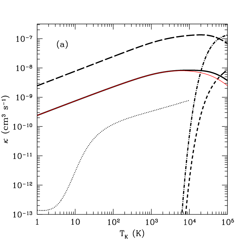
Figure 2: (a): Rate coefficients. The thick solid line shows $\kappa_{10}$, the spin de-excitation rate from elastic collisions below the $n=2$ threshold. The thin solid line shows the same quantity if we only include the $L=0$ partial wave. The long-dashed and dot-dashed curves show $\kappa_{n<2}$ and $\kappa_{n\geq 2}$, respectively. The short-dashed curve shows $\kappa_{2p}$. For comparison, the dotted curve shows $\kappa_{10}^{\rm HH}$. (b): The solid curve shows the ratio of the Liszt (2001) fit for $\kappa_{10}$ to the exact result. The dashed curve shows the ratio of the $L=0$ solution to the full result.

In practice, $\kappa_{10}$ quickly becomes irrelevant once the $n=2$ excitation threshold is reached, because the Ly$\alpha$ background generated by collisional excitations and subsequent radiative de-excitations will then dominate the spin de-excitation process. The production rate of Ly$\alpha$ photons (in units of photons per volume per second) is $\epsilon_{\alpha}=n_{\rm HI}n_{e}\kappa_{\alpha}$, where $\kappa_{\alpha}$ is the rate coefficient for excitations that eventually produce Ly$\alpha$ photons and $n_{\rm HI}$ is the density of hydrogen atoms. For a simple estimate, we set $\kappa_{\alpha}=\kappa_{2p}$, the rate of direct excitations to the $2p$ level. This is a lower limit because of cascades from higher levels: note that although roughly one-third of excitations to higher $p$ states produce Ly$\alpha$ photons (Hirata, 2006; Pritchard & Furlanetto, 2006b, a), the cross sections for these excitations are significantly smaller than the cross section for the $1s$–$2p$ transition, so the approximation is justified. (For example, $\kappa_{3s}$ is nearly fifty times smaller than $\kappa_{2p}$.) Under this approximation, the background flux at the Ly$\alpha$ resonance (assuming neutral helium) is

$$J_{\alpha}=\frac{c}{4\pi}x_{\rm HI}(1-x_{\rm HI})\frac{n_{H}^{2}(z)\kappa_{2p}}{\nu_{\alpha}H(z)},$$ (20)

where $\nu_{\alpha}$ is the frequency of the Ly$\alpha$ transition. In our cosmology, the coupling coefficient is then

$$x_{\alpha} \sim S_{\alpha}\left(\frac{\kappa_{2p}}{2.5\times 10^{-15}\mbox{ cm${}^{3}$ s${}^{-1}$}}\right)\left(\frac{1+z}{10}\right)^{7/2}$$ (21)

$$\times\left[\frac{x_{\rm HI}(1-x_{\rm HI})}{0.25}\right].$$

Using the cross sections calculated below, we find that $\kappa_{2p}$ is sufficiently large for Ly$\alpha$ scattering to dominate at $T_{K}\approx 6200\mbox{ K}$; see §3.3 for a more detailed discussion.

Overall, then, the effect of electronic excitations of hydrogen is to limit the applicability of the present calculations at high temperatures (above $T_{K}\approx 1.5\times 10^{4}\mbox{ K}$). Between that limit and $T_{K}\approx 6200\mbox{ K}$, the effects of Ly$\alpha$ photons must also be included.

3.2 The cross section

Having considered all the possible mechanisms for spin de-excitation, we have found that the spin-exchange mechanism does indeed dominate under astrophysical conditions, at least to the fraction of a percent level. There are possibly some effects of H^- resonances in the region around $k=0.8$ Ry, but otherwise our results are valid to better than the percent level up to $T_{K}\approx 1.5\times 10^{4}\mbox{ K}$.

In this section we proceed to calculate actual spin de-excitation cross sections from the spin exchange rates. Our inclusion of higher-order partial waves is the principal improvement over previous calculations. Field (1958) used the approximate $S$-wave phase shifts of Massey & Moiseiwitch (1951), which differ from the true values by several percent over this energy range. Most significantly, their scattering lengths differ by $\sim 25\%$ from the correct values. Smith (1966) used the (near-exact) $S$-wave phase shifts of Schwartz (1961) but did not include the $L>0$ terms.

Figure 1 shows $\sigma_{\rm se}$ as a function of collision energy. The solid curve includes the $L=0$–$3$ terms, while the dashed curve includes only $L=0$ and thus shows nearly the same cross section used by Smith (1966). Clearly the higher-order partial waves become important at $k\ga 0.1$, where non-zero angular momentum collisions become common. In fact, the $P$-wave makes up the vast majority of the difference (had we included only $L=0$ and $1$, the solid curve would appear the same except for the highest-energy resonance). Note the resonance structure at $k>0.8$; fortunately, although $\sigma_{\rm se}$ changes rapidly in this regime, the resonances constitute only a small part ($\Gamma\la 3\times 10^{-3}$ Ry) of the energy range.

3.3 The rate coefficient

The H–e^- collisional spin de-excitation rate coefficient is

$$\kappa_{10}=\sqrt{\frac{8k_{B}T_{K}}{\pi M}}\bar{\sigma}_{\rm se},$$ (22)

where the prefactor is the mean collision velocity, $M\approx m_{e}$ is the reduced mass of the H–e^- system, and the thermally-averaged cross section is

$$\bar{\sigma}_{\rm se}=\frac{1}{(k_{B}T_{K})^{2}}\int_{0}^{\infty}{\rm d}E\,\sigma_{\rm se}(E)Ee^{-E/k_{B}T_{K}}.$$ (23)

Similarly, we can define $\kappa_{n<2}$, the rate coefficient for all collisions below the $n=2$ threshold, with the replacement $\sigma_{\rm se}\rightarrow\sigma_{\rm tot}$.

The heavy solid line in Figure 2a shows $\kappa_{10}$ if we include only collisions below the $n=2$ threshold. (In other words, we truncate the integral in eq. 23 at 10.2 eV; this restriction causes the decline at $T_{K}\ga 40,000\mbox{ K}$.) At low temperatures, it is nearly proportional to $T_{K}^{1/2}$ (which comes from the velocity factor): scattering is dominated by electrons near zero energy, where the amplitude is essentially set by the scattering lengths $a_{s,t}$. $\kappa_{10}$ flattens out at higher temperatures because $\sigma_{\rm se}$ declines with energy (see Fig. 1). We note that the resonances in Figure 1 are so narrow that they never affect $\kappa_{10}$ by more than $1\%$. In contrast, the dashed curve shows the total rate $\kappa_{n<2}$ for all collisions below the $n=2$ threshold. Only $\sim 10\%$ of collisions actually result in a net change of hydrogen spin.

For comparison, the dotted curve in Figure 2a shows the corresponding de-excitation rate coefficient for H-H collisions. The data at $T_{K}\la 300\mbox{ K}$ are taken from Zygelman (2005). At higher temperatures, we use cross sections from K. Sigurdson (private communication, also tabulated in Furlanetto et al. 2006). We do not show $\kappa_{10}^{\rm HH}$ at $T_{K}>10^{4}\mbox{ K}$ because Sigurdson did not include excitation to $n\geq 2$ states from H–H collisions. At high temperatures, $\kappa_{10}/\kappa_{10}^{\rm HH}\sim\sqrt{m_{p}/m_{e}}$ (comparable to the relative velocities of the scattering species). The hydrogen cross section is much smaller at $T_{K}\la 100\mbox{ K}$ because of an accidental cancellation in the $S$-wave cross sections (Zygelman, 2005; Sigurdson & Furlanetto, 2006).

The thin solid curve shows the cross section if we include only the $L=0$ term (this is essentially identical to the result of Smith 1966); we also show the ratio between this version and our result by the dashed curve in Figure 2b. As expected, higher-order partial waves only affect $\kappa_{10}$ at $T_{K}\ga 1000\mbox{ K}$, where a substantial fraction of the electrons have large enough momenta for the $L=1$ term to become significant.

Calculations in the literature often use the fit to $\kappa_{10}$ proposed by Liszt (2001), which is based on the high-temperature results of Smith (1966). The solid line in Figure 2b compares this function to the exact value. At low temperatures, it exceeds our results by several percent, and it systematically underestimates $\kappa_{10}$ at $T\ga 3000\mbox{ K}$. We therefore recommend interpolating the exact rate coefficients; to this end, Table 1 presents our results in numerical form.

Table 1: Electron-hydrogen spin de-excitation rates

$T_{K}\,({\rm K})$	$\kappa_{10}\,(10^{-9}\,{\rm cm^{3}\ s^{-1}})$	$T_{K}\,({\rm K})$	$\kappa_{10}\,(10^{-9}\,{\rm cm^{3}\ s^{-1}})$
1	0.239	1000	5.92
2	0.337	2000	7.15
5	0.530	3000	7.71
10	0.746	5000	8.17
20	1.05	7000	8.32
50	1.63	10,000	8.37
100	2.26	15,000	8.29
200	3.11	20,000	8.11
500	4.59

Unfortunately, there are no accurate calculations of $\sigma_{\rm se}$ above the $n=2$ threshold; typically only the total cross sections for elastic scattering, excitation, and ionization are presented (from which the spin-exchange cross section – a coherent sum of the singlet and triplet scattering amplitudes – cannot readily be extracted). However, we can at least estimate the total rate (including elastic scattering, excitation, and ionization) for interactions above threshold (which we will call $\kappa_{n\geq 2}$); comparing that to $\kappa_{n<2}$ provides an estimate of the temperature at which our calculation breaks down. To compute $\sigma_{n\geq 2}$, we interpolate the cross sections given by Wang & Callaway (1994) for energies between the $n=2$ and $n=3$ thresholds (which include elastic collisions as well as excitations to the $2s$ and $2p$ levels) and the total cross sections for $E>13.6\mbox{ eV}$ from the Convergent Close Coupling online database (see Bray et al. 2002 and references therein), which includes elastic scattering, excitation to all levels through $4f$, and ionization.

The dot-dashed curve in the left panel of Figure 2 shows the resulting rate coefficient $\kappa_{n\geq 2}$. It increases rapidly at $T_{K}\ga 10^{4}\mbox{ K}$, when the tail of the electron velocity distribution begins to populate the $E>10.2\mbox{ eV}$ space. We find $\kappa_{n\geq 2}/\kappa_{n<2}\approx 0.01,\,0.1,$ and $1$ at $T_{K}\approx(1.5,\,2.3,\,6.0)\times 10^{4}\mbox{ K}$. As mentioned above, we therefore expect that our $\kappa_{10}$ is accurate to better than one percent at $T_{K}<1.5\times 10^{4}\mbox{ K}$.

The short-dashed curve in Figure 2a shows $\kappa_{2p}$ (computed in the same way as the total cross section), which we used in §3.1.5 above to calculate the temperature at which Ly$\alpha$ scattering becomes important; $\kappa_{2p}$ is typically several percent of $\kappa_{n\geq 2}$. Obviously it is an extremely steep function of temperature, so we show a closeup of the regime of interest in Figure 3. We find that $\kappa_{2p}$ reaches the level required by equation (21) at $T_{K}\approx 6200\mbox{ K}$. At $T_{K}\la 5000\mbox{ K}$, the Ly$\alpha$ background can be neglected in most applications; on the other hand, by $T_{K}\sim 8000\mbox{ K}$, it will entirely dominate. In detail, the total Ly$\alpha$ production rate will be slightly larger than shown here because of radiative cascades from higher levels (Pritchard & Furlanetto, 2006a). However, the extremely steep dependence of this rate coefficient on temperature suggests that in practice such minor corrections will not be very important. We also note again that Figure 3 assumes a thermal distribution of electrons; if a nonthermal population of fast electrons exists (as is the case if X-rays permeate the IGM; Chen & Miralda-Escude 2006; Chuzhoy et al. 2006), they can collisionally excite higher levels and so produce Ly$\alpha$ photons even if the mean IGM temperature is much smaller. Thus Ly$\alpha$ production is probably always somewhat important, but its details depend on the extremely uncertain radiation backgrounds (Sethi, 2005; Furlanetto, 2006). We will therefore not address this possibility here.

Figure 3: Rate coefficient for H–e^- collisional excitation to the $2p$ level.

4 Astrophysical applications

Although $\kappa_{10}$ is much larger than the corresponding quantity for H–H collisions, H–e^- collisions are often ignored in calculating the spin temperature of the 21 cm line in the high-redshift IGM. At the small residual ionized fractions ($\bar{x}_{i}\sim 2\times 10^{-4}$) expected following standard cosmological recombination (Seager et al., 1999), this is a reasonable assumption. However, once $\bar{x}_{i}\ga 0.01$, electron collisions become quite important (e.g., Nusser 2005; Kuhlen et al. 2006). In this section, we will apply our improved calculation of $\kappa_{10}$ to some simple cosmological examples. We will only consider the regime $T_{K}\la 3000\mbox{ K}$, where the effects of electronic excitations of hydrogen are much less than one percent and the Ly$\alpha$ background from collisional excitations can be ignored (assuming a Maxwell-Boltzmann electron distribution and hence neglecting any X-ray background). These examples are therefore not particularly realistic, but they isolate the major effects of electron collisions and so are useful model problems.

Figure 4: 21 cm brightness temperature fluctuations at $z=12$ for $T_{K}=10^{3}\mbox{ K}$. The thin curves take $\bar{x}_{i}=0,\,0.01,\,0.05,\,0.1$, and $0.2$, from bottom to top, with $x_{\alpha}=0$. The upper thick curve shows the fluctuation amplitude if $T_{S}=10^{3}\mbox{ K}$, while the lower thick curve shows the fluctuation amplitude if the temperature and ionization fraction are those expected in an adiabatically cooling Universe.

Equation (1) shows that perturbations in the density, temperature, ionized fraction, and velocity all source fluctuations in the brightness temperature. Because, to linear order in $k$-space, velocity perturbations are simply proportional to density perturbations, we can write the Fourier transform of the fractional 21 cm brightness temperature perturbation as (Furlanetto et al., 2006)

$$\tilde{\delta}_{21}({{\bf k}})=(\beta+\mu^{2})\tilde{\delta}+\beta_{x}\tilde{\delta}_{x}+\beta_{T}\tilde{\delta}_{T},$$ (24)

where $\tilde{\delta}$, $\tilde{\delta}_{x}$, and $\tilde{\delta}_{T}$ are the Fourier-space fractional perturbations in density, neutral fraction, and $T_{K}$, respectively, and $\mu$ is the cosine of the angle between the line of sight and the wavevector ${{\bf k}}$. The $\beta_{i}$ factors are linear expansion coefficients. For simplicity, we will assume that $\delta_{T}=0$ (see Pritchard & Furlanetto 2006a for a detailed discussion of temperature fluctuations). The relevant expansion coefficients $\beta_{i}$ are then (Furlanetto et al., 2006)

$$\beta = 1+\frac{1}{1+x_{c}},$$ (25)

$$\beta_{x} = 1+\frac{x_{c}^{\rm HH}-x_{c}^{\rm eH}}{x_{c}(1+x_{c})}.$$ (26)

We assume that $\delta_{x}$ is determined by photoionization equilibrium,

$$\delta_{x}=\left(\frac{1-\bar{x}_{\rm HI}}{1+\bar{x}_{\rm HI}}\right)\delta\equiv g_{x}\delta_{x},$$ (27)

where $\bar{x}_{\rm HI}$ is the global mean neutral fraction. This is not a particularly good assumption during reionization (again, see Pritchard & Furlanetto 2006a for a more careful treatment), but it allows us to compare our work with previous results (Nusser, 2005). In any case, $\delta_{x}$ generally makes only a small contribution to the fluctuations.

From equation (24), it then follows that the spherically-averaged power spectrum of 21 cm fluctuations can be written

$$P_{21}(k)=\bar{\delta T}_{b}^{2}(\beta^{\prime 2}+2\beta^{\prime}/3+1/5)P_{\delta\delta}(k),$$ (28)

where $\bar{\delta T}_{b}$ is the mean brightness temperature, $P_{\delta\delta}(k)$ is the matter power spectrum, and $\beta^{\prime}=\beta+\beta_{x}g_{x}$. We will quote our results in terms of the mean temperature fluctuation as a function of scale, $\Delta_{21}^{2}(k)=(k^{3}/2\pi^{2})P_{21}(k)$.

Figure 5: Ratio of the 21 cm brightness temperature fluctuation amplitude to its value in a purely neutral Universe, as a function of $\bar{x}_{i}$. The thin and thick curves are for $z=12$ and $z=20$, respectively. The solid and dashed lines take $T_{K}=100$ and $3000\mbox{ K}$. The dotted curve shows the fluctuations at $z=12$ and $T_{K}=3000\mbox{ K}$ when $\delta_{x}=0$.

Figure 4 shows the brightness temperature fluctuations in some example scenarios at $z=12$. The lower thick solid curve shows $\Delta_{21}$ for the standard calculation, in which the only heat source is Compton scattering of CMB photons (computed with RECFAST; Seager et al. 1999). In this case the gas is cold ($T_{K}=3.51\mbox{ K}$) and almost entirely neutral ($\bar{x}_{i}=1.8\times 10^{-4}$), so both collisional coupling and the 21 cm fluctuations are extremely weak. The upper thick solid curve shows a contrasting case in which $T_{S}=10^{3}\mbox{ K}$ and $\bar{x}_{i}=0$. Here the IGM has saturated in emission.

The thin curves assume $T_{K}=10^{3}\mbox{ K}$ and take $\bar{x}_{i}=0,\,0.01,\,0.05,\,0.1$, and $0.2$, from bottom to top. Naively, of course, one would expect $\Delta_{21}$ to decrease as $\bar{x}_{i}$ increases, simply because there is less neutral gas. But, as we have seen, H–e^- collisions are much more efficient at changing $T_{S}$ than H–H interactions, so they can enhance the fluctuation amplitude by more than a factor of two even at these relatively small amounts of ionization. As a result, warm gas can seed milliKelvin fluctuations even in the absence of a Ly$\alpha$ background (regardless of the heat source).

Figure 5 shows how the amplification factor depends on $\bar{x}_{i}$ by comparing to the fluctuation amplitude in fully neutral gas. First consider the two thick curves, which show the ratio between the signals with and without ionization at $z=20$. The solid and dashed curves assume $T_{K}=100$ and $3000\mbox{ K}$, respectively. The amplification is larger for cooler gas because the overall coupling is weaker at lower temperatures, and the addition of free electrons makes more of a difference. Interestingly, electron coupling provides a large enough boost that ionizing the gas continues to increase $\Delta_{21}$ until $\bar{x}_{i}$ is quite large – even as high as $90\%$ at the lower temperature.

The thin curves show the same ratios at $z=12$. Here the amplification is even larger because the densities are smaller (and hence the coupling weaker for a given $T_{K}$ and $\bar{x}_{i}$). For $T_{K}=100\mbox{ K}$, we also show the ratio assuming $\delta_{x}=0$ (rather than determined by photoionization equilibrium) with the dotted curve. Obviously, variations in the ionized fraction play only a minor role compared to the density fluctuations.

Our results can be compared directly with those of Nusser (2005), who presented more detailed calculations of 21 cm fluctuations in a warm Universe (in his case, one flooded with X-ray photons). He used the $\kappa_{10}$ values calculated by Field (1958), following the approximate phase shifts of Massey & Moiseiwitch (1951). These overestimated the scattering lengths by $\sim 25\%$, so our predicted amplitudes are somewhat smaller than his. Note again that, because we have neglected fast photoelectrons from X-rays (Chen & Miralda-Escude, 2006; Chuzhoy et al., 2006), as well as temperature fluctuations (Pritchard & Furlanetto, 2006a), these Figures are probably too simplistic to offer anything more than basic intuition.

5 Discussion

We have computed the spin de-excitation rates for hydrogen in the ground state during electron-hydrogen collisions. Previous calculations assumed that spin exchange through elastic $S$-wave scattering was the only relevant mechanism. Our analysis showed that while spin exchange does dominate spin de-excitation, higher partial waves contribute significantly to the total de-excitation rate. We used newer calculations of the elastic scattering phase shifts for the $L=0$–$3$ partial waves (Wang & Callaway, 1994) to re-compute $\kappa_{10}$. Our main results are presented in Table 1. They remain accurate up to $T_{K}\la 1.5\times 10^{4}\mbox{ K}$, where collisions above the $n=2$ threshold begin to become important at the percent level. Our results differ from Smith (1966) and especially from the widely-used fit in Liszt (2001) by several percent over the range $1\mbox{ K}<T_{K}<10^{4}\mbox{ K}$.

We have also shown that spin coupling produced directly through H–e^- collisions will become a secondary effect at $T_{K}\ga 6200\mbox{ K}$, because Ly$\alpha$ photons produced through collisional excitations easily dominate the spin coupling in this regime. Although the excitation rate to the $2p$ level (and to other levels that cascade through Ly$\alpha$) can be much smaller than the collisional spin de-excitation rate, each Ly$\alpha$ photon scatters $\sim 10^{5}$ times before redshifting out of resonance. This dramatically boosts the efficiency of the radiation background relative to collisions. In practice, the Ly$\alpha$ background may be important at even lower temperatures. In our calculations, we have assumed a Maxwell-Boltzmann distribution of electron velocities, but even a small population of nonthermal high-energy electrons can induce significant Ly$\alpha$ coupling. For example, X-rays produce fast secondary electrons able to excite hydrogen collisionally, which can easily produce such a background (Chen & Miralda-Escude, 2006; Chuzhoy et al., 2006).

We also considered some simple applications of our results to the high-redshift IGM. Electron-hydrogen collisions are likely to be most important if the radiation background is dominated by X-rays, so that the IGM becomes warm and weakly ionized. Such scenarios are particularly common when black hole accretion provides a significant fraction of the ionizing flux (Ricotti & Ostriker, 2004; Ricotti et al., 2005; Kuhlen et al., 2006). We have seen that the typical 21 cm fluctuation amplitude can reach the milliKelvin level even without a significant ultraviolet background. Our rate coefficients will be useful in assessing the implications of such scenarios for the 21 cm sky.

SRF thanks the Tapir group at Caltech for their hospitality while much of this work was completed. This publication has been approved for release as LA-UR-06-5395. Los Alamos National Laboratory, an affirmative action/equal opportunity employer, is operated by Los Alamos National Security, LLC, for the National Nuclear Security Administration of the U.S. under contract DE-AC52-06NA25396.

References

- Allison & Dalgarno (1969) Allison A. C., Dalgarno A., 1969, ApJ, 158, 423
- Barkana & Loeb (2005) Barkana R., Loeb A., 2005, ApJ, 624, L65
- Berestetskii et al. (1982) Berestetskii V. B., Lifshitz E. M., Pitaevskii V. B., 1982, Quantum Electrodynamics, 2nd ed.. Oxford, UK: Elsevier
- Bethe & Bacher (1936) Bethe H. A., Bacher R. F., 1936, Reviews of Modern Physics, 8, 82
- Bharadwaj & Ali (2004) Bharadwaj S., Ali S. S., 2004, MNRAS, 352, 142
- Bray et al. (2002) Bray I., Fursa D. V., Kheifets A. S., Stelbovics A. T., 2002, Journal of Physics B Atomic Molecular Physics, 35, 117
- Burke & Schey (1962a) Burke P. G., Schey H. M., 1962a, Physical Review, 126, 147
- Burke & Schey (1962b) Burke P. G., Schey H. M., 1962b, Physical Review, 126, 163
- Callaway (1978) Callaway J., 1978, Physics Letters A, 65, 199
- Chen & Kamionkowski (2004) Chen X., Kamionkowski M., 2004, PRD, 70, 043502
- Chen & Miralda-Escudé (2004) Chen X., Miralda-Escudé J., 2004, ApJ, 602, 1
- Chen & Miralda-Escude (2006) Chen X., Miralda-Escude J., 2006, submitted to ApJ (astro-ph/0605439)
- Chuzhoy et al. (2006) Chuzhoy L., Alvarez M. A., Shapiro P. R., 2006, submitted to ApJ (astro-ph/0605511)
- Chuzhoy & Shapiro (2005) Chuzhoy L., Shapiro P. R., 2005, submitted to ApJ (astro-ph/0512206)
- Condon & Shortley (1963) Condon E. U., Shortley G. H., 1963, The theory of atomic spectra. Cambridge, UK: Cambridge University Press
- Das & Rudge (1976) Das J. N., Rudge M. R. H., 1976, Journal of Physics B Atomic Molecular Physics, 9, L131
- Eisenstein & Hu (1998) Eisenstein D. J., Hu W., 1998, ApJ, 496, 605
- Field (1958) Field G. B., 1958, Proc. I.R.E., 46, 240
- Field (1959) Field G. B., 1959, ApJ, 129, 536
- Fletcher et al. (1985) Fletcher G. D., Alguard M. J., Gay T. J., Hughes V. W., Wainwright P. F., Lubell M. S., Raith W., 1985, PRA, 31, 2854
- Furlanetto (2006) Furlanetto S., 2006, in press at MNRAS (astro-ph/0604040)
- Furlanetto & Pritchard (2006) Furlanetto S., Pritchard J. R., 2006, submitted to MNRAS (astro-ph/0605680)
- Furlanetto et al. (2006) Furlanetto S. R., Oh S. P., Briggs F. H., 2006, Physics Reports, in press (astro-ph/0608032)
- Furlanetto et al. (2006) Furlanetto S. R., Pierpaoli E., Oh S. P., 2006, in preparation
- Furlanetto et al. (2004) Furlanetto S. R., Zaldarriaga M., Hernquist L., 2004, ApJ, 613, 1
- Gol’dman & Krivchenkov (1993) Gol’dman I. I., Krivchenkov V. D., 1993, Problems in Quantum Mechanics. New York: Dover Publications
- Hirata (2006) Hirata C. M., 2006, MNRAS, 367, 259
- Hirata & Sigurdson (2006) Hirata C. M., Sigurdson K., 2006, submitted to MNRAS (astro-ph/0605071)
- Iliev et al. (2003) Iliev I. T., Scannapieco E., Martel H., Shapiro P. R., 2003, MNRAS, 341, 81
- Jackson (1999) Jackson J. D., 1999, Classical Electrodynamics, 3rd ed.. New York: John Wiley & Sons
- Kuhlen & Madau (2005) Kuhlen M., Madau P., 2005, MNRAS, 363, 1069
- Kuhlen et al. (2006) Kuhlen M., Madau P., Montgomery R., 2006, ApJ, 637, L1
- Liszt (2001) Liszt H., 2001, A&A, 371, 698
- Loeb & Zaldarriaga (2004) Loeb A., Zaldarriaga M., 2004, Physical Review Letters, 92, 211301
- Madau et al. (1997) Madau P., Meiksin A., Rees M. J., 1997, ApJ, 475, 429
- Massey & Moiseiwitch (1951) Massey H. S. W., Moiseiwitch B. L., 1951, Proc. Roy. Soc. A, 205, 483
- Mott & Massey (1965) Mott N. F., Massey H. S. W., 1965, The Theory of Atomic collisions. Clarendon Press: Oxford, U.K.
- Naoz & Barkana (2005) Naoz S., Barkana R., 2005, MNRAS, 362, 1047
- Nusser (2005) Nusser A., 2005, MNRAS, 359, 183
- Oh (2001) Oh S. P., 2001, ApJ, 553, 499
- Pierpaoli (2004) Pierpaoli E., 2004, Physical Review Letters, 92, 031301
- Poet (1978) Poet R., 1978, J. Physics B, 11, 3081
- Pritchard & Furlanetto (2006a) Pritchard J. R., Furlanetto S. R., 2006a, submitted to MNRAS (astro-ph/0607234)
- Pritchard & Furlanetto (2006b) Pritchard J. R., Furlanetto S. R., 2006b, MNRAS, 367, 1057
- Purcell & Field (1956) Purcell E. M., Field G. B., 1956, ApJ, 124, 542
- Register & Poe (1975) Register D., Poe R. T., 1975, Physics Letters A, 51, 431
- Ricotti & Ostriker (2004) Ricotti M., Ostriker J. P., 2004, MNRAS, 352, 547
- Ricotti et al. (2005) Ricotti M., Ostriker J. P., Gnedin N. Y., 2005, MNRAS, 357, 207
- Schwartz (1961) Schwartz C., 1961, Physical Review, 124, 1468
- Scott & Rees (1990) Scott D., Rees M. J., 1990, MNRAS, 247, 510
- Seager et al. (1999) Seager S., Sasselov D. D., Scott D., 1999, ApJ, 523, L1
- Seaton (1957) Seaton M. J., 1957, Proc. Roy. Soc. A, 241, 522
- Sethi (2005) Sethi S. K., 2005, MNRAS, 363, 818
- Shchekinov & Vasiliev (2006) Shchekinov Y. A., Vasiliev E. O., 2006, submitted to MNRAS (astro-ph/0604231)
- Shertzer & Botero (1994) Shertzer J., Botero J., 1994, PRA, 49, 3673
- Shimamura (1971) Shimamura I., 1971, J. Phys. Soc. Jpn., 30, 1702
- Sigurdson & Furlanetto (2006) Sigurdson K., Furlanetto S. R., 2006, in press at PRL (astro-ph/0505173)
- Smith (1966) Smith F. J., 1966, Plan. Space Sci., 14, 929
- Spergel et al. (2006) Spergel D. N., et al., 2006, submitted to ApJ (astro-ph/0603449)
- Temkin (1962) Temkin A., 1962, Physical Review, 126, 130
- Venkatesan et al. (2001) Venkatesan A., Giroux M. L., Shull J. M., 2001, ApJ, 563, 1
- Wang & Callaway (1993) Wang Y. D., Callaway J., 1993, PRA, 48, 2058
- Wang & Callaway (1994) Wang Y. D., Callaway J., 1994, PRA, 50, 2327
- Wouthuysen (1952) Wouthuysen S. A., 1952, AJ, 57, 31
- Zygelman (2005) Zygelman B., 2005, ApJ, 622, 1356