Galaxy bimodality versus stellar mass and environment

Abstract

We analyse a $z<0.1$ galaxy sample from the Sloan Digital Sky Survey focusing on the variation of the galaxy colour bimodality with stellar mass ${\cal M}$ and projected neighbour density $\Sigma$, and on measurements of the galaxy stellar mass functions. The characteristic mass increases with environmental density from about $10^{10.6}{\cal M}_{\odot}$ to $10^{10.9}{\cal M}_{\odot}$ (Kroupa IMF, $H_{0}=70$) for $\Sigma$ in the range 0.1–$10\,{\rm Mpc}^{-2}$. The galaxy population naturally divides into a red and blue sequence with the locus of the sequences in colour-mass and colour-concentration index not varying strongly with environment. The fraction of galaxies on the red sequence is determined in bins of 0.2 in $\log\Sigma$ and $\log{\cal M}$ ($12\times 13$ bins). The red fraction $f_{r}$ generally increases continuously in both $\Sigma$ and ${\cal M}$ such that there is a unified relation: $f_{r}=F(\Sigma,{\cal M})$. Two simple functions are proposed which provide good fits to the data. These data are compared with analogous quantities in semi-analytical models based on the Millennium $N$-body simulation: the Bower et al. (2006) and Croton et al. (2006) models that incorporate AGN feedback. Both models predict a strong dependence of the red fraction on stellar mass and environment that is qualitatively similar to the observations. However, a quantitative comparison shows that the Bower et al. model is a significantly better match; this appears to be due to the different treatment of feedback in central galaxies.

1 Introduction

Galaxies when characterised by their morphology or radial profiles, integrated or central colours, and total luminosity or stellar mass, exhibit a range of relationships. These include colour-morphology relations (Holmberg, 1958; Roberts & Haynes, 1994), and colour-magnitude relations separately for early-type galaxies (Faber, 1973) and late-type galaxies (Chester & Roberts, 1964). While it was often considered that the natural dividing line was between spirals and ellipticals/lenticulars (e.g. Tully, Mould & Aaronson 1982), it was not until the multi-wavelength Sloan Digital Sky Survey (SDSS) that the galaxy population was considered strongly bimodal in colour (Strateva et al., 2001). Even when considering other galaxy properties such as radial profiles, the natural division is into two galaxy populations (Hogg et al., 2002; Ellis et al., 2005; Ball et al., 2006). Given that large automated imaging surveys are better at defining a galaxy’s colour than morphology, it is more natural to describe a galaxy as being on the “red sequence” or “blue sequence” rather than being an “early type” or “late type”. This interpretation also has the advantage that galaxy colours are directly related to the star formation, dust and metal enrichment history of the galaxy and can thus be more readily interpreted in theoretical models.

A key goal of galaxy evolution theory is to explain the bimodality and the relationships within each sequence, and there has been considerable work in this area recently (e.g. Kang et al. 2005; Menci et al. 2005, 2006; Springel et al. 2005b; Avila-Reese 2006; Bower et al. 2006; Cattaneo et al. 2006; Croton et al. 2006; Dekel & Birnboim 2006; Perez et al. 2006). The key ingredient of many of these models is the inclusion of feedback from active galactic nuclei (AGN). Although AGN feedback (or its equivalent) is implemented in different ways in each of these models, the overall effect is to suppress cooling in massive halos. For example, in Bower et al. (2006) the AGN feedback suppresses quasi-hydrostatic cooling flows, while Croton et al. (2006) adopt a semi-empirical description for the AGN power related to the Bondi accretion rate. Bimodality of galaxy colours does not directly result from these schemes, however, the AGN feedback allows the star formation rate parameterisation to be adjusted in such a way as to simultaneously obtain a good description of the colour distribution at faint magnitudes and a good match to the shape of the luminosity function. In these models red galaxies at faint magnitudes are predominantly satellite galaxies of brighter systems, while at bright magnitudes the central galaxies are also red because of the AGN feedback (e.g. fig. 3 of Bower et al.). In the real universe, however, the association between galaxy colours and their location in the halo is unlikely to be so simple (Weinmann et al., 2006), and measurements of the dependence of galaxy colours on luminosity and redshift are an important constraint on the new generation of galaxy formation models. Analysis of the relationship between galaxy colours and environment will place important constraints on the processes defining galaxy evolution.

This paper provides a detailed analysis of the variation of the bimodality with stellar mass and environment. The plan of the paper is as follows: in § 1.1, we review a series of papers providing the buildup to this paper; in § 2, we describe the data; in § 3, we present the results; in § 4, we discuss the implications and compare the data with models; and in § 5, we summarise the main results. Fits to the mass functions are presented in the Appendix. The data represented in this paper is available at http://www.astro.livjm.ac.uk/$\sim$ikb/research/ or upon request.

1.1 Previous work

Baldry et al. (2004a, hereafter Paper I) characterised the volume-averaged colour-magnitude distribution of galaxies by fitting double Gaussian functions to the colour histograms in magnitude bins. This showed that the red sequence transitioned from a broader colour distribution at $M_{r}\sim-19$ to a narrow distribution for massive early types at $M_{r}\sim-21$ while the blue sequence become significantly redder over the range $-20$ to $-22$ (using centrally-weighted colours). This supported the suggestion of a transition in galaxy properties around $10^{10.5}\,{\cal M}_{\odot}$ (Kauffmann et al., 2003b) and the former is consistent with faint red-sequence galaxies forming more recently (De Lucia et al., 2004; Kodama et al., 2004) but not necessarily in the richest clusters (Andreon, 2006). The difference in star formation history for galaxies below and above the transition mass may be related to the balance between hydrostatic versus rapid cooling (Birnboim & Dekel, 2003; Kereš et al., 2005; Bower et al., 2006; Croton et al., 2006), or to the diversity of star formation histories of satellite galaxies at low masses (Bower, 1991).

Balogh et al. (2004a, hereafter Paper II) analysed H$\alpha$ emission strength as a function of galaxy environment. The H$\alpha$ equivalent width (EW) distribution is bimodal with the distribution of the star forming population (blue sequence) not depending strongly on environment. The fraction of galaxies with ${\rm EW}>4$Å varied continuously with environmental density and there was no evidence of a break density that had been reported before (Lewis et al., 2002; Gómez et al., 2003). This demonstrated the importance of describing the variation of the bimodal population by comparing the number of galaxies within each population rather than using a quantity averaged over both populations.

In Paper II, the results indicated a dependence of the star-forming fraction on scales of about 5 Mpc (after accounting for local environment). However, the interpretation is difficult because the small-scale measurement is noisy and the large-scale measurement could actually be adding information about the small-scale environment (Blanton et al., 2006), and Kauffmann et al. (2004) found no environmental dependence on scales larger than 1 Mpc. It is also known that for galaxies in clusters properties can depend on environment for scales smaller than 1 Mpc (Dressler, 1980; Whitmore & Gilmore, 1991). These argue for an $N$th nearest neighbour approach to measuring environmental density as the radius is smaller in high density regions and expands in low density regions where there are often insufficient galaxies on small scales (for a fixed luminosity cut).

Balogh et al. (2004b, hereafter Paper III) extended the double Gaussian fitting of Paper I to colour histograms across environment and luminosity. At fixed luminosity, the mean positions of the sequences become marginally redder with environmental density. For the red sequence, this can be explained by a small difference in age between low- and high-density environments of $\sim 2$ Gyr (Thomas et al., 2005) or less (Hogg et al., 2004; Bernardi et al., 2006). In contrast, the fraction of red-sequence galaxies varied strongly with environment as measured by projected density. No effect related to velocity dispersion of a group or cluster was detected which is consistent with the morphology-density relation being similar in groups and clusters (Postman & Geller, 1984).

Baldry et al. (2004b) confirmed the shifts in colour of the red and blue sequences, 0.05 and 0.1 in $u-r$, respectively, over a factor of 100 in projected density. The red fraction varied from 0% to 70% for low-luminosity galaxies and 50% to 90% for high-luminosity galaxies (see also Tanaka et al. 2004). The effects of environment and luminosity could be unified in that the fraction of red-sequence galaxies was related to a combined quantity: $\Sigma_{\rm mod}=(\Sigma/{\rm Mpc}^{-2})\,+\,(L_{r}/L_{r,{\rm norm}})\,$ where $\Sigma$ is the projected density and $L_{r,{\rm norm}}$ is luminosity of a galaxy with $M_{r}=-20.2$. In this paper, this effect is explored in more detail using a larger sample and by converting luminosity to stellar mass.

2 Data

In this section, the selection of data from the SDSS catalogue and the derived quantities for each galaxy are described. The basics of the SDSS are described in § 2.1 while the sample selection is described in § 2.2. The primary sample consists of spectroscopically observed galaxies but a larger sample was used to determine spectroscopic completeness (§ 2.3) and to measure uncertainties in environmental densities (§ 2.6) for which photometric redshifts were determined (§ 2.4). Number density corrections are described in § 2.7. The derived quantities include absolute magnitude $M_{r}$, rest-frame colour $C_{ur}$, inverse concentration index ${\cal C}$ (§ 2.5), projected density of neighbouring galaxies $\Sigma$ (§ 2.6), and an approximate stellar mass ${\cal M}$ (§ 2.8).

2.1 Sloan Digital Sky Survey

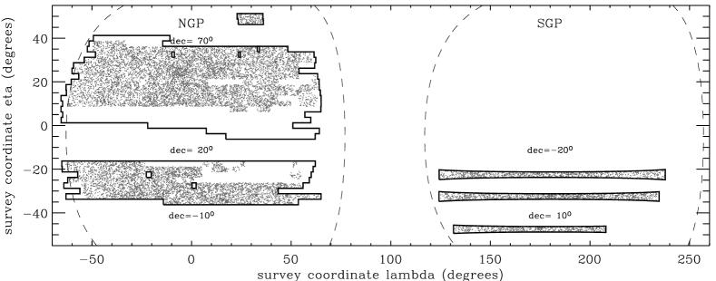
Figure 1: Sky coverage for SDSS DR4. The solid lines outline the primary photometric area, the dashed lines outline the galactic poles at 20° latitude, and the points show the positions for 4% of the galaxies that have been observed spectroscopically. The edges are are easier to define in SDSS survey coordinates, which is a spherical coordinate system [(eta,lambda)=(0,0) corresponds to (ra,dec)=(185,32.5)]. The photometric area covers 6670 deg² and the spectroscopic area covers 4780 deg² (Adelman-McCarthy et al., 2006).

The SDSS is a project, with a dedicated 2.5-m telescope, designed to image $10^{4}$ deg² and obtain spectra of $10^{6}$ objects (York et al., 2000; Stoughton et al., 2002). The imaging covers five broadbands, $ugriz$ with effective wavelengths of 355, 467, 616, 747 and 892 nm, using a mosaic CCD camera (Gunn et al., 1998). Spectra are obtained using a 640-fibre fed spectrograph with a wavelength range of 380 to 920 nm and a resolution of $\lambda/\Delta\lambda\sim 1800$.

The images are reduced using a pipeline photo that measures the observing conditions, and detects and measures objects. In particular, photo produces various types of magnitude measurement including: (i) ‘Petrosian’, the summed flux in an aperture that depends on the surface-brightness profile of the object; (ii) ‘model’, a fit to the flux using the best fit of a de-Vaucouleurs and an exponential profile; (iii) ‘PSF’, a fit using the local point-spread function. The magnitudes are extinction-corrected using the dust maps of Schlegel, Finkbeiner & Davis (1998). Details of the imaging pipelines are given by Stoughton et al. (2002).

Once a sufficiently large area of sky has been imaged, the data are analysed using ‘targeting’ software routines that determine the objects to be observed spectroscopically. The main sets of targets are: (i) the main galaxy sample (MGS), an $r<17.77$ selection (Strauss et al., 2002); (ii) luminous red galaxies (LRGs), an $r<19.5$ and colour-selected galaxy sample (Eisenstein et al., 2001); and (iii) quasi-stellar objects (QSOs; Richards et al. 2002). The targets from all the samples are then assigned to plates, each with 640 fibres, using a tiling algorithm (Blanton et al., 2003a). The main restriction is that two fibres cannot be placed within $55^{\prime\prime}$ on the same plate.

Spectra are taken using, typically, three 15-minute exposures in moderate conditions (the best conditions are used for imaging). The signal-to-noise ratio (S/N) is typically 10 per pixel ($\approx 1$–2Å) for galaxies in the MGS. The pipeline spec2d extracts, and flux and wavelength calibrates, the spectra. The spectra are then analysed by another pipeline that classifies and determines the redshift of the object. The redshift success is about 99% for galaxies considered in this paper.

2.2 Sample selection

The data used in this paper are from the SDSS Data Release Four (DR4) (Adelman-McCarthy et al., 2006). The primary sample consists of 151 642 galaxies with $r<17.77$ in the redshift range 0.010–0.085 (Sample C), with environmental densities determined from the distance to the 4th and 5th nearest neighbours with $M_{r}<-20$. However, the spectroscopic sample is not 100% complete; some galaxies are missed because of fiber-placement restrictions or are not yet observed, and there are edges to the sky coverage. Figure 1 shows the sky coverage for the photometric and spectroscopic data. In order to accurately account for missed spectra and to calculate completeness corrections, a larger photometric sample was considered. The galaxy sample selection and calculation of environmental densities are outlined below.

Objects were selected from the ‘CasJobs’ catalogue archive server with criteria $10.0<r<18.0\>,$ where $r$ is the Petrosian magnitude corrected for Milky-Way extinction, and $r_{\rm PSF}-r_{\rm model}>0.25\>.$ Photometric data (‘Galaxy’ table) and spectroscopic data (‘SpecObjAll’ table) where available were extracted. This produced an initial sample of 1 016 565 objects after removing duplicates (Sample A).

The next stage was to remove low-surface brightness artifacts and stars. A modified surface brightness was defined: $\mu_{\rm mod}=\mu_{r,{\rm 50}}-0.3(r-18)$ where $\mu_{r,{\rm 50}}$ is the mean surface brightness (SB) within the Petrosian half-light radius (eq. 5 of Strauss et al. 2002). The slope of 0.3 per magnitude was determined empirically from the SB-magnitude distribution so that the modified quantity was a better separator for stars, galaxies and artifacts. Figure 2 shows SB versus magnitude for various samples and the dividing lines. Objects with no spectroscopy were then trimmed to $18.5<\mu_{\rm mod}<24.0$ and ‘not saturated’ while spectroscopic objects were selected with $0.005<z<0.3.$ The trimmed sample contained 850 906 galaxies (Sample B).

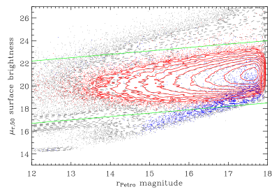
Figure 2: Surface brightness versus magnitude. The grey points and dashed contours represent all objects in Sample A; the red points and contours represent spectroscopically confirmed galaxies; and the blue points and contours represent stellar systems. The green lines show the limits imposed for photometric objects selected for Sample B. Note that most stars are rejected by the ‘not saturated’ criteria rather than the lower limit shown here.

2.3 Spectroscopic completeness

Spectroscopic completeness was determined from a related sample that included all spectra and was reduced to spectroscopic regions (634 395 galaxies, 478 385 with $r<17.77$). Galaxies were divided into classes based on their magnitude and the number of $r<17.77$ neighbours within $55^{\prime\prime}$ (0, 1 or $\geq 2$). The completeness was given by the number with spectra divided by the total number in a class. Figure 3 shows completeness versus magnitude. As expected the completeness is low above 17.77 and it becomes colour dependent (LRG selection). Thus, the final sample (Sample C) is restricted to this MGS limit where the completeness corrections are reliable. It is also clear that in order to determine the relative numbers of galaxies in different environments, it is important to account for the change in completeness as a function of the number of neighbours.

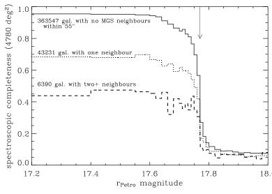
Figure 3: Spectroscopic completeness versus magnitude. The three lines represent galaxies with 0, 1 or $\geq 2$ neighbours within $55^{\prime\prime}$ (corresponding to the ‘fibre collision’ radius). The arrow shows the limit for MGS selection; the completeness drops prior to that because of changes in catalogue photometry and targeting algorithms. Here we have used the DR4 best photometry.

2.4 Photometric redshifts

Photometric redshifts were determined for Sample B using $\chi^{2}$ fitting to ‘training set’ galaxies with spectroscopic redshifts. The training set consisted of 396 302 galaxies out of a possible 410 206, with some galaxies rejected because of low redshift confidence, or extreme colours or colour errors. The data fitted for each galaxy were $r_{\rm Petro}$ and 4 ‘model’ colours: $u-g$, $g-r$, $r-i$, $i-z$. Thus, the underlying assumption is that the redshift-magnitude-colour distribution is similar for the galaxies with missing spectra as for the training set. Softening errors were added in quadrature, prior to determination of the $\chi^{2}$ values. These were 0.1 for the magnitude (larger for $r<13$) and 0.02 for the colours. The photometric redshift is then given by the weighted mean of training-set redshifts that fitted within $\chi^{2}<15$ (99% limit for 5 degrees of freedom). The weight for each match is given by $\exp({-\chi_{i}^{2}/2})\,w(z_{i})$, where $w(z_{i})$ is a minor adjustment to reduce the implicit weight given to redshift peaks within the training set. Objects with no matches within the limit or with few matches in the range $10<\chi^{2}<15$ were assumed to be outside the redshift range of the training set (i.e. stars, or $z>0.3$) and not considered in further analysis (13 741 objects). An initial photometric redshift error was determined from the standard deviation (with weights). These errors were then multiplied by a factor to give 95% confidence-limit errors:

$$z_{\rm err,95}=f_{95}\left(\frac{|z_{\rm photo}-z_{\rm spec}|}{z_{\rm err,initial}}\right)z_{\rm err,initial}$$ (1)

where $f_{95}()$ is the 95-th percentile of the expression determined for galaxies with spectroscopic redshifts. After calibration, the median value of $z_{\rm err,95}$ is 0.04 with typical values from 0.02 to 0.07. A minimum error of 0.02 was used in subsequent analysis.

2.5 Absolute magnitude, rest-frame colour and concentration index

The $r$-band absolute magnitude used in this paper is given by

$$M_{r}=r-k_{r}-5\log(D_{L}/{\rm\,10\,pc})$$ (2)

where: $r$ is the Milky-Way-extinction-corrected Petrosian magnitude; $D_{L}$ is the luminosity distance for a cosmology with $(\Omega_{m},\Omega_{\Lambda})_{0}$ = (0.3,0.7) and $H_{0}={\rm\,70\,km\,s^{-1}\,Mpc^{-1}}$, and; $k_{r}$ is the k-correction using the method of Blanton et al. (2003b); and rest-frame colour considered is given by

$$C_{ur}=(u_{\rm model}-k_{u})-(r_{\rm model}-k_{r})\>.$$ (3)

This was chosen as the optimum bimodality divider (Paper I). In effect, ‘model’ colours are centrally-weighted colours; the profile used is the best fit defined in the $r$-band light.

Galaxies with photometric redshifts have a range of uncertainty in their absolute magnitude. For calculation of environmental densities, their $k$-corrections were approximated by $k_{r}=[0.3+0.3(u-r)_{\rm model}]z_{\rm test}$ where $z_{\rm test}$ takes different values: the spectroscopic redshifts of the galaxies for which environmental density is measured.

The (inverse) concentration index was used in some of our analysis. The is given by ${\cal C}=R50/R90$ where $R50$ and $R90$ are the radii containing 50% and 90% of the Petrosian flux, averaged for the $r$ and $i$ bands. For typical galaxies, ${\cal C}$ ranges from 0.3 (concentrated) to 0.55; for comparison, a uniform disk would have ${\cal C}=0.75$.

2.6 Environmental densities

Densities were determined for Sample C using the information from Sample B. For environmental densities around each galaxy, we determine

$$\Sigma_{N}=\frac{N}{\pi d_{N}^{2}}$$ (4)

where $d_{N}$ is the projected comoving distance to the $N$th nearest neighbour that is a member of the density defining population (DDP) and that is within the allowed redshift range. The redshift range is $\pm\Delta zc=1000{\rm\,km/s}$ for neighbouring galaxies with spectroscopic redshifts and $\pm z_{err,95}$ for those with photometric redshifts only. The DDP are galaxies with $M_{r}<M_{r,{\rm limit}}-Q(z-z_{0})$ where $M_{r,{\rm limit}}=-20$, $Q=1.6$ is the evolution determined by Blanton et al. (2003c) and $z_{0}=0.05$. For galaxies with photometric redshifts only, $M_{r}$ was determined as if the galaxy were at the redshift of the galaxy whose environment was being measured. If the distance to the photometric edge $d_{\rm edge}$ were less than $d_{N}$ then $\pi d_{N}^{2}$ in Eq. 4 was replaced by the area within a chord crossing the circle, i.e., assuming the edge was straight.

The best estimate $\Sigma$ was obtained by averaging $\log\Sigma_{N}$ for $N=4$ and 5, and by averaging the calculation with spectro-$z$ only and the full sample B. In addition $\Sigma_{\rm min}$ was determined using $d_{N}$ with spectro-$z$ only, and $\Sigma_{\rm max}$ using the smaller of $d_{N}$ with Sample B and $d_{\rm edge}$. The uncertainty in $\log\Sigma$ was given by the larger of $\log\Sigma_{\rm max}-\log\Sigma$ and $\log\Sigma-\log\Sigma_{\rm min}$. For various environmental analyses, galaxies were only included if the uncertainty were less than 0.4 dex or less than 1 bin for galaxies in the minimum or maximum density bins. This more complicated procedure than simply using spectro-$z$ only and discarding galaxies near an edge ensures that the maximum number of galaxies can be used in any analysis; and it accurately accounts for ‘fibre collisions’.

Variations in the above parameters ($\Delta zc=1000{\rm\,km/s}$, $M_{r,{\rm limit}}=-20$, $N=4$ and 5) used to determine $\Sigma$ were tested. The results were not strongly dependent on the exact values, and the values chosen were near optimum and consistent with earlier papers (Paper II and Paper III). For typical galaxies, $\Sigma$ ranges from $0.05\,{\rm Mpc}^{-2}$ (void-like regions) to $20\,{\rm Mpc}^{-2}$ (clusters); for comparison, $\Sigma=0.5\,{\rm Mpc}^{-2}$ for the median environment around DDP galaxies whereas $\Sigma$ would be $0.14\,{\rm Mpc}^{-2}$ if DDP galaxies were distributed uniformly.

Figure 4 shows the number density of the DDP population versus redshift and the density of a more luminous $M_{r}<-21$ population. The near constant number density up to the completeness limit justifies the use of the evolution parameter determined by Blanton et al. (2003c). Sample C was restricted to the redshift range 0.010 to 0.085 for reliability of the environmental density measurements.

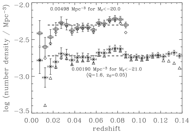
Figure 4: The number densities of galaxies versus redshift. The squares with error bars (including photometric redshifts) and diamonds (spectroscopic redshifts only) represent the number densities of galaxies more luminous than $-20$ (evolution corrected to $z=0.05$ with $Q=1.6$, Blanton et al. 2003c); this is the density defining population used in this paper. The crosses with error bars and triangles represent galaxies more luminous than $-21$. Above about $z>0.09$ and $z>0.13$, the counts become incomplete in the $r<18$ sample for the $M_{r}<-20$ and $M_{r}<-21$ populations, respectively. At $z<0.02$ there is incompleteness because of problems with automatic determination of photometric properties. Using $Q=1.6$ for the luminosity evolution, the number density evolution is near flat across the reliable redshift range, shown by the dashed lines.

2.7 Volume and density corrections

The DDP is volume limited but we also consider galaxies fainter than $M_{r}=-20$. For these and for some galaxies near $-20$, a volume correction is applied to the number density using a $V_{\rm max}$ method (Felten, 1976). Here, the weight of a galaxy for computing number densities is given by a factor $1/V_{\rm max}$ where $V_{\rm max}$ is the maximum volume over which the galaxy could be observed within the $r<17.77$ limit and the survey volume ($0.010<z<0.085$ over 1.52 steradians; $2.3\times 10^{7}{\rm\,Mpc}^{3}$).

The added complication when considering environment is the fact that the contribution of a particular environment bin to the volume-averaged number density can vary significantly as a function of redshift. To correct for this, we determine a relative volume ($f_{V}$) that a galaxy in a particular environment could be observed over the redshift range given by $V_{\rm max}$ ($0.010<z<z_{\rm max}$). This relative volume is a function of $z_{\rm max}$ and $\Sigma$ and can be determined by measuring the number densities of bright galaxies that can be viewed over the whole survey volume. The relative volume was determined in bins of 0.05 in $z$ and in $\Sigma$ (depending on the bins being used). In other words, $f_{V}$ is the number density of bright galaxies with $z<z_{\rm max}$ relative to the number density covering the whole redshift range (with reduced survey area to avoid edge effects). The number density of galaxies with a given $z_{\rm max}$ and $\Sigma$ was renormalised by $1/f_{V}$. This factor $f_{V}$ is in the range 0.6–1.1 for $z_{\rm max}\ga 0.03$ over 12 environment bins; $f_{V}$ is on average less than unity because galaxies are rejected when the uncertainty in $\Sigma$ is too large.

To summarise, there are three number density corrections for each galaxy in Sample C: (i) $1/C_{s}$ where $C_{s}$ is the spectroscopic completeness which is a function of $r$ and the number of MGS neighbouring galaxies within $55^{\prime\prime}$ (§ 2.3); (ii) $1/V_{\rm max}$ where $V_{\rm max}$ is a function of the absolute magnitude and the galaxy’s colours which determine $k$-corrections; (iii) $1/f_{V}$ where $f_{V}$ is the relative volume which is a function of $z_{\rm max}$ and $\Sigma$ when dividing the population into environment bins.

2.8 Conversion to stellar mass

The use of stellar mass as a galaxy variable has been widely promoted (e.g. Thronson & Greenhouse 1988; Prugniel & Simien 1996; Brinchmann & Ellis 2000; Benson et al. 2002; Bell et al. 2003; Pérez-González et al. 2003; Conselice et al. 2005; Gallazzi et al. 2005; Pannella et al. 2006). The total stellar mass of a galaxy is a more fundamental quantity than luminosity as has been shown by, for example, Kauffmann et al. (2003a). Galaxy stellar masses are typically derived by fitting stellar-population synthesis models to colours or spectra. However, there are systematic uncertainties that depend on the underlying set of allowed star-formation histories in the models as well as uncertainties in the models. Here, we use an approach similar to that of Bell & de Jong (2001) whereby we use a stellar mass-to-light ratio that is a function of one colour only. While uncertainties will remain, the method has the advantage of retaining a simple relation between the derived physical quantity, the selection function, and the rest-frame colour used in our analysis. Figure 5 shows a plot of stellar mass-to-light ratio versus $C_{ur}$ colour for $10^{4}$ galaxies analysed by the MPA Garching group and by K.G. The dashed line represents the relation that we use in our analysis.

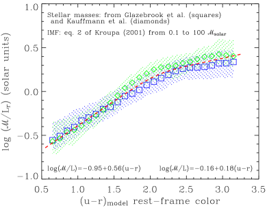
Figure 5: Correlation of galaxy stellar mass-to-light ratio with colour. Stellar masses were determined for a sample of $10^{4}$ galaxies. The blue squares and dotted-line region represent the median in 0.1 color bins and 1-sigma ranges computed by K.G. (Glazebrook et al., 2004). The green diamonds and region represent stellar masses computed by the MPA Garching group (Kauffmann et al., 2003a). The red dashed line represents a broken line fit to the data, with the coefficients shown in the plot.

3 Results

3.1 Colour-concentration relations as a function of stellar mass

In Paper I and Paper III, we divided the galaxy population by using double Gaussian fitting to the colour functions in luminosity bins. This separates the galaxy population into red and blue sequences. There was no consideration of the morphology or structure of the galaxies. This method is accurate if the colour functions are truly the sum of Gaussian distributions and if the errors are small. A more robust method of outlining the two sequences is to consider a joint distribution in colour and structure (Driver et al., 2006). Figure 6 shows the distribution of observed galaxies in colour versus concentration index for three different stellar mass ranges.

Figure 6: Colour versus concentration index for different stellar-mass ranges. The points and solid contours represent galaxies in our sample. The contours are logarithmically spaced in number density with 4 contours per factor of 10. The dashed lines show the position of possible colour or concentration-index dividers.

The peak of the red sequence gets redder (2.3 to 2.6) and more concentrated (0.38 to 0.32) with increasing mass ($\log{\cal M}$ from 9.5 to 11.0); while the blue sequence gets redder (1.5 to 2.1) with approximately the same concentration (0.45). This means that the natural dividing lines of the population are around ${\cal C}=0.4$ for all the stellar masses (vertical dashed lines in the figure) but the dividing line in colour gets redder (horizontal dashed lines). At lower masses, dividing using colour is significantly better than dividing using concentration index. At higher masses, while colour is still a reasonable divider, concentration index can be useful in robustly determining the colour mean and dispersion of each sequence.

In Paper I, a method for fitting double Gaussians to the colour functions is described. At each luminosity or mass bin, there are six parameters, amplitude, mean and dispersion for each sequence, given by $\phi_{\rm r},\mu_{\rm r},\sigma_{\rm r},\phi_{\rm b},\mu_{\rm b},\sigma_{\rm b}$. When the counts are low or the sequences are significantly merged together in colour (e.g. at the high-mass end), the solution is not well defined. With the robust method, $\mu_{\rm r}$ and $\sigma_{\rm r}$ are determined using galaxies with predominately high concentration (full weight for ${\cal C}<0.4$) while $\mu_{\rm b}$ and $\sigma_{\rm b}$ are determined using galaxies with low concentration (${\cal C}>0.4$). The amplitudes of each Gaussian are still determined using a fit to both populations but with the $\mu$ and $\sigma$ values fixed.

This method of determining the positions of the sequences is used in § 3.2, which then determines the best-fit dividing line in color, and in § 3.4. In § 3.5, only the dividing line is used.

3.2 Volume-averaged colour-magnitude and colour-mass relations

Figure 8 shows a comparison between colour-magnitude and colour-mass relations: $C_{ur}$ versus (a) $u$-band absolute magnitude, (b) $r$-band absolute magnitude, and (c) logarithm of the stellar mass. Note how the contours are almost vertical at the luminous end in Fig. 8(a) whereas the red sequence is dominant at the high mass end in Fig. 8(c).

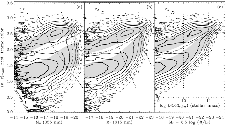
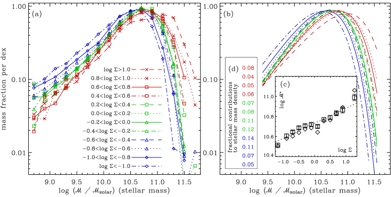
Figure 7: Comparison between galaxy colour-magnitude and colour-mass relations. Colour is plotted versus (a) $M_{u}$, (b) $M_{r}$ and (c) $\log{\cal M}$. The dashed and solid lines represent logarithmically-spaced density contours with 4 contours per factor of 10; the number densities are completeness and volume corrected. The dotted lines represent galaxies with stellar masses of $10^{10}$ and $10^{11}\,{\cal M}_{\odot}$. The grey regions represent the colour means and $\pm 1$-sigma ranges of the red and blue sequences. The dash-and-dotted lines represent the best-fit dividers between the sequences based on the criteria of Paper I.

Figure 8: Galaxy stellar mass functions. In panels (a) and (b), the symbols and lines represent different environments as shown in the legend of panel (a). Note the unusual $y$-axis, with respect to standard mass or luminosity functions, shows clearly that the ‘peak’ in the mass function is near the Schechter break ($\log{\cal M}^{*}$). Panel (a) shows the binned functions (the median errors are 5%) while panel (b) shows the Schechter function fits. Inset panel (c) shows $\log{\cal M}^{*}$ versus $\log\Sigma$. The diamonds represent $\log{\cal M}^{*}$ as defined by the parameter in the fit while the squares represent the peaks of the fits given by $\log[{\cal M}^{*}(\alpha+2)]\,$. Note that a standard Schechter function fit is only valid over the range from about 9.5 to 11.5, and there is a statistically significant upturn in the faint-end slope at low masses (cf. Paper I, Blanton et al. 2005b, Appendix). Inset panel (d) shows the approximate fractional contribution to the stellar mass density of the universe ($\Omega_{\rm stars}\approx 0.002$) for each environmental bin from high to low densities (top to bottom). Plots of the GSMFs using double Schechter fits and using number versus $\log{\cal M}$ are shown in Fig. 17.

In order to fit the mean positions of the sequences, we used a tanh plus a straight-line function as per Paper I. A general form of this ‘${\cal T}$ function’ is given by

$${\cal T}(x)=p_{0}+p_{1}x+q_{0}\tanh\left[\frac{x-q_{1}}{q_{2}}\right]$$ (5)

where $p_{0,1}$ are the straight line parameters; and $q_{0,1,2}$ are the tanh parameters. The fitting of the sequences followed the iteration outlined in § 4.2 of Paper I except with the addition of the robust method outlined in § 3.1 above for the double Gaussian fitting.

The grey regions in Fig. 8 show the mean position and dispersion along each sequence. A key point is that the blue sequence is significantly narrower versus stellar mass than luminosity, particularly near-UV luminosity (the color dispersion is about 0.23, 0.31, 0.37 for blue-sequence galaxies with $\log{\cal M}\sim 10.5$, $M_{r}\sim-21.0$, $M_{u}\sim-19.5$, respectively). This demonstrates that stellar mass is closer to a fundamental predictor of a galaxy’s colour than luminosity. The dash-and-dotted lines in the figure represent the best-fit dividing lines between the red and blue sequences using the optimal criteria of Paper I.

When dividing the galaxy population by environment, it becomes more difficult to proceed with the full fitting procedure. For cases where many environmental bins are used, the number of galaxies in each sequence is defined by galaxies redder and bluer than the best-fit dividing line [dash-and-dotted line in Fig. 8(c)]: $C_{ur,{\rm divide}}$ varies from 1.8 to 2.5 for $\log{\cal M}$ from 9.0 to 11.5; ${\cal T}$ function with parameters of $p_{0,1}=(2.18,0)$, $q_{0,1,2}=(0.38,10.26,0.85)$.

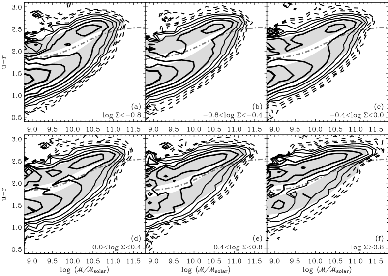
Figure 9: Colour versus stellar mass relations for different environments. Panel (a) represents void-like environments while panel (f) represents cluster-like environments. The dashed and solid lines represent logarithmically-spaced density contours. The grey regions outline the red and blue sequences. The dash-and-dotted lines show the best-fit divider from Fig. 8(c).

3.3 Environmental dependence of the galaxy stellar mass functions

Before considering the variation of the colour-mass relations it is important to note that the galaxy stellar mass functions (GSMFs) vary significantly with environment. The galaxy population was divided into 12 environment bins and 16 mass bins. Figure 8 shows the variation of the GSMFs with environment. The GSMFs are plotted using mass fraction normalised by total mass within each environment bin (i.e. the integral under each curve is unity). This has two advantages: (i) the $y$-axes values range over 2 orders of magnitude compared to about 4 when plotting number density; and (ii) the peak of each GSMF corresponds to the dominant contribution to the total stellar mass within an environment bin. This varies from $\log{\cal M}\sim 10.6$ to 11.0 from low to high densities; with the fractional contribution due to high mass galaxies ($\log{\cal M}\sim 11.5$) increasing by a factor of about 50.

The GSMFs can be characterised by fitting Schechter (1976) functions:

$$\phi_{N}\>\propto\>{\cal M}^{\alpha}e^{-{\cal M}/{\cal M}^{*}}$$ (6)

where $\phi_{N}\,{\rm d}{\cal M}$ is the number of galaxies with masses between ${\cal M}$ and ${\cal M}+{\rm d}{\cal M}$; or

$$\phi_{\log{\cal M}}\>\propto\>{\cal M}^{\alpha+2}e^{-{\cal M}/{\cal M}^{*}}$$ (7)

where $\phi_{\log{\cal M}}\,{\rm d}\log{\cal M}$ is the total mass of galaxies between $\log{\cal M}$ and $\log{\cal M}+{\rm d}\log{\cal M}$. Normalised $\phi_{\log{\cal M}}$ is plotted in Fig. 8. For a standard Schechter function, the peak of the $\phi_{\log{\cal M}}$ GSMF is given by ${\cal M}_{\rm peak}={\cal M}^{*}(\alpha+2)$. Thus, ${\cal M}_{\rm peak}$ can be considered an alternative characteristic mass for faint-end slopes around $-1$, which is less dependent on model choice (cf. Andreon 2004).

The Schechter fits are shown in Fig. 8(b) with $\log{\cal M}^{*}$ versus environment plotted in Fig. 8(c). A fit to $\log{\cal M}_{\rm peak}$ is shown by the dotted line, formally

$$\log[{\cal M}^{*}(\alpha+2)]=(10.73\pm 0.01)+(0.15\pm 0.01)\log\Sigma$$ (8)

The faint-end slope is approximately $-1$ over the fitted range which does not vary strongly with environment. A standard Schechter function does not fit the entire mass range. Fits to the extended mass range using a double Schechter function (Paper I) are shown in the Appendix.

The increase of the characteristic mass with local density of 0.4 dex, equivalent to 1 mag, is broadly consistent with other results. A precise quantitative comparison is difficult because of the different methods of determining environment and different wavelengths. Croton et al. (2005) found an increase of $\sim 1{\rm\,mag}$ between void and cluster-like environments using $b_{J}$ luminosities. Hoyle et al. (2005) found a difference of 0.9 mag between void and wall galaxies using $r$-band luminosity. There are many other analyses looking at luminosity functions versus group masses, cluster properties, etc. (e.g. Binggeli et al. 1988; Balogh et al. 2001; De Propris et al. 2003; Zandivarez et al. 2006). The main point is that the overall characteristic luminosity or mass increases with environmental density. This should be accounted for when comparing galaxy colours between different environments.

Figure 10: Colour versus concentration index across different environments for stellar masses around $10^{10}\,{\cal M}_{\odot}$. The points and solid contours represent galaxies in our sample. The dashed ellipses are fixed in each panel outlining the locus of the red- and blue-sequence galaxies. The dominant effect is clearly the increase in the fraction of galaxies on the red sequence with increasing density; while the locus of the sequences become marginally redder. The dash-and-dotted lines show the best-fit color divider for the mean mass.

3.4 Environmental dependence of the colour-mass and colour-concentration relations

The galaxy population was divided into environmental bins in order to determine the variation of the colour-mass relation. Figure 9 shows the colour-mass relations for six environmental bins ranging from $\log\Sigma<-0.8$ to $\log\Sigma>0.8$. The equivalent of the cluster red sequence is evident in Fig. 9(f); while the dominance of the blue sequence at lower masses is evident in Fig. 9(a-c) for the lower densities. While the red sequence is dominant at higher masses in all environments, the upper mass cutoff is increasing with environmental density. The best-fit dividing line from § 3.2 provides a reasonable color division between the two sequences in all environments as shown by the dash-and-dotted lines.

As noted in Paper III, the mean positions of the sequences as shown by the grey regions in Fig. 9 do not vary strongly with environment. This is also evident if one plots colour versus concentration index as a function of environment for different mass ranges. Figure 10 shows this for galaxies with masses around $10^{10}\,{\cal M}_{\odot}$. The clearly dominant effect is the increase in the fraction of galaxies on the red sequence as a function of environment.

3.5 Environmental and stellar mass dependence of the relative red- and blue-sequence numbers

In Baldry et al. (2004b), it was shown that the fraction of galaxies in the red sequence could be unified by a function of environmental density and luminosity. Here, we proceed with a similar analysis using stellar mass in place of luminosity. The population was divided into 12 environment bins and 13 mass bins. The fraction is defined as galaxies redder than the best-fit dividing line [Fig. 8(c) and 9]. Figure 11 shows the fraction of red-sequence galaxies (a) versus environment for different stellar masses and (b) versus stellar mass for different environments. Qualitatively the plots are similar: with increasing red fraction versus stellar mass or environment and a greater variation at the lower end of each scale.

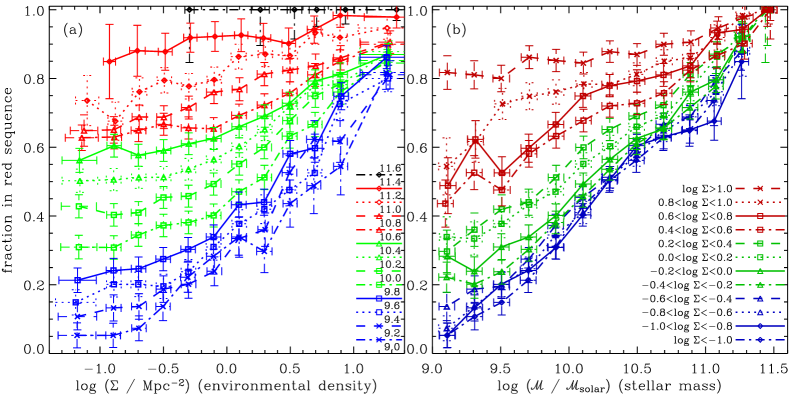
Figure 11: Fraction of red-sequence galaxies versus environment and versus stellar mass. In panel (a), the symbols and lines represent different stellar masses as shown in the legend ($\log{\cal M}$ from 9.0 to 11.6). In panel (b), the lines represent different environmental densities. Systematic errors of 0.03 were added in quadrature to the Poisson errors. Note the similarity between the two plots leads to the unification schemes shown in Fig. 12.

Both stellar mass and environment affect the probability of a galaxy being in the red sequence. First of all, we found an empirical relation that is based on the sum of projected environmental density and stellar mass:

$$f_{r}=0.5+a_{1}\log_{10}(\Sigma/a_{2}+{\cal M}/a_{3})$$ (9)

(with the constraint $0\leq f_{r}\leq 1$) where $f_{r}$ is the fraction of red-sequence galaxies and $a_{1,2,3}$ are the parameters to determine. Secondly, we found an empirical relation more naturally related to probability theory that is given by:

$$f_{r}=1-\exp\{-[(\Sigma/b_{1})^{b_{2}}+({\cal M}/b_{3})^{b_{4}}]\}$$ (10)

where $b_{1,2,3,4}$ are the parameters to determine. This function has the useful feature of asymptotically tending to 0 and 1 at the extremes. Figure 12 shows these empirical relations that were determined by minimising $\chi^{2}$. The values of the parameters are (a) 0.438, $10^{0.46}{\rm Mpc}^{-2}$, $10^{10.34}{\cal M}_{\odot}$ and (b) $10^{0.91}{\rm Mpc}^{-2}$, 0.69, $10^{10.72}{\cal M}_{\odot}$, 0.59. [Note an empirical law of the form $f_{r}=F(c\log\Sigma+\log{\cal M})$ does not work; the $\chi^{2}$ is about 200 higher for a quadratic function $F$.]

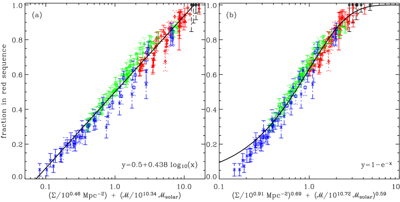
Figure 12: Fraction of red-sequence galaxies versus unified quantities: (a) using Eq. 9 and (b) using Eq. 10. The symbols and error bars represent different stellar masses as shown in Fig. 11(a). The solid black lines represent the functions shown in the bottom-right corner of each panel.

Both empirical relations provide a reasonable fit to the data. The relation in Fig. 12(b) provides a marginally better fit relative to Fig. 12(a) despite the deviation at low masses. In addition, the low mass end is uncertain because of the difficulty in extracting a reliable low-redshift sample; there are systematic uncertainties mostly related to deblending, for example, some low-redshift systems are in fact deblends of large galaxies (Blanton et al., 2005b). For $\log{\cal M}>9.4$, the results are more reliable because the average redshifts are higher. If $\chi^{2}$ is determined only using galaxies with $\log{\cal M}>9.4$ then the relation in Fig. 12(b) provides a significantly better fit. GSMFs for the red- and blue-sequences based on these empirical laws are shown in the Appendix.

4 Discussion

The advent of large-volume redshift surveys has greatly expanded the studies of galaxy populations as a function of environment that had traditionally been based around clusters (Dressler, 1980) to the full range from ‘void’ to cluster. There are many studies including Paper II to this paper (§ 1.1) that focus on the variation of galaxy properties with local density (Kauffmann et al., 2004; Tanaka et al., 2004; Kelm et al., 2005; Alonso et al., 2006; Haines et al., 2006; Mateus et al., 2006; Patiri et al., 2006). Other studies have analysed the average density as a function of galaxy property (Hogg et al., 2003; Blanton et al., 2005a), the clustering properties of galaxies (Wild et al., 2005; Zehavi et al., 2005; Li et al., 2006), and the relationship between galaxies and dark matter derived from galaxy-galaxy weak lensing (Gray et al., 2004; Mandelbaum et al., 2006). The data available for $z<0.2$ is the most comprehensive, e.g., from SDSS and 2dFGRS data, but gains have been made at higher redshift (Wilman et al., 2005; Yee et al., 2005; Cooper et al., 2006; Ilbert et al., 2006). While local density measurements illuminate various environmental trends in the data, galaxies in semi-analytical models are primarily associated with dark-matter halos. The main focus of this discussion is comparing models with the data by ‘measuring’ the analogous quantity to projected galaxy density in the models.

Our results show that the local galaxy population divides neatly into two types, and that the fraction of each type depends exclusively on a combination of stellar mass and local environment. Importantly, the environmental dependence is not a second-order effect, but is at least as important as stellar mass in determining the fraction of red galaxies in a population. By contrast, in simple galaxy formation models, the characteristics of a galaxy are usually determined primarily by the mass of its dark matter halo, which is closely related to the stellar mass of the galaxy. That is because the formation time, cooling rate and merging history of a halo are most strongly related to its present day mass. The most important environmental consideration in most of these models is that galaxies at the centre of a dark matter halo are treated differently from non-central, or satellite galaxies (e.g. Cole et al., 2000). Only the central galaxies are assumed to possess a halo of hot gas that can potentially cool and replenish the disk. In addition, there are second-order effects related to the large-scale density field that, qualitatively at least, can mimic some of the observed trends with environment (Maulbetsch et al., 2006), depending on how the details of star formation and feedback are treated.

Our results lead naturally to two questions in this context. One is, how does our measurement of environment, $\Sigma$, relate to the dark matter density field $\Delta\rho/\rho$? And the other is whether or not galaxy formation models that are successful in other respects are also able to reproduce the observed dependence of galaxy colour on environment. We will address these questions using the $z=0$ output of the Virgo Consortium’s Millennium Simulation. The details of the dark matter are described in Springel et al. (2005a), and we will compare with the galaxy formation models of both Croton et al. (2006) and Bower et al. (2006). These models are improved over earlier efforts (e.g. Cole et al., 2000) in that, by including a model of feedback from AGN, they are able to better match the observed colour distribution as a function of galaxy luminosity. Specifically, the inclusion of AGN feedback removes most of the bright blue galaxies, and increases the colour difference between the red and blue populations (see also Springel et al., 2005b).

Although both models include feedback from radio-jets and AGN, the models use different schemes to implement the feedback. Croton et al. (2006) compute an energy feedback rate based on a semi-empirical model involving the mass of the host halo and that of the central black hole. Their paper discusses how the expression they use is related to the Bondi accretion rate. In contrast, the Bower et al. (2006) model assumes that AGN feedback will be self-regulating if the cooling time is long compared to the sound crossing time of the system so that the cooling of gas takes place from a quasi-hydrostatic atmosphere (Binney, 2004). The model also requires that central black hole is sufficiently massive to provide heating rate. In addition to the treatment of AGN jets, the models also differ in many details of the implementation of cooling galaxy merging, star bursts and many other factors.

4.1 Galaxy versus dark matter densities in the models

To construct a mock-observational sample to compare with our data, we select galaxies at $z=0$ from the simulation. We restrict most of the analysis to galaxies with stellar masses ${\cal M}>10^{10}{\cal M}_{\odot}$, which typically belong to dark matter halos with at least 100 particles (so their merger histories are reasonably well resolved). However, to define the local density we will select a luminosity-limited sample (see below) that includes lower-mass galaxies. The redshift of each galaxy is determined as $z=\left(H_{\circ}r_{z}+v_{z}\right)/c$, where $r_{z}$ and $v_{z}$ are arbitrarily taken to be the position and peculiar velocity in the $z$-axis-coordinate of the simulation. The simulation box is 714 Mpc on a side, large enough that we can select the redshift range $0.01<z<0.085$ to match our data sample, without the need to tile the box.

We measure $\Sigma$ in the simulation using a similar prescription to that used for the data. Specifically, for each galaxy we define a DDP as all galaxies in the galaxy catalogue brighter than $M_{r}=-20$, and within $cz=1000$ km/s. The distances to the fourth- and fifth-nearest neighbours within this DDP are calculated for each galaxy in the simulation, and the projected density $\Sigma$ is computed as for the data. We do not attempt to model the SDSS spectroscopic completeness, and thus ignore the small effect of only having photometric redshift estimates in incomplete regions (galaxies with large uncertainties are not included in the data analysis in any case).

Figure 13 shows how the measurement of $\Sigma$ compares with the smoothed dark matter overdensity, $\Delta\rho/\rho$, computed with a Gaussian kernel of radius 1.78 Mpc, for all galaxies in the Croton et al. (2006) catalogue with $M_{r}\leq-20$. There is a clear correlation, in that galaxies with higher $\Sigma$ tend to lie in regions that are overdense in dark matter. This is encouraging but not surprising. Figure 14 shows how this correlation depends on halo mass, by which we mean the mass of the largest dark matter halo associated with the galaxy (i.e., not the subhalo in which the galaxy may reside). The three sets of contours correspond to halos with masses within 0.1 of $\log({\cal M}/{\cal M}_{\odot})=14.75$, $13.75$, $12.75$ and $11.75$. For halos of a given mass, there is a large range in $\Sigma$; thus, this estimate of local density is sensitive to variations in environment within a given halo. Moreover, the distribution of $\Sigma$ is only weakly dependent on mass, for ${\cal M}\ga 10^{13}{\cal M}_{\odot}$, which reflects the fact that the density structure of dark matter halos are nearly self-similar. On the other hand, the dark matter overdensity on $1.78$ Mpc scales is more sensitive to halo mass, because the size of the smoothing kernel is comparable to, or larger than, the typical halo. For low-mass halos, where the number of bright $M_{r}<-20$ galaxies per halo is small, $\Sigma$ traces dark matter overdensity reasonably well, because both are probing similar scales.

Figure 13: The correlation between dark matter overdensity $\Delta\rho/\rho$, smoothed with a Gaussian kernel of radius $1.78$ Mpc, and projected galaxy surface density $\Sigma$, from the model of Croton et al. (2006). The data are binned by 0.1 in the logarithm of each quantity, and the contours are logarithmically spaced by 0.4 with the lowest contour representing 75 galaxies per bin. The correlation demonstrates that the observationally defined $\Sigma$ broadly traces the underlying dark matter density distribution.

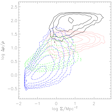
Figure 14: As Fig. 13, but for four distinct populations divided by the mass of the largest dark matter halo in which they are embedded. The lowest contour level represents 10 galaxies per bin (0.1 in the logarithm of $\Sigma$ and $\Delta\rho/\rho$), and the contours are logarithmically spaced by 0.4. The solid contours are restricted to galaxies with $\log{{\cal M}_{halo}/{\cal M}_{\odot}}=14.75\pm 0.1$; the dotted contours represent $\log{\cal M}_{halo}=13.75$, the dashed contours $\log{\cal M}_{halo}=12.75$, and the dash-and-dotted contours $\log{\cal M}_{halo}=11.75$. For halos of fixed mass, $\Sigma$ spans a wide range, as it is sensitive to the local environment of galaxies.

4.2 Comparison between models and data

Recently, Weinmann et al. (2006) have demonstrated that although the models of Croton et al. (2006) do a good job of reproducing the overall luminosity-dependence of the observed galaxy colour distribution, they do not succeed in matching the colour distribution in groups and clusters. Specifically, they found that the model predicts too many faint, red galaxies in these large halos. We will investigate this further by characterising environment using the continuous variable $\Sigma$, which is more closely related to the large-scale dark matter density field than to the mass of the halo.

To divide the model into red and blue galaxies we follow the approach of Weinmann et al. (2006) and make a magnitude-dependent colour cut. We find that a separation at $(B-R)=-0.05\left(M_{r}+20\right)+1.83$ provides a good separation between the red and blue populations of the model (our results below are not sensitive to this cut, because the model populations are so well separated in colour). Figure 15 shows the fraction of red galaxies, using this criterion, as a function of stellar mass and local density $\Sigma$. Qualitatively, the models reproduce the observations well, as the red fraction increases with both stellar mass and $\Sigma$. However, quantitatively there are some interesting differences. In particular, the dependence in the model is actually too strong relative to the data. At low densities, the model predicts too few red galaxies, with a red fraction that varies from 0.05 to 0.6 over the plotted mass range. By contrast, over the same mass range, the data show a red fraction ranging from 0.4 to 1.0. Another point of interest is that the mass dependence of the red fraction in the models is weak below $\sim 10^{10.6}{\cal M}_{\odot}$, while the data show a continuous decrease in red fraction with stellar mass over another order of magnitude. At the high-density end, the models seem to do a better job of reproducing the high red fraction and weak stellar-mass dependence seen in the observations.

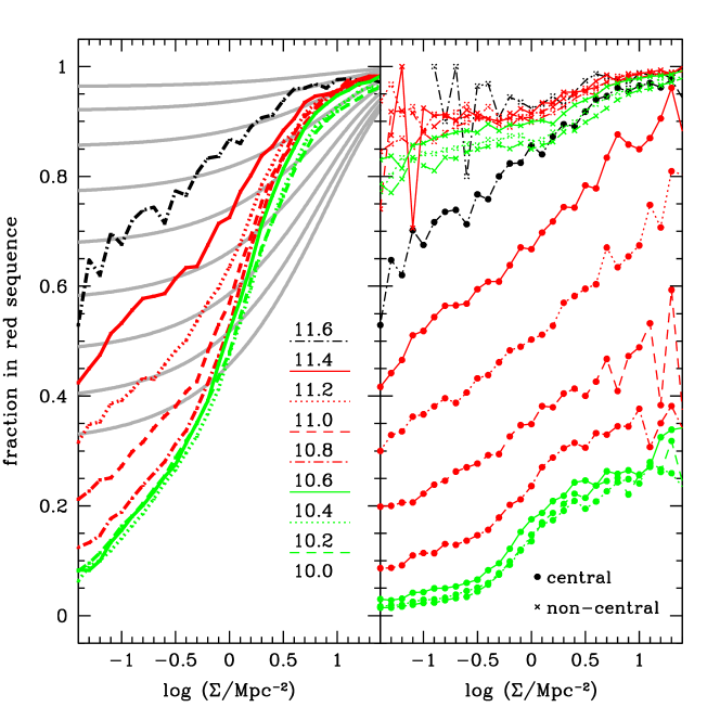
Figure 15: Left panel: The fraction of red galaxies in the Croton et al. (2006) model, as defined in the text, as a function of stellar mass and environment. The green, red and black lines represent the model. They are analogous to those shown in Fig. 11(a) but only extend to masses as low as $10^{10}{\cal M}_{\odot}$. For reference, the grey lines represent $f_{r}$ from the data parameterised using the unified relation of Fig. 12(b) for $\log{\cal M}=10.0$ to 11.6. Right panel: The model galaxies are divided into central galaxies (solid points) and satellite galaxies (crosses).

The main source of the environmental dependence in the model is simply illustrated in the right panel of Fig. 15, where we divide the sample into central and satellite galaxies. As shown by Weinmann et al. (2006), most satellite galaxies are red, independent of luminosity and density, in the models. The central galaxies, on the other hand, have a strong stellar mass dependence, and a dependence on environment that is considerably weaker than that shown by the population as a whole, in the left panel. The overall environmental trend is therefore largely due to the fact that low-density regions are dominated by central galaxies, while the high-density end is dominated by satellite galaxies. The main source of the discrepancy with the observations, therefore, can be identified as the low fraction of red galaxies amongst the central galaxies in low-density environments.

Figure 16 shows the analog of Fig. 15 for the Bower et al. (2006) models. In these models, the colour-luminosity relation is significantly different from Croton et al. (2006), so we have had to adopt a different definition of red galaxy, with a colour cut given by $(B-R)=-0.07\left(M_{r}+20\right)+1.25$. For this model, the agreement with the observations is remarkably good. The difference lies in the colour distribution of the central galaxies, for which, at all densities, a larger fraction lie in the red sequence than in the Croton et al. model. This is not surprising, as the main difference between the two models lies in the treatment of AGN feedback, within central galaxies. Therefore, the satellite populations are largely unaffected.

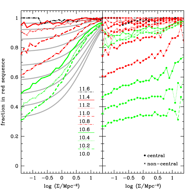
Figure 16: As Fig. 15, but with the galaxy formation model of Bower et al. (2006). The main difference is that the central galaxies have a higher red fraction in all environments, leading to better agreement with the observed, overall environmental trend. The model parameters were not adjusted to match these data.

4.3 Implications

Weinmann et al. (2006) showed that the Croton et al. (2006) model fails to predict the presence of faint blue galaxies in groups and clusters, and link this discrepancy to the uniformly red satellite population that is seen here in both the Croton et al. and Bower et al. (2006) model. This is quite a different effect from the discrepancy revealed by our results, as our data show that the fraction of red galaxies in the densest environments is nearly as high as the models predict. Instead, our analysis shows a problem with the opposite population in the Croton et al. model, in that the central galaxies in low-density environments are too frequently blue. Interestingly, this problem does not appear to be as severe in the Bower et al. model. However, it is not clear whether this improvement is due to their different prescription for AGN feedback, or to some other aspect of the model. Unambiguously identifying the root cause of this difference requires a more detailed comparison between the two models, which is beyond the scope of this paper.

The comparison between models and data that we have discussed and shown in Figs. 15–16 is only the red-blue sequence galaxy fraction; clearly colour-mass, colour-concentration relations and GSMFs could also be compared as a function of environment. However, colour-mass and colour-concentration relations are more dependent on the detailed physics of stellar and galaxy evolution such as chemical and dynamical evolution; whereas the red fraction (based on a colour cut dividing the bimodal population) represents the the most significant variation with environment. The focus of this paper is on the unified relation of the red fraction versus stellar mass and environment, and we have shown that semi-analytical models with their distinction between central and satellite galaxies can match this with an appropriate feedback description (Fig. 16). Of course this does not mean that the Bower et al. (2006) model has the right answer for the galaxy bimodality as there are many other pieces of data to match, e.g., lower mass galaxies, colour relations and GSMFs.

Given that the Bower et al. (2006) model produces a good match to the unified relation we are now in a position to interpret it in the context of the model. In the model, the likelihood that a galaxy lies on the red sequence depends on two factors. Firstly, the probability that the AGN feedback is able to prevent the collapse of further gas depends on the mass and dynamical time of the halo, and the mass of the central black hole. Both of these factors become more effective in larger mass galaxies (through the correlation between central galaxy mass and halo mass, and through the correlation between bulge mass and black hole mass, respectively). Secondly, the probability that a galaxy is a satellite (and therefore unable to accumulate cold gas) increases as $\Sigma$ increases. As the galaxy mass increases, the galaxy is more likely to be central and red regardless of the $\Sigma$ parameter. Conversely the galaxies with the lowest mass are very unlikely to be central if $\Sigma$ is high. Thus the sensitivity to $\Sigma$ depends strongly on galaxy mass, and this dependence is reflected in the unified relation that we have presented.

The success of the model in representing the impact of environment may at first seem surprising since the models presented do not yet include many environment-related process such as ram pressure stripping of cold disk gas and tidal interactions between satellite galaxies. In the models, interaction with the environment occurs because the galaxies external gas reservoir is removed as it becomes a satellite galaxy orbiting within a larger halo. However, because the models assume a rapid interchange between the cold disk gas and the external gas reservoir, the loss of the external halo quickly suppresses the formation of disk stars. It seems that this provides a good approximation to the effect of the complete suite of environmental interactions. The caveat, of course, is that the process (as currently model) seems overly effective so that too few satellite galaxies are able to continue star formation, even in if the parent halo has relatively low mass. Clearly this is an important area in which the models can be developed by introducing a more complete description for the removal of the external reservoir.

5 Summary

We have analysed a primary sample of 151 642 galaxies from the SDSS determining stellar masses, rest-frame colours and projected environmental densities. The peak, or characteristic mass, of the GSMFs increase by about 0.4 dex from $\log\Sigma\simeq-1.2$ to $\log\Sigma\simeq+1.3$ (Fig. 8). The galaxy population is bimodal with a red and blue sequence for which the colour-mass and colour-concentration index relations do not depend strongly on environment (Figs. 9–10). In contrast, the fraction of galaxies on the red sequence depends strongly on both stellar mass and environment (Fig. 11). The stellar-mass and environmental dependence of the red fraction can be unified using empirical laws of the form given by Eqs. 9–10 (Fig. 12).

In order to compare models with the data, we computed the equivalent of galaxy projected neighbour density for semi-analytical models based on the Millennium Simulation. This showed that $\Sigma$ broadly traced the underlying dark-matter density distribution (Figs. 13–14). The fraction of red-sequence galaxies versus stellar mass and environment were computed for two models (Bower et al., 2006; Croton et al., 2006) and compared with the unified relation (Figs. 15–16). Both models produce qualitatively the right trends with environment; with the Bower et al. model providing a good quantitative match.

Appendix A More on the galaxy stellar mass functions

Galaxy luminosity functions and GSMFs are typically fitted using Schechter functions; including galaxy type-dependent functions. There is a logical inconsistency here: the sum of Schechter functions do not sum to a Schechter function in general. The main results in this paper suggest another method of defining type-dependent functions. An overall GSMF is defined by a Schechter-based function while the red- and blue-sequence functions are defined using a probability or fractional function (e.g. Eq. 9 or 10).

Another key point is that an overall luminosity or mass function is in many cases not well parameterised by a standard Schechter function. Modifications to the Schechter function include: adding $\phi_{res}=10^{(a+bM)}$ (Madgwick et al., 2003); adding a Gaussian function (Mercurio et al., 2006); and using a double Schechter function (Paper I) given by

$$\phi_{X}\,{\rm d}X=e^{-X/X^{*}}\left[\phi^{*}_{1}\left(\frac{X}{X^{*}}\right)^{\alpha_{1}}+\phi^{*}_{2}\left(\frac{X}{X^{*}}\right)^{\alpha_{2}}\right]\,\frac{{\rm d}X}{X^{*}}$$ (11)

where $\phi_{X}\,{\rm d}X$ is the number density of galaxies with luminosity or mass between $X$ and $X+{\rm d}X$. One can also specify $\alpha_{2}<\alpha_{1}$ so that the second term will dominate at the faintest magnitudes (cf. Blanton et al. 2005b). The first term then acts to increase the number density around $X^{*}$.

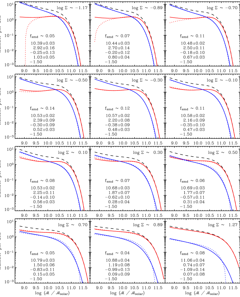
Figure 17: Galaxy stellar mass functions. The dashed lines represent the double Schechter fits to the overall GSMFs. The solid lines represent the red- and blue-sequence GSMFs defined by multiplying the overall fit by $f_{r}$ and $1-f_{r}$ from Eq. 10; while the dotted lines represent the sequences using Eq. 9. Each overall GSMF is normalised to a total mass of $10^{11}\,{\cal M}_{\odot}$. See § 3.3, Fig. 8 and text of Appendix for further details.

The standard Schechter fits are shown in Fig. 8(b) over a reduced mass range. In order to fit the mass functions down to lower masses, we used double Schechter functions with fixed $\alpha_{2}=-1.5$. The fixed faint-end slope was the weighted best-fit average over all environments and was consistent with Blanton et al. (2005b)’s analysis of low-luminosity galaxies. Figure 17 shows the fitted GSMFs for different environments. The red- and blue-sequence GSMFs were then determined by multiplying each overall GSMF by $f_{r}(\Sigma,{\cal M})$ and $1-f_{r}$ from Eq. 9 or 10 with the parameters shown in Fig. 12. The average $\log\Sigma$ value for each environment, the approximate fractional contribution to the stellar mass density ($f_{\rm smd}$) and the double Schechter parameters ($\log{\cal M}^{*},\phi^{*}_{1},\alpha_{1},\phi^{*}_{2},\alpha_{2}$) are shown in each panel. Note with the IMF and mass-to-light ratios used in this paper, $\Omega_{\rm stars}\approx 0.002$ (cf. Persic & Salucci 1992; Baldry & Glazebrook 2003; Nagamine et al. 2006).

References

- Adelman-McCarthy et al. (2006) Adelman-McCarthy J. K., et al., 2006, ApJS, 162, 38
- Alonso et al. (2006) Alonso M. S., Lambas D. G., Tissera P., Coldwell G., 2006, MNRAS, 367, 1029
- Andreon (2004) Andreon S., 2004, A&A, 416, 865
- Andreon (2006) Andreon S., 2006, MNRAS, 369, 969
- Avila-Reese (2006) Avila-Reese V., 2006, in Carramiñana A., et al. eds, Proc. IV Mexican School of Astrophysics. Springer, in press (astro-ph/0605212)
- Baldry & Glazebrook (2003) Baldry I. K., Glazebrook K., 2003, ApJ, 593, 258
- Baldry et al. (2004a) Baldry I. K., Glazebrook K., Brinkmann J., Ivezić Ž., Lupton R. H., Nichol R. C., Szalay A. S., 2004a, ApJ, 600, 681 (Paper I)
- Baldry et al. (2004b) Baldry I. K., Balogh M. L., Bower R., Glazebrook K., Nichol R. C., 2004b, in Allen R. E., et al. eds, AIP Conf. Proc. Vol. 743. AIP, Melville, NY, p. 106
- Ball et al. (2006) Ball N. M., Loveday J., Brunner R. J., Baldry I. K., Brinkmann J., 2006, MNRAS, in press (astro-ph/0507547)
- Balogh et al. (2001) Balogh M. L., Christlein D., Zabludoff A. I., Zaritsky D., 2001, ApJ, 557, 117
- Balogh et al. (2004a) Balogh M. L., et al., 2004a, MNRAS, 348, 1355 (Paper II)
- Balogh et al. (2004b) Balogh M. L., Baldry I. K., Nichol R., Miller C., Bower R., Glazebrook K., 2004b, ApJ, 615, L101 (Paper III)
- Bell & de Jong (2001) Bell E. F., de Jong R. S., 2001, ApJ, 550, 212
- Bell et al. (2003) Bell E. F., McIntosh D. H., Katz N., Weinberg M. D., 2003, ApJS, 149, 289
- Benson et al. (2002) Benson A. J., Frenk C. S., Sharples R. M., 2002, ApJ, 574, 104
- Bernardi et al. (2006) Bernardi M., Nichol R. C., Sheth R. K., Miller C. J., Brinkmann J., 2006, AJ, 131, 1288
- Binggeli et al. (1988) Binggeli B., Sandage A., Tammann G. A., 1988, ARA&A, 26, 509
- Binney (2004) Binney J., 2004, MNRAS, 347, 1093
- Birnboim & Dekel (2003) Birnboim Y., Dekel A., 2003, MNRAS, 345, 349
- Blanton et al. (2001) Blanton M. R., et al., 2001, AJ, 121, 2358
- Blanton et al. (2003a) Blanton M. R., Lin H., Lupton R. H., Maley F. M., Young N., Zehavi I., Loveday J., 2003a, AJ, 125, 2276
- Blanton et al. (2003b) Blanton M. R., et al., 2003b, AJ, 125, 2348
- Blanton et al. (2003c) Blanton M. R., et al., 2003c, ApJ, 592, 819
- Blanton et al. (2005a) Blanton M. R., Eisenstein D., Hogg D. W., Schlegel D. J., Brinkmann J., 2005a, ApJ, 629, 143
- Blanton et al. (2005b) Blanton M. R., Lupton R. H., Schlegel D. J., Strauss M. A., Brinkmann J., Fukugita M., Loveday J., 2005b, ApJ, 631, 208
- Blanton et al. (2006) Blanton M. R., Eisenstein D., Hogg D. W., Zehavi I., 2006, ApJ, 645, 977
- Bower (1991) Bower R. G., 1991, MNRAS, 248, 332
- Bower et al. (2006) Bower R. G., Benson A. J., Malbon R., Helly J. C., Frenk C. S., Baugh C. M., Cole S., Lacey C. G., 2006, MNRAS, 370, 645
- Brinchmann & Ellis (2000) Brinchmann J., Ellis R. S., 2000, ApJ, 536, L77
- Cattaneo et al. (2006) Cattaneo A., Dekel A., Devriendt J., Guiderdoni B., Blaizot J., 2006, MNRAS, 370, 1651
- Chester & Roberts (1964) Chester C., Roberts M. S., 1964, AJ, 69, 635
- Cole et al. (2000) Cole S., Lacey C. G., Baugh C. M., Frenk C. S., 2000, MNRAS, 319, 168
- Conselice et al. (2005) Conselice C. J., Bundy K., Ellis R. S., Brichmann J., Vogt N. P., Phillips A. C., 2005, ApJ, 628, 160
- Cooper et al. (2006) Cooper M. C., et al., 2006, MNRAS, 370, 198
- Croton et al. (2005) Croton D. J., et al., 2005, MNRAS, 356, 1155
- Croton et al. (2006) Croton D. J., et al., 2006, MNRAS, 365, 11
- De Lucia et al. (2004) De Lucia G., et al., 2004, ApJ, 610, L77
- De Propris et al. (2003) De Propris R., et al., 2003, MNRAS, 342, 725
- Dekel & Birnboim (2006) Dekel A., Birnboim Y., 2006, MNRAS, 368, 2
- Dressler (1980) Dressler A., 1980, ApJ, 236, 351
- Driver et al. (2006) Driver S. P., et al., 2006, MNRAS, 368, 414
- Eisenstein et al. (2001) Eisenstein D. J., et al., 2001, AJ, 122, 2267
- Ellis et al. (2005) Ellis S. C., Driver S. P., Allen P. D., Liske J., Bland-Hawthorn J., De Propris R., 2005, MNRAS, 363, 1257
- Faber (1973) Faber S. M., 1973, ApJ, 179, 731
- Felten (1976) Felten J. E., 1976, ApJ, 207, 700
- Gómez et al. (2003) Gómez P. L., et al., 2003, ApJ, 584, 210
- Gallazzi et al. (2005) Gallazzi A., Charlot S., Brinchmann J., White S. D. M., Tremonti C. A., 2005, MNRAS, 362, 41
- Glazebrook et al. (2004) Glazebrook K., et al., 2004, Nature, 430, 181
- Gray et al. (2004) Gray M. E., Wolf C., Meisenheimer K., Taylor A., Dye S., Borch A., Kleinheinrich M., 2004, MNRAS, 347, L73
- Gunn et al. (1998) Gunn J. E., et al., 1998, AJ, 116, 3040
- Haines et al. (2006) Haines C. P., Merluzzi P., Mercurio A., Gargiulo A., Krusanova N., Busarello G., La Barbera F., Capaccioli M., 2006, MNRAS, 371, 55
- Hogg et al. (2002) Hogg D. W., et al., 2002, AJ, 124, 646
- Hogg et al. (2003) Hogg D. W., et al., 2003, ApJ, 585, L5
- Hogg et al. (2004) Hogg D. W., et al., 2004, ApJ, 601, L29
- Holmberg (1958) Holmberg E., 1958, Meddelanden Lunds Astron. Obser. Ser. II, 136, 1
- Hoyle et al. (2005) Hoyle F., Rojas R. R., Vogeley M. S., Brinkmann J., 2005, ApJ, 620, 618
- Ilbert et al. (2006) Ilbert O., et al., 2006, A&A, submitted (astro-ph/0602329)
- Jester et al. (2005) Jester S., et al., 2005, AJ, 130, 873
- Kang et al. (2005) Kang X., Jing Y. P., Mo H. J., Börner G., 2005, ApJ, 631, 21
- Kauffmann et al. (2003a) Kauffmann G., et al., 2003a, MNRAS, 341, 33
- Kauffmann et al. (2003b) Kauffmann G., et al., 2003b, MNRAS, 341, 54
- Kauffmann et al. (2004) Kauffmann G., White S. D. M., Heckman T. M., Ménard B., Brinchmann J., Charlot S., Tremonti C., Brinkmann J., 2004, MNRAS, 353, 713
- Kelm et al. (2005) Kelm B., Focardi P., Sorrentino G., 2005, A&A, 442, 117
- Kereš et al. (2005) Kereš D., Katz N., Weinberg D. H., Davé R., 2005, MNRAS, 363, 2
- Kodama et al. (2004) Kodama T., et al., 2004, MNRAS, 350, 1005
- Kroupa (2001) Kroupa P., 2001, MNRAS, 322, 231
- Lewis et al. (2002) Lewis I. J., et al., 2002, MNRAS, 333, 279
- Li et al. (2006) Li C., Kauffmann G., Jing Y. P., White S. D. M., Börner G., Cheng F. Z., 2006, MNRAS, 368, 21
- Madgwick et al. (2003) Madgwick D. S., et al., 2003, ApJ, 599, 997
- Mandelbaum et al. (2006) Mandelbaum R., Seljak U., Kauffmann G., Hirata C. M., Brinkmann J., 2006, MNRAS, 368, 715
- Mateus et al. (2006) Mateus A., Sodre L. J., Cid Fernandes R., Stasinska G., 2006, MNRAS, submitted (astro-ph/0604063)
- Maulbetsch et al. (2006) Maulbetsch C., Avila-Reese V., Colin P., Gottloeber S., Khalatyan A., Steinmetz M., 2006, ApJ, submitted (astro-ph/0606360)
- Menci et al. (2005) Menci N., Fontana A., Giallongo E., Salimbeni S., 2005, ApJ, 632, 49
- Menci et al. (2006) Menci N., Fontana A., Giallongo E., Grazian A., Salimbeni S., 2006, ApJ, 647, 753
- Mercurio et al. (2006) Mercurio A., et al., 2006, MNRAS, 368, 109
- Nagamine et al. (2006) Nagamine K., Ostriker J. P., Fukugita M., Cen R., 2006, ApJ, submitted (astro-ph/0603257)
- Pannella et al. (2006) Pannella M., Hopp U., Saglia R. P., Bender R., Drory N., Salvato M., Gabasch A., Feulner G., 2006, ApJ, 639, L1
- Patiri et al. (2006) Patiri S. G., Prada F., Holtzman J., Klypin A., Betancort-Rijo J., 2006, MNRAS, submitted (astro-ph/0605703)
- Perez et al. (2006) Perez M. J., Tissera P. B., Scannapieco C., Lambas D. G., De Rossi M. E., 2006, A&A, in press (astro-ph/0605131)
- Pérez-González et al. (2003) Pérez-González P. G., Gallego J., Zamorano J., Alonso-Herrero A., Gil de Paz A., Aragón-Salamanca A., 2003, ApJ, 587, L27
- Persic & Salucci (1992) Persic M., Salucci P., 1992, MNRAS, 258, 14P
- Postman & Geller (1984) Postman M., Geller M. J., 1984, ApJ, 281, 95
- Prugniel & Simien (1996) Prugniel P., Simien F., 1996, A&A, 309, 749
- Richards et al. (2002) Richards G. T., et al., 2002, AJ, 123, 2945
- Roberts & Haynes (1994) Roberts M. S., Haynes M. P., 1994, ARA&A, 32, 115
- Schechter (1976) Schechter P., 1976, ApJ, 203, 297
- Schlegel et al. (1998) Schlegel D. J., Finkbeiner D. P., Davis M., 1998, ApJ, 500, 525
- Springel et al. (2005a) Springel V., et al., 2005a, Nature, 435, 629
- Springel et al. (2005b) Springel V., Di Matteo T., Hernquist L., 2005b, ApJ, 620, L79
- Stoughton et al. (2002) Stoughton C., et al., 2002, AJ, 123, 485
- Strateva et al. (2001) Strateva I., et al., 2001, AJ, 122, 1861
- Strauss et al. (2002) Strauss M. A., et al., 2002, AJ, 124, 1810
- Tanaka et al. (2004) Tanaka M., Goto T., Okamura S., Shimasaku K., Brinkmann J., 2004, AJ, 128, 2677
- Thomas et al. (2005) Thomas D., Maraston C., Bender R., de Oliveira C. M., 2005, ApJ, 621, 673
- Thronson & Greenhouse (1988) Thronson H. A., Greenhouse M. A., 1988, ApJ, 327, 671
- Tully et al. (1982) Tully R. B., Mould J. R., Aaronson M., 1982, ApJ, 257, 527
- Weinmann et al. (2006) Weinmann S. M., van den Bosch F. C., Yang X., Mo H. J., Croton D. J., Moore B., 2006, MNRAS, submitted (astro-ph/0606458)
- Whitmore & Gilmore (1991) Whitmore B. C., Gilmore D. M., 1991, ApJ, 367, 64
- Wild et al. (2005) Wild V., et al., 2005, MNRAS, 356, 247
- Wilman et al. (2005) Wilman D. J., et al., 2005, MNRAS, 358, 88
- Yee et al. (2005) Yee H. K. C., Hsieh B. C., Lin H., Gladders M. D., 2005, ApJ, 629, L77
- York et al. (2000) York D. G., et al., 2000, AJ, 120, 1579
- Zandivarez et al. (2006) Zandivarez A., Martinez H. J., Merchan M. E., 2006, ApJ, submitted (astro-ph/0602405)
- Zehavi et al. (2005) Zehavi I., et al., 2005, ApJ, 630, 1