Dark matter and dark energy as a effects of Modified Gravity

Abstract

We explain the effect of dark matter (flat rotation curve) using modified gravitational dynamics. We investigate in this context a low energy limit of generalized general relativity with a nonlinear Lagrangian ${\cal L}\propto R^{n}$, where $R$ is the (generalized) Ricci scalar and $n$ is parameter estimated from SNIa data. We estimate parameter $\beta$ in modified gravitational potential $V(r)\propto-\frac{1}{r}(1+(\frac{r}{r_{c}})^{\beta})$. Then we compare value of $\beta$ obtained from SNIa data with $\beta$ parameter evaluated from the best fitted rotation curve. We find $\beta\simeq 0.7$ which becomes in good agreement with an observation of spiral galaxies rotation curve. We also find preferred value of $\Omega_{m,0}$ from the combined analysis of supernovae data and baryon oscillation peak. We argue that although amount of ”dark energy” (of non-substantial origin) is consistent with SNIa data and flat curves of spiral galaxies are reproduces in the framework of modified Einstein’s equation we still need substantial dark matter. For comparison predictions of the model with predictions of the $\Lambda$CDM concordance model we apply the Akaike and Bayesian information criteria of model selection.

1 Introduction

Different astronomical observations [1, 2] are pointing out that our Universe becomes, at present time, in accelerating phase of expansion. In principle, there are two quite different approaches to explain this observational fact. In the first approach (which can be called substantial) it is assumed that universe is filled by mysterious perfect fluid violating the strong energy condition $\rho_{x}+3p_{x}>0$, where $\rho_{x}$ and $p_{x}$ are, respectively, the energy density and the pressure of this fluid. The nature as well as origin of this matter, called dark energy, is unknown until now. Among these approaches have appeared concordance $\Lambda$CDM model, which predicts that baryons contribute only about 4% of the critical energy density, non-baryonic cold dark matter (CDM) about 25% and the cosmological constant $\Lambda$ (vacuum energy) remaining 70%. Although $\Lambda$CDM model fits well SNIa data [3, 4] this model offers only description of the observations not their explanation. From the methodological view point the conception of mysterious dark energy seems to be effective physical theory only and motivates theorists for searching of alternative approaches in which nature of dark energy will be known at the very beginning.

In the first approach it is assumed that Einstein’s theory of general relativity is valid which reduces in practice (after assuming Robertson-Walker symmetry of space slices) to the case of Friedman - Robertson - Walker models. Nevertheless, theoretically it is not a’priori excluded the possibility of cosmology based on some extension of Einstein’s general relativity. In this paper we consider such particular cases.

On the other hand, there are alternative ideas of explanation, in which instead of dark energy some modifications of Friedmann’s equation are proposed at the very beginning. In these approaches some effects arising from new physics like brane cosmologies, quantum effects, nonhomogeneities effects etc. can mimic dark energy by a modification of Friedmann equation. Freese & Lewis [5] have shown that contributions of type $\rho^{n}$ to Friedmann’s equation $3H^{2}=\rho_{\mathrm{eff}}$, where $\rho_{\mathrm{eff}}$ is the effective energy density and $n$ is a constant, may describe such situations phenomenologically. These models (called by their authors called the Cardassian models) give rise to acceleration, although the universe is flat, contains the usual matter and radiation without any dark energy components. This models have been tested by many authors (see for example [6, 7, 8, 9, 10, 11, 12]). What is still lacking is a fundamental theory (like general relativity) from which these models can be derived after postulating Robertson Walker symmetry.

In this paper we shall consider such particular type of generalization of Einstein’s general relativity in which Lagrangian is proportional to $R^{n}$, where $R$ is generalized Ricci skalar. In particular, Einstein’s general relativity is recovered if we put $n=1$. This theory is part of the larger class of so-called f(R) gravity, i.e. theories derived from gravitational Lagrangians that are analytical (usually polynomial) functions of $R$. (see e.g. [13, 14, 15, 16, 17, 18, 19, 20, 21]. In this approach (we called it non-substantial) instead of postulating mysterious dark energy it is assumed some extension of general relativity. Then effect of acceleration appeared naturally as a dynamical effect of the model. For modified gravity one can find Newtonian potential in non-relativistic limit and ask about possibility to explain flat rotation curve of spiral galaxies - major evidence for dark matter in the universe [22, 23, 24]. (However, see also [25] for non flat rotational curves.) The main goal here is to explore power of this particular generalization of gravity in the context of dark energy and dark matter problems. We argue that although cosmology with modified Lagrangian ${\cal L}\propto R^{n}$ can explain ”dark energy problem” but baryon oscillation test distinguishes value of density parameter of mater to be equal $\Omega_{m,0}\simeq 0.3$, i.e. problem of dark matter is yet not solved within the framework of f(R) theories. We also demonstrate that models under considerations can reproduce rotation curves of spiral galaxies.

The structure of the paper is as follows. In section II we define class of cosmological models of essential theory of gravity with lagrangian proportional to the Ricci scalar. Section III is devoted to analyze constraints on model parameters from SNIa, baryon oscillation peak and CMB shift. In section IV we investigate problem of rotation curves of spiral galaxies. Section V summarizes our results and formulates general conclusion that models modified gravity which are based on generalized lagrangians ${\cal L}\propto R^{n}$ and Palatini formalism although solve the acceleration and flat rotation curves problems still favor $\Omega_{m,0}\simeq 0.3$.

2 Cosmological models of nonlinear Palatini gravity

Let us consider the simplest cosmological model of generalized Einstein’s theory of gravity with Lagrangian ${\cal L}=f(R)$ which is function of the (generalized) Ricci scalar. The action is assumed in the form

$$A=A_{\mathrm{grav}}+A_{\mathrm{mat}}=\int(\sqrt{\det g}f(R)+2L_{\mathrm{mat}}(\Psi))d^{4}x$$ (1)

where $f(R)\propto R^{n}$ and $n$ is a constant. We also assumed that dynamical equation determining evolution of the cosmological model can be derived from the action through the Palatini formalism in which both metric $g$ and symmetric connection $\Gamma$ are regarded as an independent variables. Thus $R\equiv R(g,\Gamma)=g^{\mu\nu}R_{\mu\nu}(\Gamma)$ denotes generalized Ricci scalar (see e.g. [17] for details).

Because of homogeneity and isotropy of the surface $t=const$ is assumed, $t$ - being a global cosmic time, we choose Robertson-Walker metric i.e.

$$ds^{2}=-dt^{2}+a^{2}(t)\Big{[}{1\over{1-kr^{2}}}dr^{2}+r^{2}\Big{(}d\theta^{2}+\sin^{2}(\theta)d\varphi^{2}\Big{)}\Big{]}\ .$$ (2)

where $k=0,\pm 1$ is curvature index, $r,\theta,\phi$ are usual spherical coordinates. Some properties of these theories (in the Palatini framework) have been already investigated by Capozziello et al. [26]. It has been demonstrated that under two popular choices $f(R)\propto R^{n}$ and $f(R)\propto\ln R$ both models provide well fits to the SNIa data.

Here we consider matter content in the form of perfect fluid which satisfy the conservation condition:

$$\frac{d\rho}{dt}=-3H(\rho+p)$$ (3)

where $H=\frac{d}{dt}(\ln a)$ is Hubble’a function. For convenience we assume simple form of equation of state (E.Q.S). After adopting Palatini formalism field equation reduces to the ordinary second order differential equation which admits first integral in the form:

$$H^{2}=F(a).$$ (4)

The first integral (4) is usually called (generalized) Friedman equation. This is the first order differential equation in which right hand side is determined by matter content and curvature. Due to simple relation between the scale factor and the redshift $z$ ($1+z=\frac{a_{0}}{a}$) formula (4) can be written in the form $H^{2}=F(z)$ ($a_{0}$ denotes the present value of the scale factor which corresponds to the redshift $z=0$) In the system filled by both dust matter and radiation the function $F(a)$ takes the following form:

$$H^{2}=\frac{2n}{3(3-n)}\left[\frac{\kappa\eta_{dust}}{\beta}\right]^{\frac{1}{n}}\,a^{-\frac{3}{n}}+$$

$$+\frac{4n(2-n)\kappa\eta_{rad}}{3\beta(n-3)^{2}}\left[\frac{\kappa\eta_{dust}}{\beta}\right]^{\frac{1-n}{n}}\,a^{-\frac{n+3}{n}}-\frac{k}{a^{2}}\,\left[\frac{2n}{(n-3)}\right]^{2}\ .$$ (5)

where $\mathcal{L}_{\mathrm{grav}}=\frac{\beta}{2-n}R^{n}\sqrt{g}$, $\beta$ is dimensional constant, $w_{dust}\equiv p_{dust}/\rho_{dust}=0$. If $n=\beta=1$ and $\eta_{rad}=0$ then the classical FRW dust filled model is recovered.

Let us formulate some important remarks:

1. the formula (5) contains many nonphysical parameters which can be replaced by dimensionless density parameters $\Omega_{i}$ defined for each additive contribution to the r.h.s. of (4). This in turn can be treated as a (fictitious or real) component of some effective energy density. Density parameter $\Omega_{i}$ is defined for each energy component in standard way $\Omega_{i}=\rho_{i}/3H_{0}^{2}$ where $H_{0}$ is present value of the Hubble function and $\rho_{i}$ is energy density of $i-th$ fluid.

2. for our further analysis it is useful to separate this contribution on the r.h.s. of (4) which represents real dust matter scaling like $a^{-3}$ from the non-substantial effects of generalized Lagrangian (related with n-parameter). Then our basic formula can be rewritten to the new more suitable form:

   $$\left(\frac{H}{H_{0}}\right)^{2}=\Omega_{m,0}(1+z)^{3}\frac{2n}{\left(3-n\right)}\Omega_{nonl,0}(1+z)^{\frac{3\left(1-n\right)}{n}}+$$

   $$+\Omega_{r,0}(1+z)^{4}\frac{4n\left(2-n\right)}{\left(n-3\right)^{2}}\Omega_{nonl,0}(1+z)^{\frac{3\left(1-n\right)}{n}}\ .$$ (6)

   where parameter $\Omega_{nonl,0}$ is determined from the constraint $H(z=0)=H_{0}$

   $$\Omega_{nonl,0}=\left(\frac{2n}{\left(3-n\right)}\Omega_{m,0}+\frac{4n\left(2-n\right)}{\left(n-3\right)^{2}}\Omega_{r,0}\right)^{-1}\ .$$ (7)

   Here $k=0$ is assumed for simplicity (for more general formulas see [27]).

One can check that in the case of $n=1$ one obtains Einstein de Sitter model filled with matter and radiation. The basic formula (6) will be suitable in the next section for providing priors on $\Omega_{m,0}$ which can be obtained from independent extragalactic measurements or baryon oscillation peak.

From formula (6) on can drive a few conclusions. The first is that rejection of $\Omega_{r,0}$ in (6) doesn’t eliminate automatically the dust term. On the other hand substitution $\eta_{dust}=0$ give rise to rejection of the second (radiation) term automatically. The next observation arising from (6) is that term $\Omega_{nonl,0}(1+z)^{\frac{3\left(1-n\right)}{n}}$ plays a role of lapse function. Therefore one can re-scale original cosmological time following the rule: $t\mapsto\tau$: $d\tau^{2}=\Omega_{nonl,0}(1+z)^{\frac{3\left(1-n\right)}{n}}dt^{2}$ and then obtain, after re-scaling density parameters, a flat model which is dynamically equivalent to the flat FRW model with : $\overline{\Omega_{m,0}}=\Omega_{m,0}\frac{2n}{3-n}$ and $\overline{\Omega_{r,0}}=\Omega_{r,0}\frac{4n\left(2-n\right)}{\left(3-n\right)^{2}}$. Therefore, the exact solutions are well known in the form of $t=t(\overline{\Omega_{m,0}},\overline{\Omega_{r,0}},z)$.

It is also worth to notice that equation (6) is equivalent to

$$\left(\frac{H}{H_{0}}\right)^{2}-F(a)\equiv 0\qquad\mathrm{or}\qquad\frac{\left(a^{{}^{\prime}}\right)^{2}}{2}+V(a)=0,$$ (8)

where ${}^{\prime}\equiv\frac{d}{d\tau}$, $dt|H_{0}|=d\tau$, $V(a)=-\rho_{eff}\frac{a^{2}}{6}=\frac{-F(a)a^{2}}{2}$. Due to particle like representation of the dynamics in the form (8) it is possible its investigation in terms of what H.-J. Schmidt calls classical mechanics with the lapse function [28].

3 Observational constraints on modified gravity parameters

Within the framework of modified gravity, the acceleration originates from non-substantial contribution arising from curvature modification. This gives rise to negative effective pressure and leads to self accelerating cosmology.

3.1 Constraining model parameters from SNIa data

The fundamental test for parameters of cosmological model is based on the luminosity distance as a function of red-shift $d_{l}(z)$ (the so-called Hubble diagram)

$$d_{L}(z)=(1+z)\frac{c}{H_{0}}\frac{1}{\sqrt{|\Omega_{k,0}|}}\mathcal{F}\left(H_{0}\sqrt{|\Omega_{k,0}|}\int_{0}^{z}\frac{dz^{\prime}}{H(z^{\prime})}\right)\ ,$$ (9)

where $\Omega_{k,0}=-\frac{k}{H_{0}^{2}}$ and $\mathcal{F}(x)\equiv\sinh(x),x,\sin(x)\qquad\mathrm{for}\qquad k=-1,0,+1$ respectively. For distant SNIa relation between luminosity distance $d_{L}$, absolute magnitude $M$ and directly observed their apparent magnitude $m$ has the following form:

$$\mu\equiv m-M=5\log_{10}d_{L}+25=5\log_{10}D_{L}+\mathcal{M}\ ,$$ (10)

where $\mathcal{M}=-5\log_{10}H_{0}+25$ and $D_{L}=H_{0}d_{L}$.

The goodness of fit is characterized by the parameter

$$\chi^{2}=\sum_{i}\frac{(\mu_{i}^{\mathrm{theor}}-\mu_{i}^{\mathrm{obs}})^{2}}{\sigma_{i}^{2}}\ .$$ (11)

where $\mu_{i}^{\mathrm{obs}}$ is the measured value, $\mu_{i}^{\mathrm{theor}}$ is the value calculated in the model under consideration, and $\sigma_{i}$ is the total measurement error. Assuming that supernovae measurements come with uncorrelated Gaussian errors, one can determine the likelihood function $\mathcal{L}\propto\exp(-\chi^{2}/2)$. The Probability Density Function (PDF) of cosmological parameters [1] can be derived from Bayes’ theorem. Therefore, one can estimate model parameters by using a minimization procedure. It is based on the likelihood function as well as on the best fit method minimizing $\chi^{2}$.

In our analysis we used two samples of supernovae. One of them is “Gold” Riess et al. sample of 157 SNIa [3]. Second one is the sample of 115 supernovae compiled recently by Astier et al. [4]. This latest sample of 115 supernovae is our basic sample.

For statistical analysis we have restricted the parameter $\Omega_{m,0}$ to the interval $[0,1]$ and $n$ to $[-10.0,10.0]$ (except $n=0$ and additionally $n=3$ for $w=0$). Moreover, because of the singularity at $n=3,w=0$ we have separated the cases $n>3$ and $n<3$ for $w=0$ in our analysis. Please note that $\Omega_{nonl,0}$ is obtained from the constraint $H(z=0)=H_{0}$. The results of two fitting procedures performed on Riess and Astier samples with different prior assumptions for $n$ are presented in Tables 1 and 2. In the Table 1 the values of model parameters obtained from the minimum the $\chi^{2}$ are given, whereas in Table 2 the results from marginalized probability density functions are displayed. The best fit (minimum $\chi^{2}$) gives $n\simeq 2.6$ with the Astier et al. sample versus $n\simeq 2.1$ with the Gold sample. In Figure 1 we present Probability distribution obtained with the Astier sample for the parameters $\Omega_{m,0}$ and $n$ for non-linear gravity model, (case $n<3$ marginalized over the rest of parameters). Please note that from Fig. 1 we obtain a very weak dependence of PDF on the matter density parameter if only $\Omega_{m,0}\geq 0.05$. Because bounce is a generic features of presented models for $n>2$ [27] it is interesting to calculate from observational data probability that value of $n$ paprameter is greated from two. We find that $P(n>2)\simeq 0.99$. It means that bounce is strongly favored over big-bang scenario like to in loop quantum gravity for example [32]. The Fig. 2 and Fig. 3 shows likelihood contours on the plane $(\Omega_{m,0},n)$ obtained (from fits to the SNIa data and baryon oscilation peak test respecitvely), obtained for non-linear gravity model, for the case $n<3$ marginalized over ${\cal M}$

Table 1: The flat non-linear gravity model with dust and radiation. Results of statistical analysis performed with Astier et al. and Gold Riess et al. samples of SNIa as a minimum $\chi^{2}$ best-fit. We separately analyzed the case $n>3$ and $n<3$ .

sample	$\Omega_{m,0}$	$\Omega_{nonl,0}$	$n$	$\chi^{2}$
Gold	0.35	$<0.01$	3.001	180.7
$n<3$	0.89	$0.23$	2.13	181.5
$n>3$	0.35	$<0.01$	3.001	180.7
Astier	0.01	$-1.47$	3.11	108.7
$n<3$	0.98	$0.08$	2.59	108.9
$n>3$	0.01	$-1.47$	3.11	108.7

Table 2: The flat non-linear gravity cosmological model with dust and radiation. The values of the parameters obtained from one dimensional PDFs calculated on the Astier et al. and the Gold Riess et al. SNIa samples. Because of the singularity at $n=3$ we separately analyze the cases $n>3$ and $n<3$ .

sample	$\Omega_{m,0}$	$\Omega_{nonl,0}$	$n$
Gold	$0.01$	$0.26$	$2.11$
$n<3$	$1.00$	$0.26$	$2.11$
$n>3$	$0.01$	$-0.01$	$3.001$
Astier	$0.01$	$0.09$	$2.56$
$n<3$	$1.00$	$0.09$	$2.56$
$n>3$	$0.01$	-$0.01$	$3.01$

Figure 1: Probability distribution obtained with the Astier sample for the parameters $\Omega_{m,0}$ and $n$, marginalized over the rest of parameters. Non-linear gravity model, $n<3$ .

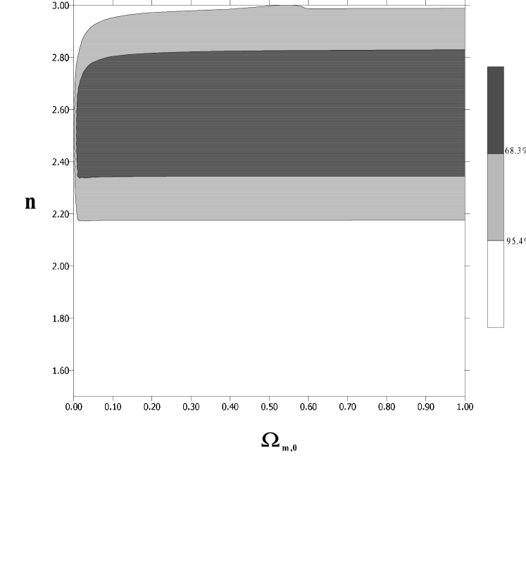
Figure 2: The flat non-linear gravity model with dust and radiation ($n<3$). Likelihood contours on the $(\Omega_{m,0},n)$ plane, marginalized over ${\cal M}$, obtained from fits to SNIa Astier et al. sample.

Most popular are the Akaike information criteria (AIC) [33] and the Bayesian information criteria (BIC) [34]. We use this criteria to select model parameters providing the preferred fit to data.

One of the important problem of modern observational cosmology is the so-called degeneracy problem: many models with dramatically different scenarios agree with the present day observational data. Information criteria for model selection [29] can be used, in some subclass of dark energy models, in order to overcome this degeneracy [30, 31]. Most popular are the Akaike information criteria (AIC) [33] and the Bayesian information criteria (BIC) [34]. We use this criteria to select model parameters providing the preferred fit to data.

The AIC [33] is defined by

$$\mathrm{AIC}=-2\ln{\mathcal{L}}+2d\ ,$$ (12)

where $\mathcal{L}$ is the maximum likelihood and $d$ the number of model parameters. The best model, with a parameter set providing the preferred fit to the data, is that which minimizes the AIC.

The BIC introduced by Schwarzc [34] is defined as

$$\mathrm{BIC}=-2\ln{\mathcal{L}}+d\ln{N}\ ,$$ (13)

where $N$ is the number of data points used in the fit. While AIC tends to favor models with a large number of parameters, the BIC penalizes them more strongly, so the later provides a useful approximation to the full evidence in the case of no prior on the set of model parameters [35].

Please note that both values of information criteria have no absolute sense and only the relative values between different models are physically interesting. For the BIC a difference of $2$ is treated as a positive evidence ($6$ as a strong evidence) against the model with larger value of BIC [36, 37]. If we do not find any positive evidence from information criteria, the models are treated as identical, while eventually additional parameters are treated as not significant. Therefore, the information criteria offer a possibility to introduce a relation of weak ordering among considered models.

Table 3: Results of AIC and BIC performed on the Astier versus the Gold Riess samples of SNIa.

sample	AIC	BIC
$\Lambda$CDM Gold	179.9	186.0
$\Lambda$CDM Astier	111.8	117.3
Non-Lin.Grav. Gold	186.6	195.8
Non-Lin.Grav. Astier	114.7	122.9

In the Table 3 the value of AIC and BIC for the $\Lambda$CDM and the non-linear gravity models are presented. Note that for both samples we obtain with AIC and BIC for the $\Lambda$CDM model smaller values than for non-linear gravity. Most interst is using a Bayesian framework to compare the cosmological models, because they automatically penalize models with more parameters to fit the data. Based on these simple information criteria, we find that the SNIa data still favor the $\Lambda$CDM model, because under a similar quality of the fit for both models, the $\Lambda$CDM contains less parameters.

3.2 CMB shift parameter

For stringent and deeper constraint on model parameters we include in our analysis the so called (CMB) ”shift parameter“. This parameter is defined as:

$$R\equiv\sqrt{\frac{\Omega_{m,0}}{|\Omega_{k,0}|}}\mathcal{F}\left(y(z_{lss})\right)$$ (14)

where $R_{0}=1.716\pm 0.062$ [38] and $z_{lss}=1089$ [39]. The $R$-parameter determines the angular scale of the first acustic peak through the angular distance to last scattering and physical scale of the sound horizon. It is insensitive with respect perturbations and are suitable to constrain model parameter. The region allowed by the analysis of (CMB) ”shift parameter“ the plane $(\Omega_{m,0},n)$ for non-linear gravity model (for the case $n<3$) is presented on the Fig 4 (lower panel).

We obtain for non-linear gravity model the values of the model parameters $\Omega_{m,0}=0.67$ and $n=1.03$ as a best fit. Please note that this area is not allowed by SNIa data.

3.3 Baryon oscillation peak

Recently Fairbarn and Goobar [40] used baryon oscillation peak detected in the SDSS Luminosity Red Galaxies Survey [41] as a independent test of Dvali-Gabadadze-Porrati (DGP) brane model. They used constraint for:

$$A\equiv=\frac{\sqrt{\Omega_{m,0}}}{E(z_{1})^{\frac{1}{3}}}\left(\frac{1}{z_{1}\sqrt{|\Omega_{k,0}|}}\mathcal{F}\left(\sqrt{|\Omega_{k,0}|}\int_{0}^{z_{1}}\frac{dz}{E(z)}\right)\right)^{\frac{2}{3}}\ ,$$ (15)

so that $E(z)\equiv H(z)/H_{0}$ and $z_{1}=0.35$ yield $A=0.469\pm 0.017$. The quoted uncertainty corresponds to one standard deviation, where a Gaussian probability distribution has been assumed. These constraints could be used for fitting cosmological parameters (see also [4, 40, 42]).

Fairbarn and Goobar [40] showed that the joint constraints for both SNIA data and the baryon oscillations peak ruled out flat DGP model at the 99% confidence level. Analogical analysis can be performed for our model. We obtain for non-linear gravity model the values of the model parameters $\Omega_{m,0}=0.28$, $\Omega_{nonl,0}=0.33$ and $n=2.53$ as a best fit. On the Fig.3 we show the region allowed by the baryon oscillation test on the plane $(\Omega_{m,0},n)$ for non-linear gravity model with dust and radiation (for the case $n<3$).

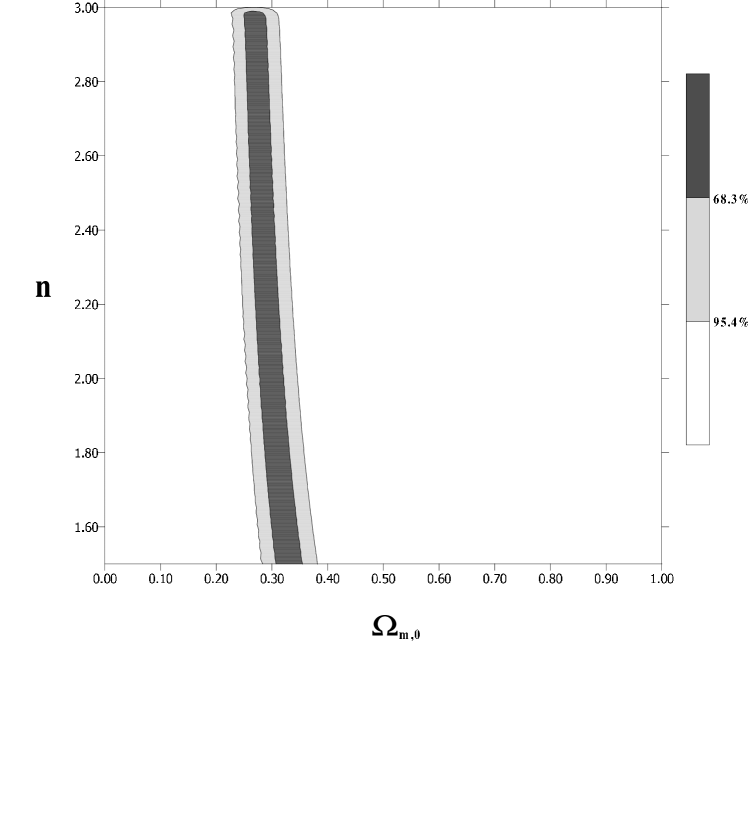
Figure 3: The flat non-linear gravity model with dust and radiation ($n<3$). Likelihood contours on the $(\Omega_{m,0},n)$ plane, marginalized over ${\cal M}$, obtained from baryon oscillation peak test.

3.4 Combined SNIa, CMB shift and baryon oscillation constraints

Now it is possible obtained constraints from both SNIa data and CMB shift and baryon oscillation peak. The results of our combined analysis are presented in the Fig.4 (upper panel) On can see that the combination of three independent observational constraints distinguish the value $\Omega_{m,0}\simeq 0.3$ like for $\Lambda$CDM concordance model in which there is present substantial conception of dark matter. However please note that area allowed by CMB shift is excluded by area allowed by combined SNIa data and baryon oscillation peak because different value of $n$ obtained in both cases.

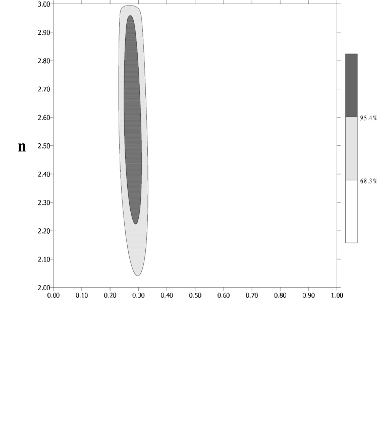
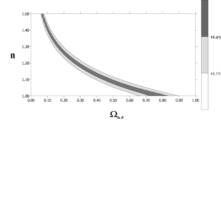
Figure 4: The comparision the the confidence levels (on the plane $(\Omega_{m,0},n)$) obtained from combined analysis SNIa Astier sample and baryon oscillations peak (upper panel) and from (CMB) ”shift parameter“ (lower panel) .

4 Flat rotation curves from cosmology in ${\cal L}\propto R^{n}$ theories

Let us consider low energy limit of modified gravity with lagrangian ${\cal L}\propto R^{n}$. For this aims it is useful to consider point like $m$ in Schwarzchild - like metric (spherically symmetric). Then modified gravitational potential which corrected the ordinary Newtonian potential is of the form:

$$V(r)\propto-\frac{1}{r}(1+(\frac{r}{r_{c}})^{\beta})$$ (16)

where $r_{c}$ is characteristic parameter which crucially depends on the mass of the system and $\beta=\beta(n)$ [43].

Hence we can evaluate the rotation curve in the Newtonian limit of modified gravity $\frac{mv_{c}^{2}(r)}{r}=-\frac{\partial V}{\partial r}$. In the previous section we estimate value of $n\simeq 2.6$. Then we calculate $\beta$ parameter from the formula:

$$\beta=\frac{12n^{2}-7n-1-\sqrt{36n^{4}+12n^{3}-83n^{2}+50n+1}}{6n^{2}+4n-2}$$ (17)

obtained by Capozzielo et al. [43].

We obtain $\beta\simeq 0.7$ which is close to $\beta$ estimated for NGC 5023 ($\beta=0.714$). Therefore we obtain that considered theory reproduce flat rotation curves of spiral galaxies. Moreover, the value of $\beta$ parameter required to explain acceleration expansion of the Universe give rise to correct peculiarities of observed rotation curve. Nevertheless note, that from investigation presented in previous section density parameter for matter is close to $\Omega_{m,0}=0.3$ rather than to value $\Omega_{m,0}=0.05$ as can be expected if both effects of dark energy and dark matter has non-substantial nature i.e. (arises from modified gravity only).

5 Conclusion

In this paper we consider the simplest choice of $f(R)$ theories with $f(R)\propto R^{n}$. The basic motivation is searching for fundamental theory of gravity capable to explain both dark energy and dark matter problems without referring to mysterious dark energy conception. For this aim we consider cosmology based on such a theory of gravity and then we use different observational constraints on independent model parameters. We consider simple flat FRW model. It is integrable in exact form after re-parametrization of time variable. From estimation based on SNIa and BOP we obtain $n>2$ which means that bouncing phase instead of big-bang singularity is generic features of such models. Because $n>2$ new $\tau$ parameter is monotonous function of cosmic time and acceleration epoch is transitional only phenomenon. In the future the universe decelerate which distinguish our model from $\Lambda$CDM one. Note that because for small value of scale factor a curvature effects are negligible in the comparison to other matter contribution, therefore, in the generic case big-bang singularity is replaced by bounce.

Analysis of SNIa Astier data shows that values of $\chi^{2}$ statistic are comparable for both $\Lambda$CDM and best fitted non-linear gravity model. For deeper analysis we use Akaike and Bayesian information criteria of model comparison and selection. We find these criteria still to favor the $\Lambda$CDM model over non-linear gravity, because (under the similar quality of the fit for both models) the $\Lambda$CDM model contains one parameter less.

Moreover, we find that the effect of dark matter can be kinematically explained as a effect of nonlinear gravity with Lagrangian ${\cal L}\propto R^{n}$. Parameter $\beta$ required for explaining accelerated expansion of the universe give rise to correct peculiarities of observed rotation curve. However from baryon oscillation peak prior we still obtain $\Omega_{m,0}\simeq 0.3$ (instead of $\Omega_{m,0}\simeq 0.05$ as we expected). Moreover, we find a disagreement between results obtained from CMB shift parameter analysis and that from joint SNIa and baryon oscillation peak. Finally, the substantial form of dark matter is still required.

References

- [1] A. G. Riess, Astron. J. 116 (1998) 1009.
- [2] S. Perlmutter, et al., Astrophys. J. 517 (1999) 565.
- [3] A. G. Riess, et al., Astrophys. J. 607 (2004) 665.
- [4] P. Astier, et al., Astron. Astrophys. 447 (2005) 31.
- [5] K. Freese, M. Lewis, Phys. Lett. B540 (2002) 1.
- [6] S. Sen, A.A Sen, Astrophys. J. 588 (2003) 1
- [7] A. Dev, J. S. Alcaniz, D. Jain (2003) astro-ph/0305068
- [8] Z.H. Zhu, M. K. Fujimoto, X.T. He, Astrophys. J. 603 (2004) 365-370
- [9] Z.H. Zhu, M. K. Fujimoto, Astrophys. J. 602 (2004) 12-17
- [10] Z.H. Zhu, M. K. Fujimoto, Astrophys. J. 585 (2003) 52-56
- [11] Z.H. Zhu, M. K. Fujimoto, Astrophys. J. 581 (2002) 1-4
- [12] W.Godlowski, M.Szydlowski, A.Krawiec, Astrophys. J 605 (2004) 599
- [13] S. Capozziello, Int. J. Mod. Phys. D 11 (2002), 483.
- [14] S.M. Carroll, V. Duvvuri, M. Trodden and M. Turner, Phys. Rev D70, (2005) 043528
- [15] S. Nojiri, S.D. Odintsov, Phys. Lett. B 576, (2003) 5 S. Nojiri, S.D. Odintsov, hep-th/0601213, S. Nojiri, S.D. Odintsov, hep-th/060808;
- [16] E.E. Flanagan, Class. Quant. Grav. 21 (2003) 417
- [17] G. Allemandi, A. Borowiec, M. Francaviglia, Phys. Rev D 70, (2004) 103503;
- [18] M.Amarzguioui, O. Elgaroy, D.F. Mota and T. Multamaki: astro-ph/0510519; T. Koivisto, D.F. Mota, Phys.Rev. D73 (2006) 083502;
- [19] O. Mena, J. Santiago, J. Weller, Phys.Rev.Lett.96 (2006) 041103;
- [20] T. Clifton, J.D. Barrow, Phys. Rev D72, (2005) 103005, T. Clifton, J.D. Barrow, Class.Quant.Grav.23 (2006) L1;
- [21] A. de la Cruz-Dombriz, A.Dobado, gr-qc/0607118;
- [22] K. Stelle, Gen. Rel. Grav. 9 (1978) 353
- [23] M. Milgrom, Astroph.J. 270 (1983) 365
- [24] S. Capozziello, V.F. Cardone, A.Troisi (2006) astro-ph/0603522
- [25] M. Persic, P. Salucci, F. Stel, Mon. Not. Roy. Astron. Soc. 281, (1996) 27; G. Gentile, P. Salucci, U. Klein, D. Vergani, P. Karbelar, Mon. Not. Roy. Astron. Soc. 351, (2004) 903.
- [26] S. Capozziello, V.F. Cardone, M.Francaviglia, Gen.Relativ.Gravit. 38 (2006) 711
- [27] A.Borowiec, W.Godlowski, M.Szydlowski, (2006) Phys. Rev D 74, (2006) 043502; astro-ph/0602526
- [28] H.J. Schmidt J.Math.Phys. 37 (1996)
- [29] A. R. Liddle, Mon. Not. Roy. Astron. Soc. 351 (2004) L49.
- [30] W. Godlowski, M. Szydlowski, Phys. Lett. B623 (2005) 10.
- [31] M. Szydlowski, W. Godlowski, Phys. Lett. B633 (2006) 427.
- [32] M. Szydlowski, W. Godlowski, A .Krawiec, J. Golbiak, Phys. Rev D 72 (2006) 063504.
- [33] H. Akaike, IEEE Trans. Auto. Control 19 (1974) 716.
- [34] G. Schwarz, Annals of Statistics 6 (1978) 461.
- [35] D. Parkinson, S. Tsujikawa, B. Basset, L.Amendola, Phys. Rev. D 71 (2005) 063524.
- [36] H. Jeffreys, Theory of Probability, 3rd Edition, Oxford University Press, Oxford, 1961.
- [37] S. Mukherjee, E. D. Feigelson, G. J. Babu, F. Murtagh, C. Fraley, A. Raftery, Astrophys. J. 508 (1998) 314.
- [38] Wang, Y. & Tegmark, M. Phys. Rev. Lett, 92, (2004) 241302.
- [39] D. N. Spergel, et al. Astrophys. J. Suppl. 148 (2003) 175.
- [40] M. Fairbairn, A. Goobar, (2005) astro-ph/0511029
- [41] D. Eisenstein et al., Astrophys. J. 633 (2005) 560.
- [42] Z. K. Guo, Z. H. Zhu, J. S. Alcaniz, Y. Z. Zhang, (2006) astro-ph/0603632
- [43] S. Capozziello, V.F. Cardone, A.Troisi, (2006) astro-ph/0602349;