The Evolution of Optical Depth in the Ly$\alpha$ Forest:
Evidence Against Reionization at $z\sim 6$

Abstract

We examine the evolution of the IGM Ly$\alpha$ optical depth distribution using the transmitted flux probability distribution function (PDF) in a sample of 63 QSOs spanning absorption redshifts $1.7<z<5.8$. The data are compared to two theoretical $\tau$ distributions: a model distribution based on the density distribution of Miralda-Escudé et al. (2000) (MHR00), and a lognormal distribution. We assume a uniform UV background and an isothermal IGM for the MHR00 model, as has been done in previous works where transmitted flux statistics have been used to infer an abrupt change in the IGM at $z\sim 6$. Under these assumptions, the MHR00 model produces poor fits to the observed flux PDFs at redshifts where the optical depth distribution is well sampled, unless large continuum corrections are applied. However, the lognormal $\tau$ distribution fits the data at all redshifts with only minor continuum adjustments. We use a simple parametrization for the evolution of the lognormal parameters to calculate the expected mean transmitted flux at $z>5.4$. The lognormal $\tau$ distribution predicts the observed Ly$\alpha$ and Ly$\beta$ effective optical depths at $z>5.7$ while simultaneously fitting the mean transmitted flux down to $z=1.6$. In contrast, the best-fitting power-law under-predicts the amount of absorption both at $z>5.7$ and at $z<2.5$. If the evolution of the lognormal distribution at $z<5$ reflects a slowly-evolving density field, temperature, and UV background, then no sudden change in the IGM at $z\sim 6$ due to late reionization appears necessary. We have used the lognormal optical depth distribution without any assumption about the underlying density field. If the MHR00 density distribution is correct, then a non-uniform UV background and/or IGM temperature may be required to produce the correct flux PDF. We find that an inverse temperature-density relation greatly improves the PDF fits, but with a large scatter in the equation of state index. The lognormal $\tau$ distribution therefore currently offers the best match to the observed flux PDF and the most reliable predictor for the transmitted flux at high redshift.

1 Introduction

The Ly$\alpha$ forest serves as our most fundamental probe of the evolution of the intergalactic medium (IGM). While numerous models have been proposed for the underlying density field (see Rauch 1998 for a review), the current consensus is a self-gravitating network of filamentary structures collapsing out of initially Gaussian density perturbations. Given a description of the IGM that relates density and transmitted flux, one can compute various cosmological parameters and examine the large-scale evolution of the Universe.

Perhaps the most dramatic inferences drawn from the evolution of Ly$\alpha$ transmitted flux is that the reionization of the IGM may have ended as late as $z\sim 6.2$ (Becker et al., 2001; White et al., 2003; Fan et al., 2002, 2006). This conclusion is based not only on the appearance of complete Gunn-Peterson troughs in the spectra of QSOs at $z>6$, but on the accelerated decline and increased variance in the mean transmitted flux at $z>5.7$ (Fan et al., 2006). Late reionization is potentially at odds with the transmitted flux seen towards the highest-redshift known QSO, SDSS J1148$+$5251 ($z_{\rm QSO}=6.42$, White et al., 2003, 2005; Oh & Furlanetto, 2005). In addition, the fact that the observed number density of Ly$\alpha$-emitting galaxies does not evolve strongly from $z\sim 5.7$ to $z\sim 6.5$ implies that the IGM is already highly ionized at these redshifts (Hu et al., 2004; Hu & Cowie, 2006; Malhotra & Rhoads, 2004, 2006; Stern et al., 2005). Galactic winds (Santos, 2004) or locally ionized bubbles (Haiman & Cen, 2005; Wyithe & Loeb, 2005; Furlanetto et al., 2004, 2006) may allow Ly$\alpha$ photons to escape even if the IGM is significantly neutral. Additional arguments may be made about the thermal history of the IGM (Theuns et al., 2002; Hui & Haiman, 2003) or the apparent size of the transmission regions around $z\sim 6$ QSOs (Mesinger & Haiman, 2004; Mesinger et al., 2004; Wyithe & Loeb, 2004; Fan et al., 2006). However, the evolution of the Ly$\alpha$ forest remains the strongest evidence for late reionization.

Still, the significance of the disappearance of transmitted flux at $z\sim 6$ has been highly debated (Songaila & Cowie, 2002; Songaila, 2004; Lidz et al., 2006a). As Songaila & Cowie (2002) pointed out, the mean transmitted flux in an inhomogeneous IGM will depend strongly on the underlying density distribution, or more precisely, on the optical depth distribution. At $z\sim 6$, any transmitted flux will arise from rare voids, which lie in the tail of the optical depth distribution. Using a sample of 19 QSOs at $z>5.7$, Fan et al. (2006) showed that the evolution the mean transmitted flux at $z\sim 6$ diverges significantly from that expected for a commonly-used model of the IGM density (Miralda-Escudé et al., 2000, referred to herein as MHR00). The question, then, is whether the MHR00 model describes the distribution of optical depths accurately enough to make reliable predictions at very high redshift.

In this paper we examine two theoretical optical depth distributions and their predictions for the Ly$\alpha$ transmitted flux probability distribution function (PDF) The first is based on the gas density distribution given by MHR00, which has been used to make claims of late reionization. Their density distribution is derived from simple arguments about the dynamics of the IGM (see §3.2) and matches the output of an earlier numerical simulation (Miralda-Escudé et al., 1996). In order to compute optical depths, assumptions must be made about the ionizing background and the thermal state of the IGM. As other authors have done, we will primarily consider a uniform UV background and an isothermal IGM. In §5 we will briefly generalize to a non-isothermal equation of state.

The second case we consider is a simple lognormal optical depth distribution. This choice can be motivated in at least two ways. Initially Gaussian density perturbations will give rise to a lognormal density field when the initial peculiar velocity field is also Gaussian (Coles & Jones, 1991). Indeed, Bi et al. (1992) demonstrated that a lognormal density distribution can produce many properties of the observed Ly$\alpha$ forest (see also Bi et al., 1995; Bi & Davidsen, 1997). More generally, however, a lognormal distribution naturally arises as a result of the central limit theorem when a quantity is determined by several multiplicative factors. For optical depth, these factors are density, temperature, and ionization rate. Here we will consider the lognormal distribution to be a generic distribution with the desirable properties of being non-zero and having a potentially large variance. Our main conclusions will not depend on any assumptions about the underlying density field.

The transmitted flux PDF has been used to constrain a variety of cosmological parameters (e.g., Rauch et al., 1997; Gaztañaga & Croft, 1999; McDonald et al., 2000; Choudhury et al., 2001; Desjacques & Nusser, 2005; Lidz et al., 2006b), with many authors assuming an optical depth distribution similar to one we consider here. We will examine the distributions themselves and their evolution with redshift by attempting to fit the models to the observed flux PDFs from a large sample of Keck HIRES data spanning Ly$\alpha$ absorption redshifts $1.7<z<5.8$. We introduce the data in §2. In §3 the optical depth distributions are derived and used to fit the observed flux PDFs. We find that the lognormal distribution provides a better fit to the data at all redshifts where the optical depth distributions are well sampled. In §4 we perform a simple fit to evolution of the lognormal distribution and use it to predict the mean transmitted flux at $z>5.7$. In §5 we modify the model distribution by applying a non-isothermal equation of state. Finally, our results are summarized in §6.

2 The Data

Observations were made using the HIRES spectrograph (Vogt et al., 1994) on Keck I between 1993 and 2006. Targets are listed in Table 1. QSOs at $z_{\rm QSO}<4.8$ were observed using the original HIRES CCD and were reduced using the MAKEE package written by Tom Barlow. QSOs at $z_{\rm QSO}>4.8$ were observed using the upgraded detector and reduced using a custom set of IDL routines as described in Becker et al. (2006). The IDL package is based on the optimal sky subtraction technique of Kelson (2003). For nearly all of our observations we used an 0$\farcs$86 slit, which gives a velocity resolution FWHM of $\Delta v=6.7$ km s^-1.

We will return to the issue of continuum fitting in §3.3. For now we will describe our baseline fitting procedure for quasars at various redshifts. For objects at $z_{\rm QSO}<4.8$, individual exposures were typically bright enough that a continuum could be fit to individual orders. This was done by hand using a slowly varying spline fit. The orders were then normalized prior to combining. At higher redshifts, we performed a relative flux calibration of each exposure using standard stars. The individual exposures were then combined prior to continuum fitting. A spline fit was again used for QSOs at $z_{\rm QSO}\leq 5.4$. However, since the transmission regions at $z>5$ rarely, if ever, reach the continuum, the fits were of a very low order and intended only to emulate the general structure of continua observed in lower redshift QSOs (e.g., Telfer et al., 2002; Suzuki, 2006). For $z_{\rm QSO}>5.7$ we used a power law fit to the continuum of the form $f_{\nu}\propto\nu^{-0.5}$.

Determining a quasar continuum is generally a subjective process whose accuracy will depend strongly on how much of the continuum has been absorbed (see Lidz et al. 2004b for a discussion). At $z\sim 3$, much of the spectrum will still be unabsorbed and errors in the continuum fit will depend on signal-to-noise of the data and the personal bias of the individual performing the fit. For high-quality data, errors in the continuum at $z\sim 3$ should be $\lesssim 1\%$. This uncertainty will increase with redshift as more of the continuum gets absorbed. By $z\sim 5.5$, very few transmission regions remain and the continuum must be inferred from the slope of the spectrum redward of the Ly$\alpha$ emission line. However, the spectral slope may have an unseen break near Ly$\alpha$. In addition, echelle data are notoriously difficult to accurately flux calibrate. We therefore expect our power-law continuum estimates at $z\sim 6$ to be off by as much as a factor of two.

3 Flux Probability Distribution Functions

3.1 Observed PDFs

Observed transmitted flux probability distribution functions (PDFs) were taken from spectra of the 63 quasars listed in Table 1. In order to avoid contamination from the proximity region and from O vi/Ly$\beta$absorption, we limited our analysis to pixels 10000 km s^-1 redward of the Ly$\alpha$ emission line and 5000 km s^-1 redward of the O vi emission line. The offsets were made intentionally large to account for possible errors in the QSO redshifts. In order for each region to contain enough pixels to be statistically significant yet avoid strong redshift evolution within a sample, we divided the Ly$\alpha$ forest in each sightline into two sections covering $\sim 60$ Å rest wavelength. Regions containing damped Ly$\alpha$ systems were discarded. We further exclude wavelengths covered by the telluric A and B bands. Other atmospheric absorption due to water vapor was typically weak compared to the Ly$\alpha$ absorption at the same wavelength and so was ignored. Table 1 lists the redshift interval for each region of the Ly$\alpha$ forest we examine.

Metal lines can be a significant contaminant in the Ly$\alpha$ forest, particularly at lower redshifts. We therefore removed as many lines as could be identified either by damped Ly$\alpha$ absorption or from multiple metal lines at the same redshift. In addition to the doublets C iv, Si iv, and Mg ii, we searched for coincidences of Si ii, Si iii, C ii, O i, Fe ii, Al ii, and Al iii. For exceptionally strong systems we also masked weaker lines such as Cr ii, Ti ii, S ii, and Zn ii. Lines in the forest were masked according to the structure and extent of lines identified redward of Ly$\alpha$ emission. Very strong line that could be identified only from their presence in the Ly$\alpha$ forest (e.g., saturated C iv) were also masked. However, we did not mask weak lines found in the forest without counterparts redward of Ly$\alpha$ emission. Doing so would preferentially discard pixels with low Ly$\alpha$ optical depth (where the metal lines can be seen), introducing a potentially larger bias in the PDF than the one incurred by leaving the contaminated pixels in the sample. In any case, our primary concern is with strong metal lines that could mimic saturated Ly$\alpha$ absorption. Weak metal lines are not expected to significantly alter the flux PDF.

The observed transmitted flux PDF for each region was computed in normalized flux bins of 0.02. Errors were computed using bootstrap resampling (Press et al., 1992). Each region was divided into many short sections spanning 200 km s^-1, and 1000 replicates of each region were constructed by randomly drawing sections with replacement. For this work we have used only the diagonal elements of the error matrix. As noted by McDonald et al. (2000) and Desjacques & Nusser (2005), ignoring the off-diagonal elements when performing $\chi^{2}$ fitting can have a significant effect on the width of the $\chi^{2}$ distribution, but has only a small effect on the values of the best-fit parameters. For comparison, we have repeated the analyses presented in this paper using purely Poisson errors and have obtained nearly identical results.

3.2 Theoretical PDFs

We will examine two possible distributions for Ly$\alpha$ optical depths: one based on the gas density distribution given by MHR00, and the other a lognormal distribution. In this section we derive the expected flux PDF for each case.

3.2.1 MHR00 model

The MHR00 gas density distribution is derived analytically based on assuming that the density fluctuations are initially Gaussian, that the gas in voids is expanding at constant velocities, and that the densities are smoothed on the Jeans length of the photoionized gas. The resulting parametric form for the volume-weighted density distribution is

$$P_{\Delta}^{\rm MHR00}(\Delta)=A\exp{\left[-\frac{(\Delta^{-2/3}-C_{0})^{2}}{2(2\delta_{0}/3)^{2}}\right]}\Delta^{-\beta}\,,$$ (1)

where $\Delta\equiv\rho/\bar{\rho}$ is the gas overdensity and $A$, $C_{0}$, $\delta_{0}$, and $\beta$ are constants. We take $\delta_{0}=7.61/(1+z)$ and $\beta$ from Table 1 of MHR00, which produces good fits to $\Lambda$CDM ($\Omega_{\rm m}=0.4$) simulation of Miralda-Escudé et al. (1996). We then set $A$ and $C_{0}$ such that the total area under $P_{\Delta}^{\rm MHR00}(\Delta)$ and the mean overdensity are both equal to one. Parameters for redshifts other than those listed in MHR00 are linearly interpolated.

To convert from densities to optical depths, assumptions must be made about the ionizing background radiation and the thermal state of the gas. The Ly$\alpha$ optical depth of a uniform IGM would be

$$\tau_{u}=\frac{\pi e^{2}}{m_{e}c}f_{\alpha}\lambda_{\alpha}H^{-1}(z)n_{{\rm H\;\mbox{\tiny I}}}\,,$$ (2)

where $f_{\alpha}$ is the Ly$\alpha$ oscillator strength, $\lambda_{\alpha}=1216$ Å, and $H(z)$ is the Hubble constant at redshift $z$ (Gunn & Peterson, 1965). In the case of photoionization equilibrium, the optical depth $\tau(\Delta)$ for an overdensity $\Delta$ can be expressed in terms of the H i ionization rate $\Gamma$, and the recombination coefficient $\alpha$ as (Weinberg et al., 1997)

$$\tau(\Delta)\propto\frac{(1+z)^{4.5}(\Omega_{\rm b}h^{2})^{2}\alpha[T(\Delta)]}{h\Gamma(\Delta,z)\Omega_{\rm m}^{0.5}}\Delta^{2}\,,$$ (3)

where $\alpha$ depends on the temperature as $\alpha(T)\propto T^{-0.7}$ for $T\sim 10^{4}$ K (Abel et al., 1997). The IGM temperature will generally depend on the density, which is typically expressed as a power-law equation of state, $T(\Delta)=T_{0}\Delta^{1-\gamma}$ (e.g., Hui & Gnedin, 1997). However, as other authors have done, we will assume a uniform UV background and an isothermal IGM (Songaila & Cowie, 2002; Songaila, 2004; Fan et al., 2002, 2006). Following Fan et al. (2002), we can then express the optical depth as a function of density,

$$\tau(\Delta)=\tau_{0}\left(\frac{1+z}{7}\right)^{4.5}\left[\frac{0.05}{\Gamma_{-12}(z)}\right]\Delta^{2}\,,$$ (4)

where $\Gamma_{-12}$ is the H i ionization rate in units of $10^{-12}~{}{\rm s}^{-1}$. For comparison to other works (McDonald & Miralda-Escudé, 2001; Fan et al., 2002, 2006), we take $\tau_{0}=82$, although the normalization depends on the choice of cosmology. Equations (1) and (4) can then be used to determine the expected distribution of optical depths,

$$P_{\tau}^{\rm MHR00}(\tau)=\frac{AG^{(\beta-1)/2}}{2\tau^{(\beta+1)/2}}\exp{\left[-\frac{\left(G^{1/3}\tau^{-1/3}-C_{0}\right)^{2}}{2(2\delta_{0}/3)^{2}}\right]}\,,$$ (5)

where

$$G\equiv\tau_{0}\left(\frac{1+z}{7}\right)^{4.5}\left[\frac{0.05}{\Gamma_{-12}(z)}\right]\,.$$ (6)

Finally, we can convert to the expected distribution of normalized fluxes, $F=e^{-\tau}$,

$$P_{F}^{\rm MHR00}(F)=\frac{AG^{(\beta-1)/2}}{2(-\ln{F})^{(\beta+1)/2}F}\exp{\left[-\frac{\left(G^{1/3}(-\ln{F})^{-1/3}-C_{0}\right)^{2}}{2(2\delta_{0}/3)}\right]}$$ (7)

for $0\leq F\leq 1$, $0$ otherwise. The distribution of fluxes at a particular $z$ is then fully specified by the ionization rate $\Gamma_{-12}$.

3.2.2 Lognormal $\tau$ distribution

For the lognormal optical depth distribution, we make no assumptions about the underlying density field, temperature, or ionization rate. As discussed above, a lognormal distribution can be motivated either from arguments about the evolution of an initially Gaussian density field (Coles & Jones, 1991; Bi et al., 1992) or by the central limit theorem. Here we consider it to be a generic model that may plausibly describe the distribution of optical depths. The lognormal distribution is described by two parameters, $\mu=\langle\ln{\tau}\rangle$, and $\sigma$, which is the standard deviation of $\ln{\tau}$,

$$P_{\tau}^{\rm Lognormal}(\tau)=\frac{1}{\tau\sigma\sqrt{2\pi}}\exp{\left[-\frac{(\ln{\tau}-\mu)^{2}}{2\sigma^{2}}\right]}\,.$$ (8)

This gives an expected distribution of transmitted fluxes,

$$P_{F}^{\rm Lognormal}(F)=\frac{1}{(-\ln{F})F\sigma\sqrt{2\pi}}\exp{\left[-\frac{(\ln{(-\ln{F})}-\mu)^{2}}{2\sigma^{2}}\right]}$$ (9)

for $0\leq F\leq 1$, $0$ otherwise. There are obvious similarities between the MHR00 and lognormal distributions, which should not be surprising if they are both expected to at least roughly describe the data. We will examine the differences between the two cases more closely in §4.1.

3.3 Fitting the observed PDFs

In order to match the observed flux PDF, we must account for various imperfections in the data. The most important of these is noise in the flux measurements, which will smooth out the PDF and create pixels with $F<0$ and $F>1$. We incorporate this effect by convolving the ideal flux PDFs given by equations (7) and (9) with a smoothing kernel constructed separately for each flux bin. (Numerically, the smoothing is performed on bins much narrower than those used for the final PDFs). The kernel for a particular bin is a weighted sum of Gaussian kernels whose widths and weights are determined from the distribution of formal flux errors of pixels in that bin. The result is typically a kernel with a narrow core to account for pixels with low noise, and an extended tail for noisier pixels. This allows us to fit regions of the Ly$\alpha$ forest where the data quality is highly inhomogeneous.

Errors in the continuum level and the flux zero point will also affect the the observed PDF. A change in the continuum will cause the observed PDF to be stretched or compressed in proportion to the flux level. An error in the zero point, which may result either from imperfect sky subtraction or from spurious counts (i.e., cosmic rays) improperly handled by the spectrum extraction or combination routines, will also stretch or compress the observed PDF from the low-flux end. In fitting the PDFs we consider two cases: first, where we assume there are no errors in either the continuum or the zero point, and second, where the continuum level and zero point are treated as free parameters. We define the preferred continuum and zero point levels to be those which, if applied to the data, would allow the theoretical distributions to produce the best. However, when performing the fits, the adjustments are applied to the models and not to the data. The continuum and zero points are treated independently, such that a change in the zero point does not require a change in the continuum, and visa versa. We do not allow zero point corrections at $z<3$, where few pixels have zero flux. This was found to have no significant impact on the other parameters.

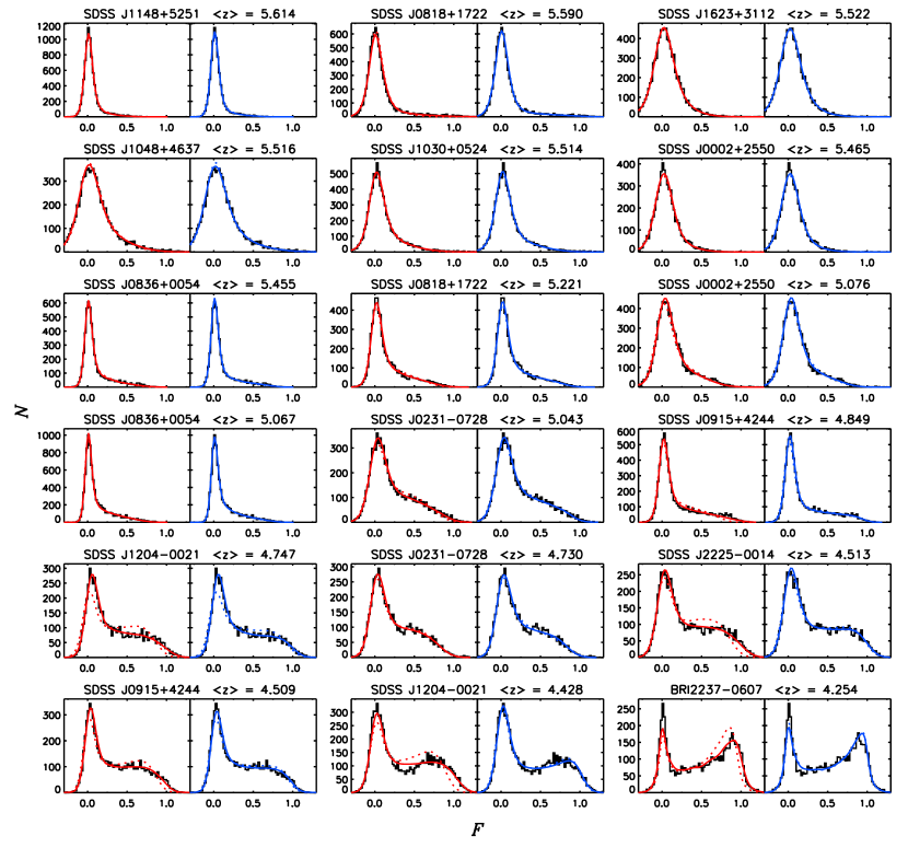
Figure 1: Fits to the Ly$\alpha$ flux probability distribution functions for QSOs in our sample. Each set of panels is labeled with the QSO name and the mean absorption redshift. Histograms show the observed PDF. For each region, MHR00 model fits assuming an isothermal IGM are shown on the left-hand side (red lines), while fits based on a lognormal $\tau$ distribution are shown on the right-hand side (blue lines). Dotted lines indicate the best fit without adjusting either the continuum or the zero point. Solid lines show the best fits when the continuum and zero point are allowed to vary. The lognormal $\tau$ distribution generally produces a good fit without large adjustments to the continuum, whereas at $3<z<5$ the MHR00 model fits tend to be poor unless a significant continuum adjustment is made.

The results of the $\chi^{2}$ minimization fitting are summarized in Tables 2 and 3 for the MHR00 and lognormal cases, respectively. The best-fitting PDFs are plotted in Figures 1 through 5. For each region, we show the observed PDF along with the best-fitting theoretical PDFs in the cases where no continuum or zero point corrections are made and where the continuum and zero point are allowed to vary. At $z>5$, the MHR00 and lognormal distribution provide very similar fits. This is not a surprise since, at these redshifts, we are sampling the low-optical depth tail of both distributions. The differences in the distributions increase at lower redshift. At $3<z<5$, the best-fit MHR00 distribution significantly under-predicts the number of pixels with very low optical depth unless a continuum correction is applied. In contrast, the best-fit lognormal distributions provide a reasonable fit to the data at all redshifts, with or without a change in the continuum. Both models under-predict the number of saturated pixels in some cases, although the discrepancy tends to be much larger for the MHR00 distribution.

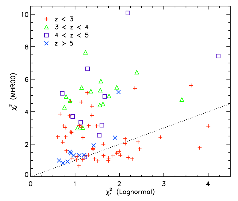
Figure 6: A comparison of the reduced $\chi^{2}$ values for the best-fitting MHR00 and lognormal $\tau$ PDFs when the continuum and zero point are held fixed. Symbols indicate the mean absorption redshift of the fitted region of the Ly$\alpha$ forest. The dotted line indicates where $\chi^{2}_{\rm r,\,MHR00}=\chi^{2}_{\rm r,\,Lognormal}$. Roughly half of the Ly$\alpha$ regions at $z<3$ are better fit by the MHR00 PDF. Otherwise, the lognormal PDF is preferred.

In Figure 6 we compare the minimum reduced $\chi^{2}$ values for both models in the case where the continua and zero points are held fixed. At $z<2$, there is a roughly even divide between regions that are better fit by the MHR00 distribution and those that prefer the lognormal distribution. However, in most instances where the MHR00 distribution is preferred, the fit is relatively poor ($\chi^{2}_{\rm r}>2$). At $z>5$, the fits are mostly comparable, as noted above. For $3<z<4$, the lognormal distribution provides a reasonable fit and is strongly preferred over the MHR00 model.

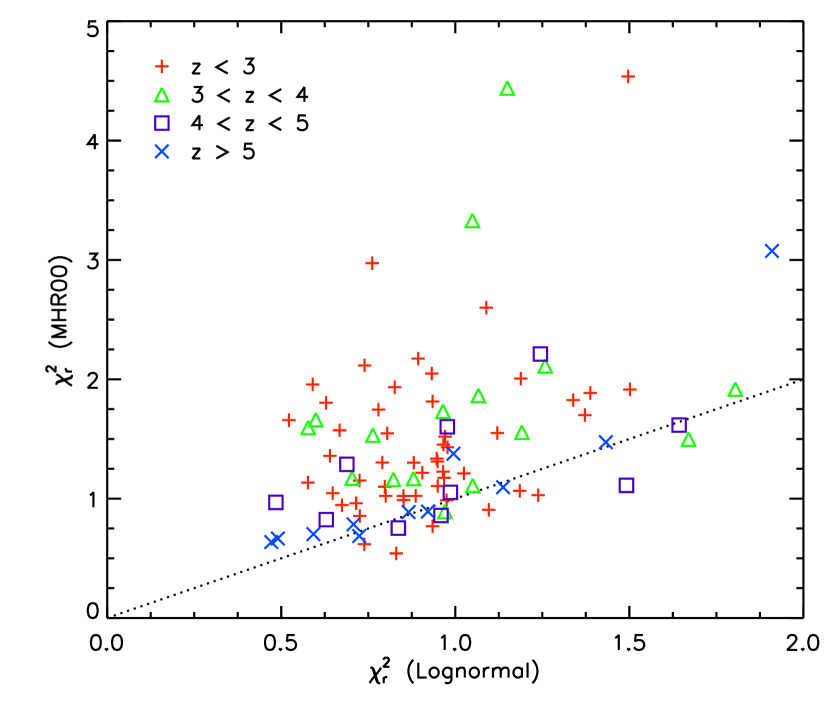
Figure 7: A comparison of the reduced $\chi^{2}$ values for the best-fitting MHR00 and lognormal $\tau$ PDFs when the continuum and zero point are allowed to vary. Note the change in scale from Figure 6. Symbols indicate the mean absorption redshift of the fitted region of the Ly$\alpha$ forest. The dotted line indicates where $\chi^{2}_{\rm r,\,MHR00}=\chi^{2}_{\rm r,\,Lognormal}$. The lognormal PDF is preferred at all redshifts, particularly at $z<5$.

The fits improve for both models when the continua and zero points are allowed to vary. Most of this improvement is the result of the continuum corrections. The effect is particularly large for the MHR00 distribution, which implies that the MHR00 model tends to require that a significant continuum correction be applied to the data in order to produce a good fit. In Figure 7 we plot the reduced $\chi^{2}$ values for these more general fits. As was the case without continuum and offset adjustments, the two distributions produce comparable fits at $z>5$. However, at all lower redshifts, the lognormal distribution is preferred.

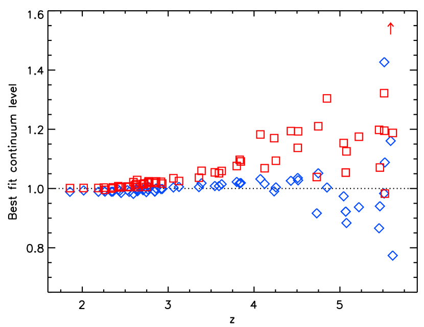
Figure 8: Continuum adjustments to the data that are required so that the observed distribution of Ly$\alpha$ fluxes are best fit by the theoretical distributions. Squares show the continuum adjustment needed for the MHR00 model. Diamonds show the continuum adjustment needed for the lognormal $\tau$ distribution. The MHR00 model value for SDSS J0818$+$1722 at $\langle z_{\rm abs}\rangle=5.590$ lies outside the plot range, as indicated by the arrow. At $z<4$, only the values for regions with median flux error $<0.05$ are shown. The MHR00 distribution requires a steadily increasing continuum adjustment with redshift to account for the lack of pixels predicted to lie near the continuum. At $z>5.4$ the best-fitting continuum has a large scatter for both distributions due to how little transmitted flux remains in the forest.

As noted above, even at low redshift, where extended regions of the spectrum have very little absorption, the continuum fit may be in error due to a combination of noise and the personal bias of the individual applying the fit. However, at $z<4$, the continuum error should be less than a few percent for reasonably high signal-to-noise data. In Figure 8 we plot the continuum correction preferred for both distributions as a function of redshift. The MHR00 model requires the continuum to steadily increase with redshift over the continuum drawn by hand in order to account for the lack of pixels predicted to lie near the continuum (i.e., pixels with very low optical depth). In contrast, the lognormal $\tau$ distribution naturally accommodates fluxes near the continuum and does not require a large continuum correction for $z<4.5$. At $z>5.4$, the preferred continuum adjustment has a large scatter for both theoretical distributions, since nearly all pixels have significant optical depth.

In Figure 9 we show examples of the best-fit continua overlaid on the corresponding regions of the Ly$\alpha$ forest. While the shape of a QSO continuum can be somewhat ambiguous when convolved with the response function of the instrument, no undue effort has been made to fit the continua across every transmission peak. The lognormal distribution fits the data well when the continua are near their intuitive values, while the MHR00 model requires the continua to be substantially higher. Fitting QSO continua is an inherently uncertain task. However, even when the continuum is allowed to vary, the lognormal $\tau$ distribution produces a better fit than the MHR00 model.

In contrast to our results, Rauch et al. (1997) and McDonald et al. (2000) found good agreement between the observed flux PDFs from some of the same sightlines used here and the predictions from a numerical simulation with a density distribution similar to the MHR00 model. The reason for this appears to lie in their treatment of the continuum. Both works apply a strong correction to their simulated spectra by placing the continuum at the maximum transmitted flux level for each pass through the simulation box (10$h^{-1}$ Mpc, or $\sim 30$ Å at $z=4$). This is a much higher-order correction than we consider here. In addition, McDonald et al. (2000) group all pixels with flux $F>1$ into their bin at $F=1$. This disguises the shape of the observed PDF for pixels with low optical depth, particularly at $z=3-4$. By fitting pixels at all fluxes, we remain sensitive to the shape of the PDF near $F\sim 1$. Applying a low-order continuum correction is therefore not sufficient to obtain a good fit for the MHR00 distribution. However, this works well in the lognormal case. Much of the discriminating power in the flux PDF occurs at very low optical depths. Therefore, unless more reliable continuum fits can be made, the success of the MHR00 model in this regime is at best unclear.

4 Redshift Evolution of Optical Depth

4.1 Lognormal Parameters

We have shown that a lognormal distribution of optical depths provides a good fit to the observed Ly$\alpha$ transmitted flux PDF at all redshifts $1.7<z<5.8$. In this section we examine the evolution of the lognormal distribution and use it to predict the evolution of the mean transmitted flux at $z>6$. In Figure 10 we plot the lognormal parameters $\mu$ and $\sigma$ as a function of $z$. Both parameters evolve smoothly with redshift, as should be expected if they reflect a slowly-evolving density field, UV background, and temperature-density relation. The increase in $\mu$ and decrease in $\sigma$ with $z$ can both be understood primarily in terms of the evolution of a self-gravitating density field. At earlier times, the density contrast in the IGM will be lower. This will tend to produce a higher volume-weighted median $\tau$, which is given by $e^{\mu}$, as well as a smaller logarithmic dispersion in $\tau$, which is given by $\sigma$. Since we do not have an a priori model for how the lognormal parameters should evolve, for this work we choose the simplest possible parametrization. Excluding points at $z>5.4$, where the lognormal parameters depend on highly uncertain continuum levels, a linear fit in redshift gives

$$\mu(z)=(-9.35\pm 0.17)+(1.79\pm 0.04)(1+z)\,,$$ (10)

$$\sigma(z)=(4.19\pm 0.16)-(0.46\pm 0.03)(1+z)\,.$$ (11)

These fits are plotted as dashed lines in Figure 10.

We can compare the evolution of the MHR00 and lognormal $\tau$ distributions and their predictions for the transmitted flux PDF. In Figure 11 we plot fiducial $\tau$ and flux distributions for $2\leq z\leq 6$. Parameters for the lognormal distribution are calculated from equations (10) and (11). For the MHR00 model, values for $\Gamma_{-12}$ are chosen to be consistent with the fitted values in Table 2. The vertical dotted lines indicate the range of optical depths that can be measured with good data. At $z=2$ we are primarily sensitive to the high-$\tau$ tail in both distributions. At higher redshifts, the peaks of the distributions shift towards higher values of $\tau$ until we are sampling only the end of the low-$\tau$ tail at $z=6$.

Differences in the shape of the transmitted flux PDF are largest at $3\leq z\leq 5$, where $P_{\tau}(\tau)$ is well-sampled. The fact that the lognormal $\tau$ distribution is most strongly favored at these redshifts suggests that it is more likely to be useful in making predictions for the distribution of transmitted flux at $z>6$. An important feature of the lognormal distribution is that it narrows with redshift more rapidly than the MHR00 distribution. It therefore predicts fewer pixels with measurable transmitted flux at $z\sim 6$ than does the MHR00 model with a slowly evolving UV background.

4.2 Mean transmitted flux

We can use the redshift evolution of the lognormal distribution to predict the the evolution of transmitted flux at $z\gtrsim 6$. The mean transmitted flux will be given by

$$\langle F\rangle=\int_{0}^{1}F\,P_{F}(F)\,dF\,.$$ (12)

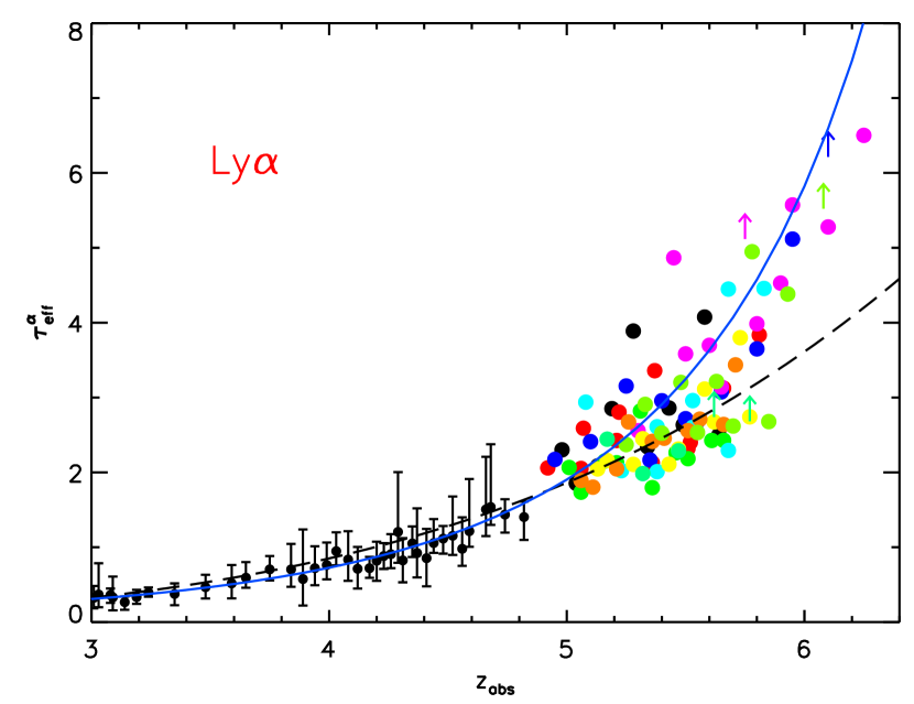
Figure 12: The evolution of Ly$\alpha$ effective optical depth with redshift, where $\tau_{\rm eff}=-\ln{\langle F\rangle}$. Data points are from Songaila (2004) (small circles) and Fan et al. (2006) (large circles and arrows, with colors matching their Figure 2). The dashed line shows the best-fit power-law to $\tau_{\rm eff}^{\alpha}$ at $z<5.5$ from Fan et al. (2006). The solid line shows $\tau_{\rm eff}^{\alpha}$ calculated from the lognormal distribution of Ly$\alpha$ optical depths, for which the parameters were fit at $z<5.4$. A simple evolution in the lognormal $\tau$ distribution predicts the upturn in $\tau_{\rm eff}^{\alpha}$ at $z>5.5$ and produces a better fit to the observed $\tau_{\rm eff}^{\alpha}$ at $4<z<5$.

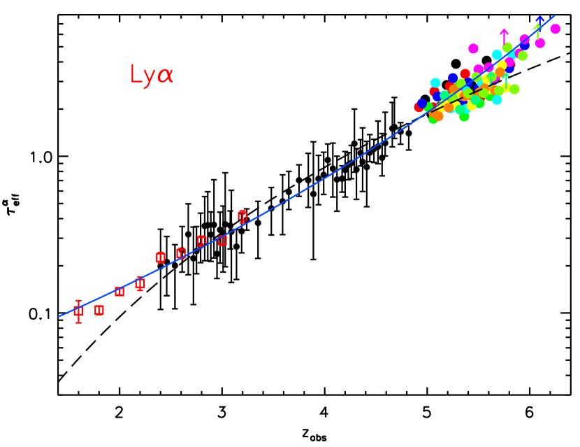
Figure 13: Same as Figure 12, with $\tau_{\rm eff}^{\alpha}$ on a logarithmic scale. We have also included lower-redshift measurements calculated from Kirkman et al. (2005), which exclude absorption from metal lines, Lyman limit systems, and damped Ly$\alpha$ systems. The Kirkman et al. (2005) points are plotted as open squares with errors in the mean measurements. The power-law fit from Fan et al. (2006) (dashed line) under-predicts the amount of Ly$\alpha$ absorption both at $z>5.7$ and at $z<2.5$. In contrast, $\tau_{\rm eff}^{\alpha}$ calculated from the lognormal $\tau$ distribution (solid line), provides a simultaneously good fit to all points at $1.6<z<6.2$.

It is conventional to express the mean flux in terms of an effective optical depth $\tau_{\rm eff}=-\ln{\langle F\rangle}$. For a distribution of optical depths, $\tau_{\rm eff}$ will be smaller than the true mean optical depth. We show measurements of $\tau_{\rm eff}$ for Ly$\alpha$ from Songaila (2004) and Fan et al. (2006) in Figure 12. The dashed line shows the best-fitting power-law to their data at $z<5.5$ from Fan et al. (2006). The deviation of the data from the power-law at $z>5.7$ has been cited as the primary evidence for an abrupt change in the ionizing background at $z\sim 6$. We also show $\tau_{\rm eff}^{\alpha}$ as predicted by the evolution of the lognormal $\tau$ distribution given by equations (10) and (11) as a solid line. We emphasize that the lognormal parameters were fit only to measurements at $z<5.4$. Even so, $\tau_{\rm eff}^{\alpha}$ calculated from the lognormal distribution both better fits the data at $z<5$ and predicts the upturn in $\tau_{\rm eff}^{\alpha}$ at $z>5.7$. In Figure 13 we include the lower-redshift measurements of Kirkman et al. (2005). The power-law under-predicts the amount of Ly$\alpha$ absorption at $z<2.5$, while the lognormal distribution matches all observations at $1.6<z<6.2$.

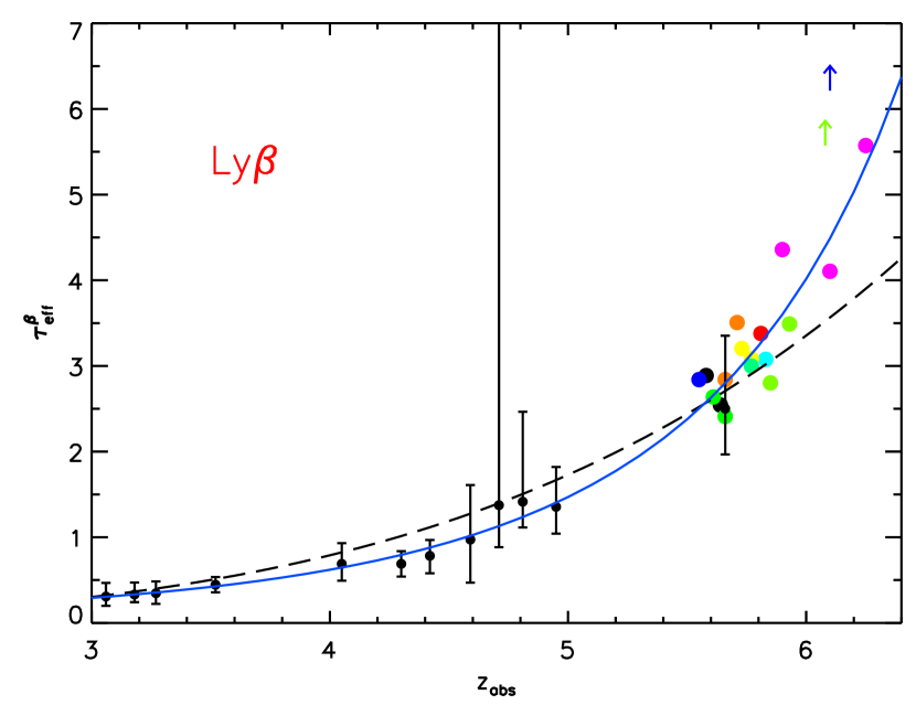
Figure 14: The evolution of Ly$\beta$ effective optical depths with redshift. Data points at from Songaila (2004) (small circles) and Fan et al. (2006) (large circles and arrows, with colors matching their Figure 3). The data have not been corrected for foreground Ly$\alpha$ absorption. The dashed line shows the best-fit power-law to $\tau_{\rm eff}^{\beta}$ at $z<5.5$ from Fan et al. (2006). The solid line shows $\tau_{\rm eff}^{\beta}$ predicted purely from the lognormal distribution of Ly$\alpha$ optical depths. Even though no independent fitting of Ly$\beta$ fluxes was performed, the lognormal $\tau$ distribution captures the upturn in $\tau_{\rm eff}^{\beta}$ at $z>5.5$ and produces a better fit to the observed $\tau_{\rm eff}^{\beta}$ at $4<z<5$.

Stronger constraints on the ionization state of the IGM can be set using Ly$\beta$, which is a weaker transition than Ly$\alpha$ by a factor of 6.2. In the lognormal case, this produces a distribution of Ly$\beta$ optical depths with the same $\sigma$ as Ly$\alpha$ but with $\mu_{\beta}=\mu_{\alpha}-\ln{6.2}$. We can then compute the expected mean flux in the Ly$\beta$ forest at redshift $z$ by multiplying the mean transmission resulting from Ly$\beta$ absorption at $z$ by the mean transmission resulting from Ly$\alpha$ absorption at $z_{\beta}=(1+z)\lambda_{\beta}/\lambda_{\alpha}-1$. We show the $\tau_{\rm eff}^{\beta}$ measurements from Songaila (2004) and Fan et al. (2006) in Figure 14. These are computed directly from the transmitted flux and have not been corrected for foreground Ly$\alpha$ absorption. The dashed line again shows the best-fit power-law to the points at $z<5.5$ from Fan et al. (2006). The solid line shows the lognormal prediction. Here again, despite the fact that we have not used any Ly$\beta$ measurements to determine the optical depth distribution, $\tau_{\rm eff}^{\beta}$ predicted in the lognormal case is a better fit to the data at $z<5$ and follows the upturn in $\tau_{\rm eff}^{\beta}$ at $z>5.7$.

Our purpose here is not to fully characterize the evolution of transmitted flux at all redshifts. We have simply identified a distribution of optical depths that describes the observed distribution of transmitted fluxes better than the commonly used model. The fact that this distribution evolves smoothly with redshift, and that the same evolution describes changes in the Ly$\alpha$ forest as well at $z\sim 6$ as it does at $z\sim 3$ strongly suggests that the disappearance of transmitted flux at $z>6$ is due to a smooth evolution of IGM properties. The lognormal prediction for $\tau_{\rm eff}^{\beta}$ falls slightly below some of the lower limits of Fan et al. (2006) at $z\sim 6$, but the prediction does not take into account the expected scatter in the mean flux or any small deviation from our adopted linear redshift evolution of the lognormal parameters. The important point is that the evolution of the mean transmitted flux can be well described by a smooth evolution in the underlying optical depths. When sampling only the tail of the $\tau$ distribution, as at $z\sim 6$, a slight change in the optical depths will produce a large change in the transmitted flux.

4.3 UV background

Liu et al. (2006) recently demonstrated that a semi-analytic model based on a lognormal density distribution can reproduce the observed rise in $\tau_{\rm eff}$ at $z>5.7$. However, they invoke a UV background that declines rapidly with redshift, decreasing by a factor of $\sim 11$ from $z=3$ to $5$, and by a factor of $\sim 7$ from $z=5$ to $6$. We have not assumed that the lognormal $\tau$ distribution used here arises directly from a lognormal density distribution. However, if we assume a uniform UV background and an isothermal IGM, than we can calculate the H i ionization rate by inverting equation (4) and averaging over all densities. Doing so gives

$$\Gamma_{-12}=0.05\left(\frac{1+z}{7}\right)^{4.5}\frac{\tau_{0}}{\langle\tau^{1/2}\rangle^{2}}\,,$$ (13)

where $\langle\tau^{1/2}\rangle^{2}=e^{\mu+\sigma^{2}/4}$, and we have used the fact that $\langle\Delta\rangle=1$.

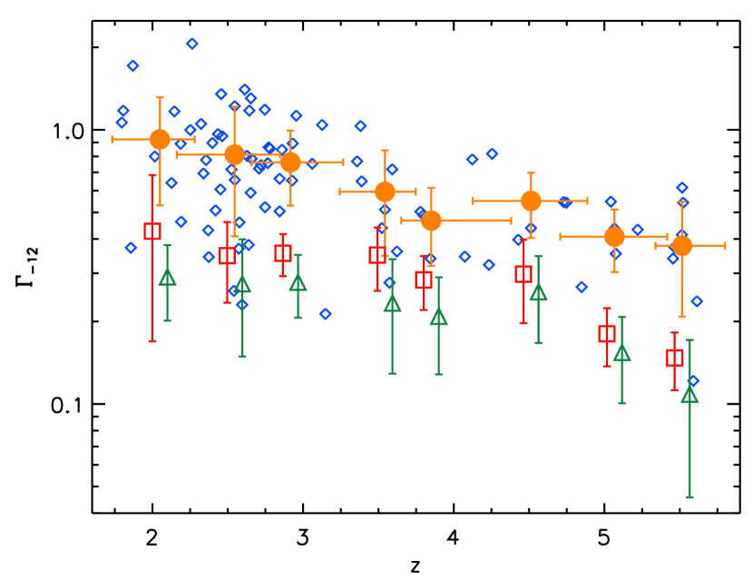
Figure 15: H i ionization rate as a function of redshift. Small diamonds show $\Gamma_{-12}$ calculated from the lognormal fits to individual regions, assuming a uniform UV background (cf. equation 13). Points fit to high-$S/N$ data are shown in blue. Filled circles show the mean $\Gamma_{-12}$ for the lognormal model in redshift bins of 0.5, starting at $z=2$. Vertical error bars show the standard deviation of points within a bin. Horizontal error bars show the range of redshift covered by all points within that bin. Squares show the mean $\Gamma_{-12}$ from the MHR00 model fits for an isothermal IGM and uniform UV background ($\alpha=0$). Triangles show the mean $\Gamma_{-12}$ from the MHR00 model fits when $\alpha$ is allowed to vary.

In Figure 15 we show $\Gamma_{-12}$ calculated for each fitted region along with the mean values in bins of redshift. For comparison, the best-fit values of $\Gamma_{-12}$ for the model distribution are also shown. The lognormal values are somewhat higher than the model values, which are in turn roughly consistent with previous measurements (McDonald & Miralda-Escudé, 2001; Fan et al., 2006). However, we do not require the strong evolution in $\Gamma_{-12}$ given by Liu et al. (2006) for the lognormal model. Transforming from densities to optical depths depends on a number of factors, and we do not presume that the assumptions implicit in equation (13) are valid. We merely point out that a lognormal $\tau$ distribution is consistent with a slowly evolving UV background.

We can also calculate the mean volume-weighted neutral fraction,

$$f_{{\rm H\;\mbox{\tiny I}}}=(5.5\times 10^{-5})\,h_{70}^{-1}\left(\frac{\Omega_{\rm m}}{0.3}\right)^{1/2}\left(\frac{\Omega_{\rm b}}{0.04}\right)^{-1}(1+z)^{-3/2}\langle\tau\rangle\,,$$ (14)

where we have used $H(z)\approx H_{0}\Omega_{\rm m}^{1/2}(1+z)^{3/2}$. The mean optical depth for the lognormal distribution will be $\langle\tau\rangle=e^{\mu+\sigma^{2}/2}$. Calculating $\mu$ and $\sigma$ from equations (10) and (11), this gives $f_{{\rm H\;\mbox{\tiny I}}}=[1.0,1.2,1.9,4.0,11,20]\times 10^{-5}$ for $z=[2,3,4,5,6,6.5]$. The mean optical depth will depend strongly on the high-$\tau$ tail of the distribution, which is poorly constrained at $z>4$. However, the disappearance of transmitted flux at $z>6$ is at least consistent with a highly-ionized IGM.

5 An inverse temperature-density relation?

We have shown that the simplest transformation of the MHR00 gas density distribution to optical depths provides at best an uncertain fit to the observed distribution of transmitted fluxes. However, there are several ways to modify the expected $\tau$ distribution. Here we consider a non-isothermal temperature-density relation. From equation (3) we have $\tau\propto T^{-0.7}\Gamma^{-1}\Delta^{2}$. We will address the general case where either $T$ or $\Gamma$ may depend on $\Delta$. For a power law $T^{0.7}\Gamma\propto\Delta^{\alpha}$, this gives

$$\tau(\Delta)=\tau_{0}\left(\frac{1+z}{7}\right)^{4.5}\left[\frac{0.05}{\Gamma_{-12}(z)}\right]\Delta^{2-\alpha}\,,$$ (15)

where $\Gamma_{-12}$ is now the H i ionization rate at the mean density, and the temperature at the mean density is included in $\tau_{0}$. For a uniform UV background, the equation of state index will be $\gamma=1+1.43\alpha$.

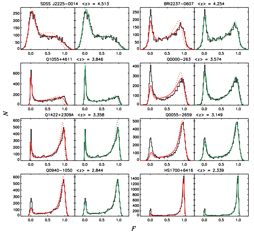
Figure 16: Examples of transmitted flux PDFs where the MHR00 model fit is significantly improved by allowing a non-isothermal temperature-density relation, or more generally, $T^{0.7}\Gamma\propto\Delta^{\alpha}$. Each set of panels is labeled with the QSO name and the mean absorption redshift. Histograms show the observed PDF. For each section, MHR00 model fits with $\alpha=0$ are shown on the left-hand side (red lines), while fits with $\alpha$ treated as a free parameter are shown on the right-hand side (green lines). Dotted lines indicate the best fit without adjusting either the continuum or the zero point. Solid lines show the best fits when the continuum and zero point are allowed to vary. The mean value of $\alpha$ for all regions is $\langle\alpha\rangle\approx-0.4$. This may indicate that the UV background decreases with density, or that there exists an inverse temperature-density relation. Alternatively, finding $\alpha<0$ may be an artifact of some other features of the MHR00 model that causes it to disagree with the data.

Not surprisingly, adding a degree of freedom significantly improves the fits for many of our Ly$\alpha$ forest regions. The fitting results are summarized in Table 4, and a sample of the fits are shown in Figure 16. There is a large scatter in the best-fit $\alpha$ at all redshifts when the continuum and zero point are allowed to vary. However, the mean value $\langle\alpha\rangle=-0.36\pm 0.45$ (sample variance) suggests that $T^{0.7}\Gamma$ increases towards lower densities. For a uniform UV background, this implies an equation of state $T(\Delta)\propto\Delta^{\gamma-1}$ with $\gamma\approx 0.5$. An index $<1$ disagrees with previous measurements using the flux PDF (Choudhury et al., 2001; Lidz et al., 2006b; Desjacques & Nusser, 2005). However, those works typically considered only $\gamma>1$, which is expected following reionization if overdense regions experience more photoionization heating and less adiabatic cooling than underdense regions. Radiative transfer effects may create a complex temperature-density relation if underdense regions are reionized by a harder UV background than the dense regions near ionizing sources (Bolton et al., 2004). For the flux PDF, $\gamma<1$ allows for a lower $\Gamma$ (typically by $\sim 20$%, see Figure 15), creating more saturated pixels, while at the same time maintaining a low $\tau$ in low density regions. The necessary continuum corrections also decrease, although they are still roughly half of those needed in the case of $\alpha=0$. Of course, it is possible that we are not measuring the real equation of state, and that the added degree of freedom simply compensates for some other aspect of the model distribution. A more careful treatment of this problem will be reserved for future work.

6 Conclusions

We have analyzed the Ly$\alpha$ transmitted flux probability distribution in a high-resolution sample of 63 QSOs spanning the absorption redshift range $1.7<z<5.8$. Our main goal has been to assess how well the theoretical optical depth distribution commonly used to measure the H i ionization rate describes the observed flux PDF. We find that the MHR00 model, under the assumptions of a uniform UV background and an isothermal IGM, produces a poor fit to the observed flux PDF at all redshifts where the optical depth distribution is well sampled. This discrepancy eases only if large continuum corrections are applied.

In contrast, a lognormal distribution of optical depths fits the data well with only minor continuum adjustments. The parameters of the lognormal distribution evolve smoothly with redshift, as expected for a slowly evolving IGM, and reflect both an increase in the mean $\tau$ and a decrease in the relative scatter in $\tau$ with redshift. We have performed simple linear fits to the lognormal parameters at $z<5.4$. The mean transmitted flux calculated from these fits matches the observations at $1.6<z<5.7$ better than the best-fitting power law (Fan et al., 2006). In addition, extrapolating the lognormal evolution to $z>6$ predicts the observed upturn in both Ly$\alpha$ and Ly$\beta$ effective optical depths. This strongly suggests that if a slowly evolving density field, ionizing background, and IGM temperature are responsible for the evolution of the Ly$\alpha$ forest at $z<5$, then there is no reason to suspect a sudden change in the IGM at $z\sim 6$.

We emphasize that we have used the lognormal distribution as a phenomenological description of the optical depths only, and that the distribution may not hold for optical depths that are outside the dynamic range of the transmitted flux. Other factors, such a non-isothermal IGM or variations in the UV background are likely to be important in deriving the optical depth distribution from the underlying density field. We have explored the possibility of a non-isothermal IGM in the context of the MHR00 model. The best fits tend to favor an inverse temperature-density relation, where temperature increases with density. This is contrary to typical expectations for the balance between photoionization heating and adiabatic cooling (Hui & Gnedin, 1997), and may be an artifact of some other feature that causes the MHR00 model to disagree with the data. However, as Bolton et al. (2004) point out, radiative transfer effects may create a complex thermodynamic state in the IGM. If gas at a given density can have a range of temperatures and/or ionization rates, then a MHR00-like density distribution may give rise to a $\tau$ distribution that is closer to lognormal.

The largest source of uncertainty in fitting the flux PDFs remains the continuum level. Much of the disagreement between the MHR00 model and observed PDFs stems from the lack of pixels predicted to have very low optical depths at $z>3$. This can be at least partially remedied by adjusting the continuum (see also McDonald et al., 2000). However, a dramatic change in the IGM would still be required to explain the observed lack of transmitted flux at $z\sim 6.2$ (e.g., Fan et al., 2002, 2006). Future observation of $z>4$ gamma-ray bursts, whose continuum is a simple power law, may help to establish the correct flux PDF. For now, we have identified an optical depth distribution that both fits the data down to $z=1.6$ and captures the evolution of the mean transmitted flux at $z>5.7$. If the lognormal distribution truly reflects aspects of the real optical depth distribution, then the motivation for late reionization may be greatly diminished.

Table 1: Fitted Ly$\alpha$ Forest Regions

QSO	$z_{\rm QSO}$	$\langle z_{\rm abs}\rangle$	$z_{\rm abs}^{\rm min}$	$z_{\rm abs}^{\rm max}$	median flux error
SDSS J1148$+$5251	6.42	5.614	5.430	5.802	0.05
SDSS J1030$+$0524	6.30	5.514	5.339	5.692	0.11
SDSS J1623$+$3112	6.25	5.522	5.339	5.709	0.15
SDSS J1048$+$4637	6.23	5.516	5.339	5.696	0.15
SDSS J0818$+$1722	6.00	5.590	5.417	5.766	0.10
		5.221	5.066	5.417	0.07
SDSS J0002$+$2550	5.82	5.465	5.339	5.592	0.12
		5.076	4.910	5.245	0.11
SDSS J0836$+$0054	5.80	5.455	5.339	5.573	0.05
		5.067	4.893	5.245	0.04
SDSS J0231$-$0728	5.42	5.043	4.885	5.206	0.11
		4.730	4.563	4.885	0.09
SDSS J0915$+$4244	5.20	4.849	4.707	4.993	0.07
		4.509	4.373	4.647	0.07
SDSS J1204$-$0021	5.09	4.747	4.582	4.887	0.09
		4.428	4.277	4.582	0.09
SDSS J2225$-$0014	4.87	4.513	4.381	4.647	0.10
		4.234	4.087	4.381	0.11
BRI1202$-$0725	4.69	4.074	3.929	4.214	0.10
BRI2237$-$0607	4.56	4.254	4.126	4.377	0.07
Q0246$+$1750	4.44	4.123	3.988	4.260	0.05
		3.851	3.716	3.988	0.07
Q1055$+$4611	4.15	3.846	3.719	3.975	0.02
		3.591	3.460	3.719	0.03
Q0000$-$263	4.13	3.833	3.704	3.961	0.05
		3.574	3.447	3.704	0.05
Q1645$+$5520	4.10	3.798	3.672	3.927	0.01
		3.543	3.417	3.672	0.02
BRI0241$-$0146	4.08	3.779	3.652	3.906	0.05
		3.523	3.398	3.652	0.06
Q0827$+$5255	3.91	3.623	3.503	3.748	0.01
		3.389	3.265	3.503	0.02
Q0055$-$2659	3.65	3.381	3.266	3.499	0.05
		3.149	3.033	3.266	0.06
Q1422$+$2309A	3.63	3.358	3.243	3.475	0.02
		3.126	3.011	3.243	0.02
Q0930$+$2858	3.44	2.955	2.845	3.067	0.07
Q0642$+$44	3.40	2.927	2.818	3.037	0.08
Q0956$+$1217	3.31	3.061	2.954	3.169	0.04
		2.845	2.738	2.954	0.05
HS0741$+$4741	3.23	2.772	2.664	2.876	0.03
Q0636$+$6801	3.18	2.931	2.827	3.036	0.02
		2.720	2.618	2.827	0.02
Q1140$+$3508	3.16	2.916	2.813	3.021	0.03
		2.708	2.605	2.813	0.03
HS1011$+$4315	3.14	2.766	2.657	2.869	0.04
Q0449$-$1326	3.10	2.860	2.757	2.962	0.04
		2.654	2.552	2.757	0.07
Q0940$-$1050	3.08	2.844	2.743	2.947	0.04
		2.639	2.538	2.743	0.05
HS1946$+$7658	3.07	2.627	2.524	2.728	0.03
Q2231$-$0015	3.02	2.780	2.680	2.881	0.05
		2.578	2.479	2.680	0.07
Q1107$+$487	2.98	2.546	2.446	2.646	0.04
Q1437$+$3007	2.98	2.547	2.448	2.648	0.05
Q0216$+$0803	2.98	2.574	2.487	2.658	0.15
Q1437$+$3007	2.98	2.746	2.648	2.846	0.04
Q0216$+$0803	2.98	2.748	2.659	2.843	0.12
Q1244$+$3133	2.97	2.541	2.439	2.638	0.10
Q1511$+$0907	2.89	2.658	2.562	2.756	0.06
		2.464	2.368	2.562	0.08
Q1132$+$2243	2.88	2.652	2.556	2.750	0.06
		2.456	2.361	2.556	0.09
HS0119$+$1432	2.87	2.643	2.547	2.740	0.03
		2.452	2.353	2.547	0.04
Q1549$+$1919	2.84	2.613	2.517	2.707	0.01
		2.419	2.324	2.517	0.01
Q0528$-$250	2.81	2.595	2.492	2.683	0.05
		2.398	2.302	2.492	0.07
Q2344$+$1228	2.79	2.374	2.280	2.470	0.09
HS1700$+$6416	2.74	2.525	2.432	2.619	0.01
		2.339	2.244	2.432	0.02
Q1442$+$2931	2.66	2.264	2.169	2.352	0.03
Q1009$+$2956	2.65	2.436	2.345	2.527	0.02
		2.252	2.162	2.343	0.02
Q1358$+$1134	2.58	2.370	2.282	2.461	0.15
Q2343$+$1232	2.58	2.190	2.101	2.281	0.10
Q2206$-$199N	2.57	2.356	2.269	2.447	0.03
		2.188	2.105	2.269	0.04
Q1623$+$2653	2.53	2.323	2.235	2.411	0.06
		2.146	2.058	2.235	0.10
Q0841$+$1256	2.51	2.127	2.038	2.214	0.12
Q0237$-$233	2.24	2.050	1.966	2.128	0.06
Q1225$+$3145	2.21	2.016	1.938	2.098	0.03
		1.857	1.777	1.938	0.04
Q0421$+$019	2.05	1.870	1.795	1.947	0.08
Q0119$-$0437	1.98	1.807	1.733	1.876	0.14
Q0058$+$0155	1.96	1.797	1.734	1.859	0.12

Table 2: Best-Fit MHR00 Model Parameters (Isothermal)

QSO	$\langle z_{\rm abs}\rangle$	$N_{\rm bin}$	Continuum and zero point fixed			Continuum and zero point allowed to vary
			$\Gamma_{-12}$	$\chi^{2}_{r}$		$\Gamma_{-12}$	Cont.	zero point	$\chi^{2}_{r}$
SDSS J1148$+$5251	5.614	49	0.14	1.32		0.12	1.188	0.005	0.67
SDSS J0818$+$1722	5.590	83	0.14	5.21		0.11	2.427	0.000	3.08
SDSS J1623$+$3112	5.522	76	0.15	0.93		0.14	0.983	0.005	0.89
SDSS J1048$+$4637	5.516	88	0.22	1.93		0.20	1.195	-0.006	1.38
SDSS J1030$+$0524	5.514	83	0.21	1.30		0.17	1.322	0.006	0.89
SDSS J0002$+$2550	5.465	68	0.13	1.34		0.12	1.071	0.009	1.10
SDSS J0836$+$0054	5.455	55	0.20	1.00		0.18	1.198	0.002	0.64
SDSS J0818$+$1722	5.221	73	0.23	1.53		0.20	1.175	0.006	0.78
SDSS J0002$+$2550	5.076	75	0.17	2.40		0.14	1.125	0.016	1.47
SDSS J0836$+$0054	5.067	56	0.16	0.84		0.16	1.054	0.003	0.70
SDSS J0231$-$0728	5.043	78	0.30	1.43		0.25	1.153	0.012	0.69
SDSS J0915$+$4244	4.849	71	0.19	3.35		0.16	1.304	0.007	0.97
SDSS J1204$-$0021	4.747	75	0.40	7.42		0.27	1.210	0.031	1.05
SDSS J0231$-$0728	4.730	77	0.27	1.22		0.25	1.039	0.012	0.86
SDSS J2225$-$0014	4.513	80	0.30	3.70		0.24	1.193	0.010	0.82
SDSS J0915$+$4244	4.509	77	0.33	3.17		0.26	1.137	0.017	0.75
SDSS J1204$-$0021	4.428	79	0.36	6.64		0.28	1.194	0.005	1.60
BRI2237$-$0607	4.254	84	0.64	4.94		0.50	1.094	-0.005	1.62
SDSS J2225$-$0014	4.234	86	0.28	5.13		0.21	1.170	-0.002	1.29
Q0246$+$1750	4.123	65	0.40	2.55		0.34	1.069	0.009	1.11
BRI1202$-$0725	4.074	87	0.29	10.08		0.23	1.182	0.011	2.21
Q0246$+$1750	3.851	78	0.55	5.26		0.39	1.073	-0.005	2.11
Q1055$+$4611	3.846	62	0.24	4.68		0.22	1.091	0.002	1.60
Q0000$-$263	3.833	70	0.34	5.50		0.28	1.097	0.010	1.56
Q1645$+$5520	3.798	60	0.33	5.49		0.31	1.076	0.002	1.53
BRI0241$-$0146	3.779	67	0.40	6.43		0.29	1.076	0.019	1.86
Q0827$+$5255	3.623	55	0.31	4.93		0.32	1.059	0.000	1.66
Q1055$+$4611	3.591	63	0.51	7.66		0.41	1.052	0.004	1.73
Q0000$-$263	3.574	73	0.44	5.32		0.32	1.048	0.002	3.33
Q1645$+$5520	3.543	61	0.33	4.27		0.28	1.055	0.000	1.17
BRI0241$-$0146	3.523	74	0.32	4.96		0.26	1.064	0.000	1.92
Q0827$+$5255	3.389	61	0.33	5.88		0.27	1.060	0.004	1.17
Q0055$-$2659	3.381	67	0.69	3.02		0.51	1.030	0.010	1.11
Q1422$+$2309A	3.358	58	0.56	4.41		0.42	1.037	0.008	1.16
Q0055$-$2659	3.149	73	0.54	4.75		0.44	1.014	0.013	4.44
Q1422$+$2309A	3.126	57	0.44	2.99		0.37	1.025	0.004	0.89
Q0956$+$1217	3.061	64	0.37	4.47		0.29	1.035	0.001	1.50
Q0930$+$2858	2.955	74	0.49	1.24		0.44	1.011	$\cdots$	1.02
Q0636$+$6801	2.931	56	0.50	3.02		0.39	1.017	$\cdots$	1.30
Q0642$+$44	2.927	76	0.38	2.12		0.29	1.030	$\cdots$	0.95
Q1140$+$3508	2.916	60	0.58	4.64		0.39	1.023	$\cdots$	2.05
Q0449$-$1326	2.860	65	0.38	1.60		0.30	1.024	$\cdots$	0.54
Q0956$+$1217	2.845	66	0.62	3.04		0.45	1.018	$\cdots$	1.75
Q0940$-$1050	2.844	61	0.39	3.14		0.30	1.019	$\cdots$	1.81
Q2231$-$0015	2.780	64	0.37	3.12		0.30	1.021	$\cdots$	1.92
HS0741$+$4741	2.772	60	0.49	4.59		0.35	1.024	$\cdots$	1.45
HS1011$+$4315	2.766	63	0.44	2.46		0.32	1.019	$\cdots$	1.13
Q0216$+$0803	2.748	86	0.21	1.30		0.19	1.010	$\cdots$	1.23
Q1437$+$3007	2.746	65	0.49	1.14		0.45	1.005	$\cdots$	1.03
Q0636$+$6801	2.720	56	0.35	2.75		0.27	1.017	$\cdots$	1.22
Q1140$+$3508	2.708	61	0.56	3.12		0.40	1.014	$\cdots$	1.66
Q1511$+$0907	2.658	70	0.42	1.74		0.35	1.011	$\cdots$	1.34
Q0449$-$1326	2.654	69	0.39	1.18		0.45	0.990	$\cdots$	0.91
Q1132$+$2243	2.652	71	0.39	2.72		0.27	1.022	$\cdots$	1.55
HS0119$+$1432	2.643	58	0.54	1.34		0.48	1.005	$\cdots$	1.15
Q0940$-$1050	2.639	66	0.38	3.85		0.24	1.029	$\cdots$	1.80
HS1946$+$7658	2.627	59	0.36	2.45		0.28	1.015	$\cdots$	1.10
Q1549$+$1919	2.613	53	0.50	3.14		0.43	1.011	$\cdots$	1.17
Q0528$-$250	2.595	65	0.25	5.44		0.16	1.022	$\cdots$	4.54
Q2231$-$0015	2.578	74	0.29	1.56		0.26	1.007	$\cdots$	1.52
Q0216$+$0803	2.574	89	0.18	1.32		0.19	0.991	$\cdots$	1.31
Q1437$+$3007	2.547	73	0.45	1.44		0.41	1.005	$\cdots$	1.43
Q1107$+$487	2.546	72	0.55	1.05		0.49	1.005	$\cdots$	0.96
Q1244$+$3133	2.541	81	0.22	2.34		0.20	1.011	$\cdots$	2.12
HS1700$+$6416	2.525	54	0.57	2.41		0.44	1.007	$\cdots$	1.57
Q1511$+$0907	2.464	76	0.31	1.03		0.30	1.002	$\cdots$	1.02
Q1132$+$2243	2.456	74	0.43	1.28		0.48	0.994	$\cdots$	1.21
HS0119$+$1432	2.452	60	0.32	1.46		0.29	1.005	$\cdots$	1.36
Q1009$+$2956	2.436	56	0.48	2.05		0.43	1.004	$\cdots$	1.83
Q1549$+$1919	2.419	55	0.68	3.77		0.48	1.008	$\cdots$	2.60
Q0528$-$250	2.398	72	0.30	1.10		0.34	0.993	$\cdots$	0.99
Q2344$+$1228	2.374	79	0.29	2.15		0.28	1.002	$\cdots$	2.17
Q1358$+$1134	2.370	86	0.10	3.11		0.16	0.942	$\cdots$	0.85
Q2206$-$199N	2.356	60	0.37	1.09		0.33	1.004	$\cdots$	1.02
HS1700$+$6416	2.339	55	0.41	1.78		0.41	1.000	$\cdots$	1.89
Q1623$+$2653	2.323	67	0.41	1.69		0.36	1.004	$\cdots$	1.55
Q1442$+$2931	2.264	60	0.53	0.99		0.62	0.996	$\cdots$	0.77
Q1009$+$2956	2.252	59	0.36	0.67		0.33	1.003	$\cdots$	0.62
Q2343$+$1232	2.190	81	0.28	1.14		0.23	1.010	$\cdots$	1.05
Q2206$-$199N	2.188	61	0.33	0.97		0.31	1.002	$\cdots$	0.99
Q1623$+$2653	2.146	77	0.29	1.30		0.35	0.990	$\cdots$	1.07
Q0841$+$1256	2.127	81	0.14	2.42		0.22	0.970	$\cdots$	1.11
Q0237$-$233	2.050	67	0.13	5.61		0.28	0.967	$\cdots$	1.30
Q1225$+$3145	2.016	62	0.32	2.00		0.30	1.002	$\cdots$	2.01
Q0421$+$019	1.870	70	0.49	5.17		0.95	0.979	$\cdots$	2.97
Q1225$+$3145	1.857	63	0.25	1.71		0.24	1.001	$\cdots$	1.70
Q0119$-$0437	1.807	83	0.30	4.33		0.74	0.963	$\cdots$	1.93
Q0058$+$0155	1.797	79	0.29	3.75		0.64	0.966	$\cdots$	1.96

Table 3: Best-Fit Lognormal Parameters

QSO	$\langle z_{\rm abs}\rangle$	$N_{\rm bin}$	Continuum and zero point fixed				Continuum and zero point allowed to vary
			$\mu$	$\sigma$	$\chi^{2}_{\rm r}$		$\mu$	$\sigma$	Cont.	Zero pt.	$\chi^{2}_{r}$
SDSS J1148$+$5251	5.614	49	1.81	0.86	1.10		2.21	1.24	0.774	0.009	0.49
SDSS J0818$+$1722	5.590	83	2.71	1.83	1.98		2.59	1.63	1.161	0.002	1.91
SDSS J1623$+$3112	5.522	76	1.58	0.80	0.83		1.56	0.75	1.088	-0.001	0.87
SDSS J1048$+$4637	5.516	88	1.58	1.19	1.42		1.40	0.83	1.427	-0.010	0.99
SDSS J1030$+$0524	5.514	83	1.53	1.07	0.97		1.63	1.16	0.983	0.006	0.92
SDSS J0002$+$2550	5.465	68	1.61	0.79	1.21		1.82	0.94	0.940	0.009	1.14
SDSS J0836$+$0054	5.455	55	1.54	1.10	0.64		1.66	1.36	0.866	0.004	0.47
SDSS J0818$+$1722	5.221	73	1.19	1.15	0.88		1.29	1.31	0.937	0.007	0.71
SDSS J0002$+$2550	5.076	75	1.19	0.95	1.90		1.42	1.25	0.884	0.019	1.43
SDSS J0836$+$0054	5.067	56	1.29	1.00	0.72		1.29	1.10	0.922	0.000	0.59
SDSS J0231$-$0728	5.043	78	0.80	1.23	0.91		0.89	1.35	0.974	0.012	0.72
SDSS J0915$+$4244	4.849	71	1.12	1.49	1.13		1.28	1.61	1.004	0.011	0.48
SDSS J1204$-$0021	4.747	75	0.26	1.36	4.23		0.58	1.49	1.052	0.033	0.99
SDSS J0231$-$0728	4.730	77	0.63	1.17	1.22		0.64	1.38	0.916	0.009	0.96
SDSS J2225$-$0014	4.513	80	0.40	1.65	0.95		0.49	1.63	1.028	0.012	0.63
SDSS J0915$+$4244	4.509	77	0.26	1.40	1.60		0.40	1.43	1.036	0.014	0.84
SDSS J1204$-$0021	4.428	79	0.23	1.91	1.28		0.31	1.87	1.026	0.009	0.98
BRI2237$-$0607	4.254	84	-0.60	1.98	1.67		-0.60	1.92	1.004	0.008	1.64
SDSS J2225$-$0014	4.234	86	0.34	1.82	0.71		0.35	1.88	0.991	0.004	0.69
Q0246$+$1750	4.123	65	-0.35	1.56	1.54		-0.32	1.51	1.016	0.002	1.49
BRI1202$-$0725	4.074	87	-0.08	2.04	2.19		0.05	1.98	1.032	0.018	1.24
Q0246$+$1750	3.851	78	-0.74	2.16	1.36		-0.79	2.26	0.987	0.000	1.26
Q1055$+$4611	3.846	62	-0.15	2.02	0.89		-0.12	1.96	1.019	0.003	0.58
Q0000$-$263	3.833	70	-0.59	1.93	1.94		-0.45	1.94	1.018	0.010	1.19
Q1645$+$5520	3.798	60	-0.54	2.06	1.15		-0.53	1.96	1.022	0.002	0.76
BRI0241$-$0146	3.779	67	-0.78	1.85	2.39		-0.61	1.99	1.004	0.020	1.07
Q0827$+$5255	3.623	55	-0.58	2.30	0.80		-0.65	2.20	1.015	0.000	0.60
Q1055$+$4611	3.591	63	-1.31	2.15	1.23		-1.24	2.08	1.008	0.003	0.96
Q0000$-$263	3.574	73	-0.75	2.25	1.57		-0.82	2.53	0.981	0.008	1.05
Q1645$+$5520	3.543	61	-0.85	2.07	0.76		-0.85	1.98	1.009	0.002	0.70
BRI0241$-$0146	3.523	74	-0.82	2.07	1.76		-0.83	2.10	0.997	0.001	1.80
Q0827$+$5255	3.389	61	-1.22	1.97	1.58		-1.13	1.87	1.018	0.004	0.88
Q0055$-$2659	3.381	67	-1.88	2.04	1.17		-1.92	2.18	0.994	0.008	1.05
Q1422$+$2309A	3.358	58	-1.79	2.03	1.56		-1.62	2.16	1.005	0.007	0.82
Q0055$-$2659	3.149	73	-1.67	2.48	3.41		-2.16	3.32	0.970	0.011	1.15
Q1422$+$2309A	3.126	57	-1.95	1.98	1.05		-1.89	1.87	1.005	0.002	0.97
Q0956$+$1217	3.061	64	-1.85	2.16	1.63		-1.83	2.07	1.004	0.002	1.67
Q0930$+$2858	2.955	74	-2.28	1.99	1.05		-2.44	2.15	0.988	$\cdots$	0.89
Q0636$+$6801	2.931	56	-2.23	2.13	0.78		-2.25	2.17	0.999	$\cdots$	0.79
Q0642$+$44	2.927	76	-2.00	2.20	0.72		-2.10	2.31	0.992	$\cdots$	0.67
Q1140$+$3508	2.916	60	-2.32	2.40	0.89		-2.35	2.43	0.998	$\cdots$	0.93
Q0449$-$1326	2.860	65	-2.16	2.07	0.80		-2.16	2.06	1.001	$\cdots$	0.83
Q0956$+$1217	2.845	66	-2.65	2.54	1.15		-2.86	2.81	0.991	$\cdots$	0.78
Q0940$-$1050	2.844	61	-2.07	2.28	1.31		-2.22	2.54	0.990	$\cdots$	0.93
Q2231$-$0015	2.780	64	-2.25	2.03	1.48		-2.20	2.00	1.003	$\cdots$	1.50
HS0741$+$4741	2.772	60	-2.57	2.36	1.14		-2.46	2.22	1.006	$\cdots$	0.97
HS1011$+$4315	2.766	63	-2.39	2.25	0.61		-2.45	2.33	0.997	$\cdots$	0.58
Q0216$+$0803	2.748	86	-1.65	1.91	1.22		-1.99	2.22	0.971	$\cdots$	0.96
Q1437$+$3007	2.746	65	-2.65	1.96	1.75		-2.89	2.29	0.988	$\cdots$	1.24
Q0636$+$6801	2.720	56	-2.26	2.11	0.90		-2.28	2.14	0.999	$\cdots$	0.91
Q1140$+$3508	2.708	61	-2.65	2.41	0.74		-2.81	2.60	0.994	$\cdots$	0.52
Q1511$+$0907	2.658	70	-2.62	2.21	1.40		-2.93	2.58	0.987	$\cdots$	0.95
Q0449$-$1326	2.654	69	-2.52	1.60	2.20		-3.13	2.32	0.974	$\cdots$	1.10
Q1132$+$2243	2.652	71	-2.51	2.43	0.92		-2.66	2.59	0.993	$\cdots$	0.80
HS0119$+$1432	2.643	58	-2.82	2.08	1.30		-3.13	2.40	0.991	$\cdots$	0.73
Q0940$-$1050	2.639	66	-2.35	2.62	0.66		-2.43	2.73	0.996	$\cdots$	0.63
HS1946$+$7658	2.627	59	-2.46	2.12	0.79		-2.51	2.17	0.998	$\cdots$	0.80
Q1549$+$1919	2.613	53	-3.02	2.14	1.10		-2.92	2.01	1.003	$\cdots$	0.97
Q0528$-$250	2.595	65	-1.68	2.41	2.35		-2.11	2.83	0.982	$\cdots$	1.50
Q2231$-$0015	2.578	74	-2.37	2.26	2.00		-2.87	2.85	0.975	$\cdots$	0.97
Q0216$+$0803	2.574	89	-1.90	1.97	2.02		-2.83	2.98	0.939	$\cdots$	0.95
Q1437$+$3007	2.547	73	-3.00	2.34	1.94		-3.49	3.01	0.982	$\cdots$	0.98
Q1107$+$487	2.546	72	-3.17	2.27	1.17		-3.55	2.61	0.989	$\cdots$	0.72
Q1244$+$3133	2.541	81	-2.16	2.46	2.13		-2.78	3.15	0.966	$\cdots$	0.74
HS1700$+$6416	2.525	54	-3.08	2.38	1.18		-3.31	2.81	0.995	$\cdots$	0.67
Q1511$+$0907	2.464	76	-2.66	1.97	1.03		-2.88	2.17	0.989	$\cdots$	0.85
Q1132$+$2243	2.456	74	-3.05	1.99	1.85		-3.76	2.60	0.979	$\cdots$	1.02
HS0119$+$1432	2.452	60	-2.66	2.22	1.94		-3.10	2.71	0.985	$\cdots$	0.64
Q1009$+$2956	2.436	56	-3.12	2.14	2.13		-3.50	2.64	0.992	$\cdots$	1.34
Q1549$+$1919	2.419	55	-3.46	2.84	1.38		-3.63	3.16	0.996	$\cdots$	1.09
Q0528$-$250	2.398	72	-2.79	2.02	2.29		-3.53	2.68	0.974	$\cdots$	0.85
Q2344$+$1228	2.374	79	-2.91	2.60	2.42		-3.76	3.44	0.973	$\cdots$	0.89
Q1358$+$1134	2.370	86	-1.63	1.47	4.00		-2.82	2.67	0.908	$\cdots$	0.73
Q2206$-$199N	2.356	60	-3.07	2.15	1.44		-3.48	2.71	0.990	$\cdots$	0.80
HS1700$+$6416	2.339	55	-3.16	1.97	3.81		-3.75	2.97	0.989	$\cdots$	1.39
Q1623$+$2653	2.323	67	-3.24	2.26	1.41		-3.53	2.48	0.992	$\cdots$	1.12
Q1442$+$2931	2.264	60	-3.58	1.83	1.75		-4.18	2.39	0.990	$\cdots$	0.93
Q1009$+$2956	2.252	59	-3.30	2.10	1.08		-3.60	2.50	0.993	$\cdots$	0.74
Q2343$+$1232	2.190	81	-3.37	2.74	0.93		-3.86	3.16	0.985	$\cdots$	0.65
Q2206$-$199N	2.188	61	-3.34	2.17	1.51		-3.82	2.69	0.989	$\cdots$	0.98
Q1623$+$2653	2.146	77	-3.18	1.89	1.64		-3.89	2.49	0.981	$\cdots$	1.19
Q0841$+$1256	2.127	81	-2.43	1.72	2.92		-3.58	2.69	0.953	$\cdots$	0.95
Q0237$-$233	2.050	67	-2.49	1.35	3.61		-3.59	2.31	0.961	$\cdots$	0.88
Q1225$+$3145	2.016	62	-3.62	2.42	1.64		-3.98	2.70	0.994	$\cdots$	1.19
Q0421$+$019	1.870	70	-3.81	1.92	1.27		-4.51	2.34	0.986	$\cdots$	0.76
Q1225$+$3145	1.857	63	-3.91	2.56	2.45		-4.80	3.56	0.989	$\cdots$	1.37
Q0119$-$0437	1.807	83	-3.36	1.87	1.38		-4.42	2.49	0.973	$\cdots$	0.83
Q0058$+$0155	1.797	79	-3.39	1.87	0.87		-4.13	2.32	0.979	$\cdots$	0.59

Table 4: Best-Fit MHR00 Model Parameters (Non-Isothermal)

QSO	$\langle z_{\rm abs}\rangle$	$N_{\rm bin}$	Continuum and zero point fixed				Continuum and zero point allowed to vary
			$\Gamma_{-12}$	$\alpha$	$\chi^{2}_{\rm r}$		$\Gamma_{-12}$	$\alpha$	Cont.	Zero pt.	$\chi^{2}_{r}$
SDSS J1148$+$5251	5.614	49	0.13	-0.06	1.30		0.04	-1.06	0.764	0.011	0.45
SDSS J0818$+$1722	5.590	83	0.01	-2.21	2.16		0.02	-1.77	1.195	0.003	1.88
SDSS J1623$+$3112	5.522	76	0.20	0.25	0.86		0.17	0.18	1.050	0.003	0.89
SDSS J1048$+$4637	5.516	88	0.13	-0.49	1.51		0.19	0.05	1.431	-0.002	1.21
SDSS J1030$+$0524	5.514	83	0.16	-0.23	1.17		0.13	-0.34	1.102	0.008	0.93
SDSS J0002$+$2550	5.465	68	0.18	0.23	1.24		0.10	-0.15	0.986	0.010	1.11
SDSS J0836$+$0054	5.455	55	0.14	-0.37	0.61		0.11	-0.54	0.981	0.005	0.47
SDSS J0818$+$1722	5.221	73	0.17	-0.30	1.21		0.16	-0.26	1.081	0.008	0.77
SDSS J0002$+$2550	5.076	75	0.18	0.06	2.44		0.11	-0.31	0.986	0.021	1.42
SDSS J0836$+$0054	5.067	56	0.16	0.01	0.84		0.18	0.18	1.136	0.001	0.69
SDSS J0231$-$0728	5.043	78	0.25	-0.19	1.27		0.23	-0.12	1.119	0.014	0.70
SDSS J0915$+$4244	4.849	71	0.10	-0.74	1.90		0.09	-0.67	1.100	0.012	0.49
SDSS J1204$-$0021	4.747	75	0.37	-0.18	7.44		0.24	-0.17	1.166	0.033	1.04
SDSS J0231$-$0728	4.730	77	0.27	-0.01	1.27		0.23	-0.11	1.006	0.013	0.90
SDSS J2225$-$0014	4.513	80	0.19	-0.61	1.82		0.20	-0.31	1.120	0.015	0.65
SDSS J0915$+$4244	4.509	77	0.30	-0.11	3.14		0.26	-0.01	1.126	0.018	0.76
SDSS J1204$-$0021	4.428	79	0.17	-0.92	1.95		0.18	-0.63	1.086	0.012	0.80
BRI2237$-$0607	4.254	84	0.35	-0.78	1.99		0.43	-0.31	1.056	-0.002	1.45
SDSS J2225$-$0014	4.234	86	0.13	-0.84	0.97		0.13	-0.68	1.043	0.009	0.72
Q0246$+$1750	4.123	65	0.36	-0.12	2.44		0.38	0.16	1.090	0.007	1.06
BRI1202$-$0725	4.074	87	0.15	-1.03	3.94		0.16	-0.61	1.090	0.022	1.40
Q0246$+$1750	3.851	78	0.23	-0.88	1.12		0.24	-0.71	1.021	0.005	1.00
Q1055$+$4611	3.846	62	0.11	-0.87	1.91		0.13	-0.62	1.049	0.004	0.72
Q0000$-$263	3.833	70	0.22	-0.62	3.52		0.21	-0.40	1.063	0.012	1.22
Q1645$+$5520	3.798	60	0.16	-0.87	2.16		0.20	-0.53	1.050	0.003	0.81
BRI0241$-$0146	3.779	67	0.30	-0.48	4.82		0.22	-0.43	1.041	0.023	1.32
Q0827$+$5255	3.623	55	0.09	-1.19	1.08		0.13	-0.83	1.034	0.001	0.43
Q1055$+$4611	3.591	63	0.27	-0.84	3.18		0.29	-0.44	1.033	0.005	1.01
Q0000$-$263	3.574	73	0.15	-0.99	1.25		0.13	-1.11	1.000	0.010	0.94
Q1645$+$5520	3.543	61	0.14	-0.83	1.30		0.18	-0.49	1.032	0.001	0.53
BRI0241$-$0146	3.523	74	0.17	-0.70	1.79		0.18	-0.46	1.033	0.005	1.31
Q0827$+$5255	3.389	61	0.22	-0.55	3.70		0.22	-0.25	1.046	0.005	1.06
Q0055$-$2659	3.381	67	0.49	-0.41	1.74		0.43	-0.31	1.017	0.012	0.86
Q1422$+$2309A	3.358	58	0.43	-0.38	3.47		0.30	-0.41	1.024	0.008	0.79
Q0055$-$2659	3.149	73	0.19	-0.91	1.95		0.13	-1.65	0.978	0.013	1.07
Q1422$+$2309A	3.126	57	0.30	-0.48	2.13		0.32	-0.15	1.021	0.004	0.85
Q0956$+$1217	3.061	64	0.21	-0.68	2.27		0.24	-0.24	1.026	0.003	1.45
Q0930$+$2858	2.955	74	0.44	-0.14	1.15		0.43	-0.02	1.010	$\cdots$	1.05
Q0636$+$6801	2.931	56	0.26	-0.60	1.30		0.29	-0.35	1.010	$\cdots$	0.94
Q0642$+$44	2.927	76	0.25	-0.48	0.91		0.26	-0.27	1.015	$\cdots$	0.77
Q1140$+$3508	2.916	60	0.27	-0.72	1.82		0.29	-0.44	1.012	$\cdots$	1.44
Q0449$-$1326	2.860	65	0.26	-0.40	0.98		0.29	-0.06	1.021	$\cdots$	0.56
Q0956$+$1217	2.845	66	0.28	-0.78	0.70		0.28	-0.75	1.001	$\cdots$	0.71
Q0940$-$1050	2.844	61	0.18	-0.69	1.01		0.18	-0.61	1.003	$\cdots$	1.00
Q2231$-$0015	2.780	64	0.31	-0.23	2.80		0.31	0.13	1.026	$\cdots$	1.74
HS0741$+$4741	2.772	60	0.30	-0.59	2.64		0.32	-0.16	1.020	$\cdots$	1.41
HS1011$+$4315	2.766	63	0.25	-0.55	1.08		0.27	-0.30	1.011	$\cdots$	0.88
Q0216$+$0803	2.748	86	0.19	-0.13	1.25		0.19	-0.10	1.002	$\cdots$	1.27
Q1437$+$3007	2.746	65	0.42	-0.16	1.02		0.43	-0.11	1.002	$\cdots$	1.04
Q0636$+$6801	2.720	56	0.22	-0.46	1.67		0.24	-0.16	1.013	$\cdots$	1.16
Q1140$+$3508	2.708	61	0.26	-0.69	0.95		0.26	-0.57	1.004	$\cdots$	0.92
Q1511$+$0907	2.658	70	0.28	-0.42	1.04		0.28	-0.46	0.999	$\cdots$	1.10
Q0449$-$1326	2.654	69	0.45	0.18	1.03		0.45	-0.04	0.989	$\cdots$	0.94
Q1132$+$2243	2.652	71	0.22	-0.60	1.13		0.22	-0.48	1.006	$\cdots$	1.10
HS0119$+$1432	2.643	58	0.43	-0.24	1.03		0.43	-0.23	1.000	$\cdots$	1.09
Q0940$-$1050	2.639	66	0.12	-0.95	0.83		0.13	-0.75	1.008	$\cdots$	0.75
HS1946$+$7658	2.627	59	0.25	-0.37	1.58		0.27	-0.06	1.013	$\cdots$	1.08
Q1549$+$1919	2.613	53	0.29	-0.66	1.87		0.38	-0.18	1.009	$\cdots$	1.14
Q0528$-$250	2.595	65	0.08	-0.80	2.31		0.08	-1.01	0.991	$\cdots$	2.26
Q2231$-$0015	2.578	74	0.19	-0.38	1.05		0.18	-0.61	0.989	$\cdots$	0.96
Q0216$+$0803	2.574	89	0.16	-0.10	1.33		0.15	-0.81	0.952	$\cdots$	0.95
Q1437$+$3007	2.547	73	0.29	-0.45	0.93		0.27	-0.73	0.991	$\cdots$	0.78
Q1107$+$487	2.546	72	0.45	-0.24	0.81		0.45	-0.26	0.999	$\cdots$	0.81
Q1244$+$3133	2.541	81	0.12	-0.57	1.17		0.11	-1.03	0.976	$\cdots$	0.80
HS1700$+$6416	2.525	54	0.20	-0.86	0.58		0.18	-0.98	0.998	$\cdots$	0.57
Q1511$+$0907	2.464	76	0.32	0.05	1.01		0.31	0.16	1.009	$\cdots$	1.00
Q1132$+$2243	2.456	74	0.44	0.04	1.30		0.47	-0.19	0.989	$\cdots$	1.21
HS0119$+$1432	2.452	60	0.22	-0.33	0.88		0.22	-0.49	0.995	$\cdots$	0.81
Q1009$+$2956	2.436	56	0.28	-0.47	1.28		0.25	-0.72	0.996	$\cdots$	1.26
Q1549$+$1919	2.419	55	0.15	-1.19	0.92		0.15	-1.24	0.999	$\cdots$	0.94
Q0528$-$250	2.398	72	0.31	0.03	1.09		0.32	-0.25	0.985	$\cdots$	0.88
Q2344$+$1228	2.374	79	0.18	-0.49	1.48		0.17	-1.06	0.979	$\cdots$	1.00
Q1358$+$1134	2.370	86	0.15	0.44	1.86		0.15	-0.39	0.922	$\cdots$	0.74
Q2206$-$199N	2.356	60	0.26	-0.33	0.77		0.26	-0.42	0.998	$\cdots$	0.77
HS1700$+$6416	2.339	55	0.30	-0.26	1.62		0.23	-0.73	0.994	$\cdots$	1.15
Q1623$+$2653	2.323	67	0.37	-0.12	1.56		0.37	-0.05	1.003	$\cdots$	1.63
Q1442$+$2931	2.264	60	0.63	0.20	0.85		0.63	0.05	0.996	$\cdots$	0.82
Q1009$+$2956	2.252	59	0.29	-0.21	0.55		0.29	-0.20	1.000	$\cdots$	0.56
Q2343$+$1232	2.190	81	0.19	-0.46	0.72		0.19	-0.55	0.996	$\cdots$	0.72
Q2206$-$199N	2.188	61	0.29	-0.15	0.91		0.28	-0.21	0.998	$\cdots$	0.92
Q1623$+$2653	2.146	77	0.34	0.24	1.08		0.35	0.13	0.994	$\cdots$	1.08
Q0841$+$1256	2.127	81	0.20	0.39	1.62		0.22	-0.05	0.967	$\cdots$	1.11
Q0237$-$233	2.050	67	0.27	0.68	1.63		0.29	0.29	0.975	$\cdots$	1.19
Q1225$+$3145	2.016	62	0.30	-0.07	2.03		0.29	-0.08	1.000	$\cdots$	2.01
Q0421$+$019	1.870	70	0.54	0.72	1.60		0.48	0.81	1.008	$\cdots$	1.58
Q1225$+$3145	1.857	63	0.19	-0.27	1.50		0.17	-0.60	0.995	$\cdots$	1.39
Q0119$-$0437	1.807	83	0.34	0.80	1.32		0.33	0.84	1.003	$\cdots$	1.36
Q0058$+$0155	1.797	79	0.33	0.78	1.07		0.31	0.87	1.010	$\cdots$	1.01

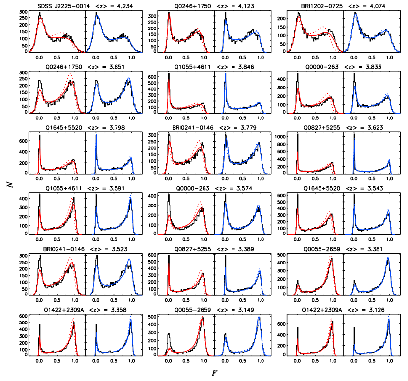
Figure 2: Fits to the Ly$\alpha$ flux probability distribution functions for QSOs in our sample, continued from Figure 1.

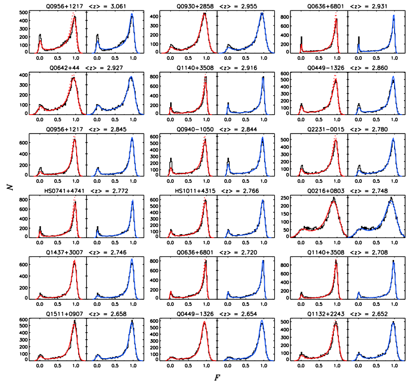
Figure 3: Fits to the Ly$\alpha$ flux probability distribution functions for QSOs in our sample, continued from Figure 1.

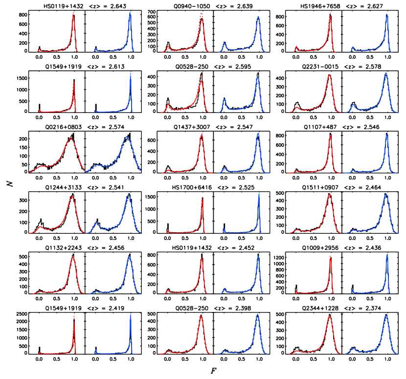
Figure 4: Fits to the Ly$\alpha$ flux probability distribution functions for QSOs in our sample, continued from Figure 1.

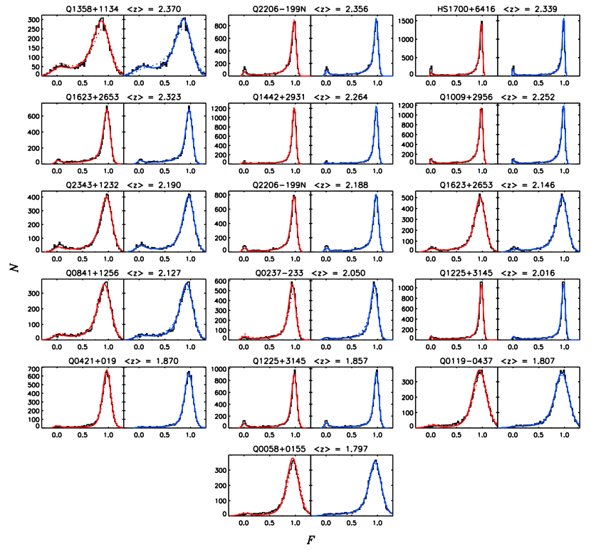
Figure 5: Fits to the Ly$\alpha$ flux probability distribution functions for QSOs in our sample, continued from Figure 1.

Figure 9: Four examples of continuum adjustments needed so that the observed flux PDFs are best fit by the theoretical distributions. Each panel shows a sample of the Ly$\alpha$ forest taken from the fitted region indicated by the QSO name and mean absorption redshift. The solid and dashed horizontal lines shows the continuum levels best fit by the MHR00 and lognormal $\tau$ distributions, respectively. The spectra have been binned to 13 km s^-1 pixels for clarity.

Figure 10: Parameters for the lognormal distribution of Ly$\alpha$ optical depths that produce the best fits to the observed flux PDFs. Here, $\mu=\langle\ln{\tau}\rangle$ and $\sigma=$ std dev $(\ln{\tau})$. The dashed lines show the best linear fits from equations (10) and (11).

Figure 11: Redshift evolution of the theoretical Ly$\alpha$ optical depth and transmitted flux distributions. The top panels show the $\tau$ distributions for the indicated redshifts and ionization rates. Bottom panels show the corresponding transmitted flux PDFs. Distributions for the MHR00 model are shown in red. Distributions for the lognormal $\tau$ model are shown in blue. Parameters for the lognormal $\tau$ distribution were calculated from fits to $\mu$ and $\sigma$ as a function of redshift (cf. equations 10 and 11). Vertical dotted lines indicate optical depths corresponding to 98% and 2% transmitted flux. The clearest differences in the predicted shapes of the flux PDFs occur at $3<z<5$. The lognormal $\tau$ distribution, which produces better fits to the data, narrows with redshift more rapidly than the MHR00 $\tau$ distribution. Hence, fewer pixels with measurable transmitted flux at $z=6$ are predicted in the lognormal case.

References

- Abel et al. (1997) Abel, T., Anninos, P., Zhang, Y., & Norman, M. L. 1997, New Astronomy, 2, 181
- Becker et al. (2006) Becker, G. D., Sargent, W. L. W., Rauch, M., & Simcoe, R. A. 2006, ApJ, 640, 69
- Becker et al. (2001) Becker, R. H., et al. 2001, AJ, 122, 2850
- Bi et al. (1992) Bi, H. G., Boerner, G., & Chu, Y. 1992, A&A, 266, 1
- Bi et al. (1995) Bi, H., Ge, J., & Fang, L.-Z. 1995, ApJ, 452, 90
- Bi & Davidsen (1997) Bi, H., & Davidsen, A. F. 1997, ApJ, 479, 523
- Bolton et al. (2004) Bolton, J., Meiksin, A., & White, M. 2004, MNRAS, 348, L43
- Choudhury et al. (2001) Choudhury, T. R., Srianand, R., & Padmanabhan, T. 2001, ApJ, 559, 29
- Coles & Jones (1991) Coles, P., & Jones, B. 1991, MNRAS, 248, 1
- Desjacques & Nusser (2005) Desjacques, V., & Nusser, A. 2005, MNRAS, 361, 1257
- Fan et al. (2002) Fan, X., Narayanan, V. K., Strauss, M. A., White, R. L., Becker, R. H., Pentericci, L., & Rix, H.-W. 2002, AJ, 123, 1247
- Fan et al. (2006) Fan, X., et al. 2006, AJ, 132, 117
- Furlanetto et al. (2004) Furlanetto, S. R., Hernquist, L., & Zaldarriaga, M. 2004, MNRAS, 354, 695
- Furlanetto et al. (2006) Furlanetto, S. R., Zaldarriaga, M., & Hernquist, L. 2006, MNRAS, 365, 1012
- Gaztañaga & Croft (1999) Gaztañaga, E., & Croft, R. A. C. 1999, MNRAS, 309, 885
- Gunn & Peterson (1965) Gunn, J. E., & Peterson, B. A. 1965, ApJ, 142, 1633
- Haiman & Cen (2005) Haiman, Z., & Cen, R. 2005, ApJ, 623, 627
- Hu & Cowie (2006) Hu, E. M., & Cowie, L. L. 2006, Nature, 440, 1145
- Hu et al. (2004) Hu, E. M., Cowie, L. L., Capak, P., McMahon, R. G., Hayashino, T., & Komiyama, Y. 2004, AJ, 127, 563
- Hui & Gnedin (1997) Hui, L., & Gnedin, N. Y. 1997, MNRAS, 292, 27
- Hui & Haiman (2003) Hui, L., & Haiman, Z. 2003, ApJ, 596, 9
- Kelson (2003) Kelson, D. D. 2003, PASP, 115, 688
- Kirkman et al. (2005) Kirkman, D., et al. 2005, MNRAS, 360, 1373
- Lidz et al. (2006a) Lidz, A., Oh, S. P., & Furlanetto, S. R. 2006a, ApJ, 639, L47
- Lidz et al. (2006b) Lidz, A., Heitmann, K., Hui, L., Habib, S., Rauch, M., & Sargent, W. L. W. 2006b, ApJ, 638, 27
- Liu et al. (2006) Liu, J., Bi, H., Feng L.-L., & Fang, L.-Z. 2006, ApJL, accepted (astro-ph/0605614)
- Malhotra & Rhoads (2006) Malhotra, S., & Rhoads, J. E. 2006, ApJL, submitted (astro-ph/0511196)
- Malhotra & Rhoads (2004) Malhotra, S., & Rhoads, J. E. 2004, ApJL, 617, L5
- McDonald & Miralda-Escudé (2001) McDonald, P., & Miralda-Escudé, J. 2001, ApJ, 549, L11
- McDonald et al. (2000) McDonald, P., Miralda-Escudé, J., Rauch, M., Sargent, W. L. W., Barlow, T. A., Cen, R., & Ostriker, J. P. 2000, ApJ, 543, 1
- Mesinger et al. (2004) Mesinger, A., Haiman, Z., & Cen, R. 2004, ApJ, 613, 23
- Mesinger & Haiman (2004) Mesinger, A., & Haiman, Z. 2004, ApJ, 611, L69
- Miralda-Escudé et al. (2000) Miralda-Escudé, J., Haehnelt, M., & Rees, M. J. 2000, ApJ, 530, 1
- Miralda-Escudé et al. (1996) Miralda-Escudé, J., Cen, R., Ostriker, J. P., & Rauch, M. 1996, ApJ, 471, 582
- Oh & Furlanetto (2005) Oh, S. P., & Furlanetto, S. R. 2005, ApJ, 620, L9
- Press et al. (1992) Press, W. H., Teukolsky, S. A., Vetterling, W. T., & Flannery, B. P. 1992, Numerical Recipers in C (2nd Ed.; Cambridge: Cambridge Univ. Press)
- Rauch et al. (1997) Rauch, M., et al. 1997, ApJ, 489, 7
- Rauch (1998) Rauch, M. 1998, ARA&A, 36, 267
- Santos (2004) Santos, M. R. 2004, MNRAS, 349, 1137
- Songaila & Cowie (2002) Songaila, A., & Cowie, L. L. 2002, AJ, 123, 2183
- Songaila (2004) Songaila, A. 2004, AJ, 127, 2598
- Stern et al. (2005) Stern, D., Yost, S. A., Eckart, M. E., Harrison, F. A., Helfand, D. J., Djorgovski, S. G., Malhotra, S., & Rhoads, J. E. 2005, ApJ, 619, 12
- Suzuki (2006) Suzuki, N. 2006, ApJS, 163, 110
- Telfer et al. (2002) Telfer, R. C., Zheng, W., Kriss, G. A., & Davidsen, A. F. 2002, ApJ, 565, 773
- Theuns et al. (2002) Theuns, T., Schaye, J., Zaroubi, S., Kim, T.-S., Tzanavaris, P., & Carswell, B. 2002, ApJ, 567, L103
- Vogt et al. (1994) Vogt, S. S., et al. 1994, Proc. SPIE, 2198, 362
- Weinberg et al. (1997) Weinberg, D. H., Miralda-Escudé, J., Hernquist, L., & Katz, N. 1997, ApJ, 490, 564
- White et al. (2003) White, R. L., Becker, R. H., Fan, X., & Strauss, M. A. 2003, AJ, 126, 1
- White et al. (2005) White, R. L., Becker, R. H., Fan, X., & Strauss, M. A. 2005, AJ, 129, 2102
- Wyithe & Loeb (2004) Wyithe, J. S. B., & Loeb, A. 2004, Nature, 427, 815
- Wyithe & Loeb (2005) Wyithe, J. S. B., & Loeb, A. 2005, ApJ, 625, 1