The 2dF-SDSS LRG and QSO (2SLAQ) Luminous Red Galaxy Survey

Abstract

We present a spectroscopic survey of almost 15,000 candidate intermediate-redshift Luminous Red Galaxies (LRGs) brighter than $i=19.8$, observed with 2dF on the Anglo-Australian Telescope. The targets were selected photometrically from the Sloan Digital Sky Survey (SDSS) and lie along two narrow equatorial strips covering 180 $\rm{deg}^{2}$. Reliable redshifts were obtained for 92% of the targets and the selection is very efficient: over 90% have $0.45<z<0.8$. More than 80% of the $\sim 11,000$ red galaxies have pure absorption-line spectra consistent with a passively-evolving old stellar population. The redshift, photometric and spatial distributions of the LRGs are described. The 2SLAQ data will be released publicly from mid-2006, providing a powerful resource for observational cosmology and the study of galaxy evolution.

1 Introduction

The Two-degree Field Galaxy Redshift Survey (2dFGRS: Colless, Dalton, Maddox et al. 2001) and the MAIN galaxy sample (Strauss et al., 2002) of the Sloan Digital Sky Survey (SDSS: York et al. 2000), have provided detailed maps of the local structure from hundreds of thousands of galaxies of all types at a mean redshift of $z\sim 0.1$, while the SDSS is also generating a large sample of more distant Luminous Red Galaxies (LRGs) with $0.25<z<0.5$ (Eisenstein et al., 2001). The present paper describes a new survey which combines the precision of the SDSS photometric survey with the spectroscopic capabilities of the Two-degree Field instrument (2dF) on the 3.9m Anglo-Australian Telescope (AAT), to extend the LRG survey from $z\approx 0.45$ to $z\approx 0.7$. LRGs constitute ideal tracers of large-scale structure at intermediate redshifts ($0.3<z<1$) because they are intrinsically luminous and spectroscopically homogeneous, and can be reliably identified photometrically. LRGs are strongly clustered, with a bias towards high density regions in ways that are believed to be well understood.

The shift in the focus of observational cosmology from determining cosmological parameters to attempting to constrain galaxy evolution and formation has accelerated over the past decade, especially since the release of the first WMAP results (Spergel et al., 2003). The spectroscopic information extracted from the 2dFGRS and SDSS has provided important clues as to the nature of galaxies in the local Universe and their recent history (Kauffmann et al., 2003; Heavens et al., 2004). Although galaxies are generally believed to form hierarchically through a succession of mergers, it appears that the many of the most massive elliptical galaxies are very old as judged from their stellar content. Thus it seems that the rate of the merger process depends strongly on the local density. A large survey of LRGs at $z\sim 0.55$ therefore has two objectives: revealing the large scale structure and clustering of matter when the universe was about two thirds of its present age, and understanding the evolution of the most massive galaxies themselves.

The SDSS LRG Survey (Eisenstein et al., 2001) is limited to $r<19.5$ by the fixed exposure time of 45m, set for SDSS spectroscopic observations in the lower redshift MAIN galaxy survey. This is well above the limit to which LRGs can be selected reliably from the SDSS imaging data. The original 2dFGRS included all galaxies with blue magnitude $b_{\rm J}<19.5$, which reached $z=0.3$ and required exposures of less than an hour on the AAT. By increasing the exposure time to 4h and targetting only the relatively rare LRGs for spectroscopy in the red spectral region, 2dF can reach $i=19.8$ and $z\sim 0.7$.

The surface density of LRG targets requires only 200 of the 400 2dF fibres within each $2\degr$ diameter field, so all the LRGs were observed in one of the two 2dF spectrographs. The other was used for a lower resolution survey of faint QSOs (Croom et al., 2006; Richards et al., 2005) which extends the earlier 2dF QSO Redshift survey (2QZ: Croom et al. 2004). The two new surveys together comprise the 2dF-SDSS LRG And QSO survey, 2SLAQ. A bonus of 2SLAQ is that there is some overlap in redshift range for the LRGs and QSOs, which will enable a direct comparison between their spatial distributions. There is also scope for investigating environmental and gravitational lensing effects, through the comparison of foreground LRGs and the absorption spectra of nearby background QSOs (cf. Bolton et al. 2004).

The 2SLAQ targets were selected within two narrow equatorial strips, each $2\degr$ wide and about $100\degr$ long running through the northern and southern Galactic caps, chosen for having good photometry at the time of the first SDSS data release (DR1: Abazajian et al. 2003). The aim of the LRG survey was to obtain spectra for 10,000 galaxies in the redshift range $0.45<z<0.7$.

This paper describes the photometric target selection, spectroscopic observations and data analysis for the LRGs, and summarises the properties of the sample. Basic cosmological parameters are being derived from the full sample, such as luminosity functions (Wake et al., 2006) and spatial correlation functions and clustering (Ross et al., 2006). Roseboom et al. (2006) investigate the incidence of star formation as a function of redshift and have identified rare ‘k+a’ galaxies which had a substantial burst of star formation within the last billion years, while Sadler et al. (2006) identify and determine the cosmic evolution of almost 400 2SLAQ LRGs which are catalogued radio sources. The 2SLAQ LRG redshifts have been used by Padmanabhan et al. (2005) and by Collister et al. (2006) and Blake et al. (2006) to validate the determination of SDSS photometric redshifts.

2 Input catalogue and LRG sample definitions

Distant LRGs were selected on the basis of SDSS photometric data (see Fukugita et al. 1996 for the definition of the $ugriz$ $AB_{\nu}$ system), using a two-colour plot of ($r-i$) against ($g-r$) and the $i$–band magnitude. Effectively, the selection uses a crude determination of photometric redshift as the 4000Å break moves through the $gri$ bands. The colour criteria are similar to those used for the Cut II sample of SDSS LRGs (Eisenstein et al., 2001), although the selection here is easier since beyond $z>0.4$ there is less confusion with lower-redshift galaxies. Targets were also required to have non-stellar images.

The selection of targets into several priority classes was done originally using the best SDSS photometry available in 2003. The later DR4 photometry (Adelman-McCarthy et al., 2006) has been used in the final redshift lists and for the diagrams in this paper. For most objects the changes amount to at most a few hundredths of a magnitude, with r.m.s. scatters of $\sim 0.01$ mag and negligible mean shifts of only $\sim 0.001$ mag in each colour. The photometry for some galaxies changed by larger amounts, due mainly to changes in how composite images were de-blended: as a result, a few tens of galaxies ($<~{}1$%) now appear to have colours inconsistent with their original selection classification.

2.1 Detailed selection criteria

After some experimentation two main samples of LRGs were defined. The primary sample (Sample 8 in the data lists) has a surface density of about 70 $\rm{deg}^{-2}$, chosen to maximise the completeness and spatial uniformity of 2dF coverage for LRGs with $z>0.45$ (see Section 3.2). The secondary Sample 9 consists of galaxies with $z\sim 0.4$, to utilise fibres which could not be assigned to primary targets. A few targets falling outside the selection boundaries were included as ‘fillers’ (Sample 0).

Fig. 1 illustrates the colour selection boundaries superimposed on the SDSS photometric data. Most galaxies of all types lie along a common locus in the lower left hand corner of this plot, becoming redder in $g-r$ with increasing redshift until the 4000Å break moves into the $r$–band at $z=0.4$. Thereafter, the $r-i$ colour becomes rapidly redder until the break moves into the $i$–band at $z=0.7$. Thus the most massive and luminous intermediate redshift galaxies, i.e. LRGs with a dominant passively-evolving population, are expected to lie along a vertical track with $g-r\sim 1.7$ in Fig. 1.

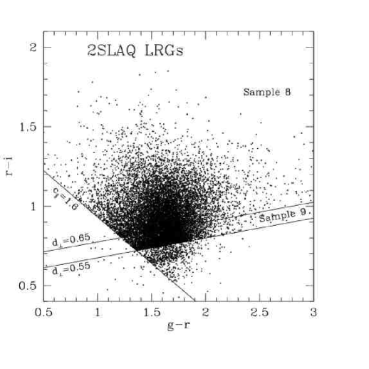
Figure 1: 2SLAQ LRG selection boundaries in the $gri$ 2-colour diagram. The primary (Sample 8) LRG targets lie in the top zone in the plot, above the diagonal lines $c_{\parallel}=1.6$ and the upper $d_{\perp}$ cut at 0.65 (see text for details). The secondary (Sample 9) objects lie between the two parallel $d_{\perp}$ cuts at 0.65 and 0.55. Most of the points below the $d_{\perp}=0.55$ cut (in the bottom right hand quadrilateral) represent lower redshift LRGs from the initial observing runs. Passively evolving LRGs with $z\sim 0.55$ are expected to lie along an approximately vertical locus in this plot, with $g-r\sim 1.7$ and with $r-i$ increasing from $\sim 0.7$ to $\sim 1.4$ as redshift increases from 0.4 to 0.7. Nearly all lower redshift galaxies of all types lie below the $c_{\parallel}$ boundary in the bottom left hand corner. The points with $(g-r)>2.3$ are mainly due to errors in the SDSS $g$-band photometry for such faint objects.

Cuts above lines of constant

$$d_{\perp}=(r-i)-(g-r)/8.0$$ (1)

(cf. Eisenstein et al. 2001) select early-type galaxies at increasingly high redshift. The top priority primary sample has $d_{\perp}\geq 0.65$ while the secondary sample has $0.65>d_{\perp}\geq 0.55$.

A second cut with

$$c_{\parallel}=0.7\times(g-r)+1.2\times(r-i-0.18)\geq 1.6$$ (2)

eliminates later-type galaxies. The colours used here are the extinction-corrected $modelMag$ colours: the definition of these and other SDSS parameters can be found in Stoughton et al. (2002) or at http://www.sdss.org/dr4/algorithms/photometry.html.

The third main selection parameter is the de-reddened magnitude in the $i$–band: the 2SLAQ LRGs have

$$17.5\leq i_{\rm deV}-A_{i}<19.8$$ (3)

where $i_{\rm deV}$ is the total magnitude based on a fit to a de Vaucouleurs profile and $A_{i}$ is the extinction in the $i$-band. This choice of a fixed limiting magnitude enables the selection of bright LRGs out to $z\sim 0.8$, although it also means that the sample at $z\sim 0.5$ includes a substantial number of fainter early-type galaxies with luminosity $\sim L^{\star}$.

Further cuts

$$0.5\leq(g-r)<3.0;\qquad(r-i)<2.0$$ (4)

eliminate objects too far from the main LRG locus, probably mostly composite objects or the result of photometric errors.

The photometric selection criteria are summarised in Table 1. The first two rows define the primary Sample 8 and secondary Sample 9, which comprise 67% and 27% respectively of the final LRG survey. 4% of the objects are in Samples 3–6, observed in March and April 2003 using somewhat different criteria (Section 2.2). The final 2% fell outside the selection boundaries and have been assigned to Sample 0.

Table 1: Photometric selection criteria.

Sample	$d_{\perp}$	$c_{\parallel}$	$i_{\rm deV}$	$g-r$	$r-i$
S8	$>0.65$	$\geq 1.6$	$<19.8$	$0.5-3.0$	$<2.0$
S9	$0.55-0.65$	$\geq 1.6$	$<19.8$	$0.5-3.0$	$<2.0$
S3	$>0.55$	$\geq 1.6$	$<19.5$	$1.0-3.0$	$<2.0$
S4	$0.45-0.55$	$\geq 1.6$	$<19.5$	$1.0-3.0$	$<2.0$
S5	$0.25-0.45$	$\geq 1.6$	$<19.5$	$1.0-3.0$	$<2.0$
S6	$>0.55$	$\geq 1.6$	$<20.0$	$1.0-3.0$	$<2.0$

Star/galaxy separation based on the SDSS images eliminates most stellar contamination from the sample. Two criteria were used,

$$i_{\rm psf}-i_{\rm model}>0.2+0.2\times(20.0-i_{\rm deV})$$ (5)

and

$$radius_{\rm deV({\it i})}>0.2$$ (6)

but some cool M-dwarf stars remain and these comprise about 5% of all targets.

Objects too diffuse to yield useful spectra using the 2 arcsec diameter 2dF fibres were eliminated by requiring $i_{\rm fiber}<21.2$ (such objects are liable to be spurious in any case). The SDSS 3 arcsec fibre diameter is used for convenience, although the 2dF fibres are only 2 arcsec in diameter.

The scatter of points on the red side of the main clump in Fig. 1, beyond $(g-r)\sim 2.3$, is mainly due to photometric errors in the SDSS $g$-band. Most points in this region have $(g-i)\sim 4.0$ and correspond to galaxies with $i\sim 19.5$ and hence $g>23$. At this very faint level the mean error in $g$ is more than 0.3 mag.

2.2 Early observations

Different cuts and priorities were used for the initial observing runs in March and April 2003. The original magnitude limit was $i_{\rm deV}<19.5$ but it became apparent that reliable redshifts could be determined to somewhat fainter limits. Tests showed that $i_{\rm deV}<19.8$ was a realistic limit in exposure times of 4 hours. The number counts are sufficiently steep that this relatively small change had two very significant consequences: the proportion of high redshift galaxies with $z>0.6$ doubled to $\sim 15$% and half of the primary targets are in the faint extension. Effectively the original limit became the new median redshift, at $i_{\rm deV}=19.48$.

Three colour-selected samples were defined originally: a top priority class consisting of all objects with $d_{\perp}\geq 0.55$ and two sparse-sampled classes with $0.45\leq d_{\perp}<0.55$ and $0.25\leq d_{\perp}<0.45$ (Samples 3, 4 and 5 respectively). These targets all had $i_{\rm deV}<19.5$ and $(g-r)\geq 1.0$. A special faint Sample 6 with $i_{\rm deV}<20$ was observed in one test field, d10, and was used to determine the optimum magnitude limit for the remainder of the survey. In addition to the different sample specifications, there were subsequent small revisions to the SDSS DR1 photometry. Most of the early observations could be reassigned to Samples 8 or 9 and nearly all of the fields have been re-observed to maintain the uniformity of the survey, but about 900 galaxies remain outside the primary and secondary samples.

3 Survey design

The AAT 2dF fibre system (Lewis, Cannon, Taylor et al., 2002) is ideally suited to this project. The LRG surface density is $\sim$70 per sq deg down to a magnitude limit of $i=19.8$, corresponding to an SDSS fibre magnitude of $r_{\rm fiber}\sim 22$. 2dF can provide reliable redshifts for over 90% of such targets in four hours, in average conditions. Atmospheric refraction limits the maximum time for which a given 2dF configuration can be efficiently observed to about 3h for fields on the equator, so most fields were observed on two consecutive nights.

The most practical survey design was two narrow strips along the celestial equator, one in each Galactic hemisphere, given the early SDSS photometric coverage and the requirement to work through complete nights. There was also a desire to overlap with previous surveys such as 2QZ (Croom et al., 2004) and the Millenium Galaxy Survey (Liske et al., 2003; Driver et al., 2005) and to enable follow-up observations from large telescopes in both hemispheres. The northern strip runs from 8.2h to 15.3h in RA, broken into five sub-strips to utilise the best photometric data; the southern strip runs from 20.6h to 4.0h. Each strip can be covered by a single row of overlapping 2dF fields.

The ends of the strips come close to Galactic latitude $20\degr$ and thus suffer from significant extinction of up to 0.4 mag in $g$ (based on the maps of Schlegel, Finkbeiner & Davis 1998), plus substantial foreground star contamination. Priority was therefore given to fields nearer the centre of each strip with $|b|>40\degr$ and extinction $A_{g}<0.2$ mag. Fig. 2 shows the layout of the target strips and the 2dF fields actually observed. There is considerable imbalance between the two strips, with the northern strip containing more than two thirds of the data and having much higher completeness. This was an accidental consequence of the nights scheduled and variable observing conditions.

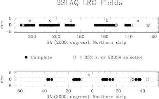
Figure 2: Layout of the 2dF 2SLAQ fields within the northern (upper) and southern (lower) Galactic strips. Filled circles denote fully observed fields, i.e. with redshift completeness $\geq 85$%. Open circles represent fields with completeness $<85$% or with non-standard selection criteria. The letters ‘a’-‘e’ and ‘s’ signify the sub-strips and are used as the first character of the field names.

3.1 Tiling pattern

The principal objective was to maximise the total number of objects in a photometrically well-defined sample, with good coverage on different spatial scales and minimal incompleteness. For simplicity it was decided to use a fixed field separation. For the initial observations in March and April 2003 the centres were set $1\degr$ apart but this was increased to $1.2\degr$ for all subsequent observations, following modelling tests of the yield.

Two strategies helped to maximise the fraction of targets which were observed. About 28% of the targets lie in the overlap regions of adjacent 2dF fields. Targets which had been observed in the configuration for one field were given lower priority in the adjacent fields. A sequence of alternate fields was observed first, followed by the partially overlapping fields in a second pass along the strip. This led to independent repeat observations for a few percent of the total sample, giving a valuable check on the internal accuracy of the data. The second strategy arose because each field was observed on two or more nights. A significant fraction of the targets, mainly the brighter galaxies and most of the M-stars, had good spectra and unambiguous redshifts after only one night. Typically some 10–20% of the fibres could then be re-allocated to new targets. This helped in crowded fields in particular, since due to physical constraints 2dF fibres have a minimum separation of at least 30 arcsec.

3.2 Target distribution across the field

Tests of the 2dF configure software showed that the algorithm which assigns fibres to targets could introduce significant patterns into the distribution of observed objects across the 2dF field. The main effect was a discontinuity in density at $0.25\degr$ radius, if the mean number of targets per field in the input catalogue was much higher than the number of fibres. There could also be systematic effects depending on the ordering of the input catalogue. Both effects were avoided in the 2SLAQ surveys by keeping the surface density of the top priority targets below 70 $\rm{deg}^{-2}$ and by randomising the order of the targets in the input catalogue.

There are instrumental constraints on the targets accessible to 2dF. The nominal $2\degr$ field can be up to $2.1\degr$ in diameter, but this varied slightly during the survey due to both hardware and software limits. There are also 20 small triangular regions around the edge of the field which are inaccessible to the fibres feeding one spectrograph. The net result is that the effective area of the survey can be approximated by a row of overlapping $2\degr$-diameter circles. Fig. 3 shows the distribution of targets across the 2dF field, for all objects in the final redshift catalogue. There is a slightly lower density of points towards the right hand edge of the field due to the asymmetrical distribution of sky fibres (see Section 4.2). Both this density gradient and the empty triangles on the eastern and western edges are largely eliminated when the data from overlapping fields are combined, but the northern and southern triangles remain.

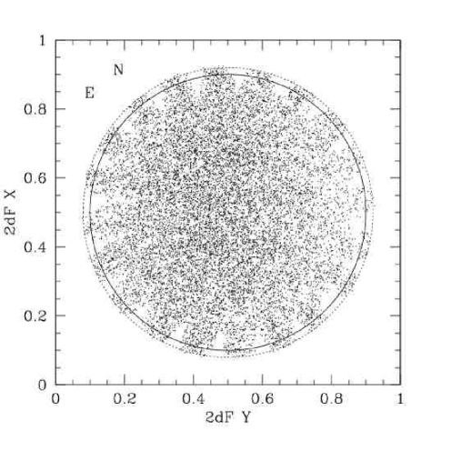
Figure 3: The distribution of LRG targets across the 2dF field, with north to the top and east to the left. The dotted circle represents the nominal $2.1\degr$ field diameter; the solid circle at $1\degr$ radius indicates the effective area covered. The empty triangles around the edge are inaccessible to the fibres feeding the single spectrograph used for the LRGs. The lower density towards the right-hand side of the field is due to the allocation of 20–30 of the western fibres to sky: those fibres feed the central rows in the spectrograph camera.

3.3 Biases in the targets observed

In addition to the inaccessible regions shown in Fig. 3, each fibre button has a large ‘footprint’ with a long tail due to the fibre, which runs across the front of the 2dF field plate. It is never possible to access targets within 30 arcsec of another which has already had a fibre allocated, and in some directions the exclusion zone is much larger. There is therefore a strong intrinsic bias against observing close pairs of galaxies, and very few fibres can be allocated to members of one cluster. This bias is partially overcome within the overlap regions of adjacent 2dF fields, and a few fields were independently observed in different runs. The bias is also alleviated by the policy of re-allocating some fibres after the first night on a given field (Section 3.1). However, there must remain a substantial bias against close pairs of targets and the level of incompleteness will have to be assessed by comparing the objects actually observed with the full input catalogue.

There is a similar conflict between the LRGs and QSOs, since the two classes of objects were observed simultaneously. Thus, although one of the strengths of 2SLAQ is having samples of LRGs and QSOs in the same fields and within the same redshift range, there is a bias against QSOs which lie near LRGs since the LRGs were given higher priority than the QSOs in the allocation process.

4 Observations

4.1 Spectrograph set-up

The LRGs were observed with 2dF Spectrograph Number 2, using a 600 lines mm^-1 $V$ grating. The detector was a Tek1024 CCD with $1024\times 1024$ pixels, giving a dispersion of 2.2Å pixel^-1 and an effective resolution of about 5Å or $R\sim 1000$. Almost all the spectra were taken with the central wavelength set to 6150Å, covering the range 5050Å to 7250Å. This enables secure determination of redshifts for $z>0.3$ using the Ca II H&K lines and the detection of [O II] 3727Å down to $z=0.35$. For the first observing run in March 2003 the central wavelength was set to 6350Å but almost no useful data were obtained beyond 7250Å, due to telluric features which did not cancel well in the low dispersion 2dF spectra. More details of the spectrographs and their performance are given in Lewis, Cannon, Taylor et al. (2002).

4.2 Sky fibres

A subset of the 2dF fibres was assigned to clear sky positions, after checking the SDSS images. These are used to determine a median sky spectrum which is subtracted from all target spectra. For each frame 30 fibres were assigned to sky (later reduced to 20, after tests showed that this resulted in negligible degradation). These sky fibres were selected to lie in the central half of the CCD (i.e. between spectra 50 and 150) to keep the sky spectra uniform, although this results in some mismatch to spectra at the edges of the CCD due to optical distortions in the camera. In principle it is possible to correct for these but this has not yet been implemented in the 2dF software. The fibres which feed the centre of the CCD happen to lie on the western side of the 2dF field, which causes the slight density gradient seen in Fig. 3.

4.3 Observing pattern

The standard pattern was to take sets of seven exposures per field: a quartz lamp flat-field, an arc lamp exposure using 4 Cu–Ar lamps and 2 He–Ar lamps, $4\times 1800$s exposures on the targets and a final arc exposure. Thus in good conditions four or occasionally five sets of observations were obtained per night and four 2dF fields could be fully observed in two nights. In poor conditions the observations were extended over extra nights, until the required mean signal-to-noise per pixel (S/N) (and hence redshift completeness fraction) was reached.

The 2SLAQ surveys were supported approximately equally by the Australian and British time assignment panels, plus a few Director’s discretionary nights, to give a total allocation of 87 nights between March 2003 and August 2005. On average about 60% of the time was useable. A total of 102 datasets was obtained for 80 2dF fields, 54 in the northern strip and 26 in the south. Observations were deemed to be complete (i.e. reliable redshifts for at least 85% of the primary targets) for 72 fields while 8 are either incomplete or used non-standard selection criteria. The final yield was very close to one completed field per allocated night, about half of the best possible rate. This is lower than the overall fraction of clear time because 2dF cannot be re-configured quickly.

The 80 distinct fields which were observed are illustrated in Fig. 2 and all the datasets are listed in Appendix A, along with various quality parameters which are discussed in Section 5.5. Some fields have more than one dataset because data were obtained in separate observing runs, sometimes with different parameters or target selections, and were reduced independently. There is some scope for combining such datasets before analysis which would lead to better quality spectra for repeated targets, but the gain in redshift completeness will be very small.

Given that it was impossible to cover entire strips in the time available, the aim was to observe several continuous sub-strips within each Galactic hemisphere. In the event, the time allocated and the observing conditions led to more than twice as much data being obtained in the northern strip as in the south. Nine separate sub-strips have been observed with varying levels of completeness. The proportion of primary (Sample 8) input targets for which reliable redshifts were obtained reaches 90% in the best regions such as northern sub-strips ‘b’ and ‘d’, each of which is $\sim 17\degr$ long. Each of these sub-strips covers a volume of space comparable to that observed in the northern 2dFGRS strip, since the angular extent of the latter was about five times larger but the mean redshift was only a fifth as high.

5 Data reduction and analysis

5.1 Extracting the spectra

All of the raw data have been analysed using the AAO 2dfdr software (Bailey, Heald & Croom, 2004). For each field, the location of the fibres on the CCD was determined using a quartz lamp exposure which was also used as a flat field to remove pixel-to-pixel sensitivity variations. Two arc exposures provided wavelength calibration. All spectra were scaled according to the relative throughput of the fibres, as determined from the strongest night sky lines, and a median sky spectrum was subtracted from each object spectrum. The different frames for each field were combined using mean flux weighting, which takes account of the variable signal levels arising from changes in ‘seeing’, transparency or exposure time; cosmic ray events were removed during this final step.

The 2dfdr software was developed for the analysis of the 2dFGRS/2QZ data. For those surveys, the data for each field consisted of several similar frames with precisely the same 200 targets, all taken on the same night. The 2dfdr software was modified during the course of the 2SLAQ surveys to cope with data taken on different nights, sometimes with significant changes to the central wavelength and often with altered allocations of fibres to targets.

5.2 Redshift determination

The LRG redshifts were derived using a modified version of the Zcode Fortran program, developed by Sutherland (1999) and others for the 2dFGRS spectra of low redshift galaxies (Colless, Dalton, Maddox et al., 2001). That program determined two independent redshifts whenever possible, one based on discrete emission lines and the other using cross-correlation with a set of template spectra. The higher resolution 2SLAQ LRG spectra cover only half the wavelength range and the targets have been photometrically selected to be predominantly passively evolving early-type galaxies at much higher redshifts ($0.3<z<0.8$). Thus it is rarely possible to derive a secure redshift using emission lines alone: the only line which is common is [O II] at 3727Å, detected by the Zcode in about 20% of the spectra. The 2SLAQ version of the Zcode derives redshifts by cross-correlating each spectrum against a set of templates and uses any emission lines only as a check on the cross-correlation results.

The cross-correlations are done using the method of Tonry & Davis (1979), which involves Fourier transformation of all the spectra and templates. The program selects the most plausible redshift for each object and assigns a quality parameter ‘Q’, which is a measure of the consistency and reliability of the initial set of redshift estimates. Another indicator of the reliability of the redshift is given by the Tonry & Davis (1979) parameter ‘$r$’ (called $r_{\rm x}$ here to avoid confusion with the photometric $r$), which measures the height of the cross-correlation peak relative to the general noise level. The spectrum, cross-correlation function and redshift for each target are shown on an interactive graphic display. The operator can either accept the automatic redshift or choose a different value (e.g. by making alternative identifications of strong features or by selecting a different template). The operator assigns an independent quality parameter to the reliability of each redshift.

The LRG version of the Zcode can be run in several modes: the basic fully interactive mode in which every spectrum is visually checked; a quick mode in which only spectra with low quality redshifts are inspected; and a fully automatic mode. The advantage of inspecting every spectrum is that unusual or extreme objects can be identified, including composite spectra; the automatic mode has the advantages of being more consistent and objective. The semi-automatic ‘quick’ mode provides a good compromise between the two methods and is normally used for initial data reductions at the telescope.

Given the rather homogeneous 2SLAQ spectra, it has proved possible to tune the automatic Zcode to give very reliable results for most objects. Fewer than 1% of the galaxies give significantly discrepant redshifts from two independent analyses of the same dataset or from repeat observations of the same targets (Section 6.1). A majority (72%) of the redshifts for the initial data release have been derived automatically, without visual inspection. Some datasets from each observing run have been re-analysed in fully interactive mode to verify that the error rate remains low.

All redshifts have been corrected to be heliocentric. Information on the templates and other details specific to the redshifting of the 2SLAQ LRGs are given in Appendix B.

5.3 The redshift quality parameter $Q$

The principal indicator of LRG redshift reliability is the parameter $Q$. Note that $Q$ does not necessarily indicate the quality of the actual spectrum. Although the two are strongly correlated in general, there are cases where a very poor spectrum yields an unambiguous redshift, and conversely. Two quality values are output by the Zcode: the automatic value ($qa$) set by the code itself, and the operator value ($qop$) set during the visual inspection of the data. The preferred value is generally the operator value, where both exist.

The definitions of the operator values are as follows:

$Q=4$: A good spectrum with an unambiguous redshift (usually $r_{\rm x}>10$), based on several strong features.

$Q=3$: A single strong cross-correlation peak (with $r_{\rm x}>5$) and some obvious features (most often H&K, G-band and/or Balmer lines).

$Q=2$: A plausible redshift but not completely convincing ($r_{\rm x}>3.5$), or where alternative redshifts are possible.

$Q=1$: A spectrum where no believable redshift can be found.

In each case, the presence of [O II] 3727Å emission (or, rarely, [O III] at 5007Å) at the absorption redshift can be used to increase the $Q$ value by 1 unit (but with $Q=4$ remaining the maximum for $qop$). Checks on multiply-observed objects from overlapping fields, and from repeat observations of the same sets of targets, show that the reliability of the different classes is $>99$% for $Q=4$, $\approx 95$% for $Q=3$ and $\sim 50$% for $Q=2$ (see also Section 6.1).

The automatic quality parameter $qa$ is derived somewhat differently but produces very consistent results. The evaluation is done in two stages: first the cross-correlation results are compared for the full set of templates to determine the parameter $qx$ for the most probable redshift (i.e. the one which gives the highest $r_{\rm x}$ value), and then the list of possible emission lines is checked for any identifications at the same redshift. The $qa$ value is also based on the consistency of the redshift across the set of templates. The M-stars are dealt with slightly differently, since they only ever fit one template (and that template, T8, never gives a correct redshift to any galaxy). $qa$ takes values in the range 0 to 5.

Comparisons between automatic and manual (i.e. fully interactive) analyses of the same datasets show good agreement between the two sets of $Q$ values. In particular, it is very rare to get any discrepancies between redshifts for which both methods give $Q\geq 3$, which comprise 90% of the targets for most datasets. A few percent of targets lie on the $Q=2-3$ borderline and these sometimes show discrepant redshifts, as is to be expected.

5.4 Quality of datasets

The overall quality of each dataset (i.e. each set of combined frames for a given 2dF field) can be evaluated in several ways, using four global parameters listed in Table 3 in Appendix A. These parameters are the number of raw data frames, $N_{\mathrm{exp}}$; the mean S/N per pixel; the mean difference between the logarithm of the counts obtained and the expected magnitudes of the targets, $D_{\mathrm{mag}}$, using here the SDSS $r_{fiber}$ parameter; and the percentage of targets with reliable redshifts. The redshift success rate, defined as the fraction of targets which have redshift reliability $Q$ of 3 or more, is the most important one for the LRG survey, while the mean S/N should be the most reliable measure of overall quality. The observing strategy attempts to minimise the variations in mean S/N by taking more frames in poor conditions, but this is only partially successful since non-statistical errors begin to become significant when many frames are combined.

Fig. 4 shows the correlation between $z$ success rate and mean S/N (per pixel, per object) for all the datasets listed in Table 3. The northern Galactic strip has systematically better data than the southern strip, mainly due to better weather conditions. Datasets for which $S/N>5$ always have $z$ completeness $>90$% while $S/N>4$ normally results in completeness of more than 85%, the level chosen as the practical limit for deciding when to terminate the observations of a field. Most of the datasets with low completeness were re-observed to give higher final redshift completeness. Data from fields with less than 85% final completeness are retained in the LRG catalogue but must be treated with caution in any statistical studies. Nearly all the datasets with S/N$>6$ are for northern fields observed early in 2003, when a brighter magnitude cut-off was used.

Figure 4: The redshift success rate for each dataset as a function of mean S/N per pixel per object. The redshift completeness can fall catastrophically when the mean S/N is below 4.0 (vertical dotted line): the observations were repeated for most such datasets. The horizontal dotted line marks the 85% success rate used as the threshhold for deciding that the observations of a field were complete.

5.5 Completeness and uniformity of the survey

The 2SLAQ LRG survey is spatially incomplete (see Fig. 2) and has a variable redshift success rate (Table 3). However, a particular effort has been made to maximise the completeness for the primary targets within several continous sub-strips. The top panel of Fig. 5 shows the number of potential targets in each field of the northern strip for Samples 8 and 9, with considerable cosmic variance between fields. The middle panel shows the percentage of primary targets with reliable redshifts, which is close to 90% on average and reasonably uniform. This is the overall completeness, i.e. the fraction of targets observed multiplied by the redshift success rate. The bottom panel of Fig. 5 gives the equivalent plot for the secondary Sample 9 objects, for which the completeness is much lower and much less uniform, ranging from 20% up to 90%. Sample 9 utilised only those 2dF fibres which could not be placed on primary targets: it tends to be least complete in the highest density fields.

The completeness is particularly poor for the low Galactic latitude fields a01 and a02, which were observed only with the original 2003 selection criteria. Similarly, the southern field s01 was abandoned after its high levels of stellar contamination and foreground reddening were recognised.

Figure 5: The completeness of data for targets in the northern strip. The top panel shows the number of potential targets in each 2dF field, for the primary Sample 8 targets (solid histogram) and the secondary Sample 9 targets (dotted histogram). The middle panel shows the percentage of primary targets for which reliable redshifts were obtained (the horizontal dotted line marks 90% overall completeness) while the bottom panel shows the same for the secondary sample. The labels in the top panel give the names of the 2dF fields within each sub-strip.

It is difficult to define the precise boundaries of the 2SLAQ survey, given the overlapping tiling pattern, the inaccessible triangles near the edge of the field (Fig. 3) and the fibre re-allocation observing strategy. One simple way to derive a very complete sample is to work in rectangles which lie completely within the patterns of overlapping 2dF circles. Two such inscribed rectangles can be drawn in the well-observed northern sub-strips ‘b’ and ‘d’, containing over 30% of the entire LRG survey. The targetting completeness is 94.5% for the primary Sample 8 and the redshift completeness is 96.7%, giving an overall completeness of 91.4%.

The best way to evaluate the completeness of the 2SLAQ survey, and to calculate its effective total area, is to create a spatial mask including all objects in the input lists which could in principle have been accessed by 2dF from at least one of the observed field centres. This has been done by Wake et al. (2006) and the resulting mask will be made available as part of the survey data.

5.6 Output lists

Two ascii listings are generated by the Zcode for each 2dF field. One, filenamez.rz, gives the target names, positions, fibre numbers, redshift parameters and some photometric and quality data, with one line for each spectrum analysed. The second, filenamez.zlog, gives much more data on the redshifting process, including the results of cross-correlating every target against each template and lists of strong emission lines found. Some overall statistics, such as the numbers of reliable redshifts and the mean S/N of all the spectra, are also recorded. The *z.rz files are concatenated and sorted to generate the final output redshift lists for the LRG survey.

The target names follow the standard IAU convention, i.e. using the truncated J2000 position in Right Ascension and declination. These are quoted to a precision of 0.1 arcsec, which ensures unambiguous identification of the objects. However, one drawback is that sometimes the names can change slightly when the input SDSS photometric data are revised, or when positions are converted between arcsec (and seconds of time) and decimal degrees or radians. The only safe way to make cross-identifications with other catalogues is to look for positional coincidences, rather than identical names.

Multiple observations were made for about 20% of the targets, either because they lay in the overlap regions of adjacent 2dF fields or because entire fields were re-observed. The 2dfdr and Zcode software originally assumed that all observations for a given dataset were taken using the same configuration of 200 fibres with the same spectrograph set-up. Thus two or more independent spectra were obtained for many objects and two catalogues have been generated, one listing every spectrum obtained and the other with a single entry for each discrete object observed. The latter, which is the basic redshift catalogue, simply uses the best available redshift for each object. The selection is based on the redshift quality parameter $Q$, or on mean S/N when two spectra give the same $Q$.

Better spectra could be obtained for some repeated objects by combining the independent spectra from different observing runs. Every spectrum should also be checked visually, to pick up any very peculiar objects or ones where the automatic redshifting has missed some obvious feature such as a composite spectrum. However, this will make very little difference to the actual redshifts: there should simply be a small increase in the number which are reliable. The radio sources which comprise about 3.5% of the 2SLAQ LRGs (Sadler et al., 2006) have been used as a quality control sample and confirm this expectation.

The redshift lists are held in the 2SLAQ team archive at the University of Queensland, http://lrg.physics.uq.edu.au/ and can be accessed via links at the University of Portsmouth (http://www.2slaq.info), at the AAO (http://www.aao.gov.au) and elsewhere. The archives also contain the full sets of 2dF reduced data, the individual LRG spectra and sets of SDSS postage stamp images. A catalogue of the best available redshift for every object observed is being released in mid-2006, together with the basic SDSS photometric data and other parameters. The final full set of 2dF spectra and SDSS photometry will be made publicly available once the data re-reductions are complete.

5.7 Examples of the spectra

A number of representative galaxy spectra, plus one of the contaminating M stars, are illustrated in Fig. 6.

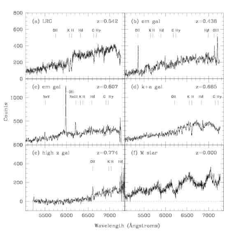
Figure 6: Examples of 2SLAQ LRG spectra, with some major features identified. No flux calibration has been applied. The residuals from a few strong night sky lines have been excised, while the dips near 6850Å and 7200Å seen in several spectra are due to uncorrected atmospheric absorption bands. Spectra (b) to (e) have been lightly smoothed. The redshifts are indicated in the top right hand corner of each panel: (a) J110954.40+004843.1, a relatively high S/N spectrum of a typical LRG with redshift $\sim 0.55$; (b) J022459.77$-$000156.4, a low redshift 2SLAQ galaxy with both [O II] and [O III] in emission; (c) J225439.77$-$001501.2, a rare emission line galaxy with higher excitation [Ne III] and [Ne V] as well as [O II]; (d) J212907.12+002405.4, one of the rare ‘k+a’ LRGs with prominent Balmer lines in absorption and a weak 4000Å break; (e) J122554.82$-$000752.4, one of the highest redshift 2SLAQ LRGs with $z=0.774$; (f) J124853.73$-$010332.7, a typical foreground M-star.

Fig. 6(a) is a good spectrum of J110954.40+004843.1 at $z=0.542$, a typical 2SLAQ LRG close to the median redshift. The H&K lines of Ca II and strong 4000Å break are unambiguous determinants of the redshift and several other stellar absorption features are very obvious, but no emission lines are detectable.

(b) is the galaxy J022459.77-000156.4 at $z=0.438$, with both [O II] and the [O III] doublet in emission. This galaxy is close to the lower redshift cut-off for 2SLAQ LRGs and shows why the spectra very rarely yield reliable emission-line redshifts, since both [O II] and [O III] fall within the 2SLAQ spectral window for only a very narrow redshift range.

(c) is J225439.77-001501.2 at $z=0.607$. The best cross-correlation used the K-type stellar template but the redshift reliability was low. The redshift is secure only because high excitation emission lines of [Ne V] 3426Å and [Ne III] 3870Å are clearly present.

(d) is J212907.12+002405.4 at $z=0.665$, one of the relatively rare ‘E+A’ or ‘k+a’ galaxies in the 2SLAQ sample (Roseboom et al. (2006)). These galaxies show very strong Balmer absorption lines, with H-$\epsilon$ making the Ca II H line apparently much stronger than K, and a relatively weak G-band and 4000Å break. [O II] 3727Å emission is often present. These galaxies are understood to have had a substantial episode of star formation up to $5\times 10^{8}$ years ago.

(e) is J122554.82-000752.4 at $z=0.774$, one of the highest redshift galaxies in the sample. The continuum is close to zero over much of the spectrum, but the strong H&K lines plus [O II] yield an unambiguous redshift. Like many high redshift LRGs, this galaxy shows ‘k+a’ features similar to Fig. 6(d). This spectrum was obtained in March 2003 with the wavelength range shifted 200Å redwards compared with all later spectra: it is apparent that the data beyond 7250Å were not useful.

(f) is J124853.73-010332.7 at $z=0.0$, a typical M-star with very characteristic molecular absorption bands. About 5% of the targets are foreground Galactic M-dwarfs; contamination by other stellar types is negligible.

6 Reliability and accuracy of the redshifts

Considerable effort has gone into making the catalogue of 2SLAQ LRG redshifts complete and reliable. This involves not only determining good redshifts for as many LRGs as possible but also identifying those objects that are not LRGs within the redshift range of primary interest. Usually $\sim 90$% of the targets give unambiguous redshifts in a first pass through the data. By far the most common cause of failure is low S/N, due to either target faintness or fibre misplacement. A few targets ($\sim 0.1$%) fail to give a reliable redshift due to other causes such as instrumental artefacts or proximity to bright stars, but these are not liable to introduce any systematic bias into cosmological analyses of the LRGs.

About twenty composite spectra have been found and more would no doubt be revealed by systematic searches: the Zcode software finds only the most probable redshift for each target. Most of the composites consist of an M-star plus a galaxy while a few show a second emission line redshift on top of the primary spectrum. The photometric data are unlikely to be meaningful when a strong M-star signature is present so the redshift is generally given as zero in such cases. Any secondary redshift is noted since it may still be useful, e.g. if a target is identified as a radio source.

6.1 Redshift reliability

Several internal checks have been carried out by comparing different analyses of the same data set, different sets for the same field, and finally targets which have been observed independently in different fibres from different configurations.

The best datasets yield very high redshift completeness, i.e. reliable ($Q\geq 3$) redshifts for $>95$% of the targets. Comparisons between analyses of such sets by different Zcode operators show excellent agreement in the preferred redshift, with only a handful of objects differing, mostly among those with $Q=2$. There can be more spread in the $Q$ ($qop$) values since this is a somewhat subjective measure, but nearly all agree within 1 unit.

Several pairs of datasets for the same field have been compared. The number of significant redshift discrepancies, i.e. where two different redshifts both with $Q>2$ are claimed, averages less than 1%. Most of these are cases where one or both cross-correlation redshifts are on the borderline between quality 2 and 3, a few are due to the automatic code missing an obvious emission line fit, a few are due to manual operator errors, and a couple have been composite spectra with two valid redshifts.

The largest set of independent spectra, mostly taken in different configurations using different fibres, consists of repeat observations in 2005 of 1253 objects from the first two years. Just 9 pairs were significantly discrepant, in that two apparently good redshifts with $Q\geq 3$ differed by more than 0.01. Three of these were composite star+galaxy spectra where both redshifts were valid and one was a very unusual emission line galaxy. The remaining five each had one unambiguous redshift while the other was a marginal redshift close to the boundary between $Q=3$ and $Q=2$. Thus the error rate is only about 0.5%.

An external check of redshift reliability is provided by the SDSS LRG Survey which has some overlap in the redshift range $0.3<z<0.5$ (see Section 6.3). The redshifts agree to within 0.002 for 143 of 145 galaxies in common, the only discrepancies being for 2 of the 3 galaxies for which the 2SLAQ redshift were unreliable, i.e. with $Q=2$. The $Q\geq 3$ redshifts are evidently 100% reliable in this comparison set.

6.2 Significance of signal-to-noise ratio

The redshift reliability depends strongly on S/N. Histograms of S/N for the objects with and without reliable redshifts are shown in Fig. 7. The overall success rate (i.e. $Q\geq 3$) for all targets in Samples 8 and 9 was 92%. This rises to 99% for spectra with S/N $>4$ but falls to just over 50% for the $\sim 5$% of spectra with S/N$<1.5$.

Figure 7: Histograms of mean S/N per pixel for all Sample 8 and 9 spectra which gave reliable redshifts (solid line) and for those which failed (dotted line, shaded histogram). 95% of spectra with S/N $>2$ are adequate for determining redshifts.

Fig. 8 shows the run of S/N per pixel with redshift, for spectra which yielded reliable redshifts. The average S/N decreases as $z$ increases, from a median value of about 5.0 at $z=0.45$ to 3.0 at $z=0.65$. This is partly because the galaxies become systematically fainter with redshift and partly because only a small section of spectrum redwards of the 4000Å break remains within the 2SLAQ window. Night sky emission lines and atmospheric absorption features beyond 6800Å exacerbate the latter effect. The overall shape of the distribution is a reflection of the plot of redshift against magnitude (see Fig. 10, Section 8). A few galaxies are listed with negative S/N, which is clearly non-physical. These are usually spectra where the continuum drops below zero due to over-subtraction of the sky or scattered light. The redshift code can sometimes still give a reliable $z$ value in such cases.

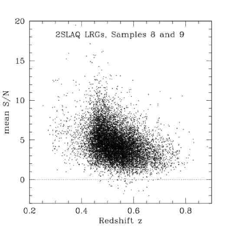
Figure 8: Mean S/N as a function of redshift $z$, for all primary (Sample 8) and secondary galaxies with reliable redshifts. A few objects fall below the S/N = 0 boundary (dotted line) due to errors in sky subtraction, but retain sufficient features for a reliable redshift determination.

6.3 Redshift accuracy

The comparison with the SDSS LRGs provides a quantitative check on the accuracy of both sets of redshifts. There is a mean shift of 0.00031 between the two sets, arising from the use of air wavelengths for the 2SLAQ templates and vacuum wavelengths by the SDSS. The rms difference for the sample is 0.00040, after removing two discrepant 2SLAQ redshifts and a further three outliers with $dz\sim 0.002$. This implies that the internal accuracy of the $Q\geq 3$ 2SLAQ redshifts is no worse than $\pm 0.0003$.

A similar check can be derived from repeated 2SLAQ spectra. The rms scatter between sets of data taken in different years was typically about 0.0006. Some of this scatter arose from differences between the templates, partly intrinsic and partly due to calibration errors. When the velocity zero-points were corrected (Appendix B1) the rms scatter fell to 0.00045. This again implies an internal error in a single redshift of $\pm 0.0003$.

7 Survey statistics and coverage

7.1 Overall redshift statistics

The overall statistics for the 2SLAQ LRG survey are summarised in Table 2. Nearly 18500 spectra were obtained over three years, for 14978 discrete objects. 13784 of these (92%) have good ($Q>=3$) redshifts. About 5% of the targets turn out to be foreground M stars, leaving a total of 13121 galaxies of which 11451 have $z>0.45$.

These statistics are for all 80 discrete 2dF fields which were observed. A few fields have low quality data or were observed with only the original photometric selection criteria. In particular, fields a01, a02, s01 and s12 have less than 50% completeness for the primary Sample 8 targets and should be ignored in statistical analyses (see Table 3).

Three columns of figures are given in Table 2. Column 1 is for the primary Sample 8 which is the most complete and homogeneous sample, column 2 for the secondary Sample 9 and column 3 for all objects observed. Sample 9 is photometrically homogeneous with high redshift completeness and only 1% contamination by M-stars, but it has very variable spatial completeness.

The first two rows of Table 2 give the number of discrete objects observed and the number which have reliable redshifts. Row 3 gives the number of contaminating stars (virtually all M-stars). Row 4 is the number of bona fide LRGs and row 5 gives their median redshift. The final three rows give the numbers of galaxies in the primary redshift target range of $0.45<z<0.7$ and in the low and high redshift tails. Most of the $z<0.45$ galaxies are either in Sample 9 or were observed in the first semester, before the selection criteria were refined. Virtually all of the highest redshift galaxies, with $z>0.7$, are from Sample 8.

Table 2: Target statistics.

Selection	Sample 8	Sample 9	All
observed	10072	3977	14978
$z$ ($Q\geq 3$)	9307	3624	13784
stars	551	37	663
LRGs	8756	3587	13121
median $z$	0.55	0.47	0.522
$0.45<z<0.7$	8289	2647	11196
$z<0.45$	214	935	1664
$z>0.7$	253	5	261

7.2 Spatial coverage of the survey

The total area covered by the 2SLAQ survey is approximately 180 $\rm{deg}^{2}$, calculated as the number of fields observed multiplied by the effective area of each field, corrected for edge effects and the overlap between adjacent fields. However, this is not a particularly useful number since the completeness of the survey varies significantly from field to field and between the different samples in each hemisphere. Further complications arise from the constraints on placing 2dF fibres in close proximity, mentioned in Section 3.3.

A more useful statistic for comparison with other surveys is the effective area of the survey, defined as the total number of targets with reliable redshifts divided by their mean density in the input catalogues. This gives an effective area of approximately 135 $\rm{deg}^{2}$ for the Sample 8 targets and 90 $\rm{deg}^{2}$ for Sample 9. A more careful calculation by Sadler et al. (2006), using the detailed survey mask of Wake et al. (2006), revises these areas to 141.7 $\rm{deg}^{2}$ and 93.5 $\rm{deg}^{2}$ for Samples 8 and 9 respectively.

These figures imply that the overall completeness of the primary sample is only about 75%, falling to 50% for the secondary sample. However, as noted in section 5.6, the completeness of the primary sample rises to $\sim 90$% in the best-observed regions.

8 Properties of the LRG sample

8.1 Redshift distributions

A histogram of the redshifts of all the 2SLAQ galaxies is shown in Fig. 9. It is obvious that the SDSS colour and magnitude selection criteria produce a very clean sample of high redshift galaxies. Almost all the targets have $0.3<z<0.8$, apart from $\sim 5$% contamination by foreground M-stars. The dotted line is for the entire set of 2SLAQ LRGs, including the early samples with somewhat different selection criteria which contribute most of the low-redshift tail. The solid line is for the primary sample which has median redshift 0.55 and 80% of the redshifts within $0.45<z<0.7$, as desired. The sharp lower cut-off is set by the colour selection while the declining tail for $z>0.6$ is due to the $i<19.8$ magnitude limit. The secondary (Sample 9) galaxies, shown by a dashed line, have median redshift 0.47.

Figure 9: Redshift histograms for the 2SLAQ LRGs. The solid line is for those objects in the primary sample (8) and the dashed line is for the secondary sample (9). The histogram for all objects with reliable redshifts is shown as a dotted line. The spike at $z=0$ represents the 5% contamination by foreground M-stars. The effectiveness of the 2SLAQ photometric selection for $z\sim 0.5$ galaxies is evident.

Fig. 10 compares the redshift distribution of the 2SLAQ LRGs with that of the SDSS LRGs (Eisenstein et al., 2001) and the 2dFGRS galaxies of all types (Colless, Dalton, Maddox et al., 2001), in each case counting only the galaxies lying within the same $2\degr$ wide northern equatorial strip. The three surveys are complementary and together give good redshift coverage from $z=0.02$ to $z=0.7$. There is significant overlap between the 2SLAQ and SDSS LRG samples at $z=0.4$ but 2SLAQ provides a much higher space density of galaxies with $z>0.4$ than any other current survey, as is needed for mapping the 3–D structure.

Figure 10: The redshift distribution of three surveys in the same $2\degr$-wide Northern equatorial strip. The 2SLAQ LRG redshift distribution (shaded histogram) is compared with that of the SDSS LRG survey (dotted line) and galaxies of all types in the 2dFGRS (dashed line).

A plot of redshift against SDSS $i_{\rm deV}$ magnitude (Fig. 11) illustrates clearly the importance of a faint $i$–band limiting magnitude in selecting high $z$ LRGs. The number of galaxies increases with increasing $i$ magnitude at all redshifts. At the highest redshifts only a small number of intrinsically very luminous galaxies are observed, while at lower redshifts the sample includes early-type galaxies with luminosity $\sim L^{\star}$, somewhat fainter than the ‘classical’ definition of an LRG as having $L\geq 3L^{\star}$ (Eisenstein et al., 2001). The sharp lower boundary near $z=0.45$ demonstrates again the high efficiency of the SDSS photometric selection criteria.

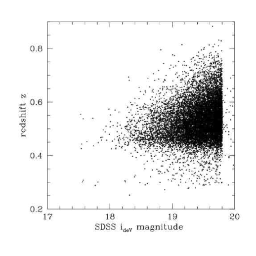
Figure 11: A plot of redshift against $i$-band magnitude for 11,000 2SLAQ galaxies (Samples 8 and 9). The upper diagonal boundary represents the most luminous galaxies at each redshift; the lower boundary at $z\sim 0.45$ is set by the colour selection criteria.

8.2 2-colour distributions for different redshift ranges

The colour distribution of the targets varies strongly as a function of redshift. This is illustrated in Fig. 12 for the primary (Sample 8) data. Each panel is for a different redshift bin in steps of 0.05 in $z$, apart from the low and high-$z$ tails.

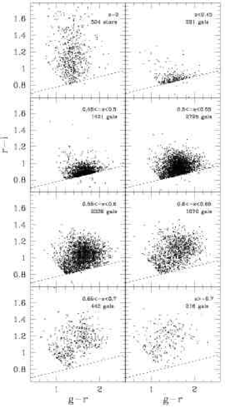
Figure 12: The distribution of LRGs in the 2-colour $(r-i)$ versus $(g-r)$ diagram as a function of $z$, for the primary (Sample 8) objects. Each panel is for a successively larger redshift range, starting with the M-type stars at top left and ending with the highest redshift objects at bottom right. The dotted line in each panel is the $d_{\perp}=0.65$ lower boundary to Sample 8, for reference (a few points appear below this line due to revisions of the photometry). The main clump of LRGs moves to redder $r-i$ colours at approximately constant $g-r$ as $z$ increases, as the 4000Å break moves through the $r$–band.

The top left panel shows the M-stars, which mostly occupy a vertical strip with $g-r\sim 1.4$ and extending to very red $r-i$ colours. For the galaxies in the remaining seven panels, the centroid of the main concentration of points moves to higher values of $(r-i)$ at approximately constant $(g-r)$ as redshift increases, due to the 4000Å break moving through the $r$–band. For $z>0.55$ the main concentration of LRGs moves clear of the colour selection boundaries, indicating that the primary LRG sample has high completeness above the $i$–band apparent magnitude limit. Careful analysis of the numbers of SDSS and 2SLAQ LRGs (Wake et al., 2006) shows they have almost identical luminosity functions at $z=0.24$ and $z=0.6$, indicating that most LRGs were formed at higher redshift and are evolving passively. This conclusion is confirmed by the composite LRG spectra for different redshift ranges presented by Roseboom et al. (2006): these are all very similar to the spectrum of a nearby giant elliptical galaxy such as NGC 3379 (Template 2, Fig. 17) and show only slight evolution for $0.2<z<0.7$.

The 2-colour distribution in Fig. 12 becomes more diffuse as $z$ increases, which may be an indication of increasing levels of current or recent star formation affecting the colours at higher redshifts. However, the errors in the colours also become significant for the faintest and reddest objects, especially in the $g$-band. Objects with $\sigma_{g}>0.35$ have not been plotted, following the discussion of photometric errors in Section 2.1. Such a cut eliminates 3% of the primary sample, including virtually all objects with $(g-r)>2.3$.

8.3 The highest redshift galaxies

For $z>0.55$ the colour distribution appears to be bi-modal, with a clump centred near $(g-r)=1.7$ and a second population towards the lower left corner of each plot, truncated on the blue side by the $c_{\parallel}>1.6$ diagonal limit (cf. Fig. 1). This bimodality is shown more clearly in Fig. 13, a histogram of the distribution of $c_{\parallel}$ for galaxies in the two highest redshift bins from Fig. 12. Further evidence for the reality of this division comes from the distribution of galaxies with strong [O II] emission, as detected during the redshifting process and indicated by the dotted histogram in Fig. 13. The em-line galaxies are strongly concentrated towards the blue boundary. The equivalent widths of the emission lines are not large enough to cause the colour shift directly in true LRGs: it appears most likely that the ‘bluer’ objects represent later-type galaxies with recent star formation, spilling into the 2SLAQ sample from below the colour selection boundaries. Roseboom et al. (2006) and Wake et al. (2006) discuss this effect in some detail, since it has to be corrected for in determining the luminosity functions of the LRGs and in measuring the evolution in the rate of star formation with redshift.

The fraction of emission line galaxies becomes particularly high for the highest redshift group, with $z>0.7$. This is evidence for higher rates of activity (either star-forming or AGN) at earlier epochs, although the statistics have to be corrected for observational selection since the useful spectral range is short and affected by telluric features (see Fig. 6(e)). Sometimes such galaxies can only be assigned reliable redshifts when [O II] 3727Å is present, so there is a bias towards recognising the more active galaxies at high redshift.

Figure 13: A histogram of the distribution of the $c_{\parallel}$ photometric parameter for galaxies in the primary LRG sample with $z\geq 0.65$ and $\sigma_{g}<0.35$. The full line is for all LRGs, the dotted line is for those with [O II] emission. The sharp boundary at $c_{\parallel}=1.6$ marks the LRG colour selection cut-off. The bins are independent, supporting the reality of the dip in the full distribution at $c_{\parallel}=2$. The highly skewed distribution of emission line galaxies indicates the existence of two separate populations of high redshift galaxies, with only the redder peak corresponding to true LRGs.

The template statistics given in Appendix B support the identification of two types of galaxy among the highest redshift 2SLAQ LRGs. The main (redder) concentration of galaxies nearly all fit the composite LRG spectrum (T1) best and must be true LRGs, while many of the bluer galaxies lying close to the $c_{\parallel}$ boundary are best fit by the later-type emission-line galaxy NGC 5248 (T3) (see Fig. 18). The appearance of emission-line or star forming galaxies along the $c_{\parallel}$ boundary is evident in the lower redshift bins as well, at least down to $z>0.4$, which probably indicates that the two basic populations occur throughout the present sample as in other galaxy redshift surveys. This population is a contaminant in the LRG sample, and has to be distinguished from the subset of true LRGs which have emission lines due to either transient star formation or AGN activity, as discussed by Roseboom et al. (2006).

8.4 The ‘failed redshift’ objects

The two-colour distribution of the primary targets which were observed but failed to yield a reliable redshift is shown in Fig. 14. This distribution is not the same as for the full input sample (Fig. 1) or any of the redshift subsamples in Fig. 12. Evidently the redshift failure rate is a complex function of redshift itself, and of other parameters such as magnitude and colour. Fig. 14 suggests that a considerable fraction of the ‘failed’ objects are high redshift galaxies with $z>0.7$, while there is also a significant population near the $d_{\perp}=0.6$ cut-off with colours similar to $z<0.4$ galaxies. There are few failed redshift targets within the main clump of $z\sim 0.55$ LRGs seen in the central panels of Fig. 12, despite these being the dominant population in the sample, indicating that the identification of the true passive LRGs is very nearly complete.

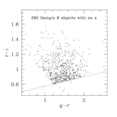
Figure 14: The 2-colour distribution of the 8% of primary (Sample 8) LRGs with unreliable redshifts, i.e. with redshift quality $Q<3$ (again omitting data with $\sigma_{g}>0.35$). This distribution is significantly different from that of the full sample or any of the redshift sub-samples plotted in Fig. 12. A relatively high proportion of objects with extreme colours fail to give good redshifts, while bona fide LRGs in the clump with $z\sim 0.55$ are under-represented. The ‘failed redshift’ objects include a mixture of high redshift galaxies, galaxies with peculiar spectra, composite objects, lower redshift galaxies which are not LRGs, and LRGs which simply had weak spectra because of bad fibre placement or low throughput.

The overall distribution of the failed redshifts shows no significant dependence on apparent $i$-band magnitude or on the general quality of the datasets, as measured by redshift completeness or mean S/N (Section 5.4). Quantitatively, the fraction of failed redshift objects with colours within the main concentration of LRGs (taken here as the objects with $1.4<g-r<1.8,0.9<r-i<1.2$) is only 5% compared with 8% for all objects in Sample 8. By contrast, 12% of the reddest objects with $r-i>1.2$ fail to yield reliable redshifts and this fraction rises to 17% for the bluest objects with $g-r<1.2$.

These variations demonstrate that there are real correlated differences in colour and spectral type within the primary sample: they cannot simply be due to either poor spectra or photometric errors. Many of the reddest and bluest objects must have spectra which are not so well matched to any of the template spectra as are the bulk of the LRGs. Some may be active galaxies of various types, some may be composite spectra due to chance alignments. The ‘failed redshift’ list may also include some very high redshift objects with $z\geq 0.8$, given that such objects are difficult to recognise in the 2SLAQ data. A few spectra with high S/N also fail to yield redshifts; in at least one case this was due to contamination of the spectrum by light from a nearby bright star with an almost featureless spectrum in the 2SLAQ wavelength range.

8.5 Completeness of the 2SLAQ samples

The discussions of the colour distributions above, of sample completeness in Section 5.5 and of redshift reliability in Section 6, together indicate that the 2SLAQ sample of true passively evolving LRGs is over 95% spectroscopically complete and reliable for redshifts between 0.5 and 0.65. Few LRGs can have been missed, and few non-LRGs included, down to the $i_{\rm deV}=19.8$ magnitude limit. The primary Sample 8 is also almost spatially complete in the most fully observed regions, assuming that the SDSS input catalogue is itself almost complete, so that it should be possible to define a sample of LRGs with an absolute completeness of better than 90%.

The primary Sample 8 2SLAQ LRGs therefore provide a good sample of co-moving test particles for cosmological purposes and for constraining LRG evolution. In particular, most of the LRGs seen at redshift 0.65 must be the progenitors of LRGs at $z=0.5$, and of the passively evolving LRGs seen at lower redshift in other surveys.

The secondary Sample 9 2SLAQ LRGs are much less useful for studying large scale structure, since their spatial completeness is very variable from field to field. However, this sample has a much tighter colour distribution than Sample 8 (Fig. 1) and so comprises a more homogeneous set of galaxies, with high redshift completeness and little contamination, which will be very useful for studying the evolution of LRGs.

8.6 The spatial distribution of 2SLAQ LRGs

A map of the spatial distribution of the LRGs within the more complete northern slice is shown in Fig. 15, a plot of redshift (or co-moving radial distance, assuming $\Omega_{m}=0.3$, $\Omega_{\Lambda}=0.7$ and $H_{0}=70$ km s^-1 Mpc^-1) against RA along the equatorial strip. The 2SLAQ LRGs are plotted as large black dots and lie in discrete sectors corresponding to the sub-strips with the best SDSS photometry. The distribution appears non-random with higher density clumps and filaments and lower density voids. The thin pencil-beam extensions down to $z=0.3$ come from the 2dF fields observed early in 2003, using lower-redshift selection criteria. The grey points with $0.25<z<0.5$ are the SDSS LRGs which lie within the same $2\degr$-wide equatorial strip (Eisenstein et al., 2001) and the fine structure with $z<0.2$ comes from a combination of the SDSS MAIN (Strauss et al., 2002) and 2dFGRS (Colless, Dalton, Maddox et al., 2001) galaxies of all types, also within the same narrow strip. The apparently finer structure seen at low redshifts is mainly an artefact of the much higher surface density of points available. This wedge plot gives an excellent impression of how the four surveys complement each other in terms of redshift and spatial coverage. The redshift histogram shown previously as Fig. 10 is effectively a projection of Fig. 15 along the redshift axis.

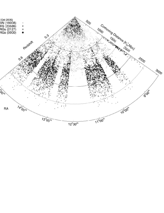
Figure 15: A wedge diagram plotting redshift or distance as a function of RA for all the 2SLAQ LRGs in the Northern Galactic strip (large black points in discrete sectors). Very small points with $z<0.3$ show the 2dFGRS and SDSS MAIN galaxies of all types and the grey points at intermediate redshifts are from the SDSS LRG survey, all lying within the same $2\degr$-wide strip. Considerable structure is evident within the LRG samples, similar to what is seen at much lower redshifts.

The large-scale structure in the 2SLAQ LRGs can be seen more clearly at higher magnification. Fig. 16 is an enlargement of part of Fig. 15 corresponding to sub-strip ‘d’, one of the largest areas with contiguous coverage. A pattern of voids and super-clusters linked by filaments or walls becomes apparent, on the same $\sim 100$ Mpc scales as seen at $z\sim 0.1$ in surveys such as the 2dFGRS (Pimbblet, Drinkwater, & Hawkrigg, 2004) and SDSS MAIN survey (Pandey & Bharadwaj, 2005).

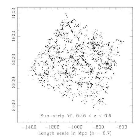
Figure 16: An enlarged portion of Fig. 15 for sub-strip ‘d’ at RA$\sim 14$h. This shows the spatial distribution of 1737 LRGs in the primary and secondary 2SLAQ samples (Samples 8 and 9) with $0.45<z<0.6$. A pattern of voids and super-clusters linked by filaments or walls is apparent, on scales of hundreds of Mpc.

9 Summary

The primary objective of the 2SLAQ LRG survey, to obtain redshifts for more than 10,000 galaxies with $0.45<z<0.7$, has been achieved. The galaxies lie in two thin sectors or wedges, one in each Galactic hemisphere, corresponding to narrow strips running along the celestial equator. The input target selection was based on SDSS $gri$ photometry and has proved to be very efficient with more than 90% of the galaxies falling in the desired high redshift range. More than two thirds of the galaxies are in the northern slice. Reliable redshifts have been obtained for 92% of the objects observed. A large-scale structure of clumps, filaments and voids is apparent in the most complete regions, similar to what was seen in earlier large surveys at lower redshift.

Two thirds of the galaxies are in the photometrically well-defined primary sample and most of the rest (27%) in the secondary sample. The primary sample has high spectroscopic completeness in the sense that good redshifts have been obtained for $\sim 90$% of the targets within the best-observed fields. The survey also has high absolute completeness for LRGs with $z>0.5$ and de-reddened total $i$-band magnitude brighter than 19.6, since such galaxies lie well clear of the photometric selection boundaries. The SDSS-2dF LRG survey thus offers a significant advance in our understanding of the most massive galaxies over the past 8 Gyr: the census of such objects must be almost complete. It should be possible to distinguish unambiguously between continuing hierarchical (i.e. merger) and early (high redshift) models for the formation of LRGs.

For the immediate future, the success of 2SLAQ shows that the new AAOmega spectrograph for 2dF, which gives a gain of a factor of up to four in throughput together with better quality and higher resolution, can be used for cosmological surveys targetting either higher redshifts or much larger samples, or both.

ACKNOWLEDGEMENTS

We particularly thank all members of the AAO staff who helped to run and maintain 2dF, and its complex software, during the course of the 2SLAQ survey.

The 2SLAQ surveys were conducted by a substantial team of people, coordinated by RCN with ACE and MJD as Principal Investigators for the LRGs in the UK and Australia respectively. RDC wishes to acknowledge their crucial roles, and can claim credit only for contributing to the observing and data analysis. He also thanks Will Sutherland and Will Saunders for helpful discussions about the Zcode redshifting software.

ACE acknowledges support through the Royal Society. KAP acknowledges support through an EPSA University of Queensland Research Fellowship and a UQRSF grant. RDC is grateful for the hospitality of the Department of Astrophysics at Oxford, where the final version of this paper was completed.

Funding for the creation and distribution of the SDSS archive has been provided by the Alfred P. Sloan Foundation, the Participating Institutions, NASA, NSF, the US Department of Energy, the Japanese Monbukagakusho, and the Max Planck Society. The SDSS Web site is http://www.sdss.org.

The SDSS is managed by the Astrophysical Research Consortium for the Participating Institutions. The Participating Institutions are the University of Chicago, Fermilab, the Institute for Advanced Study, the Japan Participation Group, The Johns Hopkins University, Los Alamos National Laboratory, the Max-Planck-Institute for Astronomy, the Max-Planck-Institute for Astrophysics, New Mexico State University, the University of Pittsburgh, Princeton University, the United States Naval Observatory, and the University of Washington.

Appendix A 2dF fields and datasets

Data were obtained for 80 discrete 2dF fields during the 2SLAQ survey, some with two or more sets of observations. In general, data obtained in different observing runs have been treated as independent datasets, since the target lists were usually modified between runs. A total of 104 datasets are listed in Table 3.

The first seven columns give the name and centre of each field (equinox J2000). Column 8 identifies each discrete dataset by field name and date, usually in the format YYMMXX: these are the datasets identified in the final redshift catalogues for individual objects (the ‘g’ distinguishes galaxies from QSOs, while the final ‘2’ denotes the spectrograph, in practice always no. 2 for the LRGs). Most fields were observed on two or more nights during an observing run and all the data combined, in which case the final two characters are either ‘00’ or ‘fi’. Occasionally data were obtained on only one night, in which case the last two digits give the date. A few specially combined datasets are identified by other character combinations. Where the same field was observed in different runs the datasets are listed separately since the target lists will be different, although often with many objects in common.

Column 9 gives the number of exposures combined in each dataset, $N_{\mathrm{exp}}$, normally each of 30 min duration. Column 10 gives the mean S/N achieved, averaged over all pixels for all targets, and $D_{\mathrm{mag}}$ in column 11 is the mean offset in magnitudes in a plot of log(counts) versus $r$-band fibre magnitude for each dataset (total $i_{\rm deV}$ magnitude was used instead of $r_{\rm fib}$ for some early datasets: these account for most of the negative values of Dmag). Both of these are indicators of quality. The final three columns give the number of objects in each dataset, the number for which reliable ($Q>2$) redshifts were obtained and the proportion these are of the total. The observations of a field were normally deemed to be complete when the proportion of reliable redshifts was at least 85% (strictly, this criterion was applied to the original set of targets if some fibres were re-allocated after the first night, but the numbers quoted here apply to the full datasets). The footnotes give further details on some datasets.

Table 3: List of 2dF fields observed.

Field	RA	dec	dataset	$N_{\mathrm{exp}}$	S/N	$D_{\mathrm{mag}}$	obj	$Q>2$	%	Notes
a01	08 14 00	$-$00 12 35	a01g_030300_2	12	6.90	$-$0.47	170	159	94	1,2
a02	08 18 00	$-$00 12 35	a02g_033400_2	7	7.22	$-$0.94	165	157	95	1,2,3
a13	09 10 48	$-$00 12 35	a13g_050300_2	9	3.40	0.66	200	166	83
a14	09 15 36	$-$00 12 35	a14g_0404fi_2	7	4.29	0.66	169	159	94
a15	09 20 24	$-$00 12 35	a15g_0404fi_2	7	5.27	0.76	178	171	96
a16	09 25 12	$-$00 12 35	a16g_0404fi_2	8	5.01	0.81	168	147	88
a16	09 25 12	$-$00 12 35	a16g_050314_2	8	5.87	1.04	215	209	97
a17	09 30 00	$-$00 12 35	a17g_0403fi_2	8	5.53	$-$0.91	195	186	95
b01	10 01 00	$-$00 12 35	b01g_030400_2	8	6.63	$-$0.41	142	139	98	2
b00	10 02 00	$-$00 12 35	b00g_050417_2	4	1.67	0.15	172	127	74	4,5
b02	10 05 00	$-$00 12 35	b02g_030300_2	8	7.25	$-$0.86	163	152	93	1,2
b02	10 05 00	$-$00 12 35	b02g_0504fi_2	7	2.00	0.44	188	136	74	5
b03	10 09 00	$-$00 12 35	b03g_030300_2	12	6.74	$-$0.24	166	152	92	1,2
b03	10 09 00	$-$00 12 35	b03g_0504fi_2	8	3.91	0.84	191	173	91
b04	10 13 48	$-$00 12 35	b04g_0403fi_2	8	5.64	$-$0.90	165	158	96
b05	10 18 36	$-$00 12 35	b05g_0404fi_2	8	5.05	0.91	167	153	92
b06	10 23 24	$-$00 12 35	b06g_0403fi_2	8	4.70	1.00	164	151	92
b06	10 23 24	$-$00 12 35	b06g_0504fi_2	7	4.43	0.88	219	198	90
b07	10 28 12	$-$00 12 35	b07g_0404fi_2	9	5.56	1.23	160	157	98
b08	10 33 00	$-$00 12 35	b08g_0404fi_2	11	4.92	1.26	171	159	93
b09	10 37 48	$-$00 12 35	b09g_0503fi_2	11	5.12	1.51	201	184	92
b10	10 42 36	$-$00 12 35	b10g_0404fi_2	8	3.81	0.84	156	142	91
b11	10 47 24	$-$00 12 35	b11g_0503fi_2	8	4.60	1.00	206	197	96
b12	10 52 12	$-$00 12 35	b12g_0504fi_2	13	4.70	1.40	207	190	92
b13	10 57 00	$-$00 12 35	b13g_050400_2	10	5.13	1.20	189	166	88
b14	11 01 48	$-$00 12 35	b14g_050467_2	8	4.66	0.85	183	171	93
b15	11 06 36	$-$00 12 35	b15g_0504fi_2	10	3.79	0.83	187	161	86
b16	11 11 24	$-$00 12 35	b16g_0504fi_2	5	4.71	1.10	209	193	92
c01	12 21 30	$-$00 12 35	c01g_030300_2	8	5.25	$-$0.62	157	143	91	1,2
c00	12 22 30	$-$00 12 35	c00g_0505fi_2	8	4.04	0.92	196	186	95	4
c02	12 25 30	$-$00 12 35	c02g_030300_2	8	6.87	$-$0.90	168	159	95	1,2
c03	12 29 30	$-$00 12 35	c03g_030400_2	8	5.65	$-$0.91	144	130	90	2
c03	12 29 30	$-$00 12 35	c03g_050413_2	4	4.29	0.36	168	152	90
c04	12 33 30	$-$00 12 35	c04g_030400_2	8	6.98	$-$0.67	144	141	98	2
c05	12 38 18	$-$00 12 35	c05g_0403fi_2	10	4.93	$-$1.00	158	147	93
c06	12 43 06	$-$00 12 35	c06g_0404rc_2	15	4.69	1.17	174	151	87
c07	12 47 54	$-$00 12 35	c07g_0403fi_2	9	4.62	0.88	173	164	95
d03	13 12 00	$-$00 12 35	d03g_040422_2	4	3.73	0.21	156	142	91
d04	13 16 48	$-$00 12 35	d04g_0503fi_2	10	4.24	0.96	203	194	96
d05	13 21 36	$-$00 12 35	d05g_0404fi_2	7	3.98	0.70	173	149	86
d06	13 26 24	$-$00 12 35	d06g_0403fi_2	11	5.12	$-$0.79	169	163	96
d07	13 31 12	$-$00 12 35	d07g_0404fi_2	7	3.34	0.41	161	113	70
d07	13 31 12	$-$00 12 35	d07g_0504fi_2	9	5.15	1.15	207	192	93
d08	13 36 00	$-$00 12 35	d08g_030406_2	5	6.68	$-$1.17	165	165	100	2
d08	13 36 00	$-$00 12 35	d08g_0505fi_2	8	5.28	1.05	205	201	98
d09	13 40 00	$-$00 12 35	d09g_030300_2	16	5.60	$-$0.22	165	153	93	1,2,6
d10	13 40 00	$-$00 12 35	d10g_030400_2	11	6.03	$-$0.31	166	163	98	2,6
d10	13 40 00	$-$00 12 35	d10g_0504fi_2	9	3.83	0.76	193	170	88	6
d11	13 44 48	$-$00 12 35	d11g_050467_2	9	4.31	0.95	186	168	90
d12	13 49 36	$-$00 12 35	d12g_0504fi_2	10	3.76	0.84	231	172	74	7
d13	13 54 24	$-$00 12 35	d13g_0503fi_2	8	7.27	1.08	190	175	92
d14	13 59 12	$-$00 12 35	d14g_0404fi_2	6	3.09	0.55	155	107	69
d14	13 59 12	$-$00 12 35	d14g_0504fi_2	10	3.91	0.92	201	182	91
d15	14 04 00	$-$00 12 35	d15g_0503fi_2	7	4.26	1.02	197	176	89
d16	14 08 48	$-$00 12 35	d16g_0404rc_2	12	4.80	1.41	176	160	91
d17	14 13 36	$-$00 12 35	d17g_0503fi_2	12	4.93	1.29	180	172	96
e01	14 34 00	$-$00 12 35	e01g_030400_2	8	4.37	$-$1.18	147	138	94	2
e01	14 34 00	$-$00 12 35	e01g_050411_2	4	3.99	0.37	165	155	94
e02	14 38 00	$-$00 12 35	e02g_030406_2	4	4.65	$-$1.55	156	130	83	2
e02	14 38 00	$-$00 12 35	e02g_050413_2	5	3.51	0.45	143	134	94
e03	14 42 48	$-$00 12 35	e03g_050400_2	15	4.12	1.28	197	182	92
e04	14 47 36	$-$00 12 35	e04g_0404fi_2	11	3.81	0.94	166	145	87
e04	14 47 36	$-$00 12 35	e04g_0505fi_2	7	4.33	0.83	214	194	91
e05	14 52 24	$-$00 12 35	e05g_0504fi_2	10	4.25	1.11	184	165	90

Table 4: continued

Field	RA	dec	dataset	$N_{\mathrm{exp}}$	S/N	$D_{\mathrm{mag}}$	obj	$Q>2$	%	Notes
e06	14 57 12	$-$00 12 35	e06g_0404fi_2	9	3.94	0.93	154	121	79
e06	14 57 12	$-$00 12 35	e06g_0504fi_2	9	3.72	0.91	196	167	85
e07	15 02 00	$-$00 12 35	e07g_050508_2	4	3.21	0.17	169	129	76
e07	15 02 00	$-$00 12 35	e07g_050730_2	8	3.97	0.94	231	209	90
e08	15 06 48	$-$00 12 35	e08g_050417_2	5	2.73	0.16	170	136	80	7
e08	15 06 48	$-$00 12 35	e08g_050802_2	10	4.03	1.02	219	184	84
e09	15 11 36	$-$00 12 35	e09g_050730_2	6	3.39	0.49	198	150	76
e10	15 16 24	$-$00 12 35	e10g_050801_2	7	3.62	0.63	171	145	85
s01	20 57 36	$-$00 15 00	s01g_030800_2	4	2.98	$-$0.47	170	95	56	8,9
s06	21 21 36	$-$00 15 00	s06g_030900_2	12	5.53	0.58	171	155	91
s07	21 26 24	$-$00 15 00	s07g_0410fc_2	10	3.43	0.53	187	159	85
s07	21 26 24	$-$00 15 00	s07g_050730_2	9	3.83	0.69	206	169	82
s08	21 31 12	$-$00 15 00	s08g_04se69_2	18	4.07	$-$1.10	187	148	79
s09	21 36 00	$-$00 15 00	s09g_041013_2	3	2.20	$-$0.54	152	81	53
s09	21 36 00	$-$00 15 00	s09g_050801_2	8	4.38	0.84	166	156	94
s10	21 40 48	$-$00 15 00	s10g_050508_2	3	2.25	$-$0.20	172	111	65
s10	21 40 48	$-$00 15 00	s10g_050729_2	7	2.86	0.51	187	139	74
s11	21 45 36	$-$00 15 00	s11g_050731_2	9	3.61	0.94	204	167	82
s12	21 50 24	$-$00 15 00	s12g_030800_2	13	4.94	0.11	168	152	90	8
s25	22 52 48	$-$00 15 00	s25g_030800_2	14	6.24	0.73	169	163	96	8
s25	22 52 48	$-$00 15 00	s25g_030920_2	4	2.86	$-$0.93	166	135	81
s26	22 57 36	$-$00 15 00	s26g_041013_2	4	2.80	0.04	148	119	80
s26	22 57 36	$-$00 15 00	s26g_050801_2	4	3.25	0.14	164	130	79
s27	23 02 24	$-$00 15 00	s27g_030900_2	8	3.79	$-$0.09	166	148	89
s28	23 07 12	$-$00 15 00	s28g_04oc89_2	11	3.17	0.71	147	122	83
s29	23 12 00	$-$00 15 00	s29g_04com1_2	22	4.17	$-$0.61	169	147	87
s30	23 16 48	$-$00 15 00	s30g_0410fi_2	10	3.45	0.64	170	156	92
s31	23 21 36	$-$00 15 00	s31g_050730_2	8	3.97	0.92	187	169	90
s32	23 26 24	$-$00 15 00	s32g_050801_2	8	3.99	0.76	187	161	86
s47	00 38 24	$-$00 15 00	s47g_050801_2	4	2.88	0.08	187	150	80
s48	00 43 12	$-$00 15 00	s48g_046nts_2	22	3.24	$-$1.06	204	182	89
s49	00 48 00	$-$00 15 00	s49g_041013_2	4	2.69	$-$0.24	158	134	85
s50	00 52 48	$-$00 15 00	s50g_030800_2	12	5.93	0.58	167	158	91	8
s50	00 52 48	$-$00 15 00	s50g_030920_2	4	2.91	$-$0.81	172	143	83
s51	00 57 36	$-$00 15 00	s51g_0410fi_2	12	3.52	0.64	190	168	88
s52	01 02 24	$-$00 15 00	s52g_030900_2	12	4.43	0.21	172	155	90
s67	02 14 24	$-$00 15 00	s67g_040000_2	23	3.95	$-$0.73	162	140	86
s68	02 19 12	$-$00 15 00	s68g_041013_2	4	2.36	0.04	148	121	82
s69	02 24 00	$-$00 15 00	s69g_030900_2	11	4.44	0.21	165	141	85
s70	02 28 48	$-$00 15 00	s70g_0410fi_2	13	3.44	0.77	172	149	87

Notes to Table A1

1. A central wavelength of 6350Å was used in March 2003 for fields a01, a02, b02, b03, c01, c02 and d09. All subsequent data used

6150Å.

2. The target selection in March and April 2003 had an $i_{\rm deV}$ magnitude limit of 19.5. This applies to the fields listed in note 1 plus

b01, c03, c04, d08, e01 and e02. Most of these fields were re-observed subsequently with the standard $i_{\rm deV}=19.8$ limit. However,

a01 and a02 in particular should be omitted from statistical analyses since they have low primary Sample 8 completeness.

3. The redshifts for a02 come from the combined frame for both months, but for some purposes the separate spectra from March or

April 2003 may be better.

4. b00 and c00 are hybrid field centres, shifted 15 arcmin (1 min in RA) east from b01 and c01 respectively, to increase overlap with

b02 and c02.

5. The April 2005 data for b00 and b02 were badly affected by twilight and moonlight; data from the last night only were used for

most b00 objects.

6. d09 and d10 have the same field centre but a different selection of targets, with many faint objects ($19.5<i_{\rm deV}<20$) in d10.

7. There was bad scattered light halation for d12 and e08 in April 2005; the overall $z$ yield for d12 was lowered by many weak spectra

observed on the final night only.

8. The secondary Sample 9 targets were inadvertently given higher priority than the primary Sample 8 targets for fields s01, s12, s25

and s50 in August 2003. s25 and s50 were re-observed in September 2003 but s01 and s12 have very low Sample 8 completeness.

9. s01 has very low redshift completeness and should be omitted from statistical analyses. This field is at low Galactic latitude and

suffers from significant interstellar extinction and high ($\sim~{}20$%) stellar contamination.

Appendix B The 2SLAQ redshifting procedure

This appendix gives more information specific to the redshifting of the 2SLAQ LRGs, in particular regarding the template spectra.

B.1 The template spectra

Nine template spectra were used to derive redshifts for the LRGs, as listed in Table 5 and plotted in Fig. 17. T1 is a composite LRG spectrum derived from the somewhat lower redshift LRGs found in the SDSS LRG survey (Eisenstein et al., 2003): this gives the best fit to at least 65% of the 2SLAQ sample and a reliable redshift for more than 90%, since it is both well-matched to the data and extends down to 3000Å rest wavelength. The second and third are bright galaxies used for the 2dFGRS, NGC 3379 which is a standard E1 elliptical galaxy and NGC 5248, an S0 with emission lines. The next five templates are representative stars covering the spectral classes A to M, three of them in common with the 2dFGRS. T9 is a composite e(a) spectrum (from Paul Hewett).

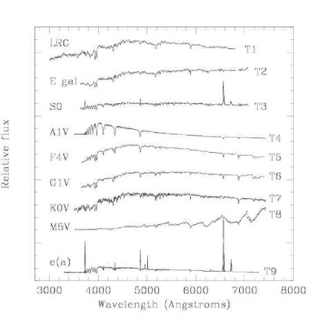
Figure 17: The nine redshift template spectra T1 to T9 from top to bottom, plotted with arbitrary flux scales and offsets. The first and last are composite spectra, the second and third are nearby galaxies, and the remaining five are a sequence of stars from type A to M.

Table 5: The template spectra.

Template	Name	Velocity	$z$	%age
		(km s-1)
T1	lrg_te_s	85	0.50	60.6
T2	NGC3379b	$-$115	0.50	16.2
T3	NGC5248b	$-$90	0.50	8.2
T4	a1star_b	60	0.00	0.3
T5	E323_F4V	85	0.00	2.8
T6	E329_G1V	10	0.00	3.0
T7	k0star_b	$-$130	0.00	0.8
T8	m5star_b	$-$115	0.00	0.0
T9	pch_t1_s	155	0.50	8.1

The third column of Table 5 lists small zero-point velocity offsets which have been derived in two ways: from the mean differences for a set of LRGs, all cross-correlated with each template, and by cross-correlating each template with a synthetic K-type stellar spectrum generated using the ssg code of Bell & Gustafsson (1978). The two techniques gave consistent results to within $\sim 20$ km s^-1, a small error compared with the accuracy of $\sim 100$ km s^-1 for individual galaxy redshifts. These relative velocities are all tied to the composite LRG template T1, whose 85 km s^-1 velocity is the difference between the vacuum wavelengths used by the SDSS and the air wavelengths used by 2dfdr. The effects on the final redshifts are of course small, amounting to no more than 0.0003.

The fourth column of Table 5 is a redshift offset applied to some templates, to optimise the interactive display for most of the targets. The four galaxies were shifted to $z=0.5$, the mean redshift of the LRGs, while the stars were left at $z=0$. The derived redshifts were not affected significantly by these offsets. In practice the only stars which contaminate the LRG sample are M-type dwarfs (5% of the targets), but the G and K-type stellar spectra often provide useful confirmation of the galaxy redshifts, especially for $z<0.4$. The final column in Table 5 gives the percentage of galaxies for which each template was used.

B.2 Usage of templates

The template which gives the best redshift estimate for each galaxy is a function of galaxy type. Fig. 18 shows the redshift distribution for most of the templates. Three of the templates, T4, T7 and T8 for A-, K- and M-type stars respectively, have been omitted because they rarely if ever gave the best fit to a galaxy. Not surprisingly, the mean SDSS LRG spectrum (T1) provides the best fit to by far the largest fraction of the targets, about 60% of the total. The NGC 3379 (T2) spectrum, which is very similar but without the UV tail, was used for a further 16%: for most objects these two templates give virtually identical results. Thus at least three quarters of the 2SLAQ sample matches very well the spectrum of a lower redshift quiescent elliptical galaxy or LRG. Note that the ordinate scales in Fig. 18 are different for these two templates.

Figure 18: Histograms of the redshifts for which each of the templates was used, for Sample 8 and 9 galaxies, omitting the little-used A- and K-type spectra and the M-type spectrum which fitted only foreground M-stars. The numbers of galaxies in each panel are given in parentheses: note the different ordinate scales in the top two panels.

The other two galaxy templates, the emission-line S0 galaxy NGC 5248 (T3) and a ‘k+a+em’ composite (T9), are each used for 8% of the sample. These include a higher proportion of active galaxies, either with active galactic nuclei (AGNs) or star-forming (SF) (these two classes cannot be easily distinguished in the 2SLAQ spectra, since often the only clue is the presence of [O II] at 3727Å), and they tend to be at higher redshifts. Note that the emission lines in T3 and T9 are blanked out for the cross-correlations and do not contribute to the redshift determinations. For the great majority of galaxies with reliable redshifts, all four galaxy templates agree.

The F-, G- and K-type stellar templates together give the best fit to about 6% of the LRGs, although again the galaxy templates usually give the same redshifts. There is a tendency for the stars to be used for the lowest redshift galaxies with $0.3<z<0.4$, perhaps because such galaxies are not true LRGs. The upper cut-off at $z=0.65$ for T5 and T6 is an artefact of the Zcode. The A-type stellar spectrum gives an apparent best fit in only $\sim 0.2$% of cases and is often clearly wrong when the fit is checked visually. The M-type spectrum is used only for foreground M-dwarfs.

References

- Abazajian et al. (2003) Abazajian, K., et al., 2003, AJ, 126, 2081
- Adelman-McCarthy et al. (2006) Adelman-McCarthy, J. K., et al., 2006, ApJSupp, 162, 38
- Bailey, Heald & Croom (2004) Bailey, J. A., Heald, R., Croom, S. M., 2004, The 2dfdr Data Reduction System Users Manual, AAO
- Bell & Gustafsson (1978) Bell R.A., Gustafsson B., 1978, A&AS, 34, 229
- Blake et al. (2006) Blake, C., Collister, A., Bridle, S., Lahav, O., 2006, MNRAS, in press (= astro-ph/0605303)
- Bolton et al. (2004) Bolton, A. S., et al., 2004, AJ, 127, 1860
- Colless, Dalton, Maddox et al. (2001) Colless M. M., Dalton G. B., Maddox S. J., et al., 2001, MNRAS, 328, 1039
- Collister et al. (2006) Collister A., Lahav O., Blake C., et al., 2006, submitted (= astro-ph/06nnnnn)
- Croom et al. (2004) Croom, S. M., Smith, R. J., Boyle, B. J., Shanks, T., Miller, L., Outram, P. J., Loaring, N. S., 2004, MNRAS, 349, 1397
- Croom et al. (2006) Croom, S. M., et al., 2006, in preparation
- Driver et al. (2005) Driver, S. P., Liske, J., Cross, N. J. G., De Propris, R., Allen, P. D., 2005, MNRAS, 360, 81
- Eisenstein et al. (2001) Eisenstein D. J., Annis J., Gunn J. E., Szalay A. S., Connolly A. J., Nichol R. C., et al., 2001, AJ, 122, 2267
- Eisenstein et al. (2003) Eisenstein D. J., et al., 2003, ApJ, 585, 694
- Fukugita et al. (1996) Fukugita, M., et al., 1996, AJ, 111, 1748
- Heavens et al. (2004) Heavens, A., Panter, B., Jimenez, R., Dunlop, J., 2004, Nature, 428, 2474
- Kauffmann et al. (2003) Kauffmann, G., et al., 2003, MNRAS, 341, 54
- Lewis, Cannon, Taylor et al. (2002) Lewis I. J., Cannon R. D., Taylor K., et al., 2002, MNRAS, 333, 279
- Liske et al. (2003) Liske, J., Lemon, D. J., Driver, S. P., Cross, N. J. G., Couch, W. J., 2003, MNRAS, 344, 307
- Padmanabhan et al. (2005) Padmanabhan, N., et al., 2005, MNRAS, 359, 237
- Pandey & Bharadwaj (2005) Pandey B., Bharadwaj S., 2005, MNRAS, 357, 1068
- Pimbblet, Drinkwater, & Hawkrigg (2004) Pimbblet K. A., Drinkwater M. J., Hawkrigg M. C., 2004, MNRAS, 354, L61
- Richards et al. (2005) Richards G. T., et al., 2005, MNRAS, 360, 839
- Roseboom et al. (2006) Roseboom I. et al., 2006, MNRAS submitted
- Ross et al. (2006) Ross, N., et al., 2006, MNRAS in preparation
- Sadler et al. (2006) Sadler, E. M., et al., 2006, MNRAS in preparation
- Schlegel, Finkbeiner & Davis (1998) Schlegel, D. J., Finkbeiner, D.P., & Davis, M., 1998, ApJ, 500, 525
- Spergel et al. (2003) Spergel, D. N., et al., 2003, Ap J Suppl, 148, 175
- Stoughton et al. (2002) Stoughton , C., et al., 2002, AJ, 123, 485
- Strauss et al. (2002) Strauss M. A., Weinberg D. H., Lupton R. H., Narayanan V. K., et al., 2002, AJ, 124, 1810
- Sutherland (1999) Sutherland W. J., 1999, The 2dF Redshift Code - User Guide (available via the AAO)
- Tonry & Davis (1979) Tonry J., Davis M., 1979, AJ, 84, 1511
- Wake et al. (2006) Wake, D., et al., 2006, MNRAS submitted (= astro-ph/06nnnnn)
- York et al. (2000) York, D., et al., 2000, AJ, 120, 1579