Non-Gaussianity of the primordial perturbation in the curvaton model

Abstract

We use the $\delta N$-formalism to investigate the non-Gaussianity of the primordial curvature perturbation in the curvaton scenario for the origin of structure. We numerically calculate the full probability distribution function allowing for the non-instantaneous decay of the curvaton and compare this with analytic results derived in the sudden-decay approximation. We also present results for the leading-order contribution to the primordial bispectrum and trispectrum. In the sudden-decay approximation we derive a fully non-linear expression relating the primordial perturbation to the initial curvaton perturbation. As an example of how non-Gaussianity provides additional constraints on model parameters, we show how the primordial bispectrum on CMB scales can be used to constrain variance on much smaller scales in the curvaton field. Our analytical and numerical results allow for multiple tests of primordial non-Gaussianity, and thus they can offer consistency tests of the curvaton scenario.

I Introduction

Most inflationary models give rise to a nearly Gaussian distribution of the primordial curvature perturbation, $\zeta$. Deviations from an exactly Gaussian distribution are conventionally given in terms of a non-linearity parameter, $f_{\rm{NL}}$ Komatsu and Spergel (2001). The prediction for the non-linearity parameter from single-field models of inflation is related to the tilt of the power spectrum, $f_{\rm{NL}}\sim n-1$ Maldacena (2003) which is constrained by observations to be much less than unity. In principle, measurement of $f_{\rm{NL}}$ would give a valuable test of the inflation, but unfortunately such a tiny non-Gaussianity is likely to remain unobservable. The current upper bound from the WMAP three-year data Spergel et al. (2006) is $|f_{\rm{NL}}|<114$ while Planck is expected to bring this down to $|f_{\rm{NL}}|\lesssim 5$ Komatsu and Spergel (2001) which is still orders of magnitude larger than the prediction for single-field inflation.

On the other hand, multi-field models of inflation can lead to an observable non-Gaussianity. One well-motivated example is the curvaton model Lyth and Wands (2002); Enqvist and Sloth (2002); Moroi and Takahashi (2001): In addition to the inflaton $\phi$ there would be another, weakly coupled, light scalar field (e.g., MSSM flat direction Enqvist et al. (2003); Allahverdi et al. (2006)), curvaton ${\chi}$, which was completely subdominant during inflation. The potential could be as simple as Bartolo and Liddle (2002) $V=\textstyle{\frac{1}{2}}M^{2}\phi^{2}+\textstyle{\frac{1}{2}}m^{2}{\chi}^{2}$, where the energy density of $\phi$ drives inflation. At Hubble exit during inflation both fields acquire some classical perturbations that freeze in. However, the observed cosmic microwave (CMB) and large-scale structure (LSS) perturbations can result from the curvaton instead of the inflaton. If the inflaton mass $M$ is much less than $10^{13}$ GeV then perturbations due to the inflaton are much smaller than $10^{-5}$.

After the end of inflation the inflaton decays into relativistic particles (“radiation”), the curvaton energy density still being subdominant. At this stage the curvaton carries an isocurvature (entropy) perturbation. The entropy perturbation between radiation and curvaton is given by ${\cal S}_{{\chi}}\equiv 3(\zeta_{\chi}-\zeta_{r})$. Observations rule out purely isocurvature primordial perturbations Enqvist et al. (2000, 2002), but, so long as the curvaton decays into radiation before primordial nucleosynthesis, the entropy perturbation can be converted to an adiabatic one. This also requires that all the species are in thermal equilibrium and that the baryon asymmetry is generated after the curvaton decays. If any of these conditions are not met then the curvaton could also leave a residual isocurvature perturbation Lyth et al. (2003), but in practice the amplitude of isocurvature modes are severely constrained by current data Trotta (2006); Lewis (2006); Bean et al. (2006) and for simplicity we will not consider this possibility in this paper.

As the Hubble rate, $H$, decreases with time after inflation, eventually $H^{2}\lesssim m^{2}$, and the curvaton starts to oscillate about the minimum of its potential. Then it behaves like pressureless dust (with density inversely proportional to volume, $\rho_{\chi}\propto a^{-3}$) so that its relative energy density grows with respect to radiation ($\rho_{r}\propto a^{-4}$). Finally, the curvaton decays into ultra-relativistic particles leading to the standard radiation dominated adiabatic primordial perturbations . However, this curvaton mechanism may, from the initially Gaussian curvaton field perturbation, $\delta{\chi}_{\ast}$, create a strongly non-Gaussian primordial curvature perturbation, $\zeta$. The non-Gaussianity is large if the energy density of the curvaton is sub-dominant when curvaton decays. Since the amplitude of the resulting perturbation depends on the model parameters (such as the curvaton mass $m$ and decay rate $\Gamma$), the observational bounds on non-Gaussianity provide important constraints on model parameters.

The objective of this paper is to calculate the probability density function (pdf) of the primordial curvature perturbation in the curvaton model. Since, in the early universe, all today’s observable scales are super-Hubble scales after inflation, we take advantage of the separate universe assumption Sasaki and Tanaka (1998); Wands et al. (2000) throughout the calculations and employ the so-called $\delta N$-formalism Starobinsky (1985); Sasaki and Stewart (1996); Lyth and Rodriguez (2005). This allows us to determine the pdf fully non-linearly (not just up to second or third order in the initial field perturbations) so that it will carry all the information about non-Gaussianity.

Generally we can expand any field

$$\varphi=\bar{\varphi}+\sum_{n=1}^{\infty}\frac{1}{n!}\delta_{n}\varphi\,.$$ (1)

We take the background field to be spatially homogeneous, $\bar{\varphi}(t)$, and we will further assume that the first-order perturbation, $\delta_{1}\varphi(t,x)$ is a Gaussian random field, consistent with what we expect from the linear evolution of initial vacuum fluctuations. Thus the higher-order perturbations, $\delta_{n}\varphi$ for $n>1$, will describe non-Gaussian perturbations of any field.

The primordial perturbation can be described in terms of the non-linear curvature perturbation on uniform-density hypersurfaces Lyth et al. (2005)

$$\zeta(t,{\bf x})=\delta N(t,{\bf x})+\frac{1}{3}\int_{\bar{\rho}(t)}^{\rho(t,{\bf x})}\frac{d\tilde{\rho}}{\tilde{\rho}+\tilde{P}}\,,$$ (2)

where $\delta N$ is the perturbed expansion, $\tilde{\rho}$ the local density and $\tilde{P}$ the local pressure. We expand the curvature perturbation as

$$\zeta(t,{\bf x})=\zeta_{1}(t,{\bf x})+\sum_{n=2}^{\infty}\frac{1}{n!}\zeta_{n}(t,{\bf x})\,,$$ (3)

where the pdf of $\zeta_{1}$ is Gaussian as it is directly proportional to the initial Gaussian field perturbation, but the higher-order terms give rise to a non-Gaussian pdf of the full $\zeta$. The non-linearity parameters $f_{\rm{NL}}$ and $g_{\rm{NL}}$ are defined by

$$\zeta=\zeta_{1}+\frac{3}{5}f_{\rm{NL}}\zeta_{1}^{2}+\frac{9}{25}g_{\rm{NL}}\zeta_{1}^{3}+{\cal O}(\zeta_{1}^{4})\,,$$ (4)

or, equivalently,

$$\zeta_{2} = \frac{6}{5}f_{\rm{NL}}\zeta_{1}^{2}\,,$$ (5)

$$\zeta_{3} = \frac{54}{25}g_{\rm{NL}}\zeta_{1}^{3}\,\,.$$ (6)

The numerical factors $6/5$ and $54/25$ arise because in linear theory the primordial curvature perturbation $\zeta$ is related to the Bardeen potential on large scales (in the matter-dominated era, md), $\Phi_{H\rm md}=(3/5)\zeta_{1}$, which implies Komatsu and Spergel (2001); Okamoto and Hu (2002); Kogo and Komatsu (2006)

$$\frac{3}{5}\zeta=\Phi_{H\rm md}+f_{\rm{NL}}\Phi_{H\rm md}^{2}+g_{\rm{NL}}\Phi_{H\rm md}^{3}\,.$$ (7)

We are specifically interested in non-linear quantities and, as it is $\zeta$ not $\Phi_{H}$ that is non-linearly conserved for adiabatic perturbation on large scales Lyth and Wands (2003); Rigopoulos and Shellard (2003); Malik and Wands (2004); Lyth et al. (2005); Langlois and Vernizzi (2005), we will take Eqs. (5) and (6) as our fundamental definition of the primordial parameters $f_{\rm{NL}}$ and $g_{\rm{NL}}$, respectively.

If we write the primordial power spectrum as

$$\langle\zeta({\bf k_{1}})\zeta({\bf k_{2}})\rangle=(2\pi)^{3}P(k_{1})\delta^{3}({\bf k_{1}}+{\bf k_{2}})\,,$$ (8)

then the leading order contributions to the bispectrum and (connected part of the) trispectrum are given by

$$\langle\zeta( {\bf k_{1}})\zeta({\bf k_{2}})\zeta({\bf k_{3}})\rangle$$ (9)

$$= \!\!(2\pi)^{3}B({\bf k_{1}},{\bf k_{2}})\delta^{3}({\bf k_{1}}+{\bf k_{2}}+{\bf k_{3}})\,,$$

$$\langle\zeta( {\bf k_{1}})\zeta({\bf k_{2}})\zeta({\bf k_{3}})\zeta({\bf k_{4}})\rangle$$ (10)

$$= \!\!(2\pi)^{3}T({\bf k_{1}},{\bf k_{2}},{\bf k_{3}})\delta^{3}({\bf k_{1}}+{\bf k_{2}}+{\bf k_{3}}+{\bf k_{4}}),$$

where

$$B({\bf k_{1}},{\bf k_{2}})\!\! = \!\!(6/5)f_{\rm{NL}}\left[P(k_{1})P(k_{2})+2\,{\rm perms}\right]\!,$$ (11)

$$\!\!\!\!\!T({\bf k_{1}},{\bf k_{2}},{\bf k_{3}})\!\! =$$

$$(18/25)f_{\rm{NL}}^{2} \left[P(k_{1})P(k_{2})P(|{\bf k_{1}}+{\bf k_{2}}|)+23\,{\rm perms}\right]$$

$$+(54/25)g_{\rm{NL}} \left[P(k_{1})P(k_{2})P(k_{3})+3\,{\rm perms}\right]\,.$$ (12)

The first term appearing in Eq. (12), which gives the dependence of the trispectrum on second-order perturbations, and hence $f_{\rm{NL}}$, was given in Boubekeur and Lyth (2006). But there is also a term dependent upon the third-order perturbation, and hence $g_{\rm{NL}}$, which appears at the same order, and has a different dependence upon the four wavevectors.

Previous estimates of non-Gaussianity in the curvaton scenario have been based on expansions up to second order in the curvature perturbation. We will go beyond previous analyses and calculate the contribution of the third order term in Eq. (4) to the trispectrum. We compare our analytic expressions for $f_{\rm{NL}}$ and $g_{\rm{NL}}$ in the sudden-decay approximation Bartolo et al. (2004); Lyth and Rodriguez (2005) with numerical results where we include the gradual decay of the curvaton, transferring energy from the curvaton to the radiation. Indeed using our numerical code we are able for the first time to give the full probability distribution for the primordial curvature perturbation in both the sudden-decay and the non-instantaneous decay case. We will calculate the skewness (third moment of the pdf) and kurtosis (fourth moment of the pdf) as well as higher moments of the fully non-linear probability distribution function.

This paper is organised as follows. In Sec. II we relate the curvaton curvature perturbation $\zeta_{\chi}$ to the initial field perturbation $\delta_{1}{\chi}$ at the beginning of the curvaton oscillation. Then, in Sec.  III, we derive in the sudden-decay approximation a non-linear equation that relates the primordial curvature perturbation $\zeta$ (when curvaton has decayed) to the curvaton curvature perturbation at the beginning of curvaton oscillation, $\zeta_{{\chi}}$, (or to the Gaussian curvaton field perturbation $\delta{\chi}_{\ast}$ at horizon exit). We write down the full solution of this equation in the Appendix A. In Sec. III we continue solving this equation order by order, and deriving the non-linearity parameters $f_{\rm{NL}}$ and $g_{\rm{NL}}$ in the sudden-decay approximation. In Sec. IV we describe our fully non-linear numerical approach. We compare the numerical non-instantaneous decay results for $f_{\rm{NL}}$ and $g_{\rm{NL}}$ to the sudden-decay approximation. In Sec. V we calculate the pdf of $\zeta$ both in the sudden-decay approximation and in the non-instantaneous decay case. We show the skewness and kurtosis of the pdf as a function of curvaton model parameters. In Sec. VI we add one possible complication to the analysis. Namely, the variance of curvaton field perturbations $\langle(\delta{\chi})^{2}/\bar{\chi}^{2}\rangle$ on smaller than observable scales is not directly constrained. However, the large variance leads to large non-Gaussianity (see e.g. Linde and Mukhanov (1997, 2006)) so that the observational bounds on non-Gaussianity set an upper limit to this small-scale variance. We derive a quantitative equation that relates $f_{\rm{NL}}$ and the variance, and use this equation with WMAP third year bounds. Finally, in Sec. VII we present concluding remarks.

II Non-linearity of the curvaton perturbation

When the curvaton starts to oscillate about the minimum of its potential, but before it decays, the non-linear curvature perturbation on uniform-curvaton density hypersurfaces is given by Lyth et al. (2005)

$$\zeta_{\chi}(t,{\bf x})=\delta N(t,{\bf x})+\int_{\bar{\rho}_{\chi}(t)}^{\rho_{\chi}(t,{\bf x})}\frac{d\tilde{\rho}_{\chi}}{3\tilde{\rho}_{\chi}}\,.$$ (13)

Hence, the curvaton density on spatially-flat hypersurfaces is

$$\left.\rho_{\chi}\right|_{\delta N=0}=e^{3\zeta_{\chi}}\bar{\rho}_{\chi}\,.$$ (14)

Assuming the curvaton potential is described by a quadratic potential about its minimum, the energy density is given in terms of the amplitude of the curvaton field oscillations

$$\rho_{\chi}=\frac{1}{2}m^{2}{\chi}^{2}\,.$$ (15)

We expect the quantum fluctuations in a weakly coupled field such as the curvaton at Hubble exit during inflation, $\delta{\chi}_{*}$, to be well described by a Gaussian random field (see e.g. Seery and Lidsey (2005); Lyth and Zaballa (2005); Seery et al. (2006)). Hence we will write

$${\chi}_{*}=\bar{\chi}_{*}+\delta_{1}{\chi}_{*}\,,$$ (16)

with no higher-order, non-Gaussian terms.

Non-linear evolution on large scales is possible if the curvaton potential deviates from a purely quadratic potential away from its minimum Lyth (2004); Enqvist and Nurmi (2005). Thus, in general, the initial amplitude of curvaton oscillations, ${\chi}$, is some function of the field value at the Hubble exit; ${\chi}=g({\chi}_{\ast})$. (The curvaton potential is in any case virtually quadratic sufficiently close to the minimum.) Thus we have during the curvaton oscillation

$$\bar{\rho}_{\chi} = \textstyle{\frac{1}{2}}m^{2}\bar{g}^{2}\,,$$ (17)

$$\rho_{\chi} = \textstyle{\frac{1}{2}}m^{2}\left[\bar{g}+\sum_{n=1}^{\infty}\frac{1}{n!}g^{(n)}\left(\frac{\bar{g}}{g^{\prime}}\frac{\delta_{1}{\chi}}{\bar{\chi}}\right)^{n}\right]^{2}\,,$$ (18)

where we used the relation $\delta_{1}{\chi}=g^{\prime}\delta_{1}{\chi}_{\ast}$ and wrote $\bar{g}\stackrel{{\scriptstyle\mbox{\tiny{def}}}}{{=}}g(\bar{\chi}_{\ast})$ and $g^{(n)}\stackrel{{\scriptstyle\mbox{\tiny{def}}}}{{=}}\left.\partial^{n}g({\chi})/\partial{\chi}^{n}\right|_{{\chi}=\bar{\chi}_{\ast}}$.

Substituting (18) and (17) into (14) we obtain

$$e^{3\zeta_{\chi}} = \frac{1}{\bar{g}^{2}}\left[\bar{g}+\sum_{n=1}^{\infty}\frac{1}{n!}g^{(n)}\left(\frac{\bar{g}}{g^{\prime}}\frac{\delta_{1}{\chi}}{\bar{\chi}}\right)^{n}\right]^{2}\,.$$ (19)

Order by order, we have from (18)

$$\delta_{1}\rho_{\chi} = m^{2}g\delta_{1}{\chi}\,,$$ (20)

$$\delta_{2}\rho_{\chi} = m^{2}\left(1+\frac{gg^{\prime\prime}}{g^{\prime 2}}\right)\left(\delta_{1}{\chi}\right)^{2}\,,$$ (21)

$$\delta_{3}\rho_{\chi} = m^{2}\left(3\frac{g^{\prime\prime}}{g^{\prime 2}}+\frac{gg^{\prime\prime\prime}}{g^{\prime 3}}\right)\left(\delta_{1}{\chi}\right)^{3}\,,$$ (22)

and from (19)

$$\zeta_{{\chi}1} = \frac{2}{3}\frac{\delta_{1}{\chi}}{\bar{\chi}}\,,$$ (23)

$$\zeta_{{\chi}2} = -\frac{3}{2}\left(1-\frac{gg^{\prime\prime}}{g^{\prime 2}}\right)\zeta_{{\chi}1}^{2}$$ (24)

$$\zeta_{{\chi}3} = \frac{9}{2}\left(1-\frac{3}{2}\frac{gg^{\prime\prime}}{g^{\prime 2}}+\frac{1}{2}\frac{g^{2}g^{\prime\prime\prime}}{g^{\prime 3}}\right)\zeta_{{\chi}1}^{3}\,.$$ (25)

Here and in what follows, we omit the bar from $\bar{g}$ and simply denote it by $g$.

Using (23) and (24), we can express the second-order skewness in terms of the effective non-linearity parameter for the curvaton perturbation, analogous to Eq. (5),

$$f_{\rm{NL}}^{{\chi}}=-\frac{5}{4}\left(1-\frac{gg^{\prime\prime}}{g^{\prime 2}}\right)\,.$$ (26)

Hence we find $f_{\rm{NL}}^{\chi}=-5/4$ for the curvaton $\zeta_{\chi}$ in the absence of any non-linear evolution ($g^{\prime\prime}=0$). If the curvaton comes to dominate the total energy density in the universe before it decays, so that $\zeta=\zeta_{\chi}$, then this is the generic prediction for the primordial $f_{\rm{NL}}$ in the curvaton model, as emphasised by Lyth and Rodriguez (2005).

From the third-order term (25) we obtain a contribution to the trispectrum of the curvaton perturbation, described by a non-linearity parameter analogous to Eq. (6),

$$g_{\rm{NL}}^{{\chi}}=\frac{25}{12}\left(1-\frac{3}{2}\frac{gg^{\prime\prime}}{g^{\prime 2}}+\frac{1}{2}\frac{g^{2}g^{\prime\prime\prime}}{g^{\prime 3}}\right)\,.$$ (27)

III Sudden-decay approximation

Most analytic expressions for the primordial density perturbation in the curvaton scenario assume the instantaneous decay of the curvaton particles. In this section we will derive an equation for the non-linear curvature perturbation, and then use it to find the non-linearity parameters $f_{\rm{NL}}$ and $g_{\rm{NL}}$ in this sudden-decay approximation.

In the absence of interactions, fluids with a barotropic equation of state, such as radiation ($P_{r}=\rho_{r}/3$) or the non-relativistic curvaton ($P_{\chi}=0$), have a conserved curvature perturbation Lyth et al. (2005)

$$\zeta_{i}=\delta N+\frac{1}{3}\int_{\bar{\rho}_{i}}^{\rho_{i}}\frac{d\tilde{\rho}_{i}}{\tilde{\rho}_{i}+P_{i}(\tilde{\rho}_{i})}\,.$$ (28)

We assume that the curvaton decays on a uniform-total density hypersurface corresponding to $H=\Gamma$, i.e., when the local Hubble rate equals the decay rate for the curvaton (assumed constant). Thus on this hypersurface we have

$$\rho_{r}(t_{\rm dec},{\bf x})+\rho_{\chi}(t_{\rm dec},{\bf x})=\bar{\rho}(t_{\rm dec})\,,$$ (29)

where we use a bar to denote the homogeneous, unperturbed quantity. Note that from Eq. (2) we have $\zeta=\delta N$ on the decay surface, and we can interpret $\zeta$ as the perturbed expansion, or “$\delta N$”. Assuming all the curvaton decay products are relativistic, we have that $\zeta$ is conserved after the curvaton decay since the total pressure is simply $P=\rho/3$.

By contrast the local curvaton and radiation densities on this decay surface may be inhomogeneous and we have from Eq. (28)

$$\zeta_{r} = \zeta+\frac{1}{4}\ln\left(\frac{\rho_{r}}{\bar{\rho}_{r}}\right)\,,$$ (30)

$$\zeta_{\chi} = \zeta+\frac{1}{3}\ln\left(\frac{\rho_{\chi}}{\bar{\rho}_{\chi}}\right)\,,$$ (31)

or, equivalently,

$$\rho_{r} = \bar{\rho}_{r}e^{4(\zeta_{r}-\zeta)}\,,$$ (32)

$$\rho_{\chi} = \bar{\rho}_{\chi}e^{3(\zeta_{\chi}-\zeta)}\,.$$ (33)

Requiring that the total density is uniform on the decay surface, Eq. (29), then gives the relation

$$(1-\Omega_{{\chi},{\rm{dec}}})e^{4(\zeta_{r}-\zeta)}+\Omega_{{\chi},{\rm{dec}}}e^{3(\zeta_{\chi}-\zeta)}=1\,,$$ (34)

where $\Omega_{{\chi},{\rm{dec}}}=\bar{\rho}_{\chi}/(\bar{\rho}_{r}+\bar{\rho}_{\chi})$ is the dimensionless density parameter for the curvaton at the decay time. This simple equation is one of the main results of this paper. It gives a fully non-linear relation between the primordial curvature perturbation, $\zeta$, which remains constant on large scales in the radiation-dominated era after the curvaton decays, and the curvaton perturbation, $\zeta_{\chi}$ described in Sec. II, in the sudden-decay approximation. In the limiting case where $\Omega_{{\chi},{\rm{dec}}}\to 1$ (i.e., the energy density of the curvaton comes to dominate before it decays) we have $\zeta\to\zeta_{\chi}$, but in general Eq. (34) gives a non-linear relation between $\zeta$ and $\zeta_{\chi}$.

For simplicity we will restrict the following analysis to the simplest curvaton scenario in which the curvature perturbation in the radiation fluid before the curvaton decays is negligible, i.e., $\zeta_{r}=0$. After the curvaton decays the universe is dominated by radiation, with equation of state $P=\rho/3$, and hence the curvature perturbation, $\zeta$, is non-linearly conserved on large scales. With $\zeta_{r}=0$ Eq. (34) reads

$$e^{4\zeta}-\left[\Omega_{{\chi},{\rm{dec}}}e^{3\zeta_{\chi}}\right]e^{\zeta}+\left[\Omega_{{\chi},{\rm{dec}}}-1\right]=0\,,$$ (35)

which is a fourth degree equation for $X=e^{\zeta}$. In the Appendix A we give the solution of this equation. Since we already know $e^{3\zeta_{\chi}}$ as a function of the initial field perturbation $\delta{\chi}_{\ast}$, we have now found a full non-linear mapping of the Gaussian perturbation $\delta{\chi}_{\ast}$ to the primordial (non-Gaussian) curvature perturbation $\zeta$. We can Taylor expand the solution (113) to find first, second, and third order expressions or we can (re-)solve Eq. (35) order by order as we do in the following subsections.

III.1 First order

At first order Eq. (34) gives

$$4(1-\Omega_{{\chi},{\rm{dec}}})\zeta_{1}=3\Omega_{{\chi},{\rm{dec}}}(\zeta_{{\chi}1}-\zeta_{1})\,,$$ (36)

and hence we can write

$$\zeta_{1}=r\zeta_{{\chi}1}\,,$$ (37)

where Lyth and Wands (2002)

$$r=\frac{3\Omega_{{\chi},{\rm{dec}}}}{4-\Omega_{{\chi},{\rm{dec}}}}=\left.\frac{3\bar{\rho}_{\chi}}{3\bar{\rho}_{\chi}+4\bar{\rho}_{r}}\right|_{t_{\rm dec}}\,.$$ (38)

III.2 Second order

At second order Eq. (34) gives

$$4(1-\Omega_{{\chi},{\rm{dec}}})\zeta_{2}-16(1-\Omega_{{\chi},{\rm{dec}}})\zeta_{1}^{2}\\ =3\Omega_{{\chi},{\rm{dec}}}(\zeta_{{\chi}2}-\zeta_{2})+9\Omega_{{\chi},{\rm{dec}}}(\zeta_{{\chi}1}-\zeta_{1})^{2}\,,$$ (39)

and hence, using Eqs. (24), (37) and (38),

$$\zeta_{2}=\left[\frac{3}{2r}\left(1+\frac{gg^{\prime\prime}}{g^{\prime 2}}\right)-2-r\right]\zeta_{1}^{2}\,.$$ (40)

This gives the non-linearity parameter (5) in the sudden-decay approximation Bartolo et al. (2004); Lyth and Rodriguez (2005)

$$f_{\rm{NL}}=\frac{5}{4r}\left(1+\frac{gg^{\prime\prime}}{g^{\prime 2}}\right)-\frac{5}{3}-\frac{5r}{6}\,.$$ (41)

In the limit $r\to 1$, when the curvaton dominates the total energy density before it decays, we recover the non-linearity parameter (26) of the curvaton

$$f_{\rm{NL}}\to-\frac{5}{4}\left(1-\frac{gg^{\prime\prime}}{g^{\prime 2}}\right)\,.$$ (42)

On the other hand we may get a large non-Gaussianity ($|f_{\rm{NL}}|\gg 1$) in the limit $r\to 0$ , where we have

$$f_{\rm{NL}}\to\frac{5}{4r}\left(1+\frac{gg^{\prime\prime}}{g^{\prime 2}}\right)\,.$$ (43)

III.3 Third order

At third order we obtain from Eq. (35)

$$\zeta_{3} = \left[\frac{9}{4r^{2}}\left(\frac{{{g}}^{2}{g^{\prime\prime\prime}}}{{g^{\prime}}^{3}}+3\frac{g\,{g^{\prime\prime}}}{{g^{\prime}}^{2}}\right)-\frac{9}{r}\left(1+\frac{g\,{g^{\prime\prime}}}{{g^{\prime}}^{2}}\right)\right.$$ (44)

$$\left.+\frac{1}{2}\left(1-9\frac{g\,{g^{\prime\prime}}}{{g^{\prime}}^{2}}\right)+10r+3r^{2}\right]\zeta_{1}^{3}\,.$$

The non-linearity parameter $g_{\rm{NL}}$ from Eq. (6) will thus be $25/54$ times the expression in the square brackets. (As a consistency check we note that in the limit $r\to 1$ this result agrees with (27).)

If there is non-linear evolution of the curvaton field, ${\chi}$, between Hubble-exit and the start of the curvaton oscillation, such that $gg^{\prime\prime}/{g^{\prime}}^{2}\simeq-1$, then from (41) we see that $f_{\rm{NL}}$ can be small even when $r\to 0$, see also Lyth (2004); Enqvist and Nurmi (2005). However, in this case $g_{\rm{NL}}$ will be very large unless in (44) the $g^{2}g^{\prime\prime\prime}/{g^{\prime}}^{3}$ term also cancels the $3gg^{\prime\prime}/{g^{\prime}}^{2}$ term. Indeed, assuming that the $g^{\prime\prime\prime}$ term is small, we find $\zeta_{3}\to-[27/(4r^{2})]\zeta_{1}^{3}$, i.e., $g_{\rm{NL}}\to-25/(8r^{2})$, when $r\to 0$ if $gg^{\prime\prime}/{g^{\prime}}^{2}\simeq-1$. In this situation $\zeta_{3}$ would be of the same order as $\zeta_{1}\sim 10^{-5}$, if $r\lesssim 10^{-5}$. Hence, even if the non-linear evolution of the ${\chi}$ field was such that the leading order non-Gaussianity, $f_{\rm{NL}}$, was cancelled, the higher order terms could still lead to large non-Gaussianity which could be ruled out by observations.

In the absence of any non-linear evolution of ${\chi}$ field between the Hubble exit and the start of curvaton oscillation (as in the case of truly quadratic potential) we would have $g^{\prime\prime}=g^{\prime\prime\prime}=0$, so the third order result would be simply

$$\zeta_{3} = \left[-\frac{9}{r}+\frac{1}{2}+10r+3r^{2}\right]\zeta_{1}^{3}\,,$$ (45)

$$g_{\rm{NL}} = \frac{25}{54}\left[-\frac{9}{r}+\frac{1}{2}+10r+3r^{2}\right]\,.$$ (46)

It should be noted that now there is no $1/r^{2}$ term in this $g_{\rm{NL}}$. Thus it is only at most of the same order as $f_{\rm{NL}}$. Indeed, in the limit $r\to 0$ we have $f_{\rm{NL}}\to 5/(4r)$ and $g_{\rm{NL}}\to-25/(6r)$, i.e., $g_{\rm{NL}}/f_{\rm{NL}}\to-10/3$. As $\zeta_{1}\simeq 10^{-5}$ this means that, in this case, the third-order term $\zeta_{3}$ is about 5 orders of magnitude smaller than the second-order term $\zeta_{2}$ even when $r\to 0$.

IV Numerical calculation

Although the sudden-decay approximation gives a good intuitive derivation of both the linear curvature perturbation and the non-linearity parameters arising from second- and third-order effects, it is only approximate since it assumes the curvaton is not interacting with the radiation, and hence $\zeta_{\chi}$ remains constant on large scales, right up until curvaton decays. In practice the curvaton energy density is continually decaying once the curvaton begins oscillating until finally (when $\Gamma>H$) its density becomes negligible, and during this decay process $\zeta_{\chi}$ does not remain constant Malik et al. (2003); Gupta et al. (2004).

Another problem with results derived from the sudden-decay approximation is that the final amplitude of the primordial curvature perturbation, and its non-linearity, are given in terms of the density of the curvaton at the decay time which is not simply related to the initial curvaton density, especially as the precise decay time, $H\sim\Gamma$, is ambiguous.

In fact a more careful treatment of the continuous decay of the curvaton Malik et al. (2003); Gupta et al. (2004) shows that the transfer coefficient at first order, $r$ in Eq. (37), is a function solely of the parameter

$$p\equiv\left[\Omega_{\chi}\sqrt{\frac{H}{\Gamma}}\right]_{\rm osc}\,,$$ (47)

where the right hand side is to be evaluated when the curvaton begins to oscillate, long before it decays, and hence can be written as

$$p=\frac{8\pi{\chi}_{\rm osc}^{2}}{3M_{\rm Pl}^{2}}\left(\frac{m}{\Gamma}\right)^{1/2}\,.$$ (48)

In Refs. Malik et al. (2003); Gupta et al. (2004) the resulting primordial curvature perturbation in the radiation-dominated era after the curvaton has completely decayed was calculated using linear cosmological perturbations on large scales, to give

$$\zeta_{1}=r(p)\zeta_{{\chi}1}\,,$$ (49)

where an analytic approximation to the numerical results gives Gupta et al. (2004)

$$r(p)\approx 1-\left(1+\frac{0.924}{1.24}p\right)^{-1.24}\,.$$ (50)

We find that this not only gives a good approximation to the amplitude of linear perturbations, but as we will show it can also be used to give a surprisingly accurate estimate for the non-linearity parameter $f_{\rm{NL}}$.

In principle one could use the second-order perturbed field equations on large scales Malik (2005) to evaluate $\zeta_{2}$ as a function of $\zeta_{{\chi}2}$ and hence $f_{\rm{NL}}$. Indeed this has recently been done in Ref. Malik and Lyth (2006). However a simple short-cut to the same result is provided by the $\delta N$-formalism Lyth and Rodriguez (2005). The advantage of the $\delta N$-formalism is that it gives immediately the results to any order one wants. Thus it is not necessary to repeat the calculation with more and more complicated perturbed field equations, if one wants results at higher order in perturbations. Indeed, once calculated, $\delta N$ encodes all orders in perturbations, i.e., it gives the fully non-linear $\zeta$.

IV.1 Practical implementation

We use the evolution equations for a homogeneous Friedmann-Robertson-Walker (FRW) universe to describe the fully non-linear evolution in the long-wavelength limit adopting the separate universes approach Sasaki and Tanaka (1998); Wands et al. (2000). The resulting primordial curvature perturbation, $\zeta$, corresponds to the perturbation in the local integrated expansion, $\delta N$, on a final uniform-density hypersurface in the radiation-dominated universe after the curvaton has completely decayed. We use the fully non-linear equations for the evolution of the homogeneous curvaton and radiation densities, including the gradual decay of the curvaton into radiation.

Hence, our set of equations is the Friedmann equation and the continuity equations for curvaton and radiation densities. These can be written in the form Gupta et al. (2004)

$$\frac{dH_{\rm inv}}{dN} = \frac{3+\Omega_{r}}{2}H_{\rm inv}$$ (51)

$$\frac{d\Omega_{\chi}}{dN} = \Omega_{\chi}\Omega_{r}-\Gamma\Omega_{\chi}H_{\rm inv}$$ (52)

$$\frac{d\Omega_{r}}{dN} = \Gamma\Omega_{\chi}H_{\rm inv}+\Omega_{r}(\Omega_{r}-1)\,,$$ (53)

which is particularly suitable for numerical calculation. Here $H_{\rm inv}\stackrel{{\scriptstyle\mbox{\tiny{def}}}}{{=}}1/H$, $\Omega_{\chi}=\rho_{\chi}/\rho_{\rm tot}$, and $\Omega_{r}=\rho_{r}/\rho_{\rm tot}$ with $\rho_{\rm tot}=\rho_{\chi}+\rho_{r}$.

Since the end-result does not depend on a particular choice of $\Gamma$ and $m$, as long as we integrate far enough so that the curvaton has completely decayed at the end of calculation, we fix these to the values $m=10^{-5}M_{\rm Pl}$ and $\Gamma=10^{-7}m$. The initial value of $H_{\rm inv}$ is $1/m$, since we start the calculation at the beginning of the curvaton oscillation. After specifying the value of $p$, we calculate the initial values of $\Omega_{\chi}$ and $\Omega_{r}$. They are $\Omega_{{\chi}i}=(\Gamma H_{\rm inv})^{1/2}\,p$, and $\Omega_{ri}=1-\Omega_{{\chi}i}$. The initial value for our integration variable $N$ can be set to zero because in the absence of any initial perturbation in the radiation ($\zeta_{r}=0$) the initial surface is both spatially flat and has uniform energy density and Hubble rate $H=H_{i}=m$ (recall that from the Friedmann equation $\rho_{\rm tot}\propto H^{2}$). We are interested in the integrated expansion between this initial unperturbed hypersurface and some final uniform-density surface $H=H_{f}\ll\Gamma$. Then the (local) integrated expansion between these surfaces will be just the final value of $N=N_{f}$.

We find that $\Omega_{\chi}$ is practically zero when $N\gtrsim 11$. From this we deduce that a suitable ending condition (curvaton has completely decayed) is $H=H_{f}=\Gamma/500$. We use our modified version of an adaptive step size ode integrator Press et al. (1992) and the accuracy parameter ${\rm eps}=10^{-21}$. We start integration with a sufficiently small step size as demanded for our required accuracy. Finally, when $N$ starts to be of the order $11$ the step trial would lead to $H_{\rm inv}>1/H_{f}$. As soon as this happens we divide the step trial by two. We repeat this procedure until $H_{\rm inv}$ obeys $(1-10^{-20})/H_{f}<H_{\rm inv}<1/H_{f}$. Then we save $p$ and the final $N_{f}$. To find $N(p)$ we repeat this process for 50000 logarithmically spaced values of $p$ in the range $[10^{-8},\,10^{4}]$.

IV.2 Comparison of sudden-decay approximation with numerical results

Previous studies of non-Gaussianity in the curvaton model have been based on the sudden-decay approximation. In Valiviita (24/03/2006) we extended the calculation of the non-linearity parameter $f_{\rm{NL}}$ to the non-instantaneous decay case and found that the sudden-decay approximation is indeed very accurate. Recently, a similar numerical comparison was made in Malik and Lyth (2006) using second order perturbation theory. Our results obtained using $\delta N$ formalism agree with those of Ref. Malik and Lyth (2006). In this subsection we describe our calculation of $f_{\rm{NL}}$ Valiviita (24/03/2006) in more detail and for the first time perform similar studies for $g_{\rm{NL}}$.

Expanding $\delta N$ we have

$$\zeta=N^{\prime}\delta{\chi}_{\ast}+\textstyle{\frac{1}{2}}N^{\prime\prime}(\delta{\chi}_{\ast})^{2}+\textstyle\frac{1}{6}N^{\prime\prime\prime}(\delta{\chi}_{\ast})^{3}+\ldots$$ (54)

Comparing this with Eq. (2) we can read off $\zeta_{n}=\partial^{n}N/\partial\chi_{*}^{n}$. Substituting this into (5) gives Lyth and Rodriguez (2005)

$$f_{\rm{NL}} = \frac{5}{6}\frac{N^{\prime\prime}}{{N^{\prime}}^{2}}\,,$$ (55)

and substituting into (6) we find

$$g_{\rm{NL}} = \frac{25}{54}\frac{N^{\prime\prime\prime}}{{N^{\prime}}^{3}}\,.$$ (56)

As we will specify the initial conditions for our numerical solutions by giving the value of $p$, defined in Eq. (47), the differentiations of $N$ with respect to ${\chi}_{\ast}$ need to be converted into differentiations with respect to $p$. From (48) we have

$$\frac{\partial}{\partial{\chi}_{\ast}}=2p\frac{g^{\prime}}{g}\frac{\partial}{\partial p}\,.$$ (57)

Using this we find

$$N^{\prime} = \!\!2p\frac{g^{\prime}}{g}{\frac{dN}{dp}}\,,$$ (58)

$$N^{\prime\prime} = \!\!4p^{2}\left(\frac{g^{\prime}}{g}\right)^{2}{\frac{d^{2}N}{dp^{2}}}+2p\left[\left(\frac{g^{\prime}}{g}\right)^{2}\!+\!\frac{g^{\prime\prime}}{g}\right]{\frac{dN}{dp}}\,,$$ (59)

$$N^{\prime\prime\prime} = \!\!8p^{3}\left(\frac{g^{\prime}}{g}\right)^{3}{\frac{d^{3}N}{dp^{3}}}+12p^{2}\left[\frac{g^{\prime}g^{\prime\prime}}{g^{2}}+\left(\frac{g^{\prime}}{g}\right)^{3}\right]{\frac{d^{2}N}{dp^{2}}}$$ (60)

$$+2p\left[\frac{g^{\prime\prime\prime}}{g}+3\frac{g^{\prime}g^{\prime\prime}}{g^{2}}\right]{\frac{dN}{dp}}\,.$$

Recalling the definition (49) of the curvature perturbation transfer efficiency at linear order, $r$, we find, from Eqs. (23) and (58),

$$r=3p{\frac{dN}{dp}}\,.$$ (61)

Once we have numerically calculated $N$ as a function of $p$ in the non-instantaneous decay case, we can calculate $f_{\rm{NL}}(r)$ and $g_{\rm{NL}}(r)$ by substituting (58) – (61) into (55) and (56). For example, for $f_{\rm{NL}}$ we find

$$f_{\rm{NL}}=\frac{5}{4r}\left(1+\frac{gg^{\prime\prime}}{g^{\prime 2}}\right)+\frac{5}{6}\frac{d^{2}N/dp^{2}}{\left(dN/dp\right)^{2}}\,.$$ (62)

Comparing to the sudden-decay result (41) we see that the first term is exactly the same. Numerical calculation of the derivatives of $N$ with respect to $p$ shows that the second term approaches a constant value $-2.27$ as $r\to 0$. In the sudden-decay case it approaches a constant $-5/3=-1.67$, see (41). Thus in both cases

$$f_{\rm{NL}}\to\frac{5}{4r}\left(1+\frac{gg^{\prime\prime}}{g^{\prime 2}}\right)$$ (63)

when $r\to 0$. In the opposite limit, $r\to 1$, both results give $f_{\rm{NL}}\to-5/4$. So any difference between the sudden-decay approximation and the non-instantaneous decay calculation appears only at intermediate values of $r$, i.e., when the radiation energy density from the inflaton decay products and the curvaton energy density are of the same order when the curvaton decays, $\rho_{r,\rm dec}\sim\rho_{{\chi},\rm dec}$.

The second term in (62) can also be written in terms of $r$. Using (61) and (57) the result (62) reads

$$f_{\rm{NL}}=\frac{5}{4r}\left(1+\frac{gg^{\prime\prime}}{g^{\prime 2}}\right)+\frac{5}{4}\frac{(g/g^{\prime})r^{\prime}-2r}{r^{2}}\,.$$ (64)

where we have used

$$r^{\prime}=2\frac{g^{\prime}}{g}\left(r+3p^{2}\frac{d^{2}N}{dp^{2}}\right)\,.$$ (65)

Comparing (64) to (41) we find that in the sudden-decay case

$$\frac{g}{g^{\prime}}r_{\rm SD}^{\prime}=2r_{\rm SD}-\frac{4}{3}r_{\rm SD}^{2}-\frac{2}{3}r_{\rm SD}^{3}\,,$$ (66)

whereas in the non-instantaneous case $r^{\prime}$ must be determined numerically. Thus one way to characterise the accuracy of the sudden-decay approximation is to calculate $r^{\prime}$ numerically, employing (61) and (65), and compare it to the above expression (66) in the sudden-decay approximation.

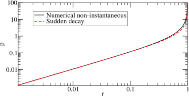
Figure 1: To achieve the same curvature perturbation transfer efficiency $r$ one needs to start from slightly different initial value of $p$ in the sudden-decay case (red dashed line) than in the non-instantaneous decay case (black solid line).

As mentioned in the beginning of this section the relation between $r$ and $p$ in the sudden-decay approximation is non-trivial. In the non-instantaneous decay case $r(p)$ is easy to find numerically from (61). In the sudden-decay case we can only determine $r_{\rm SD}(p)$ from (38) if we know $\Omega_{{\chi},{\rm dec}}(p)$.

Fortunately, a short-cut to the same result is provided by the differential equation (66). Using (57) we find from (66)

$$\int\frac{dp}{p}=\int\frac{3dr_{\rm SD}}{3r_{\rm SD}-2r_{\rm SD}^{2}-r_{\rm SD}^{3}}\,,$$ (67)

and hence

$$p\propto r_{\rm SD}(r_{\rm SD}+3)^{-1/4}(1-r_{\rm SD})^{-3/4}\,.$$ (68)

The constant of proportionality is not uniquely determined by the sudden-decay approximation, and corresponds to the arbitrariness in the definition of the decay time $H_{\rm dec}\sim\Gamma$.

What we can do is to use the limiting form of the analytic approximation to the numerical solution (50) for small $p$ to provide an overall normalisation for the sudden-decay approximation. This yields

$$p=\frac{3^{1/4}r_{\rm SD}}{0.924(r_{\rm SD}+3)^{1/4}(1-r_{\rm SD})^{3/4}}\,.$$ (69)

The above equation thus determines the value of $p$ that corresponds to a given value of the linear transfer function, $r_{\rm SD}$, in the sudden-decay approximation, and hence $\Omega_{{\chi},{\rm dec}}$ from Eq. (38). In Fig. 1 we show $p$ as a function of $r_{\rm SD}$ in the sudden-decay approximation and compare this with the numerical non-instantaneous decay result for $p(r)$.

Our form for $r_{\rm SD}(p)$ is quite different from that adopted by Malik and Lyth in their recent work Malik and Lyth (2006). They used a much simpler, but less accurate, estimate for $r(p)$ in the sudden-decay approximation:

$$r_{\rm ML}=\frac{p}{1+p}\,.$$ (70)

Although $r_{\rm ML}\to 1$ as $p\to\infty$ it fails to reproduce the correct linear coefficient as for $p\to 0$. The apparent error in the sudden-decay approximation for $f_{\rm{NL}}$ reported by Malik and Lyth Malik and Lyth (2006) (see for instance Figure 9 in that paper) is primarily due to this inaccuracy in the $r_{\rm ML}(p)$.

In what follows we have chosen to do all our comparisons of the sudden-decay approximation and numerical non-instantaneous decay results at common values of $r$. In other words, we have presented our results as a function of $r$ instead of $p$. After taking into account this fundamental difference in thinking, the results of Malik and Lyth (2006) agree with ours.

Now we are ready for the final comparison of ${f_{\rm{NL}}}_{\rm SD}(r)$, derived in the sudden-decay approximation with, ${f_{\rm{NL}}}(r)$ calculated numerically allowing for non-instantaneous decay. Fig. 2 shows that if $f_{\rm{NL}}>60$ ($r<0.02$) or $f_{\rm{NL}}<-1.16$ ($r>0.95$), the sudden decay result differs from the non-instantaneous decay result by less than $1\%$. Hence, when constraining the curvaton model with the current observational constraints on $f_{\rm{NL}}$ there is no need for an exact numerical calculation; using the sudden-decay approximation is sufficient. However, in the future experiments are expected to bring down the upper bound on $|f_{\rm{NL}}|$, and then constraining the curvaton model does require the numerical calculation presented here (or in Valiviita (24/03/2006); Malik and Lyth (2006)).

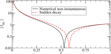
Figure 2: The non-linearity parameter $f_{\rm{NL}}$ as a function of curvature perturbation transfer efficiency $r=\zeta_{1}/\zeta_{{\chi}1}$. The analytical approximative, i.e., sudden-decay result (red dashed line) crosses zero at $r=0.58$ and is negative for $r>0.58$. The exact numerical result (black solid line) is negative for $r>0.53$. Here we assume that $g({\chi}_{\ast})$ is linear.

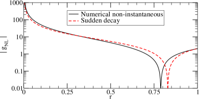
Figure 3: The non-linearity parameter $g_{\rm{NL}}$ as a function of curvature perturbation transfer efficiency $r=\zeta_{1}/\zeta_{{\chi}1}$. The analytical approximative, i.e., sudden-decay result (red dashed line) crosses zero at $r=0.83$ and is positive for $r>0.83$. The exact numerical result (black solid line) is positive for $r>0.79$. Here we assume that $g({\chi}_{\ast})$ is linear.

In Fig. 3 we compare $g_{\rm{NL}}$ in the sudden-decay approximation with the non-instantaneous decay result. The sudden-decay result for $g_{\rm{NL}}$ is much more inaccurate than for $f_{\rm{NL}}$. However, the present observational constraints on $g_{\rm{NL}}$ are so weak that again the sudden-decay approximation may be sufficient.

Let us end this subsection with a comment on numerical accuracy. Since the derivatives of $N(p)$ in (58) – (60) involve subtraction of nearly equal numbers, the calculation must be carried out carefully. The first requirement is that the integration step-size in $N$ is small enough compared to $\delta p$ that the two initial values $p_{i}$ and $p_{i+1}=p_{i}+\delta p$ really lead to numerically different values for $N_{i}=N(p_{i})$ and $N_{i+1}=N(p_{i+1})$. The accuracy of $N$ must be good enough to maintain enough significant figures in $\delta N=N_{i+1}-N_{i}$. The smaller the steps in $\delta p$ that we want to take the higher the accuracy in $N$ that we need. We calculate the first derivative at $p=p_{i}$ as an average of two nearby gradients

$$\left.{\frac{dN}{dp}}\right|_{p=p_{i}}=\frac{1}{2}\left(\frac{N_{i}-N_{i-1}}{p_{i}-p_{i-i}}+\frac{N_{i+1}-N_{i}}{p_{i+1}-p_{i}}\right)\,.$$ (71)

We use the same algorithm for the second derivative (with $N$ replaced by the result of the calculation of $dN/dp$) and for the third derivative (with $N$ replaced by the result of the calculation of $d^{2}N/dp^{2}$). As a result, the first derivative picks up contributions from 3 nearby points, the second derivative picks up weighted contributions from 5 nearby points and the third derivative from 7 nearby points. This procedure smooths out any residual numerical noise.

IV.3 An analytic approximation to the numerical result

The analytic approximation of $r(p)$, Eq. (50), with help of (57) gives

$$r^{\prime}\approx 2\times 1.24\left(1-r\right)\left[1-(1-r)^{\frac{1}{1.24}}\right]\frac{g^{\prime}}{g}\,.$$ (72)

Hence, from (64) we find an analytic approximation to the non-linearity parameter

$${f_{\rm{NL}}}_{\rm fit}=\frac{5}{4}\frac{1}{r}\left(1+\frac{gg^{\prime\prime}}{{g^{\prime}}^{2}}\right)$$ (73)

$$\quad+\frac{5}{4}\frac{1}{r^{2}}\left\{-2r+2\times 1.24\left(1-r\right)\left[1-(1-r)^{\frac{1}{1.24}}\right]\right\}\,.$$

The difference from the numerical result is non-negligible only when $f_{\rm{NL}}$ is extremely close to zero. Indeed, we find

$$\left|\frac{{f_{\rm{NL}}}_{\rm fit}-f_{\rm{NL}}}{f_{\rm{NL}}}\right|<1\%\,$$ (74)

if $r<0.501$ or $r>0.542$. The difference is larger than 5% only when $r\in[0.528,\,0.534]$.

V Probability density function

Thus far we have calculated the second- and third-order corrections to the curvature perturbation produced by the curvaton decay from which the leading order terms to the bispectrum and trispectrum can be calculated. However the $\delta N$-formalism allows us to describe the full non-linear probability density function on large scales for the non-linear primordial curvature perturbation defined in Eq. (2).

Assume we have two random variables $y$ and $z$, and the pdf of $y$ is $f(y)$. Furthermore, assume that the functional dependence of $z$ on $y$ is known, $z=z(y)$, and this mapping is a bijection. Then the probability of $z$ being in the interval $(z_{1},z_{2})$ is given by

$$P(z_{1}<z<z_{2})=\int_{z_{1}}^{z_{2}}\left|\frac{dy}{dz}\right|f(y)dz\,,$$ (75)

where the absolute value is needed in the case that $y(z)$ happens to be a decreasing function. Hence the pdf of the random variable $z$ is

$$\tilde{f}(z)=\left|\frac{dy(z)}{dz}\right|f[y(z)]\,.$$ (76)

In the multi-variable case the derivative would be replaced by the Jacobian determinant. For a Gaussian random variable, $y$, with mean $\mu_{y}$ and variance $\sigma_{y}^{2}$ we have

$$f(y)=\frac{1}{\sqrt{2\pi\sigma_{y}^{2}}}e^{-(y-\mu_{y})^{2}/(2\sigma_{y}^{2})}\,.$$ (77)

Since the first-order primordial curvature perturbation, $\zeta_{1}$, depends linearly on the initial Gaussian field perturbation, $\delta{\chi}_{\ast}$, we can take $\zeta_{1}$ as our Gaussian “reference” variable with mean $\mu_{\zeta_{1}}=0$ and variance

$$\sigma_{\zeta_{1}}=\frac{2}{3}r\frac{g^{\prime}}{g}\sigma_{\delta{\chi}_{*}}\,.$$ (78)

With this goal in our mind we have already written all our non-linear expressions for $\zeta$ as a function of $\zeta_{1}$. In the sudden-decay approximation we found an analytic functional dependence $\zeta=\zeta(\zeta_{1})$ and in the non-instantaneous decay case this function was found numerically. The mapping from $\zeta_{1}$ to $\zeta$ is not actually a bijection as there can be several values of $\zeta_{1}$ which are mapped onto the same value of $\zeta$. See Appendix A for the sudden-decay case. Calling these values ${\zeta_{1}}_{j}$, it is now easy to calculate the pdf of the non-linear primordial curvature perturbation

$$\tilde{f}(\zeta)=\sum_{j}\left|\frac{d\zeta_{1}}{d\zeta}\right|_{\zeta_{1}={\zeta_{1}}_{j}}\!\!\!f_{g}({\zeta_{1}}_{j})\,,$$ (79)

where $f_{g}(\zeta_{1})$ it the Gaussian pdf with $\mu=0$ and $\sigma=\sigma_{\zeta_{1}}$.

For simplicity we will assume in the rest of this section that there is no non-linear evolution of the curvaton field before it begins to oscillate, so that $g\propto{\chi}_{\ast}$, i.e., $g^{(n)}=0$ for $n\geq 2$. In principle one could also carry through the non-linear evolution of the curvaton field into the full numerical calculation of the pdf for the primordial curvature perturbation.

At the end of Appendix A we derive $\tilde{f}(\zeta)$ in the sudden-decay approximation, see Eq. (125). Here we continue by demonstrating the calculation of $\tilde{f}(\zeta)$ up to second order, which we will call $\tilde{f}_{2}(\zeta)$. From (4) we have $\zeta=\zeta_{1}+\frac{3}{5}f_{\rm{NL}}\zeta_{1}^{2}$ up to second order, i.e.,

$${\zeta_{1}}_{\pm}=\frac{5}{6f_{\rm{NL}}}\left(-1\pm\sqrt{1+12f_{\rm{NL}}\zeta/5}\right)\,.$$ (80)

Substituting this into (79) we find

$$\tilde{f}_{2}(\zeta)=\frac{1}{\sqrt{1+12f_{\rm{NL}}\zeta/5}}\frac{1}{\sqrt{2\pi\sigma_{\zeta_{1}}^{2}}}\\ \times\sum_{\pm}e^{-\left[\frac{5}{6f_{\rm{NL}}}\left(-1\pm\sqrt{1+12f_{\rm{NL}}\zeta/5}\right)\right]^{2}\Big{/}(2\sigma_{\zeta_{1}}^{2})}\,,$$ (81)

if $\zeta>-5/(12f_{\rm{NL}})$, and $\tilde{f}_{2}(\zeta)=0$ otherwise. If we want to evaluate $\tilde{f}_{2}(\zeta)$ for a particular value of the parameter $r$ we can substitute $f_{\rm{NL}}$ from (41) into (81) in the sudden-decay case, or use $f_{\rm{NL}}(r)$ as shown in Fig. 2 in the non-instantaneous decay case.

In Fig. 4(a) we compare the fully non-linear pdf $\tilde{f}(\zeta)$ (non-instantaneous decay) and $\tilde{f}_{\rm SD}(\zeta)$ (sudden decay) to the Gaussian $f_{g}(\zeta_{1})$ in the case when there is large non-Gaussianity ($r=0.00028$, $p=0.00030$, $f_{\rm{NL}}=4432$). In Fig. 5(a) we plot the pdfs in the case when $f_{\rm{NL}}$ has exactly the WMAP3 upper limit value ($r=0.010758$, $p=0.011560$, $f_{\rm{NL}}=114$). When the non-linearity parameter is very large, this kind of visual comparison reveals the non-Gaussianity, but already with $f_{\rm{NL}}=114$ the $\tilde{f}$ is virtually indistinguishable from the Gaussian $f_{g}$. However, in Fig. 4(b) and Fig. 5(b) we plot $\tilde{f}/f_{g}$ which reveals the non-Gaussianity even when $f_{\rm{NL}}=114$.

V.1 Moments of the distribution

The non-Gaussianity can be described quantitatively by calculating the moments of the pdf. Any pdf $f(z)$ should give a unit total probability

$$\int f(z)dz=1\,.$$ (82)

The mean can be calculated as

$$\mu_{z}=\int zf(z)dz\,.$$ (83)

and the $i^{\rm th}$ moment $m_{z}(i)$ is defined as

$$m_{z}(i)=\int(z-\mu)^{i}f(z)dz\,.$$ (84)

The second moment is the variance ($\sigma_{z}^{2}$), the third moment is called skewness, and the fourth moment kurtosis. As these moments can be extracted from the CMB maps it is enlightening to calculate the curvaton-model prediction for them.

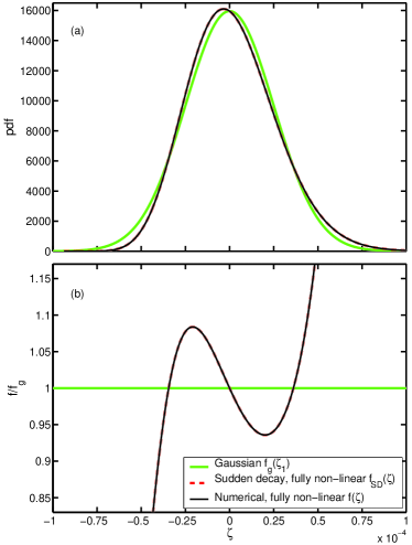
Figure 4: (a) Pdfs at $r=0.00028$ ($p=0.00030$, $f_{\rm{NL}}=4432$). Red dashed line is for the sudden decay, $\tilde{f}_{\rm SD}(\zeta)$, and black solid line for the non-instantaneous decay, $\tilde{f}(\zeta)$. The solid green/grey line is the Gaussian “reference”, $f_{g}(\zeta_{1})$. (b) The ratio of non-Gaussian pdfs to the Gaussian one.

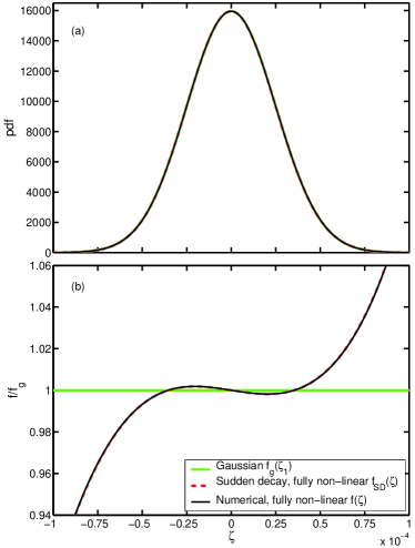
Figure 5: (a) Pdfs as in Fig. 4 but now at $r=0.010758$ ($p=0.011560$, $f_{\rm{NL}}=114$). In this figure the Gaussian reference (solid green/grey line) is completely indistinguishable from the fully non-linear (“non-Gaussian”) pdfs. (b) The ratio of non-Gaussian pdfs to the Gaussian one.

For Gaussian pdfs any odd moment (with $i\geq 3$) is zero, since the probability density is symmetric around the mean. The even moments of a Gaussian distribution are easy to calculate employing partial integration to give $m(4)=3\sigma^{4}$, $m(6)=15\sigma^{6}$, $m(8)=105\sigma^{8}$, $m(10)=945\sigma^{10}$, $m(12)=10395\sigma^{12}$, etc. Any departure from these values indicates that the pdf is non-Gaussian. If odd moments differ from zero, there is an asymmetric deviation from Gaussianity. If even moments are smaller than in the Gaussian case, the pdf is more sharply peaked than the Gaussian. If even moments are larger, the pdf is wider. The set of moments $\{\mu,m(i)|i=2...\infty\}$ encodes the same information of non-Gaussianity as our fully non-linear $\zeta(\zeta_{1})$ (or the expansion $\zeta=\sum_{n=1}^{\infty}\zeta_{n}/n!$). However, it should be noted that giving the value, for example, for $m_{\zeta}(3)$ is not simply equivalent to giving the value for $f_{\rm{NL}}$, because the moment picks up contributions from the fully non-linear $\zeta$, not just from $\zeta_{1}+\frac{3}{5}f_{\rm{NL}}\zeta_{1}^{2}$.

It turns out that the moments can be calculated very accurately using the $\delta N$-formalism, even in the non-instantaneous decay case, since we need not to calculate the derivatives of the local expansion, $N$, as was done in calculating $f_{\rm{NL}}$ or $g_{\rm{NL}}$. At first it seems that we would need $\tilde{f}(\zeta)$, which includes a numerical derivative $d\zeta_{1}/d\zeta$:

$$m_{\zeta}(i)=\int(\zeta-\mu)^{i}\tilde{f}(\zeta)d\zeta\,,$$ (85)

but substituting $\tilde{f}$ from Eq. (79) we end up with

$$m_{\zeta}(i)=\sum_{j}\int(\zeta-\mu)^{i}f_{g}(\zeta_{1j})d\zeta_{1j}\,.$$ (86)

Here the only numerically calculated quantity is $\zeta$ (and $\mu$).

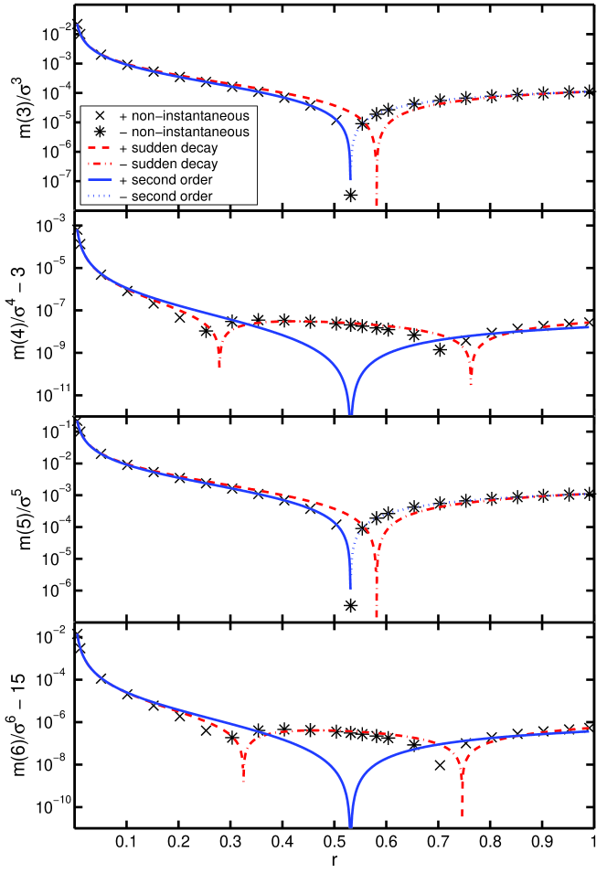
Figure 6: Third, fourth, fifth and sixth (from top to bottom) moments of the probability density function of the primordial curvature perturbation $\zeta$ as a function of the linear transfer parameter, $r$. The predictions using the fully non-linear sudden-decay approximation are shown by the dashed red line (dot-dashed for negative values), and the second-order results are shown by the solid blue line (dotted for negative values). The fully non-linear numerical results are indicated by black crosses (stars for negative values).

Calculating the moments in the second order expansion and comparing to the results of fully non-linear calculation (86) we can address the question whether $\sum_{n=3}^{\infty}\zeta_{n}/n!$ gives an important contribution to $\zeta$ and hence to the non-Gaussianity or whether the second order expansion $\zeta\approx\sum_{n=1}^{2}\zeta_{n}/n!$ is indeed accurate enough. To this end let us calculate in the second-order expansion the mean

$$\mu_{2} = \int\zeta f_{g}(\zeta_{1})d\zeta_{1}=\int\left(\zeta_{1}+\frac{3}{5}f_{\rm{NL}}\zeta_{1}^{2}\right)f_{g}(\zeta_{1})d\zeta_{1}$$ (87)

$$= \frac{3}{5}f_{\rm{NL}}\sigma^{2}_{\zeta_{1}}\,,$$

the variance

$$\sigma_{2}^{2} = \int\left(\zeta_{1}+\frac{3}{5}f_{\rm{NL}}\zeta_{1}^{2}-\frac{3}{5}f_{\rm{NL}}\sigma^{2}_{\zeta_{1}}\right)^{2}f_{g}(\zeta_{1})d\zeta_{1}$$ (88)

$$= \sigma^{2}_{\zeta_{1}}+2\left(\frac{3}{5}f_{\rm{NL}}\right)^{2}\!\!\sigma^{4}_{\zeta_{1}}\,,$$

the skewness

$$m_{2}(3) = 6\left(\frac{3}{5}f_{\rm{NL}}\right)\sigma^{4}_{\zeta_{1}}+8\left(\frac{3}{5}f_{\rm{NL}}\right)^{3}\!\!\sigma^{6}_{\zeta_{1}}\,,$$ (89)

and the kurtosis

$$\!\!\!\!\!\!m_{2}(4)\! = \!3\sigma^{4}_{\zeta_{1}}\!+\!60\left(\frac{3}{5}f_{\rm{NL}}\right)^{2}\!\!\sigma^{6}_{\zeta_{1}}\!+\!60\left(\frac{3}{5}f_{\rm{NL}}\right)^{4}\!\!\sigma^{8}_{\zeta_{1}}\!.$$ (90)

For higher moments in the second-order expansion we find

$$m_{2}(5) = 60\left(\frac{3}{5}f_{\rm{NL}}\right)\sigma^{6}_{\zeta_{1}}+680\left(\frac{3}{5}f_{\rm{NL}}\right)^{3}\sigma^{8}_{\zeta_{1}}$$ (91)

$$+ 544\left(\frac{3}{5}f_{\rm{NL}}\right)^{5}\sigma^{10}_{\zeta_{1}}\,,$$

and

$$m_{2}(6) = 15\sigma^{6}_{\zeta_{1}}+1170\left(\frac{3}{5}f_{\rm{NL}}\right)^{2}\sigma^{8}_{\zeta_{1}}$$ (92)

$$+ \!\!9060\!\left(\frac{3}{5}f_{\rm{NL}}\right)^{4}\!\!\!\sigma^{10}_{\zeta_{1}}+6040\!\left(\frac{3}{5}f_{\rm{NL}}\right)^{6}\!\!\!\sigma^{12}_{\zeta_{1}}\,.$$

From Eqs. (89) and (91) we find the leading order prediction

$$\frac{m_{2}(5)/\sigma^{5}}{m_{2}(3)/\sigma^{3}}=10\,,$$ (93)

and from Eqs. (90) and (92) we expect

$$\frac{m_{2}(6)/\sigma^{6}-15}{m_{2}(4)/\sigma^{4}-3}\approx\frac{1170}{60}=19.5\,,$$ (94)

at least when $f_{\rm{NL}}$ is small.

In Fig. 6 we plot the moments from the third up to the sixth one as a function of $r$. (For each value of $r$, it takes couple of hours to calculate the moments in the non-instantaneous decay case with our code on a typical PC. This comes about because we want to find $N$ with a relative error of less than $10^{-20}$ in order to have a sufficiently accurate result near to the peak of the pdf where $\zeta=\delta N$ is extremely close to zero. We need about $2\times 10^{5}$ steps integrating $N$ from the Friedmann equation, and we calculate $\zeta$ for $6001$ equally spaced values of $\zeta_{1}$ in the range $[-6\times 10^{-3},\,6\times 10^{-3}]$. Thus to produce a pdf for a fixed value of $r$ we need $10^{9}$ integration steps.) We compare the fully non-linear non-instantaneous decay result to the second-order results and to the fully non-linear sudden-decay result.

We find that results obtained using the fully non-linear sudden-decay approximation agree well with those obtained from the full non-instantaneous decay. The sudden-decay approximation accurately predicts the moments of the distribution for small values of $r$ where the non-Gaussianity is largest, and only fails to give the precise values of $r$ where the moments cross zero, very similar to what was seen previously when evaluating the non-linear parameters $f_{\rm{NL}}$ and $g_{\rm{NL}}$ in Sec. IV.

The expressions for the moments, given in Eqs. (87–92), calculated using only terms up to second-order in perturbation theory [but using the full numerical value for $f_{\rm{NL}}(r)$] are an excellent description of the odd moments of the distribution for all $r$. For even moments, the second-order expressions give the correct order magnitude, but cannot always reproduce the correct sign of the moments for $r>0.1$. In particular we see that the even moments of the distribution predicted at second-order are always larger than the Gaussian value (setting $f_{\rm{NL}}=0$), whereas the full numerical results show that the even moments can be less than the Gaussian value. To describe the deviations from Gaussianity in the even moments we need to include third-order terms. For example the variance, to third order, is given by

$$\sigma_{3}^{2} = \textstyle\sigma^{2}_{\zeta_{1}}+\left[2\left(\frac{3}{5}f_{\rm{NL}}\right)^{2}+6\left(\frac{9}{25}g_{\rm{NL}}\right)\right]\sigma^{4}_{\zeta_{1}}$$ (95)

$$+ \textstyle 15\left(\frac{9}{25}g_{\rm{NL}}\right)^{2}\sigma^{6}_{\zeta_{1}}\,,$$

where the expression in square brackets gives the leading order correction to the Gaussian result. This correction can be negative due to negative $g_{\rm{NL}}$ when $f_{\rm{NL}}$ is small. On the contrary, the skewness up to third order is

$$m_{3}(3)=\textstyle 6\left(\frac{3}{5}f_{\rm{NL}}\right)\sigma^{4}_{\zeta_{1}}+\Big{[}8\left(\frac{3}{5}f_{\rm{NL}}\right)^{3}+72\left(\frac{3}{5}f_{\rm{NL}}\right)\\ \times\textstyle\left(\frac{9}{25}g_{\rm{NL}}\right)\Big{]}\sigma^{6}_{\zeta_{1}}+270\left(\frac{3}{5}f_{\rm{NL}}\right)\left(\frac{9}{25}g_{\rm{NL}}\right)^{2}\sigma^{8}_{\zeta_{1}}\,,$$ (96)

where the first term is the leading order correction to the Gaussian result [$m(3)=0$]. As seen this correction does not have $g_{\rm{NL}}$ term so that already the second order expansion leads to approximately correct results.

Although not shown in the Fig. 6 we have verified that the third-order perturbation theory (using the numerical results for $f_{\rm{NL}}$ and $g_{\rm{NL}}$) accurately reproduce all the moments of the distribution as a function of $r$ at least up to and including the sixth moment.

The results (see Fig. 6) obey the predictions of Eqs. (93) and (94). In particular, the fully non-linear numerical calculation also reproduces the predicted ratios of the moments.

VI Variance on small scales

We now consider the effect of a (possibly) large contribution to the curvaton density from smaller scale modes, compared with the cosmological scales probed directly, for instance, by the CMB anisotropies. This situation was recently discussed by Linde and Mukhanov Linde and Mukhanov (2006) (see also Linde and Mukhanov (1997); Lyth (2006)). Such smaller scale modes might contribute significantly to the average curvaton energy density on larger scales if the curvaton field power spectrum rises on smaller scales, or if some of the fraction (even if it is a small fraction) of the energy from the inflaton decay at the end of inflation is transfered to the curvaton Linde and Mukhanov (2006). In either case we will describe this by a small scale variance in the curvaton field up to some averaging scale

$$\Delta_{s}^{2}=\frac{\langle\delta{\chi}^{2}\rangle_{s}}{\bar{\chi}^{2}}\,.$$ (97)

The key observation is that these small-scale field fluctuations on spatially-flat hypersurfaces are uncorrelated with the field perturbations on larger scales. Thus there is an additional contribution to the average curvaton energy density

$$\bar{\rho}_{\chi}=\frac{1}{2}m^{2}(1+\Delta_{s}^{2})\bar{\chi}^{2}\,,$$ (98)

which is homogeneous on large scales. In effect the curvaton density can be spilt into two parts: one that is perturbed on large scales, and one that is not.

We can include the contribution from this small-scale variance in our non-linear expression (34) for the curvature perturbation, $\zeta$, in the sudden-decay approximation where the curvaton decays on a uniform-density hypersurface, to give the equation

$$(1-\Omega_{{\chi},{\rm{dec}}})e^{-4\zeta} + \frac{1}{1+\Delta_{s}^{2}}\Omega_{{\chi},{\rm{dec}}}e^{3(\zeta_{\chi}-\zeta)}$$ (99)

$$+ \frac{\Delta_{s}^{2}}{1+\Delta_{s}^{2}}\Omega_{{\chi},{\rm{dec}}}e^{-3\zeta}=1\,,$$

where we have set to zero any pre-existing perturbation in the radiation, $\zeta_{r}=0$.

At first order this shows how the resulting curvature perturbation on large scales is suppressed by the small-scale variance:

$$\zeta_{1}=\frac{r}{1+\Delta_{s}^{2}}\zeta_{{\chi}1}\,,$$ (100)

where $r$ is given by Eq. (38) in the sudden-decay approximation, and we use $\zeta_{{\chi}1}$ to denote the fractional field perturbation on large scales, given in Eq. (23).

However small-scale variance also affects the non-Gaussianity at second- and higher-orders. At second-order we find

$$\zeta_{2}=\left[\frac{3(1+\Delta_{s}^{2})}{2r}\left(1+\frac{gg^{\prime\prime}}{g^{\prime 2}}\right)-2-r\right]\zeta_{1}^{2}\,,$$ (101)

and thus we have

$$f_{\rm{NL}}=(1+\Delta_{s}^{2})\frac{5}{4r}\left(1+\frac{gg^{\prime\prime}}{g^{\prime 2}}\right)-\frac{5}{3}-\frac{5r}{6}\,.$$ (102)

Note that the small-scale variance, although homogeneous, is not equivalent to additional homogeneous radiation due to its non-relativistic equation of state.

If we allow for non-instantaneous curvaton decay we find

$$f_{\rm{NL}}=(1+\Delta_{s}^{2})\frac{5}{4r}\left(1+\frac{gg^{\prime\prime}}{g^{\prime 2}}\right)+\frac{5}{6}\frac{d^{2}N/dp^{2}}{\left(dN/dp\right)^{2}}\,,$$ (103)

where any $\Delta_{s}^{2}$ dependence in the second term on the right-hand-side cancels out so that we can use the numerical results presented in Sec. IV to evaluate this term.

VI.1 Observational constraints on small-scale variance

The fact that the non-linearity parameter grows with the small-scale variance means that we can constrain the small-scale variance from constraints on the non-linearity parameter $f_{\rm{NL}}$ on larger scales.

In practice the non-linearity at each successive order still depends on the non-linear evolution function for the curvaton field, $g({\chi}_{*})$. Hence we cannot rule out models where the small-scale variance is large, but its effect is precisely cancelled by the non-linear evolution. For simplicity we assume in the following that the non-linear evolution is negligible so that $g^{\prime\prime}$ and higher derivatives can be set to zero.

Recalling, that $r\leq 1$ and $-54<f_{\rm{NL}}<114$ (from WMAP3 Spergel et al. (2006)) we find an upper bound

$$\Delta_{s}^{2}<90\,.$$ (104)

VI.2 Observational constraints on variance on CMB scales

On the scales directly probed by CMB observations, the constraint on the variance will be much tighter, since in addition to $f_{\rm{NL}}$ constraint we observe

$$\langle\zeta_{1}^{2}\rangle_{\rm CMB}=A^{2}\,,$$ (105)

with $A^{2}\simeq 6.25\times 10^{-10}$. Substituting (100) with (23) into the left hand side we get

$$\frac{4}{9}\frac{\Delta_{\rm CMB}^{2}}{(1+\Delta_{s}^{2})^{2}}r^{2}=A^{2}\,,$$ (106)

where

$$\Delta_{\rm CMB}^{2}=\frac{\langle\delta{\chi}^{2}\rangle_{\rm CMB}}{\bar{\chi}^{2}}\,.$$ (107)

Equation (106) gives

$$\Delta^{2}_{\rm CMB}=\frac{9}{4}A^{2}\frac{(1+\Delta_{s}^{2})^{2}}{r^{2}}\,,$$ (108)

and eliminating $(1+\Delta_{s}^{2})^{2}/r^{2}$ with help of (103) we end up with

$$\Delta^{2}_{\rm CMB}=\frac{9}{4}A^{2}\left(\frac{4}{5}f_{\rm{NL}}-\frac{2}{3}\frac{d^{2}N/dp^{2}}{\left(dN/dp\right)^{2}}\right)^{2}\,.$$ (109)

The maximum of the absolute value of the second term in the parenthesis is numerically found to be always less than $2$. Thus, employing the triangle inequality, we find

$$\Delta^{2}_{\rm CMB}<\frac{9}{4}A^{2}\left(|\frac{4}{5}f_{\rm{NL}}|+2\right)^{2}\,.$$ (110)

But the WMAP3 upper limit for $|\frac{4}{5}f_{\rm{NL}}|$ is $91$, which implies

$$\Delta^{2}_{\rm CMB}<\frac{9}{4}A^{2}\times 93^{2}=1.2\times 10^{-5}\,.$$ (111)

VII Conclusions

In this paper we have presented for the first time the fully non-linear probability density function (pdf) for the primordial curvature perturbation on large scales in the curvaton scenario using the $\delta N$-formalism. By solving the non-linear evolution equations in an unperturbed (FRW) universe one can construct the local expansion upto a final uniform density as a function of the initial curvaton field value, $N({\chi})$. Assuming a Gaussian form for the initial field distribution on large scales (as would be expected for a weakly coupled scalar field after inflation) it is straightforward to construct the probability density function for $\delta N$ and hence the non-linear curvature perturbation $\zeta$, defined in Eq. (2). This procedure is particularly simple in the case where the local expansion is a function of a single scalar field, such as the curvaton, but it is also straightforward to apply to multiple fields whose initial distributions on large scales are known.

In the sudden-decay approximation where it is assumed that the curvaton decays instantaneously, when $H\sim\Gamma$, we have presented a simple non-linear analytic expression, Eq. (34), relating the primordial curvature perturbation to the initial curvaton perturbation. We have compared analytic results in the sudden-decay approximation, with our results derived from direct numerical integration of the full coupled equations for the local radiation and curvaton energy densities and found good quantitative agreement.

In particular we have calculated the leading-order contributions to the primordial bispectrum and trispectrum, including for the first time the effect of third-order terms in the curvature perturbation. In some cases Lyth (2004); Enqvist and Nurmi (2005) non-linear evolution of the curvaton field on super-Hubble scales, after Hubble-exit during inflation, but before the curvaton begins to oscillate about the minimum of its potential, could lead to a suppression of the leading order contribution to the primordial bispectrum. We have shown that in this case there will instead be a large contribution to the primordial trispectrum, unless there is an additional cancellation in the third-order term.

We have computed numerically the moments of the pdf for the primordial curvature perturbation up to and including the sixth-order moment for a range of values of the linear transfer coefficient, $r$. To accurately reproduce the even moments of the distribution we need to go beyond the second-order terms in the curvature perturbation (described by the non-linearity parameter $f_{\rm{NL}}$) and include higher-order terms.

One example of how non-Gaussianity can be used to constrain model parameters is the case when the curvaton field has a large variance on small scales, as recently proposed by Linde and Mukhanov Linde and Mukhanov (2006). In this case the suppression of the linear curvature perturbation is accompanied by an increase in non-Gaussianity. We have shown that in this case limits on the primordial bispectrum can be used to place limits on the small scale variance.

The calculations presented here should enable the curvaton model to be subjected to a range of tests of non-Gaussianity, going beyond just the bispectrum. In the simplest models (neglecting non-linear evolution of the field before it decays) the non-Gaussianity is a function of a single parameter, $r$, which is the linear transfer coefficient relating the first-order primordial curvature perturbation with the curvaton perturbation at Hubble-exit during inflation. Multiple tests of the form of any primordial non-Gaussianity could offer consistency tests of the curvaton scenario.

Appendix A

In this appendix we solve the primordial curvature perturbation $\zeta$ as a function of initial Gaussian field perturbation $\delta_{1}{\chi}$ in the sudden-decay approximation. We also solve the inverse problem, i.e., find $\delta_{1}{\chi}/\bar{\chi}$ (or $\zeta_{1}$) as a function of $\zeta$. Using these results we derive an analytic expression for the (non-Gaussian) probability density function of $\zeta$; $\tilde{f}(\zeta)$.

We can rewrite Eq. (35) in the form

$$e^{4\zeta}-\left[\frac{4r}{3+r}e^{3\zeta_{\chi}}\right]e^{\zeta}+\left[\frac{3r-3}{3+r}\right]=0\,,$$ (112)

where $r=3\Omega_{{\chi},{\rm{dec}}}/(4-\Omega_{{\chi},{\rm{dec}}})$. This is a fourth degree equation for $X=e^{\zeta}$. The solution of this full non-linear equation which gives the primordial curvature perturbation as a function of initial Gaussian curvaton field ${\chi}_{\ast}({\bf x})$ is

$$\zeta=\ln(X)\,,$$ (113)

with

$$X=K^{1/2}\frac{1+\sqrt{ArK^{-3/2}-1}}{(3+r)^{1/3}}\,,$$ (114)

where

$$A \stackrel{{\scriptstyle\mbox{\tiny{def}}}}{{=}} e^{3\zeta_{\chi}}=\frac{\rho_{{\chi},\rm osc}({\bf x})}{\bar{\rho}_{{\chi},\rm osc}}=\left[\frac{g({\chi}_{\ast}({\bf x}))}{g(\bar{\chi}_{\ast})}\right]^{2}\,,$$ (115)

$$K \stackrel{{\scriptstyle\mbox{\tiny{def}}}}{{=}} \textstyle{\frac{1}{2}}\left[P^{1/3}+(r-1)(3+r)^{1/3}P^{-1/3}\right]\,,$$ (116)

$$P \stackrel{{\scriptstyle\mbox{\tiny{def}}}}{{=}} (Ar)^{2}+\left[(Ar)^{4}-(3+r)(r-1)^{3}\right]^{1/2}\,.$$ (117)

The inverse problem (solving initial ${\chi}/\bar{\chi}$ as a function of $\zeta$) is much simpler. Namely, Eq. (112) gives immediately

$$e^{3\zeta_{\chi}}=\frac{3+r}{4r}e^{3\zeta}+\frac{3r-3}{4r}e^{-\zeta}\,,$$ (118)

and here $e^{3\zeta_{\chi}}=g^{2}[{\chi}_{\ast}({\bf x})]/g^{2}(\bar{\chi}_{\ast})={\chi}^{2}({\bf x})/\bar{\chi}^{2}$.

Assuming that there is no non-linear evolution between the Hubble exit and start of curvaton oscillation [$g^{(n)}=0$ for $n>1$] the left hand side of (118) is exactly [see Eq. (19)]

$$e^{3\zeta_{\chi}}=\left(1+\frac{\delta_{1}{\chi}}{\bar{\chi}}\right)^{2}=1+2\frac{\delta_{1}{\chi}}{\bar{\chi}}+\left(\frac{\delta_{1}{\chi}}{\bar{\chi}}\right)^{2}\,.$$ (119)

Hence (118) simplifies to a second degree equation for $\delta_{1}{\chi}/\bar{\chi}$. The solutions are

$$\left(\frac{\delta_{1}{\chi}}{\bar{\chi}}\right)_{\pm}=-1\pm\left[\frac{3+r}{4r}e^{3\zeta}+\frac{3r-3}{4r}e^{-\zeta}\right]^{1/2}\,,$$ (120)

where the “$+$” sign corresponds to a small perturbation and “$-$” sign would give $|\delta_{1}{\chi}/\bar{\chi}|\sim 1$. An alternative Gaussian “reference variable” is the linear end result $\zeta_{1}$. From (37) and (23) we have $\zeta_{1}=\frac{2}{3}r\frac{\delta_{1}{\chi}}{\bar{\chi}}$. In Sec. V we will need a derivative of this Gaussian random variable $\zeta_{1}$ with respect to $\zeta$. Using (120) we easily find

$$\frac{d\zeta_{1\pm}}{d\zeta} = \pm\frac{1}{3}r\left[3\frac{3+r}{4r}e^{3\zeta}-\frac{3r-3}{4r}e^{-\zeta}\right]$$ (121)

$$\ \ \ \ \times\left[\frac{3+r}{4r}e^{3\zeta}+\frac{3r-3}{4r}e^{-\zeta}\right]^{-1/2}\!\!\!\!\!\!\!.$$

Hence the full non-Gaussian probability density function for $\zeta$ is

$$\tilde{f}(\zeta)=\tilde{f}_{-}(\zeta)+\tilde{f}_{+}(\zeta)\,,$$ (122)

where

$$\tilde{f}_{\pm}(\zeta) = \left|\frac{d\zeta_{1\pm}}{d\zeta}\right|f_{g}(\zeta_{1\pm})\,,$$ (123)

and

$$f_{g}(\zeta_{1\pm})=\frac{1}{\sqrt{2\pi\sigma_{g}^{2}}}e^{-\zeta_{1\pm}^{2}/(2\sigma_{g}^{2})}$$ (124)

with $\zeta_{1\pm}$ being $2r/3$ times the rhs of Eq. (120). Here $f_{g}(\zeta_{1})$ is the Gaussian pdf for the first order perturbation $\zeta_{1}$ with variance $\sigma_{g}^{2}=\sigma_{\zeta_{1}}^{2}$ ($\sim 6.25\times 10^{-10}$ to match the observations), and mean $\mu=0$. In practice, $\tilde{f}_{-}(\zeta)$ could be neglected, because $f_{g}(\zeta_{1-})$ is typically of the order $\exp(-10^{10})$. Substituting all ingredients into (122) the pdf reads

$$\tilde{f}_{\rm SD}(\zeta) = \frac{1}{\sqrt{2\pi\sigma_{g}^{2}}}\frac{1}{2}\Big{[}(3+r)e^{3\zeta}+(1-r)e^{-\zeta}\Big{]}\left[\frac{3+r}{r}e^{3\zeta}+\frac{3r-3}{r}e^{-\zeta}\right]^{-1/2}$$ (125)

$$\times \sum_{\pm}\exp\left\{-\frac{4}{9}r^{2}\left[-1\pm\left(\frac{3+r}{4r}e^{3\zeta}+\frac{3r-3}{4r}e^{-\zeta}\right)^{1/2}\right]^{2}\Big{/}(2\sigma_{g}^{2})\right\}\,,$$

where the subscript SD reminds us that this is the sudden-decay result.

References

- Komatsu and Spergel (2001) E. Komatsu and D. N. Spergel, Phys. Rev. D63, 063002 (2001), eprint astro-ph/0005036.
- Maldacena (2003) J. M. Maldacena, JHEP 05, 013 (2003), eprint astro-ph/0210603.
- Spergel et al. (2006) D. N. Spergel et al. (2006), eprint astro-ph/0603449.
- Lyth and Wands (2002) D. H. Lyth and D. Wands, Phys. Lett. B524, 5 (2002), eprint hep-ph/0110002.
- Enqvist and Sloth (2002) K. Enqvist and M. S. Sloth, Nucl. Phys. B626, 395 (2002), eprint hep-ph/0109214.
- Moroi and Takahashi (2001) T. Moroi and T. Takahashi, Phys. Lett. B522, 215 (2001), eprint hep-ph/0110096.
- Enqvist et al. (2003) K. Enqvist, S. Kasuya, and A. Mazumdar, Phys. Rev. Lett. 90, 091302 (2003), eprint hep-ph/0211147.
- Allahverdi et al. (2006) R. Allahverdi, K. Enqvist, A. Jokinen, and A. Mazumdar (2006), eprint hep-ph/0603255.
- Bartolo and Liddle (2002) N. Bartolo and A. R. Liddle, Phys. Rev. D65, 121301 (2002), eprint astro-ph/0203076.
- Enqvist et al. (2000) K. Enqvist, H. Kurki-Suonio, and J. Valiviita, Phys. Rev. D62, 103003 (2000), eprint astro-ph/0006429.
- Enqvist et al. (2002) K. Enqvist, H. Kurki-Suonio, and J. Valiviita, Phys. Rev. D65, 043002 (2002), eprint astro-ph/0108422.
- Lyth et al. (2003) D. H. Lyth, C. Ungarelli, and D. Wands, Phys. Rev. D67, 023503 (2003), eprint astro-ph/0208055.
- Trotta (2006) R. Trotta (2006), eprint astro-ph/0608116.
- Lewis (2006) A. Lewis (2006), eprint astro-ph/0603753.
- Bean et al. (2006) R. Bean, J. Dunkley, and E. Pierpaoli, Phys. Rev. D74, 063503 (2006), eprint astro-ph/0606685.
- Sasaki and Tanaka (1998) M. Sasaki and T. Tanaka, Prog. Theor. Phys. 99, 763 (1998), eprint gr-qc/9801017.
- Wands et al. (2000) D. Wands, K. A. Malik, D. H. Lyth, and A. R. Liddle, Phys. Rev. D62, 043527 (2000), eprint astro-ph/0003278.
- Starobinsky (1985) A. A. Starobinsky, JETP Lett. 42, 152 (1985).
- Sasaki and Stewart (1996) M. Sasaki and E. D. Stewart, Prog. Theor. Phys. 95, 71 (1996), eprint astro-ph/9507001.
- Lyth and Rodriguez (2005) D. H. Lyth and Y. Rodriguez, Phys. Rev. Lett. 95, 121302 (2005), eprint astro-ph/0504045.
- Lyth et al. (2005) D. H. Lyth, K. A. Malik, and M. Sasaki, JCAP 0505, 004 (2005), eprint astro-ph/0411220.
- Okamoto and Hu (2002) T. Okamoto and W. Hu, Phys. Rev. D66, 063008 (2002), eprint astro-ph/0206155.
- Kogo and Komatsu (2006) N. Kogo and E. Komatsu, Phys. Rev. D73, 083007 (2006), eprint astro-ph/0602099.
- Lyth and Wands (2003) D. H. Lyth and D. Wands, Phys. Rev. D68, 103515 (2003), eprint astro-ph/0306498.
- Rigopoulos and Shellard (2003) G. I. Rigopoulos and E. P. S. Shellard, Phys. Rev. D68, 123518 (2003), eprint astro-ph/0306620.
- Malik and Wands (2004) K. A. Malik and D. Wands, Class. Quant. Grav. 21, L65 (2004), eprint astro-ph/0307055.
- Langlois and Vernizzi (2005) D. Langlois and F. Vernizzi, Phys. Rev. D72, 103501 (2005), eprint astro-ph/0509078.
- Boubekeur and Lyth (2006) L. Boubekeur and D. H. Lyth, Phys. Rev. D73, 021301 (2006), eprint astro-ph/0504046.
- Bartolo et al. (2004) N. Bartolo, S. Matarrese, and A. Riotto, Phys. Rev. Lett. 93, 231301 (2004), eprint astro-ph/0407505.
- Linde and Mukhanov (1997) A. D. Linde and V. F. Mukhanov, Phys. Rev. D56, 535 (1997), eprint astro-ph/9610219.
- Linde and Mukhanov (2006) A. Linde and V. Mukhanov, JCAP 0604, 009 (2006), eprint astro-ph/0511736.
- Seery and Lidsey (2005) D. Seery and J. E. Lidsey, JCAP 0509, 011 (2005), eprint astro-ph/0506056.
- Lyth and Zaballa (2005) D. H. Lyth and I. Zaballa, JCAP 0510, 005 (2005), eprint astro-ph/0507608.
- Seery et al. (2006) D. Seery, J. E. Lidsey, and M. S. Sloth (2006), eprint astro-ph/0610210.
- Lyth (2004) D. H. Lyth, Phys. Lett. B579, 239 (2004), eprint hep-th/0308110.
- Enqvist and Nurmi (2005) K. Enqvist and S. Nurmi, JCAP 0510, 013 (2005), eprint astro-ph/0508573.
- Malik et al. (2003) K. A. Malik, D. Wands, and C. Ungarelli, Phys. Rev. D67, 063516 (2003), eprint astro-ph/0211602.
- Gupta et al. (2004) S. Gupta, K. A. Malik, and D. Wands, Phys. Rev. D69, 063513 (2004), eprint astro-ph/0311562.
- Malik (2005) K. A. Malik, JCAP 0511, 005 (2005), eprint astro-ph/0506532.
- Malik and Lyth (2006) K. A. Malik and D. H. Lyth, JCAP 0609, 008 (2006), eprint astro-ph/0604387.
- Press et al. (1992) W. H. Press, S. A. Teukolsky, W. T. Vetterling, and B. P. Flannery, Numerical recipes in FORTRAN. The art of scientific computing (Cambridge: University Press, —c1992, 2nd ed., 1992).
- Valiviita (24/03/2006) J. Valiviita (24/03/2006), talk in 40th Rencontres de Moriond: Contents and Structures of the Universe, La Thuile, Italy. J. Valiviita, M. Sasaki and D. Wands, submitted to appear in the 40th Rencontres de Moriond proceedings, eprint astro-ph/0610001.
- Lyth (2006) D. H. Lyth, JCAP 0606, 015 (2006), eprint astro-ph/0602285.
- Ferrer et al. (2004) F. Ferrer, S. Rasanen, and J. Valiviita, JCAP 0410, 010 (2004), eprint astro-ph/0407300.
- Kurki-Suonio et al. (2005) H. Kurki-Suonio, V. Muhonen, and J. Valiviita, Phys. Rev. D71, 063005 (2005), eprint astro-ph/0412439.