A universal decline law of classical novae

Abstract

We calculate many different nova light curves for a variety of white dwarf masses and chemical compositions, with the assumption that free-free emission from optically thin ejecta dominates the continuum flux. We show that all these light curves are homologous and a universal law can be derived by introducing a “time scaling factor.” The template light curve for the universal law has a slope of the flux, $F\propto t^{-1.75}$, in the middle part (from $\sim 2$ to $\sim 6$ mag below the optical maximum) but it declines more steeply, $F\propto t^{-3.5}$, in the later part (from $\sim 6$ to $\sim 10$ mag), where $t$ is the time from the outburst in units of days. This break on the light curve is due to a quick decrease in the wind mass loss rate. The nova evolutions are approximately scaled by the time of break. Once the time of break is observationally determined, we can derive the period of a UV burst phase, the duration of optically thick wind phase, and the turnoff date of hydrogen shell-burning. An empirical observational formula, $t_{3}=(1.68\pm 0.08)~{}t_{2}+(1.9\pm 1.5){\rm~{}days}$, is derived from the relation of $F\propto t^{-1.75}$, where $t_{2}$ and $t_{3}$ are the times in days during which a nova decays by 2 and 3 mag from the optical maximum, respectively. We have applied our template light curve model to the three well-observed novae, V1500 Cyg (catalog ), V1668 Cyg (catalog ), and V1974 Cyg (catalog ). Our theoretical light curves show excellent agreement with the optical $y$ and infrared $J$, $H$, $K$ light curves. The continuum UV 1455 Å light curves observed with IUE are well reproduced. The turn-on and turn-off of supersoft X-ray observed with ROSAT are also explained simultaneously by our model. The WD mass is estimated, from the light curve fitting, to be $M_{\rm WD}\approx 1.15~{}M_{\sun}$ for V1500 Cyg (catalog ), $M_{\rm WD}\approx 0.95~{}M_{\sun}$ for V1668 Cyg (catalog ), and $M_{\rm WD}\approx 0.95-1.05~{}M_{\sun}$ for V1974 Cyg (catalog ), together with the appropriate chemical compositions of the ejecta.

1. Introduction

It has been widely accepted that a classical nova is a result of thermonuclear runaway on a mass-accreting white dwarf (WD) in a close binary system (e.g., Warner, 1995, for a review). Theoretical studies have elucidated full cycles of nova outbursts, i.e., from the mass accretion stage to the end of a nova outburst (e.g., Prialnik & Kovetz, 1995) and developments of light curves for various speed classes of novae (e.g., Kato & Hachisu, 1994; Kato, 1994, 1997). However, detailed studies of individual objects such as light curve analysis have not been fully done yet except for the recurrent novae (e.g., Hachisu & Kato, 2000a, b, 2001a, 2001b, 2003a, 2006a; Hachisu et al., 2000, 2003). In order to further develop a quantitative study of nova light curves, a new approach is required, from which we can derive the WD mass, ejecta mass, and duration of the nova outburst.

On the other hand, some characteristic features and common properties of nova light curves have been suggested, the reasons for which we do not yet fully understand. For example, infrared (IR) light curves of novae often show a decline law of $F_{\lambda}\propto t^{-\alpha}$, i.e., the flux at the wavelength $\lambda$ decays proportionally to a power of time from the outburst. Ennis et al. (1977) suggested that near IR $JHK$ fluxes of V1500 Cyg (catalog ) (Nova Cygni 1975 (catalog )) are proportional to $t^{-2}$ in the early stages of nova explosions, while at later times they decay more steeply as $t^{-3}$ (see also, Kawara et al., 1976; Gallagher & Ney, 1976). Woodward et al. (1997) found that near-infrared light curves of V1974 Cyg (catalog ) (Nova Cygni 1992 (catalog )) showed a power law of $\alpha\sim 1.5$ in the early 100 days.

Recently, Hachisu & Kato (2005) explained these power-law declines as free-free emission from an optically thin plasma outside the photosphere. Here we further extend their approach and develop a light curve model that is widely applicable to optical and IR light curves of various types of novae. Section 2 describes our basic idea and methods as well as our light curve models. We propose theoretical nova light curves having a universal decline law of $F_{\lambda}\propto t^{-\alpha}$, regardless of the WD mass, chemical composition of the envelope, or observational wavelength bands in optical and IR. Then we apply our method to three classical novae, i.e., V1500 Cyg (catalog ) in §3, V1668 Cyg (catalog ) (Nova Cygni 1978 (catalog )) in §4, and V1974 Cyg (catalog ) in §5. Discussion follows in §6, and finally we summarize our results in §7.

2. Modeling of nova light curves

After the thermonuclear runaway sets in on a mass-accreting WD, its envelope expands greatly to $R_{\rm ph}\gtrsim 100~{}R_{\sun}$ and a large part of the envelope is ejected as a wind. Figure 1 illustrates a typical nova evolution, from the maximum expansion of the photosphere to the end of hydrogen burning. At the very early expansion phase, the photosphere expands together with the ejecta. Then the photosphere lags behind the head of ejecta as its density decreases. Figure 2 depicts a schematic illustration of such a nova envelope, in which free-free emission from an optically thin plasma contributes to the optical and IR continuum fluxes. The photosphere eventually begins to shrink at or around the optical maximum. The nova envelope settles in a steady state after the optical maximum until the end of hydrogen shell burning (see Fig. 1).

2.1. Optically thick wind model

The decay phase of novae can be well represented with a sequence of steady-state solutions (e.g., Kato & Hachisu, 1994, and references therein). Using the same method and numerical techniques as in Kato & Hachisu (1994), we have calculated theoretical models of nova outbursts.

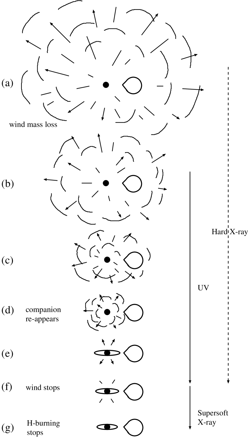
Figure 1.— Evolution of nova outbursts: $(a)$ after a nova explosion sets in, the photosphere expands greatly up to $\gtrsim 100~{}R_{\sun}$, and the companion star is engulfed deep inside the photosphere; $(b)$ after the maximum expansion, the photospheric radius shrinks with time and free-free emission dominates the flux at relatively longer wavelengths; $(c)$ a large part of the envelope matter is blown in the wind and the photosphere moves further inside; $(d)$ the companion eventually emerges from the WD photosphere and an accretion disk may appear or reestablished again; $(e)$ the photosphere further shrinks to a size of $\lesssim 0.1~{}R_{\sun}$; $(f)$ the optically thick wind stops; $(g)$ hydrogen nuclear burning stops and the nova enters a cooling phase. Hard X-rays may originate from internal shocks between ejecta (or a bow shock between ejecta and the companion) from stage $(a)$ to $(f)$ as indicated by a dashed line. The ultraviolet (UV) flux dominates from stage $(b)$ to $(f)$. Then the supersoft X-ray flux replaces the UV flux from stage $(f)$ to $(g)$.

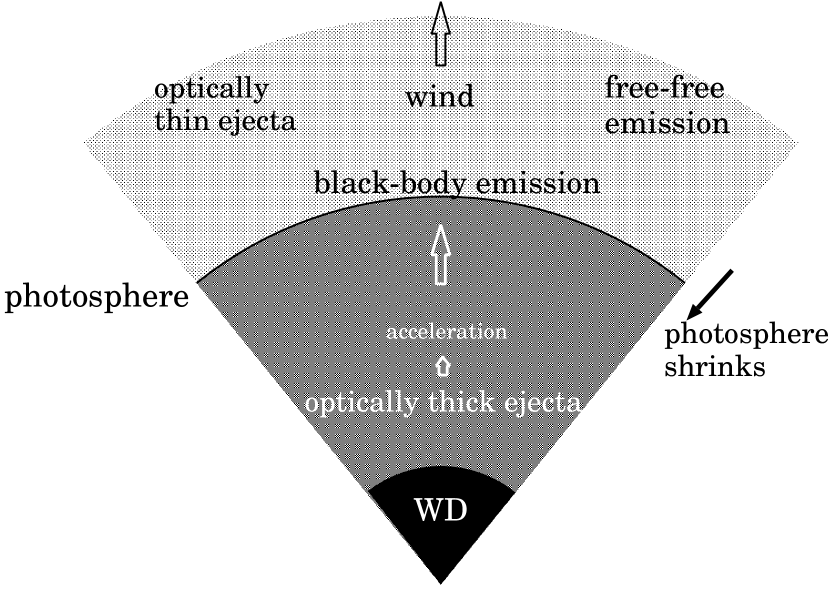
Figure 2.— A schematic configuration of our nova ejection model: A large part of the initial envelope mass is ejected by the winds, which are accelerated deep inside the photosphere. After the optical maximum, that is, after the maximum expansion of the photosphere, the photosphere begins to shrink whereas the ejecta are expanding. The optically thin layer emits free-free radiation at relatively longer wavelengths while blackbody radiation from the photosphere dominates at shorter wavelengths.

Table 1Chemical abundance of classical novae

object	H	CNO	Ne	Na-Fe	reference
V382 Vel (catalog ) 1999	0.47	0.0018	0.0099	0.0069	Augusto & Diaz (2003)
V382 Vel (catalog ) 1999	0.66	0.043	0.027	0.0030	Shore et al. (2003)
CP Cru (catalog ) 1996	0.47	0.18	0.047	0.0026	Lyke et al. (2003)
V723 Cas (catalog ) 1995	0.52	0.064	0.052	0.042	Iijima (2006)
V1425 Aql (catalog ) 1995	0.51	0.22	0.0046	0.0019	Lyke et al. (2001)
V705 Cas (catalog ) 1993 #2	0.57	0.25	$\cdots$	0.0009	Arkhipova et al. (2000)
V4169 Sgr (catalog ) 1992 #2	0.41	0.033	$\cdots$	$\cdots$	Scott et al. (1995)
V1974 Cyg (catalog ) 1992	0.55	0.12	0.06	$\cdots$	Vanlandingham et al. (2005)
V1974 Cyg (catalog ) 1992	0.19	0.375	0.11	0.0051	Austin et al. (1996)
V1974 Cyg (catalog ) 1992	0.30	0.14	0.037	0.075	Hayward et al. (1996)
V351 Pup (catalog ) 1991	0.37	0.32	0.11	$\cdots$	Saizar et al. (1996)
V838 Her (catalog ) 1991	0.60	0.028	0.056	$\cdots$	Vanlandingham et al. (1997)
Nova LMC 1990 #1 (catalog )	0.18	0.75	0.026	0.014	Vanlandingham et al. (1999)
V443 Sct (catalog ) 1989	0.49	0.060	0.00014	0.0017	Andreä et al. (1994)
V977 Sco (catalog ) 1989	0.51	0.072	0.26	0.0027	Andreä et al. (1994)
V2214 Oph (catalog ) 1988	0.34	0.37	0.017	0.015	Andreä et al. (1994)
QV Vul (catalog ) 1987	0.68	0.051	0.00099	0.00096	Andreä et al. (1994)
V827 Her (catalog ) 1987	0.36	0.34	0.00066	0.0021	Andreä et al. (1994)
V842 Cen (catalog ) 1986	0.41	0.36	0.00090	0.0038	Andreä et al. (1994)
V842 Cen (catalog ) 1986	0.58	0.049	$\cdots$	0.0014	de Freitas Pacheco et al. (1989)
QU Vul (catalog ) 1984 #2	0.638	0.034	0.034	0.005	Schwarz (2002)
QU Vul (catalog ) 1984 #2	0.36	0.26	0.18	0.0014	Austin et al. (1996)
QU Vul (catalog ) 1984 #2	0.33	0.25	0.086	0.063	Andreä et al. (1994)
QU Vul (catalog ) 1984 #2	0.30	0.06	0.040	0.0049	Saizar et al. (1992)
PW Vul (catalog ) 1984 #1	0.62	0.13	0.001	0.0027	Schwarz et al. (1997)
PW Vul (catalog ) 1984 #1	0.47	0.30	0.0040	0.0048	Andreä et al. (1994)
PW Vul (catalog ) 1984 #1	0.69	0.066	0.00066	$\cdots$	Saizar et al. (1991)
PW Vul (catalog ) 1984 #1	0.49	0.28	0.0019	$\cdots$	Andreae & Drechsel (1990)
GQ Mus (catalog ) 1983	0.37	0.24	0.0023	0.0039	Morisset & Péquignot (1996)
GQ Mus (catalog ) 1983	0.27	0.40	0.0034	0.023	Hassall et al. (1990)
GQ Mus (catalog ) 1983	0.43	0.19	$\cdots$	$\cdots$	Andreae & Drechsel (1990)
V1370 Aql (catalog ) 1982	0.044	0.28	0.56	0.017	Andreä et al. (1994)
V1370 Aql (catalog ) 1982	0.053	0.23	0.52	0.11	Snijders et al. (1987)
V693 CrA (catalog ) 1981	0.40	0.14	0.23	$\cdots$	Vanlandingham et al. (1997)
V693 CrA (catalog ) 1981	0.16	0.36	0.26	0.030	Andreä et al. (1994)
V693 CrA (catalog ) 1981	0.29	0.25	0.17	0.016	Williams et al. (1985)
V1668 Cyg (catalog ) 1978	0.45	0.33	$\cdots$	$\cdots$	Andreä et al. (1994)
V1668 Cyg (catalog ) 1978	0.45	0.32	0.0068	$\cdots$	Stickland et al. (1981)
V1500 Cyg (catalog ) 1975	0.57	0.149	0.0099	$\cdots$	Lance et al. (1988)
V1500 Cyg (catalog ) 1975	0.49	0.275	0.023	$\cdots$	Ferland & Shields (1978)
HR Del (catalog ) 1967	0.45	0.074	0.0030	$\cdots$	Tylenda (1978)
DQ Her (catalog ) 1935	0.27	0.57	$\cdots$	$\cdots$	Petitjean et al. (1990)
DQ Her (catalog ) 1935	0.34	0.56	$\cdots$	$\cdots$	Williams et al. (1978)
RR Pic (catalog ) 1925	0.53	0.032	0.011	$\cdots$	Williams & Gallagher (1979)
T Aur (catalog ) 1891	0.47	0.13	$\cdots$	$\cdots$	Gallagher et al. (1980a)

Table 2Chemical composition of the present models

novae case	$X$	$X_{\rm CNO}$	$X_{\rm Ne}$	$Z$	mixing	comments
CO nova 1	0.35	0.50	0.0	0.02	100%	DQ Her (catalog )
CO nova 2	0.35	0.30	0.0	0.02	$\cdots$	GQ Mus (catalog )
CO nova 3	0.45	0.35	0.0	0.02	55%	V1668 Cyg (catalog )
CO nova 4	0.55	0.20	0.0	0.02	25%	PW Vul (catalog )
Ne nova 1	0.35	0.20	0.10	0.02	$\cdots$	V351 Pup (catalog ), V1974 Cyg (catalog )
Ne nova 2	0.55	0.10	0.03	0.02	$\cdots$	V1500 Cyg (catalog ), V1974 Cyg (catalog )
Ne nova 3	0.65	0.03	0.03	0.02	$\cdots$	QU Vul (catalog )
Solar	0.70	0.0	0.0	0.02	0%	$\cdots$

We have solved a set of equations for the continuity, equation of motion, radiative diffusion, and conservation of energy, from the bottom of the hydrogen-rich envelope through the photosphere (see Fig. 2), under the condition that the solution goes through a critical point of steady-state winds. The winds are accelerated deep inside the photosphere, so they are called “optically thick winds.” We have used updated OPAL opacities (Iglesias & Rogers, 1996). We simply assume that photons are emitted at the photosphere as a blackbody with a photospheric temperature of $T_{\rm ph}$. We call this the “blackbody light curve model” to distinguish these from the “free-free emission model,” which will be introduced later.

The wind mass loss rate, $\dot{M}_{\rm wind}$, is obtained as an eigenvalue of the equations (Kato & Hachisu, 1994; Hachisu & Kato, 2001b) if the WD mass ($M_{\rm WD}$), envelope mass ($\Delta M_{\rm env}$), and chemical composition $(X,Y,X_{\rm CNO},X_{\rm Ne},Z)$ are given. Here $X$ is the hydrogen content, $Y$ is the helium content, $X_{\rm CNO}$ is the abundance of carbon, nitrogen, and oxygen, $X_{\rm Ne}$ is the neon content, and $Z=0.02$ is the heavy element (heavier than helium) content, in which carbon, nitrogen, oxygen, and neon are also included with the solar composition ratios. The nuclear burning rate $\dot{M}_{\rm nuc}$, photospheric radius $R_{\rm ph}$, photospheric temperature $T_{\rm ph}$, and photospheric luminosity $L_{\rm ph}$ as well as the photospheric wind velocity $v_{\rm ph}$ are also calculated as a function of the WD mass ($M_{\rm WD}$), chemical composition of the envelope ($X$, $Y$, $X_{\rm CNO}$, $X_{\rm Ne}$, $Z$), and envelope mass ($\Delta M_{\rm env}$), i.e.,

$$\dot{M}_{\rm wind}=f_{1}(\Delta M_{\rm env},X,Y,X_{\rm CNO},X_{\rm Ne},Z,M_{\rm WD}),$$ (1)

$$\dot{M}_{\rm nuc}=f_{2}(\Delta M_{\rm env},X,Y,X_{\rm CNO},X_{\rm Ne},Z,M_{\rm WD}),$$ (2)

$$R_{\rm ph}=f_{3}(\Delta M_{\rm env},X,Y,X_{\rm CNO},X_{\rm Ne},Z,M_{\rm WD}),$$ (3)

$$T_{\rm ph}=f_{4}(\Delta M_{\rm env},X,Y,X_{\rm CNO},X_{\rm Ne},Z,M_{\rm WD}),$$ (4)

$$L_{\rm ph}=f_{5}(\Delta M_{\rm env},X,Y,X_{\rm CNO},X_{\rm Ne},Z,M_{\rm WD}),$$ (5)

$$v_{\rm ph}=f_{6}(\Delta M_{\rm env},X,Y,X_{\rm CNO},X_{\rm Ne},Z,M_{\rm WD}).$$ (6)

The physical properties of wind solutions have been extensively discussed in Kato & Hachisu (1994) and some examples of the wind solutions have been published in our previous papers (e.g., Hachisu & Kato, 2001a, b, 2003b, 2003c, 2004, 2006a; Hachisu et al., 1996, 1999a, 1999b, 2000, 2003; Kato, 1983, 1997, 1999). It should be noted that a large number of meshes, i.e., several thousand grids, are adopted when the photosphere expands to $R_{\rm ph}\sim 100~{}R_{\sun}$.

Using numeric tables of solutions (1)$-$(6) with a linear interpolation between the adjacent envelope masses, we have calculated an evolutionary sequence by decreasing the envelope mass as follows:

$${{d}\over{dt}}\Delta M_{\rm env}=\dot{M}_{\rm acc}-\dot{M}_{\rm wind}-\dot{M}_{\rm nuc},$$ (7)

where $\dot{M}_{\rm acc}~{}(\lesssim 10^{-9}M_{\sun}$ yr^-1) is the mass accretion rate onto the WD. We assume $\dot{M}_{\rm acc}=0$ in our calculation, because usually $\dot{M}_{\rm acc}\ll\dot{M}_{\rm wind}$ and $\dot{M}_{\rm acc}\ll\dot{M}_{\rm nuc}$ for classical novae. The envelope mass is decreased by the winds and nuclear burning. A large amount of the envelope mass is lost mainly by the winds in the early phase of nova outbursts, where $\dot{M}_{\rm wind}\gg\dot{M}_{\rm nuc}$.

Optically thick winds stop after a large part of the envelope is blown in the wind (Fig. 1). The envelope settles into a hydrostatic equilibrium where its mass is decreased by nuclear burning, i.e., $\dot{M}_{\rm wind}=0$ in equation (7). Here we solve the equation of static balance instead of the equation of motion. When the envelope mass decreases to below the minimum mass for steady hydrogen-burning, hydrogen-burning begins to decay. The WD enters a cooling phase, in which the luminosity is supplied with heat flow from the ash of hydrogen burning.

In the optically thick wind model, a large part of the envelope is ejected continuously for a relatively long period (e.g., Kato & Hachisu, 1994; Kato, 1997). After the maximum expansion, the photosphere shrinks gradually with the total luminosity ($L_{\rm ph}$) being almost constant. The photospheric temperature ($T_{\rm ph}$) increases with time because of $L_{\rm ph}=4\pi R_{\rm ph}^{2}\sigma T_{\rm ph}^{4}$. The main emitting wavelength of radiation moves from optical to UV. This causes the decrease in the optical luminosity and increase in the UV. Then the UV flux reaches a maximum. Finally the supersoft X-ray flux increases after the UV flux decays. These timescales depend on the WD parameters such as the WD mass and chemical composition of the envelope (Kato, 1997). Thus we can follow the developments of the optical, UV, and supersoft X-ray light curves by a single modeled sequence of the steady wind solutions.

We have calculated various models by changing these parameters. It should be noted here that the hydrogen content $X$ and carbon, nitrogen, and oxygen content $X_{\rm CNO}$ are important parameters because they are the main players in the CNO cycle but neon ($X_{\rm Ne}$) is not because it is not involved in the CNO cycle.

Table 1 summarizes the chemical composition of nova ejecta. Although each nova shows a different chemical composition, we choose seven typical sets of the chemical compositions as tabulated in Table 2.

Table 3Durations of the wind and hydrogen burning for CO novae 2

WD mass	$t_{\rm wind}$	$t_{\rm H-burning}$
($M_{\sun}$)	(days)	(days)
0.50	2540	7820
0.55	1960	5760
0.60	1390	4260
0.65	1040	3220
0.70	858	2560
0.75	598	1740
0.80	496	1370
0.90	319	757
1.00	218	459
1.10	157	250
1.20	95	144
1.30	53	66
1.35	29.3	33.9
1.37	20.9	24.1

Table 4Durations of the wind and hydrogen burning for CO novae 3

WD mass	$t_{\rm wind}$	$t_{\rm H-burning}$
($M_{\sun}$)	(days)	(days)
0.60	1620	5450
0.70	977	3250
0.80	551	1740
0.90	337	941
1.00	234	565
1.10	151	303
1.20	100	168
1.30	57	77
1.35	33.2	40.3
1.37	24.1	28.0

Table 5Durations of the wind and hydrogen burning for CO novae 4

WD mass	$t_{\rm wind}$	$t_{\rm H-burning}$
($M_{\sun}$)	(days)	(days)
0.55	3370	11600
0.60	2392	8528
0.70	1395	5051
0.80	771	2680
0.90	461	1441
1.00	309	851
1.10	196	447
1.20	128	241
1.30	70.0	105
1.35	41.0	52.7
1.37	30.0	35.8

2.2. Duration of supersoft X-ray phase

A luminous supersoft X-ray phase is expected only in a late stage of nova outbursts (see Fig. 1). Before the optically thick winds stop, the photospheric temperature is not high enough to emit supersoft X-rays ($T_{\rm ph}\lesssim 150,000$ K; see, e.g., Kato & Hachisu, 1994; Kato, 1997). This is because the winds are driven by the strong peak of OPAL opacity at $T\sim 150,000$ K. Moreover, a part of the supersoft X-ray flux may be self-absorbed by the wind itself. Here we roughly regard that a supersoft X-ray phase is detected only after the optically thick winds stop (X-ray turn-on). However, it should be noted that a recent X-ray observation of the 2006 outburst of the recurrent nova RS Oph showed an earlier appearance of the supersoft X-ray phase, the origin of which is not clear yet (Hachisu & Kato, 2006a; Bode et al., 2006; Osborne et al., 2006a, b).

When hydrogen shell-burning extinguishes, the supersoft X-ray flux drops sharply because the WD is quickly cooling down. This epoch corresponds to the turnoff of supersoft X-ray. In the present paper, we call stages $(a)-(f)$ “the wind phase” because the optically thick winds blow during these stages, and stages $(f)-(g)$ “the hydrogen-burning phase,” because the evolution is governed only by nuclear burning. The supersoft X-ray phase corresponds to the hydrogen-burning phase.

We have calculated a total of 72 nova evolutionary sequences. Tables 3$-$8 and Figure 3 show the duration of the wind phase and the epoch when hydrogen burning ends. The evolutionary speed of a nova depends on the WD mass and the chemical composition of the envelope. These two durations of the wind phase and of the hydrogen burning phase depend very weakly on the initial envelope mass, $\Delta M_{\rm env,0}$. Typical masses of $\Delta M_{\rm env,0}$ are a few to several times $10^{-5}M_{\sun}$ and typical wind mass-loss rates are as large as $\dot{M}_{\rm wind}\sim 10^{-4}-10^{-3}M_{\sun}$ yr^-1 at a very early phase in our model (e.g., Kato & Hachisu, 1994). The difference in $\Delta M_{\rm env,0}$ makes only a small difference in the durations, i.e., $\Delta t\sim\Delta M_{\rm env,0}/\dot{M}_{\rm wind}\sim 0.01-0.1$ yr, at most.

Supersoft X-ray phases were detected for several classical novae, which are a manifestation of hydrogen shell burning on a WD (e.g., Orio, 2004, for recent summary). A full duration of the supersoft X-ray phase was obtained by Krautter et al. (1996) for V1974 Cyg (catalog ) 1992, that is, about 250 days and 600 days after the outburst for the rise (turn-on) and fall (turnoff) times, respectively. These two epochs are plotted in Figure 3d (large open squares). Comparing our model with the observation, we are able to determine the WD mass to be $\sim 1.05-1.10~{}M_{\sun}$, for the chemical composition of $X=0.55$, $X_{\rm CNO}=0.10$, $X_{\rm Ne}=0.03$, and $Z=0.02$ (case Ne 2 in Table 2). This will be shown in detail in §5. For GQ Mus 1983, Shanley et al. (1995) detected only the fall of supersoft X-ray phase nearly a decade after the outburst. We have roughly determined the WD mass of $\sim 0.65~{}M_{\sun}$ for the chemical composition of $X=0.35$, $X_{\rm CNO}=0.30$, and $Z=0.02$ (case CO 2 in Table 2), as shown in Figure 3a. Thus, the turn-on/turnoff time of supersoft X-ray is a good indicator of the WD mass.

Table 6Durations of the wind and hydrogen burning for neon novae 2

WD mass	$t_{\rm wind}$	$t_{\rm H-burning}$
($M_{\sun}$)	(days)	(days)
0.55	4010	13600
0.60	2890	10100
0.70	1680	5970
0.80	914	3150
0.90	533	1690
1.00	356	996
1.05	280	720
1.08	248	599
1.10	222	510
1.15	182	382
1.20	145	280
1.30	80	121
1.35	46.0	60.5
1.37	32.5	39.7

Table 7Durations of the wind and hydrogen burning for neon novae 3

WD mass	$t_{\rm wind}$	$t_{\rm H-burning}$
($M_{\sun}$)	(days)	(days)
0.55	6180	22800
0.60	4530	16600
0.70	2550	9780
0.80	1360	5140
0.90	778	2730
1.00	504	1600
1.10	305	817
1.20	198	427
1.30	106	177
1.35	59.9	83.9
1.37	43.0	55.3

Table 8Durations of the wind and hydrogen burning for the solar abundance

WD mass	$t_{\rm wind}$	$t_{\rm H-burning}$
($M_{\sun}$)	(days)	(days)
0.60	6570	25600
0.65	4810	18700
0.70	3760	14800
0.75	2540	9940
0.80	1960	7860
0.90	1100	4070
1.00	712	2350
1.10	419	1190
1.20	263	612
1.30	140	247
1.35	78.1	113
1.37	50.9	72.9

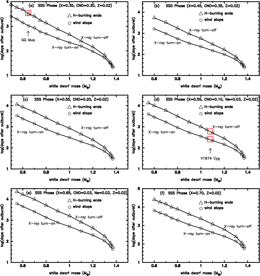
Figure 3.— The turn-on (circles) and turnoff (triangles) times of supersoft X-ray are plotted against the WD mass. X-ray turn-on corresponds to the epoch when optically thick winds stop while X-ray turnoff corresponds to the epoch when hydrogen shell-burning ends. A total of 72 cases are plotted for six different chemical compositions: $(a)$ case CO 2 in Table 2, a large square indicates the epoch of supersoft X-ray turnoff for GQ Mus 1983 (Shanley et al., 1995); $(b)$ case CO 3; $(c)$ case CO 4; $(d)$ case Ne 2, two large squares indicate the epochs of supersoft X-ray turn-on and turnoff for V1974 Cyg 1992 (Krautter et al., 1996); $(e)$ case Ne 3; $(f)$ solar composition.

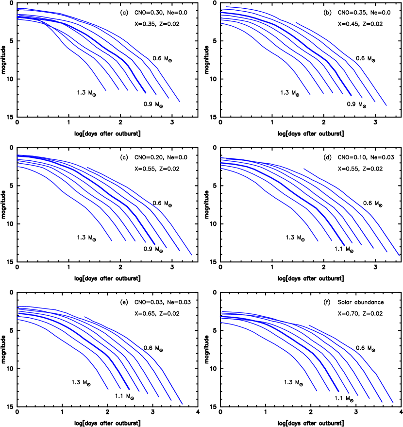
Figure 4.— Calculated light curves for free-free emission during the optically thick wind phase. $(a)$ case CO 2 in Table 2, $(b)$ case CO 3, $(c)$ case CO 4, $(d)$ case Ne 2, $(e)$ case Ne 3, $(f)$ solar composition. Each panel shows light curves for different WD masses, i.e., $M_{\rm WD}=1.3$, 1.2, 1.1, 1.0, 0.9, 0.8, 0.7, and $0.6~{}M_{\sun}$ from left to right. The apparent magnitude constant is set to be $c_{\lambda}=2.5$.

2.3. Nova light curves for free-free emission

The blackbody light curves do not well reproduce the observed visual light curves of novae as already discussed by Hachisu & Kato (2005). Instead these authors have made light curves for free-free emission from optically thin ejecta outside the photosphere that can be reasonably fitted with the optical light curve of V1974 Cyg (catalog ) 1992. Thus, the above authors conclude that, except a very early phase of the outburst, optical fluxes of novae are dominated by free-free emission of the optically thin ejecta as illustrated in Figure 2.

The flux of free-free emission (thermal bremsstrahlung) is

$$j_{\nu}d\Omega dVdtd\nu={{16}\over 3}\left({{\pi}\over 6}\right)^{1/2}{{e^{6}Z^{2}}\over{c^{3}m_{e}^{2}}}\left({{m_{e}}\over{kT_{e}}}\right)^{1/2}~{}g~{}\exp\left(-{{h\nu}\over{kT_{e}}}\right)N_{e}N_{i}d\Omega dVdtd\nu,$$ (8)

where $j_{\nu}$ is the emissivity at the frequency $\nu$, $\Omega$ is the solid angle, $V$ is the volume, $t$ is the time, $e$ is the electron charge, $Z$ is the ion charge in units of $e$, $c$ is the speed of light, $m_{e}$ the electron mass, $k$ is the Boltzmann constant, $T_{e}$ the electron temperature, $g$ is the Gaunt factor, $h$ the Planck constant, and $N_{e}$ and $N_{i}$ are the number densities of electrons and ions (Allen, 1981, p.103).

The electron temperatures of nova ejecta were suggested to be around $T_{e}\sim 10^{4}$ K and almost constant during the nova outbursts (e.g., Ennis et al., 1977, for V1500 Cyg (catalog )). If we further assume that the ionization degree of ejecta is constant during the outburst, we have a flux of

$$F_{\lambda}\propto\int N_{e}N_{i}dV\propto\int_{R_{\rm ph}}^{\infty}{\dot{M}_{\rm wind}^{2}\over{v_{\rm wind}^{2}r^{4}}}r^{2}dr\propto{\dot{M}_{\rm wind}^{2}\over{v_{\rm ph}^{2}R_{\rm ph}}}$$ (9)

for free-free emission of the optically thin ejecta during the optically thick wind phase, where $F_{\lambda}$ is the flux at the wavelength $\lambda$, $N_{e}\propto\rho_{\rm wind}$ and $N_{i}\propto\rho_{\rm wind}$. Here, we assume $v_{\rm wind}=v_{\rm ph}$ and use the relation of continuity, $\rho_{\rm wind}=\dot{M}_{\rm wind}/4\pi r^{2}v_{\rm wind}$, where $\rho_{\rm wind}$ and $v_{\rm wind}$ are the density and velocity of the wind, respectively. We have obtained the absolute magnitude for free-free emission by

$$M_{\lambda}=-2.5\log\left({\dot{M}_{\rm wind}\over{10^{-4}M_{\sun}{\rm yr}^{-1}}}\right)^{2}\left({v_{\rm ph}\over{1000~{}{\rm km~{}s}^{-1}}}\right)^{-2}\left({R_{\rm ph}\over R_{\sun}}\right)^{-1}+C_{\lambda},$$ (10)

or the apparent magnitude by

$$m_{\lambda}=-2.5\log\left({\dot{M}_{\rm wind}\over{10^{-4}M_{\sun}{\rm yr}^{-1}}}\right)^{2}\left({v_{\rm ph}\over{1000~{}{\rm km~{}s}^{-1}}}\right)^{-2}\left({R_{\rm ph}\over R_{\sun}}\right)^{-1}+c_{\lambda},$$ (11)

where $M_{\lambda}$ ($m_{\lambda}$) is the absolute (apparent) magnitude for free-free emission at the wavelength $\lambda$, and $C_{\lambda}$ ($c_{\lambda}$) is a constant. Subtracting equation (10) from equation (11), we have

$$c_{\lambda}=(m-M)_{\lambda}+C_{\lambda},$$ (12)

where $(m-M)_{\lambda}$ is the apparent distance modulus. In the present paper, we call $c_{\lambda}$ the apparent magnitude constant. We cannot uniquely specify the constant, $C_{\lambda}$ (or $c_{\lambda}$), because radiative transfer is not calculated outside the photosphere. Instead we choose the constant to fit the light curve.

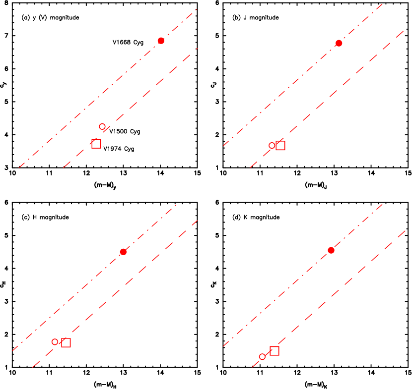
Figure 5.— The apparent magnitude constant, $c_{\lambda}$, in eq. (11) is plotted against the apparent distance modulus, $(m-M)_{\lambda}$, for three novae, V1500 Cyg (Open circle), V1668 Cyg (filled circle), and V1974 Cyg (open square). Each panel shows $(a)$ $y$ (or $V$), $(b)$ $J$, $(c)$ $H$, and $(d)$ $K$ bands. Dash-dotted line: eq. (12) for V1668 Cyg. Dashed line: eq. (12) both for V1500 Cyg and V1974 Cyg.

Figure 4 shows the free-free light curves calculated from equation (11) with a fixed value of $c_{\lambda}=2.5$ for the six cases in Table 2. Here we plot the light curves only during the optically thick wind phase. The wind stops at the lower edge of each line. It is clear that the heavier the WD mass is the faster the development of a nova light curve is. Thus we conclude that the nova speed class is in principal closely related to the WD mass even when free-free emission dominates the nova optical fluxes.

Using the individual fitting results described below in §3, 4, and 5, we plot the apparent magnitude constant, $c_{\lambda}$, against the apparent distance modulus, $(m-M)_{\lambda}$, each for the $y$ (or $V$), $J$, $H$, and $K$ bands in Figure 5. If these three novae are just on a straight line with a slope of unity, we may conclude that the constant $C_{\lambda}$ for the absolute magnitude is universal among various novae. However, $C_{\lambda}$ for V1668 Cyg (catalog ) is about $1.0-1.4$ mag dimmer than that for V1500 Cyg (catalog ) and V1974 Cyg (catalog ). Each nova probably has a different $C_{\lambda}$, although we cannot draw any firm statements from only three novae.

The distance modulus is calculated from

$$(m-M)_{\lambda}=5+5\log d+A_{\lambda},$$ (13)

where $d$ is the distance to the object. Absorption law for each band is given by $A_{y}=A_{V}=3.1E(B-V)$ for $y$ and $V$, $A_{J}=0.87E(B-V)$ for $J$, $A_{H}=0.54E(B-V)$ for $H$, $A_{K}=0.35E(B-V)$ for $K$, and $A_{L}=0.18E(B-V)$ for $L$ band (e.g., Rieke & Lebofsky, 1985).

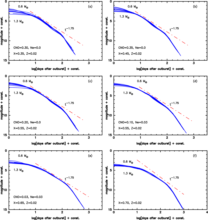
Figure 6.— Same as those for Fig. 4, but each light curve is shifted vertically and horizontally to show a universal decline law. We can see a break on the free-free emission light curves near 100 days after outburst (200 days after outburst for the solar composition). We define this time as $t_{\rm break}$.

2.4. Template light curve of classical novae

We have found that the free-free light curves calculated for various WD masses are quite homologous and overlap with each other as shown in Figure 6. Here we shift each light curve up and down and back and forth to overlap it with the $1.0~{}M_{\sun}$ WD model, which is fixed in the figure. Table 9 lists the horizontal shifts in the $m_{\lambda}-\log t$ plane that correspond to a time scaling factor of the light curve.

Figure 7 shows that the $1.0~{}M_{\sun}$ WD models with different chemical compositions are also homologous and can be overlapped with each other in the $m_{\lambda}-\log t$ plane except for the solar composition. Thus we may conclude that all these five light curves are homologous independently of the WD mass or the chemical composition. Only the solar composition model shows a bit smaller decline in the $m_{\lambda}-\log t$ plane. We call this property “a universal decline law of classical novae.” Once a template light curve is given, we can specify a nova light curve using only one parameter and we choose the time at the “knee” as such a parameter. The template light curve has a prominent knee at $\log t\approx 2$ ($t\sim 100$ days after outburst) in Figure 7b, which is the only parameter that characterizes the timescale of nova light curves. This break time, $t_{\rm break}$, is listed in Table 10 for each set of the WD mass and chemical composition.

It should be noted that this universal decline rate, $\alpha=1.7-1.75$ (here, $F_{\lambda}\propto t^{-\alpha}$, $t$ is the time in days after outburst), yields a simple relation between $t_{2}$ and $t_{3}$, where $t_{2}$ is the time in days during which the star decays by 2 mag from the optical maximum and $t_{3}$ is the time in days in 3 mag decay from the optical maximum. Since the flux obeys $F_{\lambda}\propto t^{-\alpha}$ before the break, we have

$$m_{\lambda}=-2.5\log F_{\lambda}+{\rm const.}=2.5\alpha\log t+{\rm const.}$$ (14)

The decay parameters of light curves, $t_{2}$ and $t_{3}$, are related to the parameter $\alpha$ as

$$1=2.5\alpha\left[\log(t_{3}+\Delta t_{0})-\log(t_{2}+\Delta t_{0})\right],$$ (15)

where $\Delta t_{0}$ is the time in days from the outburst to the optical maximum. If $\alpha=1.75$, we have

$$t_{3}=1.69~{}t_{2}+0.69~{}\Delta t_{0}.$$ (16)

Since the rise time $\Delta t_{0}$ is usually short, from a few days (fast novae) to several days (moderately fast novae), the relation between $t_{2}$ and $t_{3}$ is very consistent with an (observational) empirical relation

$$t_{3}=(1.68\pm 0.08)~{}t_{2}+(1.9\pm 1.5){\rm~{}days},{\rm~{}for~{}}t_{3}<80{\rm~{}days}$$ (17)

or

$$t_{3}=(1.68\pm 0.04)~{}t_{2}+(2.3\pm 1.6){\rm~{}days},{\rm~{}for~{}}t_{3}>80{\rm~{}days},$$ (18)

given by Capaccioli et al. (1990).

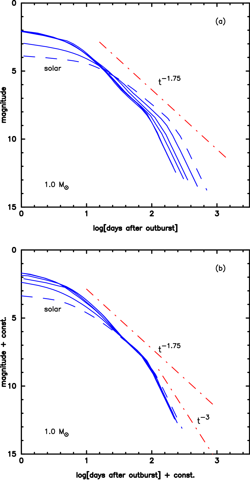
Figure 7.— $(a)$ Theoretical free-free light curves for the $1.0~{}M_{\sun}$ WDs with six different chemical compositions. $(b)$ The above six light curves are shifted vertically and horizontally to be overlapped with each other. Only the case of solar abundance (dashed line labeled by “solar”) is somewhat different from the other five cases. We can see a break on the free-free emission light curves near 100 days after outburst from a slope of $\sim t^{-1.75}$ to $\sim t^{-3.5}$.

Figure 8.— The ultraviolet (UV) 1455Å  and free-free emission light curves during the wind phase for six different chemical compositions: $(a)$ case CO 2, $(b)$ case CO 3, $(c)$ case CO 4, $(d)$ case Ne 2, $(e)$ case Ne 3, and $(f)$ the solar composition. Eight light curves for different WD masses are calculated in each panel, i.e., $M_{\rm WD}=1.3$, 1.2, 1.1, 1.0, 0.9, 0.8, 0.7, and $0.6~{}M_{\sun}$ from left to right. The horizontal timescale is linear (not logarithmic) but stretched or squeezed to overlap each other. This time scaling factor is the same as those in Table 9. The magnitudes of free-free light curves are arbitrary shifted to overlap with each other. The vertical flux scale for the UV 1455Å  is linear and normalized by the maximum flux.

Table 9Time scaling factor of the nova light curves

WD mass	CO 2	CO 3	CO 4	Ne 2	Ne 3	solar
($M_{\sun}$)
0.60	0.65	0.70	0.76	0.79	0.82	0.87
0.70	0.47	0.50	0.57	0.57	0.60	0.60
0.80	0.30	0.32	0.33	0.33	0.36	0.34
0.90	0.12	0.14	0.13	0.14	0.14	0.14
1.00	0.00	0.00	0.00	0.00	0.00	0.00
1.10	$-0.20$	$-0.17$	$-0.21$	$-0.17$	$-0.17$	$-0.22$
1.20	$-0.40$	$-0.35$	$-0.39$	$-0.34$	$-0.34$	$-0.41$
1.30	$-0.64$	$-0.62$	$-0.67$	$-0.61$	$-0.62$	$-0.66$

Table 10Time at the break for the free-free emission light curves

WD mass	CO 2	CO 3	CO 4	Ne 2	Ne 3	solar
($M_{\sun}$)	(days)	(days)	(days)	(days)	(days)	(days)
0.60	390	436	616	812	1120	1510
0.70	257	275	398	490	676	832
0.80	174	182	229	282	389	457
0.90	114	120	145	182	234	288
1.00	87	87	107	132	169	209
1.10	55	59	66	89	115	126
1.20	35	39	44	60	78	81
1.30	20	21	23	32	41	46

Figure 9.— Four typical nova timescales are plotted against the WD mass for six different chemical compositions of the nova envelope. Each panel shows $(a)$ $t_{\rm H-burning}$, the time when hydrogen burning ends, $(b)$ $t_{\rm wind}$, the time when optically thick winds stop, $(c)$ $\Delta t_{\rm UV,FWHM}$, the UV 1455Å  duration defined by the full width at the half maximum, and $(d)$ $t_{\rm break}$, the time of break. These timescales depend not only on the WD mass but also on the chemical composition.

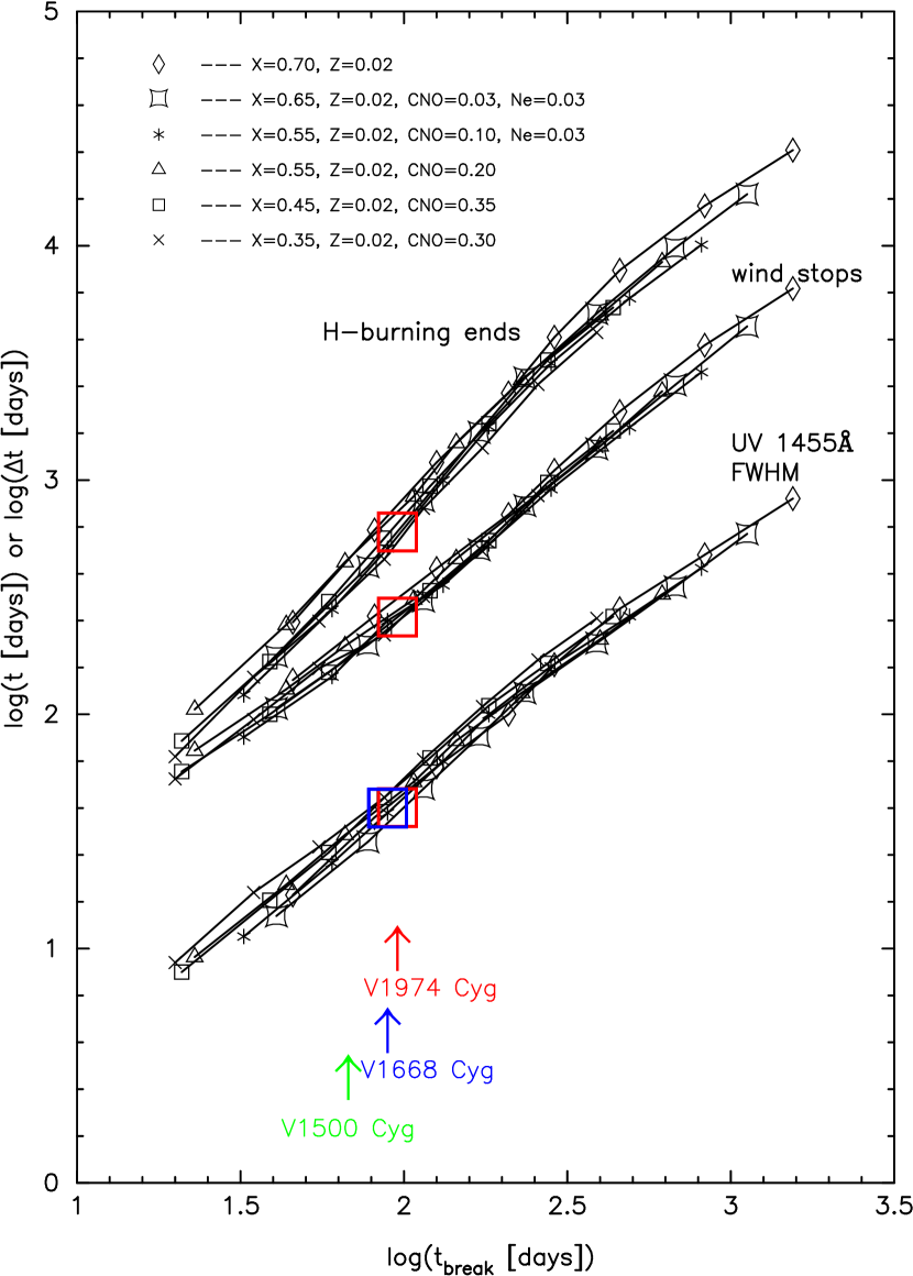
Figure 10.— Three typical nova timescales of $t_{\rm H-burning}$, $t_{\rm wind}$, and $\Delta t_{\rm UV,FWHM}$ are plotted against $t_{\rm break}$. These three timescales are monotonic functions of $t_{\rm break}$, so we can predict the epochs of $t_{\rm H-burning}$ and $t_{\rm wind}$ if $t_{\rm break}$ is observationally determined. Estimated values of $t_{\rm break}$ are indicated by arrows for V1500 Cyg, V1668 Cyg, and V1974 Cyg. Large open squares denote the corresponding timescales determined from the observations.

2.5. UV 1455 Å  light curve

Cassatella et al. (2002) adopted two UV continuum bands to describe the UV fluxes of classical novae based on the IUE observation. One is the UV 1455 Å  band with a 20 Å  width (centered on 1455 Å  ) and the other is the UV 2885 Å  band with a 20 Å  width (centered on 2885 Å  ). Both of the bands are selected to avoid prominent emission or absorption lines in the UV spectra. In our blackbody light curve model, the UV 1455 Å  flux reaches its maximum at a photospheric temperature of $\sim 27,000$ K while the UV 2885 Å  band reaches its maximum at a lower photospheric temperature of $\sim 13,000$ K.

In this paper, we adopt only the UV 1455 Å  band because our blackbody light curve model for the UV 1455 Å  band nicely follows the UV flux near the temperature of $\sim 27,000$ K. This is confirmed partly by the theoretical nova spectra calculated by Hauschildt et al. (1995). They showed non-LTE spectra ranging from optical to UV in their Figure 3. Their UV 1455 Å band region is well fitted with a blackbody spectrum of $T_{\rm eff}=25,000$ K, around which our UV 1455 Å  flux reaches its maximum. This suggests that the blackbody light curve model for the 1455 Å  band is a good approximation to the nova UV flux near its flux maximum. This is observationally confirmed by direct fittings with the IUE observation for V1668 Cyg (catalog ) in §4 and for V1974 Cyg (catalog ) in §5.

On the other hand, our blackbody light curve model for the UV 2885 Å  band is not a good approximation to the nova UV flux at/near its maximum partly because our blackbody 2885 Å  flux is about two times larger than the UV flux calculated by Hauschildt et al. (1995) at $T_{\rm eff}=10,000$ K, near which the 2885 Å  flux reaches its maximum. To summarize, avoiding strong emission/absorption lines, we use the 1455 Å  band as a UV evolution of a classical nova, which is accidentally well followed by the blackbody light curve model near its flux maximum.

Our light curves of the UV 1455 Å  band are plotted together with the free-free emission light curves in Figure 8 for various WD masses and chemical compositions. Note that the horizontal axis is not logarithmic but linear in this figure. These are stretched or squeezed by the same factor tabulated in Table 9. Light curves almost overlap with each other. Therefore, we may conclude that the UV 1455 Å  light curve is also specified by only one parameter, such as a time scaling factor or $t_{\rm break}$.

2.6. Relations among various nova timescales

Figure 9 shows the various timescales that characterize nova outbursts: $(a)$ $t_{\rm H-burning}$, the epoch when hydrogen shell-burning ends; $(b)$ $t_{\rm wind}$, the epoch when optically thick winds stop; and $(c)$ $\Delta t_{\rm UV,FWHM}$, the UV 1455 Å  duration, which is properly defined by the full width at the half maximum (FWHM) of the UV 1455 Å  light curve. In addition to these three timescales, it shows $(d)$ the time of break, $t_{\rm break}$, where the free-free light curve has a knee in the $m_{\lambda}-\log t$ plane. It is clear that these timescales depend not only on the WD mass but also on the chemical composition.

Figure 10 shows the first three timescales, $t_{\rm H-burning}$, $t_{\rm wind}$, and $\Delta t_{\rm UV,FWHM}$ against the last one, $t_{\rm break}$. Now these three former timescales are monotonic functions of $t_{\rm break}$, regardless of the WD mass or the chemical composition. Therefore, once we determine $t_{\rm break}$ from observations, we can predict the duration of a luminous supersoft X-ray phase of a nova, i.e., its turn-on ($t_{\rm wind}$) and turnoff ($t_{\rm H-burning}$) times. We have added the corresponding epochs for three individual novae, V1500 Cyg (catalog ), V1668 Cyg (catalog ), and V1974 Cyg (catalog ).

2.7. Transition in classical nova light curves

Figure 11 shows a schematic light curve of the free-free emission. The early slope of $F_{\lambda}\propto t^{-1.75}$ changes at $t_{\rm break}$ to the late slope of $F_{\lambda}\propto t^{-3.5}$. This break occurs a bit before the wind stops. This change of slope is caused mainly by a sharp decrease in the wind mass-loss rate, $\dot{M}_{\rm wind}$, together with an increase in the wind velocity, $v_{\rm ph}$.

After the optically thick wind stops, the free-free emission light curve changes its decline rate because no additional mass is supplied to the ejecta. In such a case, the free-free flux can be roughly estimated as

$$F_{\lambda}\propto\int N_{e}N_{i}dV\propto\rho^{2}V\propto{M_{\rm ej}^{2}\over V^{2}}V~{}\propto R^{-3}\propto t^{-3},$$ (19)

(e.g., Woodward et al., 1997), where $\rho$ is the density, $M_{\rm ej}$ is the ejecta mass ($M_{\rm ej}$ is constant in time after the wind stops), $R$ is the radius of the ejecta ($V\propto R^{3}$), and $t$ is the time after the outburst. Therefore, in the later phase, the free-free flux decays as $t^{-3}$. In the actual case, the transition from $t^{-3.5}$ to $t^{-3}$ may occur just before the wind stops.

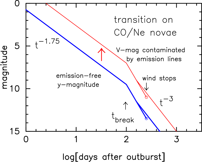
Figure 11.— A schematic nova light curve for our free-free emission model. When strong emission lines such as [O III] emission lines begin to contribute to the nova light curve, its light curve is gradually lift up (thin solid) from our template nova light curve (thick solid). This occurs when the nova enters a nebular phase. We recommend observations with narrower band filters such as the Strömgren $y$ band to accurately follow the continuum flux even in the nebular phase.

3. V1500 Cyg (Nova Cygni 1975)

We will examine now individual novae. The first example is an extremely fast nova V1500 Cyg (catalog ). It has probably the fastest and largest eruption among novae. It rose to a maximum of $m_{V}=1.85$ on 1975 August 31 from a preoutburst brightness of $m_{V}>21$ (Young et al., 1976). A distance of $1.2\pm 0.2$ kpc (Lance et al., 1988) and an interstellar extinction of $E(B-V)=0.5\pm 0.05$ (Ferland, 1977) suggest a peak absolute luminosity of $M_{V}=-10.0\pm 0.3$, which is about 4 mag brighter than the Eddington luminosity for a $1.0~{}M_{\odot}$ WD (see, e.g., eq. (4) of Hachisu & Kato, 2004, for the Eddington $V$ magnitude). An extensive summary of the observational results and modelings can be found in the review by Ferland et al. (1986).

3.1. Light curve fitting in the decay phase

Gallagher & Ney (1976) obtained the magnitudes of the three broad optical $V$, $R$, and $I$ bands and the eight infrared 1.2, 1.6, 2.2, 3.6, 4.8, 8.5, 10.6, and $12.5~{}\mu$m bands during the 50 days following the discovery. They estimated the outburst day to be August 28.9 UT from the data of angular expansion of the photosphere. They conclude that the spectrum energy distribution is approximately that of a blackbody during the first 3 days while it is close to $F_{\nu}=$ constant after the fourth day. This $F_{\nu}=$ constant spectra resemble those usually ascribed to the free-free emission.

Based on the infrared photometry from 1 to $20~{}\mu$m, Ennis et al. (1977) also presented similar observational results like those of Gallagher & Ney (1976). The nova spectrum changed from a blackbody to a bremsstrahlung emission at day $\sim 4-5$, that is, from that of a Rayleigh-Jeans ($F_{\nu}\propto\nu^{2}$) to that of a thermal bremsstrahlung emission ($F_{\nu}\sim$ constant). Thus we regard that the nova enters a phase, in which free-free emission dominates, about 5 days after the outburst.

They also obtained the onset of outburst on JD 2,442,653.0$\pm 0.5$ from an analysis of the photospheric expansion similar to that by Gallagher & Ney (1976). Therefore we define the outburst day of V1500 Cyg as JD 2,442,653.0 ($t=0$) in our model.

Figure 12 shows the $y$ magnitude light curve observed by Lockwood & Millis (1976) together with the three near-IR $J$ (1.2 $\mu$m), $H$ (1.6 $\mu$m), and $K$ (2.2 $\mu$m) magnitudes (Gallagher & Ney, 1976; Kawara et al., 1976; Ennis et al., 1977). We have measured the time of “knee” on these four light curves and obtained an average value of $t_{\rm break}\sim 70$ days after the outburst. This value indicates a WD mass of $1.15~{}M_{\sun}$ among $1.1$, 1.15, and $1.2~{}M_{\sun}$ WDs (see Table 10). Here we assume chemical composition of $X=0.55$, $X_{\rm CNO}=0.10$, $X_{\rm Ne}=0.03$, and $Z=0.02$ (case Ne 2 in Table 2), which is close to the estimate given by Lance et al. (1988) as tabulated in Table 1.

Our best-fit model closely follows all the observations of optical $y$ and infrared $J$, $H$, and $K$ bands during the period from several to $\sim 100$ days after the outburst as seen in Figure 12. We have obtained $c_{y}=4.25$, $c_{J}=1.67$, $c_{H}=1.77$, and $c_{K}=1.32$ to fit with the V1500 Cyg (catalog ) light curves as already introduced in Figure 5. These well-fitted results confirm that free-free emission dominates the optical and infrared continuum at least from several days to $\sim 100$ days after the outburst.

Figure 12d also shows the light curve model by Ennis et al. (1977). They assumed an expanding shell with an initial thickness of $H$ and the velocity of $v$. Then the time dependence of the flux is approximately given by

$$F_{\nu}\propto t^{-2}\left(1+2c_{s}t/H\right)^{-1}.$$ (20)

In early stages of the expansion, the flux will be proportional to $t^{-2}$, while it is more close to $t^{-3}$ in later times. They assumed a temperature of 10,000 K that gives a sound velocity of $c_{s}\sim 10$ km s^-1. The transition at $\sim 60$ days between the two slopes derives $H\sim 10^{13}$ cm, which indicates a shell-ejection duration of a half day after the explosion with an expansion velocity of $v\sim 2000$ km s^-1. The resultant light curve is not so closely following the observational data compared with that of our best-fit model.

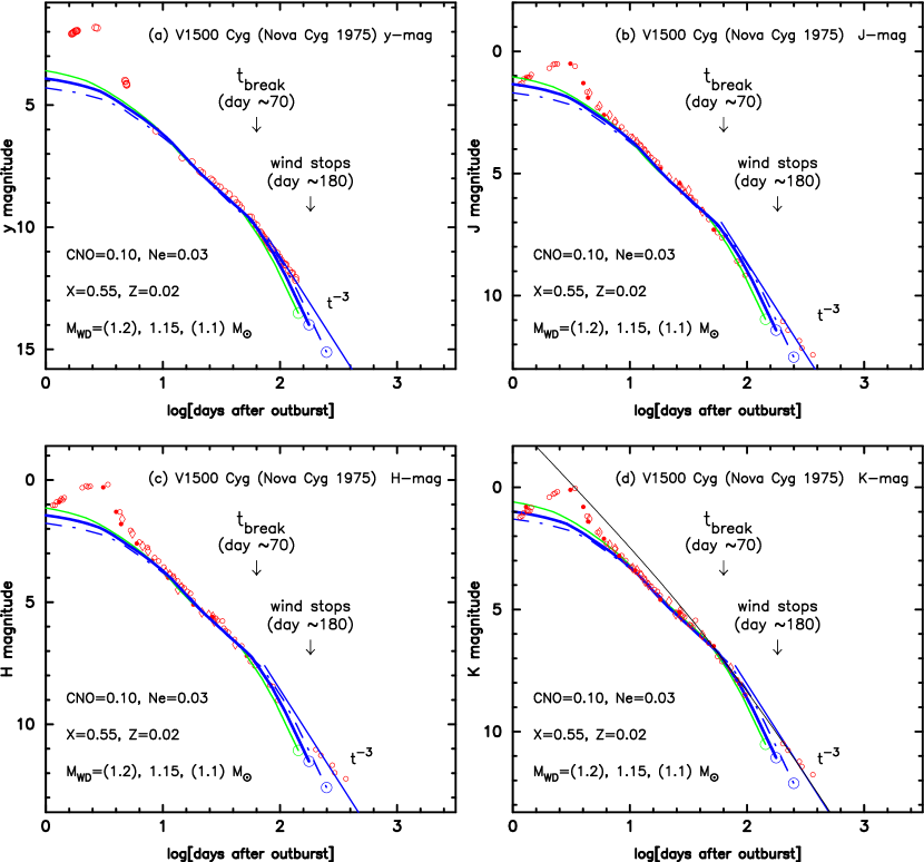
Figure 12.— Calculated free-free light curves are plotted for the three WD mass models: $1.1~{}M_{\sun}$ (dash-dotted line), $1.15~{}M_{\sun}$ (thick solid line), and $1.2~{}M_{\sun}$ (medium thickness solid line). Our free-free light curves nicely follow the observation after day $\sim 5$ as suggested by Ennis et al. (1977). Comparing $t_{\rm break}$ with the observation, we choose the $1.15~{}M_{\sun}$ model among the $1.1$, $1.15$, and $1.2~{}M_{\sun}$ models (see Table 10). We also added light curves of $F_{\lambda}\propto t^{-3}$ after the optically thick wind stops. Here we assume a chemical composition of $X=0.55$, $X_{\rm CNO}=0.10$, $X_{\rm Ne}=0.03$, and $Z=0.02$ (case Ne 2 in Table 2). Each panel shows $(a)$ $y$ magnitude (open circle: Lockwood & Millis, 1976). $(b)$ $J$, $(c)$ $H$, and $(d)$ $K$ magnitudes. The data of near infrared $J$, $H$, and $K$ bands are taken from Ennis et al. (1977, open circles), Kawara et al. (1976, open diamonds), and Gallagher & Ney (1976, filled circles). Thin solid line in $(d)$: a model light curve of eq.(20) proposed by Ennis et al. (1977).

The wide-band $V$ magnitude observations are plotted in Figure 13. In general, the wide-band $V$ magnitude suffers from contamination of strong emission lines especially in the nebular phase. Comparing with Figure 12a, we see that the $V$ magnitude decays a little bit more slowly than the $y$ magnitude does during $10<t<100$ days. This is due to the appearance of strong [O III] 4958.9 and 5006.9 Å  emission lines located just at the shorter edge of the $V$ bandpass. We see some systematic differences even in the three different $V$ magnitudes among open squares (Arkhipova & Zaitseva, 1976), open diamonds (Pfau, 1976), and open circles (Tempesti, 1979). This comes from the difference of the wavelength sensitivity among these three $V$ systems near the shorter edge of the $V$ bandpass. Although the visual magnitudes are the richest in observational points as shown in Figure 13, the difference from the $y$ band (even from the $V$ band) becomes significant in the later nebular phase. Therefore we use the medium-band $y$ magnitude for the optical light curve fitting. We must be careful that the $V$ magnitude light curves do not precisely follow the continuum flux but are highly contaminated by strong emission lines especially in later phases.

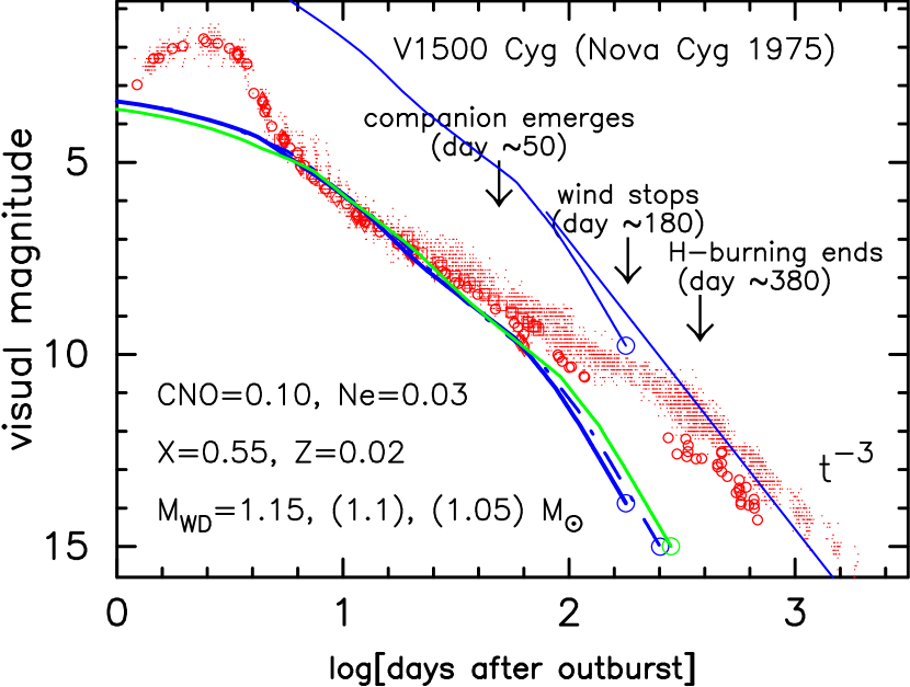
Figure 13.— Same as Fig. 12, but for the visual and $V$ observations. Our model light curves are plotted for the three WD masses of $1.15$ (thick solid), 1.1 (dash-dotted), and $1.05~{}M_{\sun}$ (thin solid). The visual observational data are taken from AAVSO (small dots) and the $V$ data are taken from Tempesti (1979, open circles), Pfau (1976, open diamonds), and Arkhipova & Zaitseva (1976, open squares). Three epochs are indicated by arrows for our best-fit $1.15~{}M_{\sun}$ model.

3.2. Distance to V1500 Cyg

The distance to V1500 Cyg (catalog ) has been discussed by many authors. Young et al. (1976) estimated the distance to be $1.4\pm 0.1$ kpc for $E(B-V)=0.45$ (Tomkin et al., 1976) from the reddening-distance law toward the nova, which is shown in Figure 14. The data align almost in a straight line. Another estimate comes from an empirical relation between the maximum absolute magnitude and the rate of decline (MMRD). Using Schmidt-Kaler’s (Schmidt, 1957) empirical relation

$$M_{V,{\rm max}}=-11.5+2.5\log t_{3},$$ (21)

we obtain $M_{V,{\rm max}}\approx-10.11$ together with $t_{3}=3.6$ days (e.g. Duerbeck & Wolf, 1977). Combining the maximum apparent magnitude of $m_{V,{\rm max}}=1.85$ and the absolute maximum magnitude of $M_{V,{\rm max}}=-10.11$, we obtain a simple relation of

$$(m-M)_{V}=5+5\log d+3.1E(B-V)=11.96.$$ (22)

This distance-reddening relation is plotted in Figure 14, which is labeled “MMRD.”

A firm upper limit to the apparent distance modulus was obtained to be $(m-M)_{V}\leq 12.5$ by Ando & Yamashita (1976) from the Galactic rotational velocities of interstellar H and K absorption lines. This upper limit is also plotted in Figure 14, which is labeled “AY.”

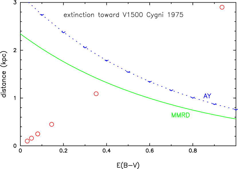
Figure 14.— The distance-reddening law in the direction of V1500 Cyg, each star (open circles) of which is taken from Young et al. (1976). Solid line: maximum magnitude versus rate of decline relation (labeled “MMRD”). Dotted line with reverse carets: upper limit to $(m-M)_{V}$ derived by Ando & Yamashita (1976).

The nebular expansion parallax method is a different way to estimate the distance. Becker & Duerbeck (1980) first imaged an expanding nebular ($0\farcs 25$ yr^-1) of V1500 Cyg (catalog ) and estimated the distance to be 1350 pc together with an expansion velocity of $v_{\rm exp}=1600$ km s^-1. However, Wade et al. (1991) resolved an expanding nebular and obtained a much lower expansion rate of $0\farcs 16$ yr^-1. Using a much smaller expansion velocity of $v_{\rm exp}=1180$ km s^-1 observed by Cohen (1985), they estimated the distance to be 1.56 kpc. Finally, Slavin et al. (1995) obtained a more expanding image of the nebular ($0\farcs 16$ yr^-1) and determined the distance to be 1550 pc assuming $v_{\rm exp}=1180$ km s^-1.

Therefore we may conclude that the distance is $d\approx 1.5$ kpc assuming a color excess of $E(B-V)\approx 0.45$ as shown in Figure 14. Using this distance of $d\approx 1.5$ kpc and color excess of $E(B-V)\approx 0.45$, we have estimated the apparent distance moduli of $(m-M)_{\lambda}$ for the $y$, $J$, $H$, and $K$ bands, as already introduced in Figure 5.

3.3. The white dwarf mass

The WD mass of $1.15~{}M_{\sun}$ for our best-fit model is consistent with $M_{\rm WD}>0.9~{}M_{\sun}$ obtained by Horne and Schneider (1989), based on a spectral line analysis. Such a massive WD is considered to be an oxygen-neon-magnesium (ONeMg) WD. Umeda et al. (1999) obtained an upper limit for the mass of a CO WD in a binary, $M_{\rm CO}\lesssim 1.07~{}M_{\sun}$, when it is just born. The WD mass decreases after every nova outburst because a part of the WD core is dredged up by convection and blown off during the outburst (e.g., Prialnik & Kovetz, 1995). Therefore, the $1.15~{}M_{\sun}$ WD is probably not a CO WD but an ONeMg WD. This conclusion is also consistent with the chemical composition of the ejecta as tabulated in Table 1 (Ferland & Shields, 1978; Lance et al., 1988).

3.4. Emergence of the secondary component

The mass of the donor star (the secondary component) can be estimated from the orbital period. Semeniuk et al. (1995) determined an orbital period of $P_{\rm orb}=0.1396$ days ($3.351$ hr) from the orbital modulations with an amplitude of $\sim 1$ mag. Using Warner’s (1995) empirical formula

$${{M_{2}}\over{M_{\sun}}}\approx 0.065\left({{P_{\rm orb}}\over{\rm hours}}\right)^{5/4},\mbox{~{}for~{}}1.3<{{P_{\rm orb}}\over{\rm hours}}<9$$ (23)

we have $M_{2}=0.29~{}M_{\sun}$. Then the separation is $a=1.28~{}R_{\sun}$, the effective radius of the Roche lobe for the primary component (WD) is $R_{1}^{*}=0.64~{}R_{\sun}$, and the effective radius of the secondary is $R_{2}^{*}=0.34~{}R_{\sun}$. In our model, the companion emerges from the WD envelope when the photospheric radius of the WD shrinks to $R_{\rm ph}\sim 1.0~{}R_{\sun}$ (see Fig. 1). This epoch is about day 50 in our best-fit model of $M_{\rm WD}=1.15~{}M_{\sun}$, but this time there is no transition of any kind in the optical light curve.

4. V1668 Cyg (Nova Cygni 1978)

V1668 Cyg (catalog ) was discovered on September 10.24 UT, 1978 (Morrison, 1978), 2 days before its optical maximum of $m_{V,{\rm max}}=6.04$. Since no estimate of the outburst day has ever been given, we assume it to be JD 2,443,759.0. The outburst of V1668 Cyg (catalog ) was well observed with IUE in the ultraviolet (UV) during a full period of the UV outburst (e.g., Cassatella et al., 1979; Stickland et al., 1981). In a pioneering work of a nova light-curve model, Kato (1994) presented light curve fitting of V1668 Cyg based on the blackbody model. However, it is too simplified for classical novae. Here we present new light curves for the optical and IR observations based on the free-free emission model.

4.1. UV 1455 Å  fluxes

Figure 15 shows light curve fitting of our UV 1455Å  flux with the IUE data (Cassatella et al., 2002). Here we adopt a chemical composition of $X=0.45$, $X_{\rm CNO}=0.35$, and $Z=0.02$ (case CO 3 in Table 2) after Stickland et al. (1981) and Andreä et al. (1994). Regarding the steep fall of the UV flux on JD 2,443,815 as caused by a dust absorption, we choose the best-fit model of $M_{\rm WD}=0.95~{}M_{\sun}$ among 0.9, 0.95, and $1.0~{}M_{\sun}$ WDs. We have to simultaneously fit our model light curves with both the optical and UV 1455 Å  observations as shown in Figures 16.

The chemical composition of the ejecta suggests a CO WD. Our estimated WD mass of $M_{\rm WD}\approx 0.95~{}M_{\sun}$ is consistent with the upper mass limit for a CO WD at its birth in a binary, i.e., $M_{\rm CO}\lesssim 1.07~{}M_{\sun}$ (Umeda et al., 1999).

Figure 15.— UV 1455 Å  light curves for the best-fit $0.95~{}M_{\sun}$ WD model (thick solid line) together with the $1.0~{}M_{\sun}$ (thin solid line labeled by $1.0~{}M_{\sun}$) and $0.9~{}M_{\sun}$ (thin solid line labeled by $0.9~{}M_{\sun}$) WD models. Here we assume a chemical composition of $X=0.45$, $X_{\rm CNO}=0.35$, and $Z=0.02$ (case CO 3 in Table 2). The UV 1455 Å  data (large open circles) are taken from Cassatella et al. (2002). A large part of the UV flux is absorbed by dust after the formation of an optically thin dust shell.

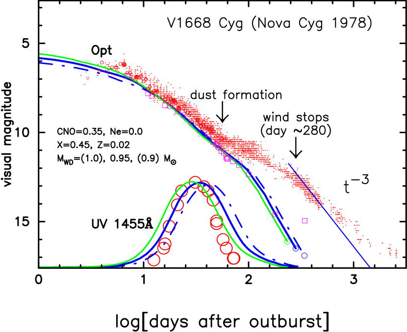
Figure 16.— Free-free emission and UV 1455 Å  light curves for the best-fit $0.95~{}M_{\sun}$ WD model (thick solid line) together with the $1.0~{}M_{\sun}$ (medium thickness solid line) and $0.9~{}M_{\sun}$ (dash-dotted line) WD models. A straight line of $F_{\lambda}\propto t^{-3}$ is also added after the optically thick winds stop. We assume a chemical composition of $X=0.45$, $X_{\rm CNO}=0.35$, and $Z=0.02$ (case CO 3 in Table 2). Visual observation (small dots) is taken from AAVSO. The UV 1455 Å  data (large open circles) are taken from Cassatella et al. (2002). Two epochs are indicated by an arrow: one is the formation epoch of an optically thin dust shell and the other is the epoch when the optically thick winds stop. The $y$ magnitude (open squares: Gallagher et al., 1980b) and $V$ magnitude (small open circles: Mallama & Skillman, 1979) observations are added. It is clear that the $y$ magnitude departs from the visual magnitude after day $\sim 50$.

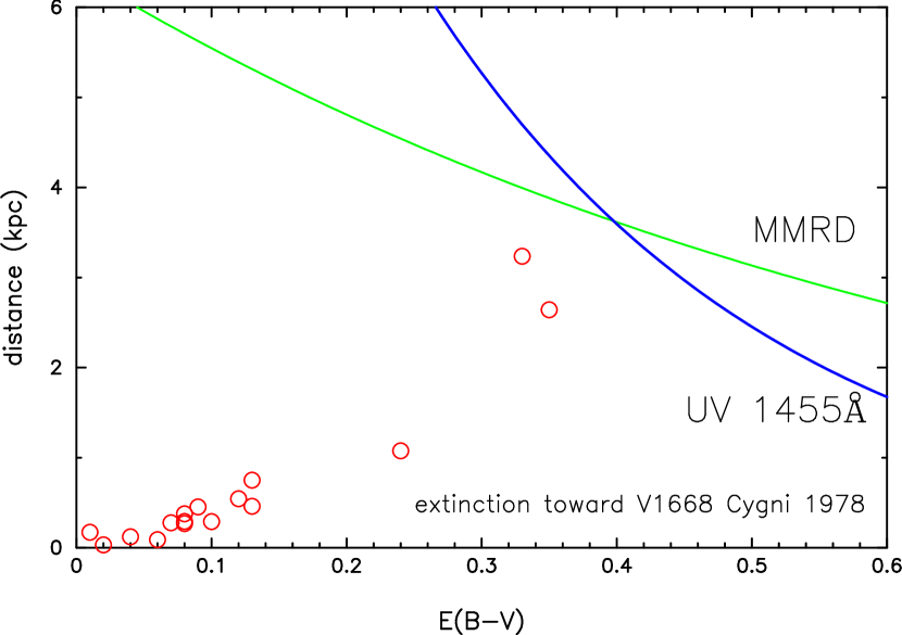
Figure 17.— The distance-reddening law in the direction of V1668 Cyg, each star (open circles) of which is taken from Slovak & Vogt (1979). Solid lines: the distance-reddening relation calculated from the UV 1455Å  flux fitting (labeled “UV 1455 Å”) and the maximum magnitude versus rate of decline relation (labeled “MMRD”). These three trends/lines merge into one at the point of $E(B-V)\approx 0.4$ and $d\approx 3.5$ kpc.

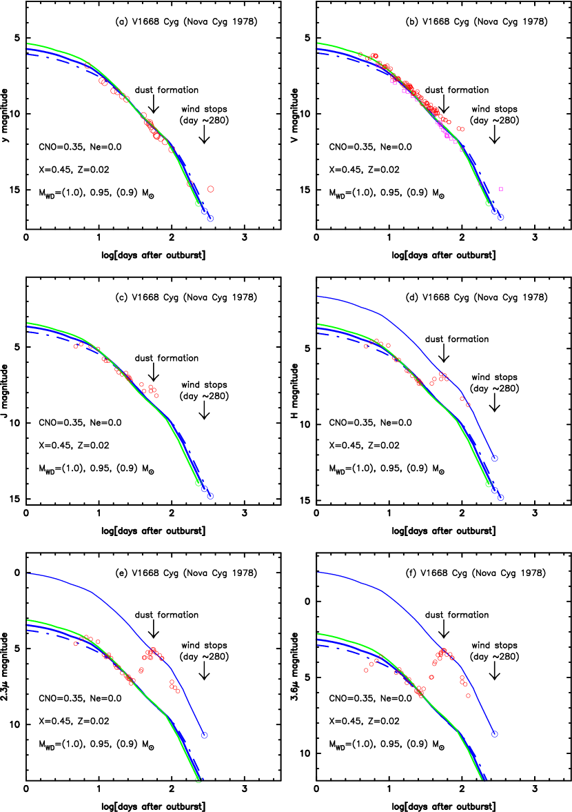
Figure 18.— Free-free light curves for the best-fit $0.95~{}M_{\sun}$ WD model (thick solid line and a lift-up thin solid line) together with the $0.90~{}M_{\sun}$ (dash-dotted) and $1.0~{}M_{\sun}$ (medium thickness solid) WD models. Each panel shows $(a)$ $y$ magnitude (Gallagher et al., 1980b), $(b)$ $V$ magnitude (open circles), data of which are taken from Mallama & Skillman (1979), together with $y$ magnitude (open square), $(c)$ $J$, $(d)$ $H$, $(e)$ $K$ ($2.3\mu$m), and $(f)$ $L$ ($3.6\mu$m) magnitudes. The near infrared data of $J$, $H$, $K$, and $L$ (open circles) are taken from Gehrz et al. (1980). We also added free-free light curves that follow the brightness after the dust formation for the three infrared bands in $(d)$–$(f)$. Two epochs are indicated: one is the epoch when the optically thin dust shell formed and the other is the epoch when the optically thick winds stopped for the $0.95~{}M_{\sun}$ WD model. Large open circles at the lower end of each free-free light curve indicate the epoch when the optically thick winds stop.

4.2. Distance to V1668 Cyg

The distance-reddening law in the direction of V1668 Cyg (catalog ) was obtained by Slovak & Vogt (1979), although the number of stars is small and the data are scattered as shown in Figure 17. They also obtained a reddening of $E(B-V)=0.38$ from the interstellar feature of K I (7699 Å) and then a distance of $d=3.3$ kpc. Duerbeck et al. (1980) criticized Slovak & Vogt’s work and proposed a distance of $d=2.3$ kpc from their newly obtained distance-reddening law and $E(B-V)=0.35$, based on the same stars depicted in Figure 17. Assuming that the optical maximum is the Eddington luminosity, Stickland et al. (1981) estimated the distance to be $d=2.2$ kpc together with their $E(B-V)=0.40$ from the 2200 Å  feature. It is clear that these distance-reddening laws rely only on the three stars beyond 1 kpc in Figure 17. Since no accurate law is drawn from these little data, we cannot judge the results of both Slovak & Vogt (1979) and Duerbeck et al. (1980). As for the result of Stickland et al., we have no evidence that the maximum luminosity of V1668 Cyg (catalog ) is just the Eddington limit.

The distance to the nova can be also estimated from the absolute magnitude at the optical maximum versus rate of decline (MMRD) relation. Klare et al. (1980) obtained $M_{V,{\rm max}}=-8.0\pm 0.2$ from Schmidt-Kaler’s (Schmidt, 1957) relation (21) together with $t_{3}=24.3$ days (Mallama & Skillman, 1979). This gives a distance of $d=3.7$ kpc together with $m_{V,{\rm max}}=6.04$ and $A_{V}=3.1E(B-V)=1.24$. Using these values, we get a distance-reddening relation for the MMRD relation

$$-8.0=6.04-5-5\log d-3.1E(B-V),$$ (24)

which is plotted in Figure 17 (labeled by “MMRD”).

We also add another distance-reddening relation calculated from our UV 1455Å flux fitting (labeled by “UV 1455 Å  ”), i.e.,

$$2.5\log(5.8\times 10^{-13})=2.5\log(1.6\times 10^{-12})-5\log({d\over{10\mbox{~{}kpc}}})-8.3E(B-V),$$ (25)

where $F_{\lambda}=5.8\times 10^{-13}$ ergs cm^-2 s^-1 Å^-1 is the calculated flux for the 1455Å  band at the distance of 10 kpc. These three trends/lines cross each other at the point of $E(B-V)\approx 0.4$ and $d\approx 3.6$ kpc. This reddening is very consistent with the reddening of $E(B-V)=0.4$ obtained by Stickland et al. (1981) from the 2200 Å  feature. Here we assume $A_{\lambda}=8.3E(B-V)$ at $\lambda=1455$Å  (Seaton, 1979).

In this paper, we adopt a distance of $d=3.6$ kpc and a reddening of $E(B-V)=0.40$. Then the optical maximum exceeds the Eddington luminosity by $\sim 2$ mag because of $M_{V,{\rm Edd}}=-5.85$ for the $0.95~{}M_{\sun}$ WD.

4.3. Optical and infrared magnitudes

Figure 18 shows the $y$ magnitude (Gallagher et al., 1980b) as well as the $J$, $H$, $K~{}(2.3\mu)$, and $L~{}(3.6\mu)$ bands (Gehrz et al., 1980). In Figure 18b, we also plot the $V$ magnitude (Mallama & Skillman, 1979). The $y$ magnitude decays faster than the $V$ magnitude, because it does not include the [O III] emission lines that contribute to the $V$ magnitude. The $V$ magnitude begins to deviate from the $y$ magnitude after day $\sim 50$. Klare et al. (1980) found that the nebular phase started at least 53 days after the optical maximum. Our best-fit model of $M_{\rm WD}=0.95~{}M_{\sun}$ nicely follows the $y$-band data.

The four IR band magnitudes of $J$, $H$, $K$ (2.3 $\mu$m), and $L$ ($3.6~{}\mu$m) also nicely follow our free-free light curves until the formation of an optically thin dust shell. Dust formation started from day $\sim 30$ and each IR flux reached its maximum on day $\sim 60$. We cannot trace the formation of an optically thin dust shell on the $y$ magnitude light curve.

We obtain the fitting constants in equations (11) and (12), i.e., $c_{y}=c_{V}=6.85$, $c_{J}=4.78$, $c_{H}=4.50$, $c_{K}=4.55$, $c_{L}=3.63$ as already shown in Figure 5. Each distance modulus of $(m-M)_{\lambda}$ is calculated using a distance of $d=3.6$ kpc and color excess of $E(B-V)=0.40$.

4.4. Emergence of the secondary component

Kałużny (1990) reported that V1668 Cyg (catalog ) is an eclipsing binary with an orbital period of 0.1384 days (3.32 hr). We estimate $M_{2}=0.29~{}M_{\sun}$ from equation (23). Then the separation is $a=1.2~{}R_{\sun}$, the effective radius of the Roche lobe for the primary component (WD) is $R_{1}^{*}=0.59~{}R_{\sun}$, and the effective radius of the secondary is $R_{2}^{*}=0.34~{}R_{\sun}$. When the photospheric radius of the WD shrinks to $R_{\rm ph}\sim 1.0~{}R_{\sun}$, the companion emerges from the WD envelope (see Fig. 1). This epoch is $\sim 100$ days after the outburst in our best-fit model of $M_{\rm WD}=0.95~{}M_{\sun}$. There are no transition at this epoch in the optical and IR light curves.

5. V1974 Cyg (Nova Cygni 1992)

V1974 Cyg was discovered at $m_{V}\sim 6.8$ on February 19.07 UT (JD 2,448,671.57; Collins, 1992) on the way to its optical maximum of $m_{V,{\rm max}}\approx 4.2$ around February 22 (JD 2,448,674.5). Since the outburst day is not accurately estimated, we assume it to be JD 2,448,670.0 in the present paper. This was the first nova ever observed with all the wavelengths from gamma-ray to radio, especially well observed with the X-ray satellite ROSAT and the UV satellite IUE. ROSAT first detected the on and off of supersoft X-ray from the classical novae (Krautter et al., 1996; Balman et al., 1998).

Hachisu & Kato (2005) presented model light curves for V1974 Cyg (catalog ) in the visual, UV, and X-ray bands and obtained the best-fit parameters of $M_{\rm WD}=1.05~{}M_{\sun}$, $X=0.46$, and $X_{\rm CNO}=0.15$ (for given $X_{\rm Ne}=0.05$). Based on this model, Kato & Hachisu (2005) presented an optical light curve model for V1974 Cyg (catalog ) in the very early phase (i.e., the super-Eddington phase). Here, we present a light curve analysis for V1974 Cyg (catalog ) again, adding IR data to fitting. We assume a different chemical composition of $X=0.55$, $X_{\rm CNO}=0.10$, $X_{\rm Ne}=0.03$, and $Z=0.02$ after Vanlandingham et al. (2005) to examine how the estimated WD mass depends on the given chemical composition. This composition (case Ne 2 in Table 2) is slightly different from that of Vanlandingham et al. but hardly affects the behavior of light curves because neon is not included in the CNO cycle and the difference in the CNO abundance is so small.

5.1. Fitting with multiwavelength light curves

We start our model fitting at shorter wavelengths. Figures 19$-$21 show the supersoft X-ray fluxes observed with ROSAT (Krautter et al., 1996) and the UV 1455 Å  continuum fluxes observed with IUE (Cassatella et al., 2002).

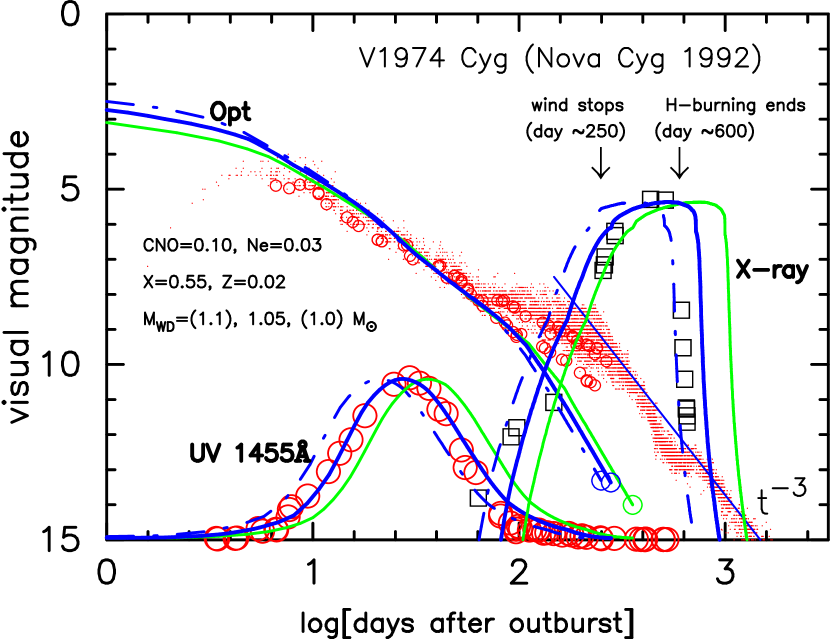
Figure 19.— Calculated free-free emission, UV 1455 Å, and supersoft X-ray light curves are plotted for the best-fit $1.05~{}M_{\sun}$ (thick solid line) WD model together with the $1.0~{}M_{\sun}$ (medium thickness solid line) and $1.1~{}M_{\sun}$ (dash-dotted line) WD models. Fittings of the supersoft X-ray flux (or count rate) and of the UV 1455 Å  flux are shown in Figs. 20 and 21, separately. We assume a chemical composition of $X=0.55$, $X_{\rm CNO}=0.10$, $X_{\rm Ne}=0.03$, and $Z=0.02$ (case Ne 2 in Table 2). The visual observations (small dots) are taken from AAVSO. The $V$ magnitudes (small open circle) are from Chochol et al. (1993). The supersoft X-ray data (open squares) are from Krautter et al. (1996). The UV 1455 Å  data (large open circles) are from Cassatella et al. (2002). Two epochs, which are observationally suggested, are indicated by large upward arrows: one is the epoch when the optically thick winds stop and the other is the epoch when the hydrogen shell-burning ends.

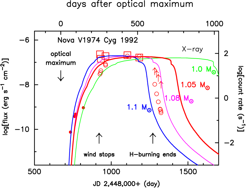
Figure 20.— Calculated X-ray fluxes ($0.1-2.4$ keV) are plotted against time for various WD masses together with the ROSAT observation count rates (open and filled circles: taken from Krautter et al., 1996). Open circles: dominated by soft X-rays. Small filled circles: dominated by hard X-rays. Open squares and small upward arrows: corrected X-ray fluxes and lower limits (Balman et al., 1998). The epoch of the optical maximum corresponds to JD 2,448,673.67, which is 2.67 days after the outburst. Thin solid lines: $1.0$, $1.08$ and $1.1~{}M_{\sun}$ WDs with the envelope composition of $X=0.55$, $X_{\rm CNO}=0.10$, $X_{\rm Ne}=0.03$, and $Z=0.02$ (case Ne 2 in Table 2). Thick solid line: the best-fit model of $1.05~{}M_{\sun}$ WD. Same two epochs as in Fig. 19 are indicated by arrows.

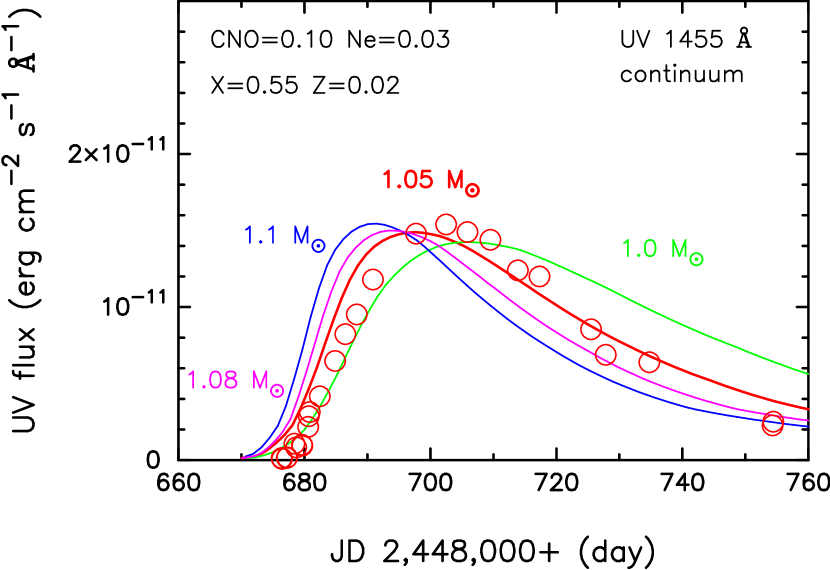
Figure 21.— UV 1455 Å  light curves for the best-fit $1.05~{}M_{\sun}$ (thick solid line) WD model together with the $1.0$, $1.08$ and $1.1~{}M_{\sun}$ (thin solid lines) WD models. We assume a chemical composition of $X=0.55$, $X_{\rm CNO}=0.10$, $X_{\rm Ne}=0.03$, and $Z=0.02$ (case Ne 2 in Table 2). The UV 1455 Å  data (large open circles) are taken from Cassatella et al. (2002). Essentially the same as Fig. 19 except that the abscissa is not logarithmic but linear.

For a fixed abundance of the nova envelope, the only free parameter is the WD mass. We have calculated supersoft X-ray light curves for a wavelength window of $0.1-2.4$ keV with the blackbody model. The best-fit one is obtained for the WD mass of $1.05~{}M_{\sun}$ among 1.0, 1.05, and $1.1~{}M_{\sun}$ as shown in Figures 19 and 20. The supersoft X-ray emerged on day $\sim 260$ after the outburst and remained almost constant during the next $\sim 300$ days, and then decayed rapidly on day $\sim 600$. The $1.05~{}M_{\sun}$ WD model shows a bit longer duration of its supersoft X-ray phase compared with the observation (see also Table 6).

Our calculated X-ray fluxes in Figure 20 show that the more massive the WD, the shorter the duration of the supersoft X-ray phase. This is because a stronger gravity in a more massive WD results in a smaller ignition mass. As a result, hydrogen is exhausted in a shorter period (see, e.g., Kato, 1997, for X-ray turnoff time). Therefore we have calculated X-ray and UV light curves for a $1.08~{}M_{\sun}$ WD, which is between the $1.05$ and $1.1~{}M_{\sun}$ WDs. Fitting becomes much better in the supersoft X-ray but worse in the UV as easily seen from Figure 21. Therefore, we regard the $1.05~{}M_{\sun}$ WD model as the best-fit one at least for the assumed chemical composition.

Comparing our best-fit UV 1455 Å  model with the observation (Cassatella et al., 2002) we obtain a distance of 1.7 kpc. Here we again adopt the absorption law given by Seaton (1979), $A_{\lambda}=8.3E(B-V)=2.65$, together with an extinction of $E(B-V)=0.32$ estimated by Chochol et al. (1997).

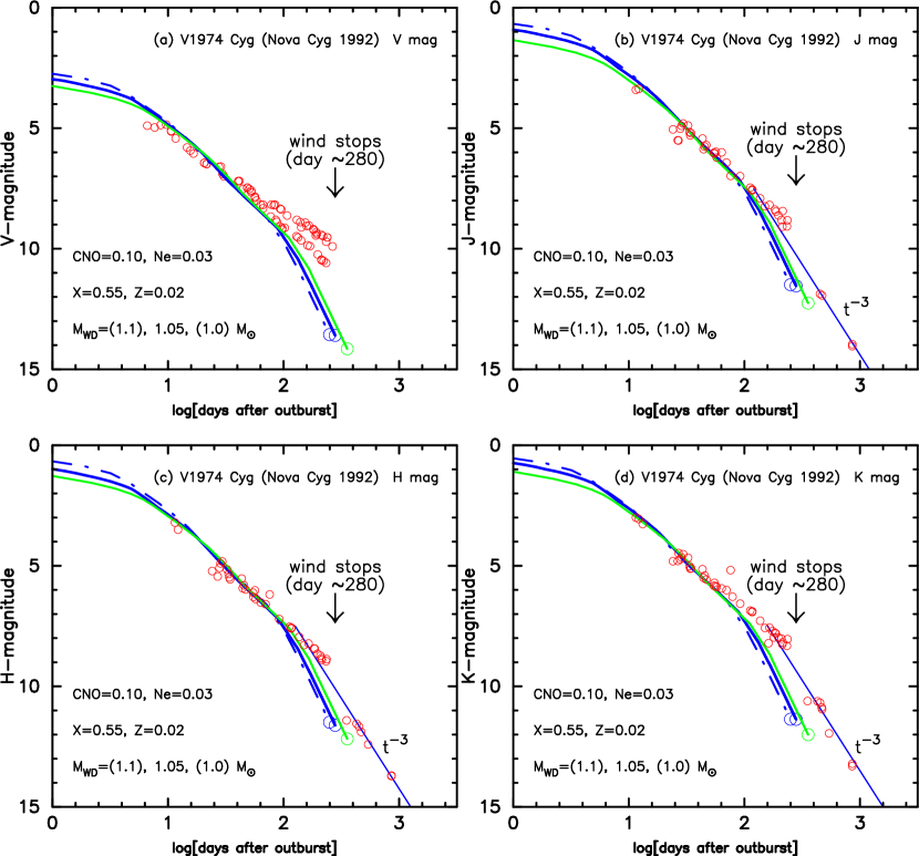
Figure 22.— Calculated free-free emission light curves for the best-fit $1.05~{}M_{\sun}$ (thick solid line) WD model together with the $1.1~{}M_{\sun}$ (dash-dotted) and $1.0~{}M_{\sun}$ (medium thickness solid) WD models. We assume a chemical composition of $X=0.55$, $X_{\rm CNO}=0.10$, $X_{\rm Ne}=0.03$, and $Z=0.02$ (case Ne 2 in Table 2). Each panel shows $(a)$ $V$ magnitude (open circles) taken from Chochol et al. (1993), $(b)$ $J$, $(c)$ $H$, and $(d)$ $K$ magnitudes, IR data (open circles) of which are taken from Woodward et al. (1997). One epoch is indicated by an arrow, i.e.,when the optically thick winds stop for the $1.05~{}M_{\sun}$ WD model. Large open circles at the lower end of each free-free light curve indicate the epoch when the optically thick winds stop. A straight line of $F_{\lambda}\propto t^{-3}$ is also added after the optically thick wind stops.

5.2. Free-free light curves for optical and infrared

We then examine the $V$, $J$, $H$, and $K$ light curves. Figures 19 and 22a show the three different $V$ magnitude observations. Two of them clearly depart from each other after day $\sim 80$. Chochol et al. (1993) explained that this systematic difference in $V$ magnitude comes from the [O III] emission lines locating at the shorter edge of the $V$ bandpass. A different instrumental system with a slightly different $V$ bandpass allows variation of the $V$-magnitude. At the end of 1992 April (day $\sim 75$) strong [O III] 4958.9 and 5006.9 Å  emission lines appeared and the $V$ brightness slightly rose, creating a small bump in the light curve. The discrepancy is more prominent in the visual light curve among observers in Figure 19 (small dot: taken from AAVSO). We find no $y$ magnitude observations of this object. Therefore, we here adopt the faintest one among various $V$ magnitude data for the light curve fitting. Figure 19 shows that our free-free light curve follows the $V$ magnitudes until day $\sim 80$ and it begins to deviate after that.

We have also fitted the $J$ ($1.25\mu$m), $H$ ($1.6\mu$m), and $K$ ($2.3\mu$m) magnitudes in Figure 22 using the same models as in Figure 19. The $J$, $H$, and $K$ data are taken from Woodward et al. (1997), where they summarized their IR observations and concluded that the $V$, $J$, $H$, and $K$ light curves all showed an abrupt transition from a $F_{\lambda}\propto t^{-1.5}$ slope to a $F_{\lambda}\propto t^{-3}$ slope at day $\sim 170$. Our free-free light curve well reproduces these observations until day $\sim 80-100$ and deviates after that.

We have obtained the fitting constants in equation (11), which are $c_{V}=3.73$, $c_{J}=1.68$, $c_{H}=1.75$, and $c_{K}=1.50$, as already shown in Figure 5.

5.3. Distance to V1974 Cyg

Chochol et al. (1997) extensively discussed the distance to V1974 Cyg (catalog ) mainly based on the maximum magnitude versus rate of decline (MMRD) relations and concluded that the most probable value is 1.8 kpc.

Hachisu & Kato (2005) derived a distance of $d=1.7$ kpc from a direct fit with the model UV 1455 Å  light curve. For a distance of $1.7-1.8$ kpc, the peak luminosity is super-Eddington by $\sim 1.8$ mag. Kato & Hachisu (2005) proposed a mechanism of the super-Eddington luminosity and calculated a super-Eddington light curve for V1974 Cyg (catalog ). From the fit with the UV 1455 Å  model they obtain a distance of $1.8$ kpc and a 1.7 mag super-Eddington luminosity. Their distance is a bit larger than the previous result by Hachisu & Kato (2005), because the model UV luminosity increases due to the super-Eddington effect.

In this paper, we adopt a distance of $d=1.8$ kpc, a color excess of $E(B-V)=0.32$, and the same absorption laws as in V1500 Cyg (catalog ).

5.4. Dependence on the chemical composition

Figures 23 and 24 show light curve fittings for another set of the chemical composition (case Ne 1 in Table 2), which is close to the composition obtained by Hayward et al. (1996) as shown in Table 1. We obtain the best-fit $0.95~{}M_{\sun}$ WD model among $1.0$, $0.95$, and $0.9~{}M_{\sun}$ WDs. In this $0.95~{}M_{\sun}$ WD model, $t_{\rm wind}=269$ days and $t_{\rm H-burning}=594$ days. The direct fit with our UV 1455 Å  model indicates a distance of 1.6 kpc.

Sala & Hernanz (2005) calculated static sequences of hydrogen shell-burning and compared the evolutional speed of post-wind phase for V1974 Cyg (catalog ). They suggested that the WD mass is $0.9~{}M_{\sun}$ for 50% mixing of a solar composition envelope with an O-Ne degenerate core (i.e., $X=0.35$, $X_{\rm CNO}=0.25$, and $X_{\rm Ne}=0.16$), or $1.0~{}M_{\sun}$ for 25% mixing (i.e., $X=0.53$, $X_{\rm CNO}=0.13$, and $X_{\rm Ne}=0.08$). Their two cases resemble our models of case Ne 1 and case Ne 2 in Table 2, respectively. Their WD masses are roughly consistent with our values.

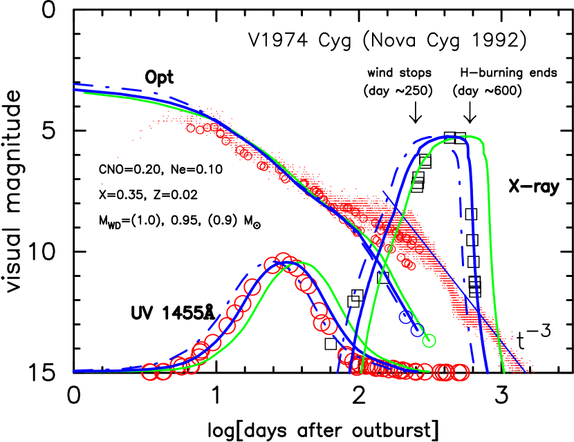
Figure 23.— Same as Fig.19 but for a different chemical composition of $X=0.35$, $X_{\rm CNO}=0.20$, $X_{\rm Ne}=0.10$, and $Z=0.02$ (case Ne 1 in Table 2). The best-fit model is the $0.95~{}M_{\sun}$ WD among the three $0.9$, $0.95$, and $1.0~{}M_{\sun}$ WDs.

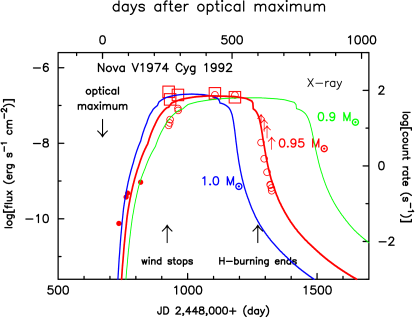
Figure 24.— Same as Fig.20 but for a different chemical composition of $X=0.35$, $X_{\rm CNO}=0.20$, $X_{\rm Ne}=0.10$, and $Z=0.02$ (case Ne 1 in Table 2). The best-fit model is $0.95~{}M_{\sun}$ WD among the $0.9$, $0.95$, and $1.0~{}M_{\sun}$ WDs.

Several groups estimated the WD mass of V1974 Cyg (catalog ). Retter et al. (1997) obtained a mass range of $M_{\rm WD}=0.75-1.07~{}M_{\sun}$ based on the precessing disk model of superhump phenomenon. A similar range of $0.75-1.1~{}M_{\sun}$ is also obtained by Paresce et al. (1995) from various empirical relations on novae. Both our $1.05$ and $0.95~{}M_{\sun}$ WD models are consistent with these constraints.

5.5. Emergence of companion

V1974 Cyg is a binary system with an orbital period of $P_{\rm orb}=0.0812585$ days (1.95 hr) (e.g., De Young & Schmidt, 1994; Retter et al., 1997). The companion mass is estimated to be $M_{2}=0.15~{}M_{\sun}$ from equation (23). For the $1.05~{}M_{\sun}$ WD model, the separation is $a=0.85~{}R_{\sun}$ and the effective radii of the WD Roche lobe and the secondary Roche lobe are $R_{1}^{*}=0.44~{}R_{\sun}$ and $R_{2}^{*}=0.22~{}R_{\sun}$, respectively. In the $0.95~{}M_{\sun}$ WD model, $a=0.82~{}R_{\sun}$, $R_{1}^{*}=0.44~{}R_{\sun}$, and $R_{2}^{*}=0.19~{}R_{\sun}$. The companion emerges from the WD envelope when the photosphere shrinks to $\sim 0.8~{}R_{\sun}$. This epoch is estimated to be day 95 and day 110 for the WD mass of $1.05~{}M_{\sun}$ (case Ne 2) and $0.95~{}M_{\sun}$ (case Ne 1), respectively.

ROSAT observations show that hard X-ray flux increases on day 70–100 and then decays on day 270–300. This hard component is suggested to have originated in the shock between ejecta (Krautter et al., 1996). Hachisu & Kato (2005) suggested a different idea that these hard X-rays originated from a shock between the optically thick wind and the companion. Before day $\sim 70$, the companion resides deep inside the WD photosphere and we do probably not detect hard X-rays. After the companion emerges, the shock front can be directly observed. Then the increase in the hard X-ray flux may correspond to the appearance of the binary component. The decrease in the hard X-ray flux may be caused by the decay of optically thick winds on day $\sim 270-280$.

Table 11Physical properties of three novae

subject/object	units		V1500 Cyg (catalog ) (catalog )	V1668 Cyg (catalog ) (catalog )	V1974 Cyg (catalog ) (catalog )	V1974 Cyg (catalog ) (catalog )
outburst year	year	…	1975	1978	1992	$\leftarrow$
outburst day	JD	…	2,442,653.0	2,443,759.0	2,448,674.5	$\leftarrow$
nova speed class		…	very fast	fast	fast	$\leftarrow$
$t_{2}$	days	…	2.9	12.2	16	$\leftarrow$
$t_{3}$	days	…	3.6	24.3	42	$\leftarrow$
early osc.		…	no	no	no	$\leftarrow$
transition osc.		…	no	no	no	$\leftarrow$
dust		…	no	thin dust	no	$\leftarrow$
orbital period	hours	…	3.35064	3.32	1.9488	$\leftarrow$
secondary mass	$M_{\sun}$	…	0.29	0.29	0.15	$\leftarrow$
obs. WD mass	$M_{\sun}$	…	$>0.9$	$\cdots$	$0.75-1.1$	$\leftarrow$
$E(B-V)$		…	0.45	0.40	0.32	$\leftarrow$
obs. distance	kpc	…	1.5	$\cdots$	$1.8-1.9$	$\leftarrow$
distance from UV fitting	kpc	…	$\cdots$	3.6	1.7	1.6
$t_{\rm break}$ of $y$-band	day	…	70	86	$\cdots$	$\cdots$
cal. WD mass	$M_{\sun}$	…	1.15	0.95	1.05	0.95
wind phase	days	…	180	280	280	260
H-burning phase	days	…	380	720	720	590
separation	$R_{\sun}$	…	1.28	1.21	0.85	0.82
companion’s emergence	days	…	50	100	95	110
chemical composition		…	Ne 2	CO 3	Ne 2	Ne 1
hydrogen content ($X$)		…	0.55	0.45	0.55	0.35

6. Discussion

6.1. Difference in free-free constant

In a nova explosion theory, the evolution of a nova depends on four parameters, i.e., the WD mass, chemical composition of the envelope, mass accretion rate from the companion star, and thermal condition of the WD before the ignition. Our light-curve model basically follows a nova evolution after the nova envelope settles down in a steady state, i.e., after some time has passed from the optical peak. Therefore, the main parameters that govern the evolution of novae are reduced to two from four, i.e., the WD mass and chemical composition. The other two parameters play an important role in the very early phase but do not affect the evolution solution in the steady-state phase. These two parameters are closely linked with the ignition mass and govern the free-free emission parameter, $C_{\lambda}$ in equation(10), because it is determined by the optically thin ejecta outside the photosphere. This is the reason why $C_{\lambda}$ values are different among novae, and this is a subject of a new project.

6.2. CNO abundance

The CNO abundance is taken as a whole because the individual ratios of C, N, and O do not affect the evolution of novae if the total amount of CNO is unchanged. It is because the energy generation of the CNO cycle depends on the total amount of CNO but hardly on the individual ratios in the steady-state phase of novae. The CNO cycle changes only the relative ratio of each C, N, and O but keeps the total amount of C$+$N$+$O unchanged. Moreover, the Rosseland mean opacity is hardly changed if we choose another set of C, N, and O keeping the total amount of C$+$N$+$O constant. Therefore, the individual ratios of C, N, and O hardly affect the envelope evolution.

We assume that, after the optical peak, the chemical composition is constant throughout the envelope (everywhere) and throughout the nova evolution (everytime). We expect that C or O (or Ne) is dredged up from the WD interior in the very early phase of nova outbursts and then mixed into the entire envelope by convection (e.g. Prialnik, 1986). Our assumption means that the convection descends quickly after the optical peak and that the envelope becomes radiative in the decay phase of novae, in which the processed helium concentrates under the hydrogen-burning zone.

From the computational point of view, we have some restrictions in the chemical compositions of OPAL opacity. Therefore, we assume the total amount of CNO as a whole set in order to reduce our computer time and have selected several sets of chemical compositions as shown in table 2.

7. Conclusions

We propose a light curve model based on free-free emission and on the optically thick wind model, and have successfully applied it to three well observed novae, V1500 Cyg (catalog ), V1668 Cyg (catalog ), and V1974 Cyg (catalog ). Our main results are summarized as follows:

(1) We have calculated light curves of novae in which free-free emission from optically thin ejecta dominates the continuum flux. The free-free luminosity is obtained from the density structures outside the photosphere, which are calculated using the optically thick wind model.

(2) The free-free emission light curves are homologous among various white dwarf (WD) masses, chemical compositions, and wavelengths (in optical and infrared). Therefore, we are able to represent a wide range of nova light curves by a single template light curve on the basis of one-parameter family, i.e., a time scaling factor.

(3) The template light curve declines as $F\propto t^{-1.75}$ in the middle part (from $\sim 2$ to $\sim 6$ mag below the optical maximum) and then as $F\propto t^{-3.5}$ in the later part (from $\sim 6$ to $\sim 10$ mag), where $t$ is the time from the outburst in units of days. This break on the light curve is caused by the sharp decrease in the wind mass loss rate. Since the time of the break is proportional to the time scaling factor, we use this time of break to specify the timescale of a nova light curve in the one-parameter family instead of the time scaling factor.

(4) If we know, from observation, the time of break in the light curve, we can tell when the optically thick winds stop (supersoft X-ray turn-on time) and when hydrogen shell-burning ends (supersoft X-ray turnoff time). We can also tell the duration of the ultraviolet (UV) burst phase. These characteristic timescales are uniquely specified by the time of break.

(5) The empirical observational formula between $t_{2}$ and $t_{3}$, i.e., $t_{3}=(1.68\pm 0.08)~{}t_{2}+(1.9\pm 1.5){\rm~{}days}$, is derived from a slope of $F\propto t^{-1.75}$.

(6) Our modeled light curves have been applied to three well-observed novae, V1500 Cyg (catalog ) (Nova Cygni 1975 (catalog )), V1668 Cyg (catalog ) (Nova Cygni 1978 (catalog )), and V1974 Cyg (catalog ) (Nova Cygni 1992 (catalog )). Direct fittings with our free-free light curves indicate the WD mass of $M_{\rm WD}\approx 1.15~{}M_{\sun}$ for V1500 Cyg (catalog ) and $M_{\rm WD}\approx 0.95~{}M_{\sun}$ for V1668 Cyg (catalog ) for the chemical compositions suggested. In V1974 Cyg (catalog ), $M_{\rm WD}\approx 1.05~{}M_{\sun}$ is obtained for the hydrogen content of $X=0.55$ while $M_{\rm WD}\approx 0.95~{}M_{\sun}$ is suggested for the different hydrogen content of $X=0.35$.

(7) Model light curves of the 1455 Å  band nicely follow the observations both for V1668 Cyg (catalog ) and V1974 Cyg (catalog ). Fitting with the UV 1455 Å  light curves, we estimate the distances of V1668 Cyg (catalog ) to be $d=3.6$ kpc for $E(B-V)=0.40$ and the distance of V1974 Cyg (catalog ) to be $d=1.7$ kpc for $E(B-V)=0.32$.

(8) The supersoft X-ray flux was observed in V1974 Cyg (catalog ), which emerged on day $\sim 250$ and declined on day $\sim 600$. This feature is explained consistently by our model. The photospheric temperature rises high enough to emit supersoft X-rays on day $\sim 250-280$, which corresponds to the end of optically thick winds. The X-ray flux keeps a constant peak value for $\sim 300$ days followed by a quick decay on day $\sim 600$, which corresponds to the decay of hydrogen shell-burning.

(9) Finally, we strongly recommend observations with the medium band Strömgren $y$-filter to detect the break of the light curve because the $y$-filter cuts the notorious emission lines in the nebular phase and reasonably follow the continuum flux of novae.

References

- Allen (1981) Allen, C. W. 1981, Astrophysical Quantities (3rd ed.; London: Athlone), 103
- Ando & Yamashita (1976) Ando, H., & Yamashita, Y. 1976, PASJ, 28, 171
- Andreae & Drechsel (1990) Andreae, J., & Drechsel, H. 1990, Physics of Classical Novae, eds. A. Cassatella and R. Viotti (Berin: Springer-Verlag), 204
- Andreä et al. (1994) Andreä, J., Drechsel, H., & Starrfield, S. 1994, A&A, 291, 869
- Arkhipova & Zaitseva (1976) Arkhipova, V. P., & Zaitseva, G. V. 1976, Soviet Astron. Lett., 2, 35
- Arkhipova et al. (2000) Arkhipova, V. P., Burlak, M. A., & Esipov, V. F. 2000, Astronomy Letters, 26, 372
- Augusto & Diaz (2003) Augusto, A., & Diaz, M. P. 2003, AJ, 125, 3349
- Austin et al. (1996) Austin, S. J., Wagner, R. M., Starrfield, S., Shore, S. N., Sonneborn, G., & Bertram, R. 1996, AJ, 111, 869
- Balman et al. (1998) Balman, S., Krautter, J., & Ögelman, H. 1998, ApJ, 499, 395
- Becker & Duerbeck (1980) Becker, H. J., & Duerbeck, H. W. 1980, PASP, 92, 792
- Bode et al. (2006) Bode, M. F. et al. 2006, ApJ, in press (astro-ph/0604618)
- Capaccioli et al. (1990) Capaccioli, M., della Valle, M., D’Onofrio, M., Rosino, L. 1990, ApJ, 360, 63
- Cassatella et al. (2002) Cassatella, A., Altamore, A., & González-Riestra, R. 2002, A&A, 384, 1023
- Cassatella et al. (1979) Cassatella, A., Benvenuti, P., Clavel, J., Heck, A., Penston, M., Macchetto, F., & Selvelli, P. L. 1979, A&A, 74, L18
- Chochol et al. (1997) Chochol, D., Grygar, J., Pribulla, T., Komzik, R., Hric, L., & Elkin, V. 1997, A&A, 318, 908
- Chochol et al. (1993) Chochol, D., Hric, L., Urban, Z., Komzik, R., Grygar, J., & Papousek, J. 1993, A&A, 277, 103
- Cohen (1985) Cohen, J. G. 1985, ApJ, 292, 90
- Collins (1992) Collins, P. 1992, IAU Circ., 5454
- de Freitas Pacheco et al. (1989) de Freitas Pacheco, J. A., dell’Aglio Dias da Costa, R., & Codina, S. J. 1989, ApJ, 347, 483
- De Young & Schmidt (1994) De Young, J. A., & Schmidt, R. E. 1994, ApJ, 431, L47
- Duerbeck et al. (1980) Duerbeck, H. W., Rindermann, R., & Seitter, W. C. 1980, A&A, 81, 157
- Duerbeck & Wolf (1977) Duerbeck, H. W., & Wolf, B. 1977, A&AS, 29, 297
- Ennis et al. (1977) Ennis, D., Becklin, E. E., Beckwith, S., Elias, J., Gatley, I., Matthews, K., Neugebauer, G., & Willner, S. P. 1977, ApJ, 214, 478
- Ferland (1977) Ferland, G. J. 1977, ApJ, 215, 873
- Ferland et al. (1986) Ferland, G. J., Lambert, D. L., & Woodman, J. H. 1986, ApJS, 60, 375
- Ferland & Shields (1978) Ferland, G. J., & Shields, G. A. 1978, ApJ, 226, 172
- Gallagher et al. (1980a) Gallagher, J. S., Hege, E. K., Kopriva, D. A., Butcher, H. R., & Williams, R. E. 1980a, ApJ, 237, 55
- Gallagher et al. (1980b) Gallagher, J. S., Kaler, J. B., Olson, E. C., Hartkopf, W. I., & Hunter, D. A. 1980b, PASP, 92, 46
- Gallagher & Ney (1976) Gallagher, J. S., & Ney, E. P. 1976, ApJ, 204, L35
- Gehrz et al. (1980) Gehrz, R. D., Hackwell, J. A., Grasdalen, G. I., Ney, E. P., Neugebauer, G., & Sellgren, K. 1980, ApJ, 239, 570
- Hachisu & Kato (2000a) Hachisu, I., & Kato, M. 2000a, ApJ, 536, L93
- Hachisu & Kato (2000b) Hachisu, I., & Kato, M. 2000b, ApJ, 540, 447
- Hachisu & Kato (2001a) Hachisu, I., & Kato, M. 2001a, ApJ, 553, L161
- Hachisu & Kato (2001b) Hachisu, I., & Kato, M. 2001b, ApJ, 558, 323
- Hachisu & Kato (2003a) Hachisu, I., & Kato, M. 2003a, ApJ, 588, 1003
- Hachisu & Kato (2003b) Hachisu, I., & Kato, M. 2003b, ApJ, 590, 445
- Hachisu & Kato (2003c) Hachisu, I., & Kato, M. 2003c, ApJ, 598, 527
- Hachisu & Kato (2004) Hachisu, I., & Kato, M. 2004, ApJ, 612, L57
- Hachisu & Kato (2005) Hachisu, I., & Kato, M. 2005, ApJ, 631, 1094
- Hachisu & Kato (2006a) Hachisu, I., & Kato, M. 2006a, ApJ, 642, L53
- Hachisu et al. (2000) Hachisu, I., Kato, M., Kato, T., & Matsumoto, K. 2000, ApJ, 528, L97
- Hachisu et al. (1996) Hachisu, I., Kato, M., & Nomoto, K. 1996, ApJ, 470, L97
- Hachisu et al. (1999a) Hachisu, I., Kato, M., & Nomoto, K. 1999a, ApJ, 522, 487
- Hachisu et al. (1999b) Hachisu, I., Kato, M., Nomoto, K., & Umeda, H. 1999b, ApJ, 519, 314
- Hachisu et al. (2003) Hachisu, I., Kato, M., & Schaefer, B. E. 2003, ApJ, 584, 1008
- Hassall et al. (1990) Hassall, B. J. M., et al. 1990, Physics of Classical Novae, eds. A. Cassatella and R. Viotti (Berin: Springer-Verlag), 202
- Hauschildt et al. (1995) Hauschildt, P. H., Starrfield, S., Shore, S. N., Allard, F., Baron, E. 1995, ApJ, 447, 829
- Hayward et al. (1996) Hayward, T. L., Saizar, P., Gehrz, R. D., Benjamin, R. A., Mason, C. G., Houck, J. R., Miles, J. W., Gull, G. E., & Schoenwald, J. 1996, ApJ, 469, 854
- Horne and Schneider (1989) Horne, K., & Schneider, D. P. 1989, ApJ, 343, 888
- Iglesias & Rogers (1996) Iglesias, C. A., & Rogers, F. J. 1996, ApJ, 464, 943
- Iijima (2006) Iijima, T. 2006, A&A, 451, 563
- Kałużny (1990) Kałużny, J. 1990, MNRAS, 245, 547
- Kato (1983) Kato, M. 1983, PASJ, 35, 507
- Kato (1994) Kato, M. 1994, A&A, 281, L49
- Kato (1997) Kato, M. 1997, ApJS, 113, 121
- Kato (1999) Kato, M. 1999, PASJ, 51, 525
- Kato & Hachisu (1994) Kato, M., & Hachisu, I., 1994, ApJ, 437, 802
- Kato & Hachisu (2005) Kato, M., & Hachisu, I., 2005, ApJ, 633, L117
- Kawara et al. (1976) Kawara, K., Maihara, T., Noguchi, K., Oda, N., Sato, S., Oishi, M., & Iijima, T. 1976, PASJ, 28, no. 1, 1976, p. 163
- Klare et al. (1980) Klare, G., Wolf, B., & Krautter, J. 1980, A&A, 89, 282
- Krautter et al. (1996) Krautter, J., Ögelman, H., Starrfield, S., Wichmann, R., & Pfeffermann, E. 1996, ApJ, .456, 788
- Lance et al. (1988) Lance, C. M., McCall, M. L., & Uomoto, A. K. 1988, ApJS, 66, 151
- Lockwood & Millis (1976) Lockwood, G. W., & Millis, R. L. 1976, PASP, 88, 235
- Lyke et al. (2001) Lyke, J. E. et al. 2001, AJ, 122, 3305
- Lyke et al. (2003) Lyke, J. E. et al. 2003, AJ, 126, 993
- Mallama & Skillman (1979) Mallama, A. D., & Skillman, D. R. 1979, PASP, 91, 99
- Morisset & Péquignot (1996) Morisset, C., & Péquignot, D. 1996, A&A, 312, 135
- Morrison (1978) Morrison, W. 1978, IAU Circ., 3264
- Osborne et al. (2006a) Osborne, J. et al. 2006a, ATel, 764
- Osborne et al. (2006b) Osborne, J. et al. 2006b, ATel, 838
- Orio (2004) Orio, M. 2004, Revista Mexicana de Astronomía y Astrofísica (Serie de Conferencias), Vol. 20. IAU Colloquium 194, pp. 182-186
- Paresce et al. (1995) Paresce, F., Livio, M., Hack, W., & Korista, K. 1995, A&A, 299, 823
- Petitjean et al. (1990) Petitjean, P., Boisson, C., & Pequignot, D. 1990, A&A, 240, 433
- Pfau (1976) Pfau, W. 1976, Inf. Bul. Variable Stars, 1106
- Prialnik (1986) Prialnik, D. 1986, ApJ, 310, 222
- Prialnik & Kovetz (1995) Prialnik, D., & Kovetz, A. 1995, ApJ, 445, 789
- Retter et al. (1997) Retter, A., Leibowitz, E. M., & Ofek, E. O. 1997, MNRAS, 286, 745
- Rieke & Lebofsky (1985) Rieke, G. H., & Lebofsky, M. J. 1985, ApJ, 288, 618
- Saizar et al. (1991) Saizar, P., Starrfield, S., Ferland, G. J., Wagner, R. M., Truran, J. W., Kenyon, S. J., Sparks, W. M., Williams, R. E., & Stryker, L. L. 1991, ApJ, 367, 310
- Saizar et al. (1992) Saizar, P., Starrfield, S., Ferland, G. J., Wagner, R. M., Truran, J. W., Kenyon, S. J., Sparks, W. M., Williams, R. E., & Stryker, L. L. 1992, ApJ, 398, 651
- Saizar et al. (1996) Saizar, P., Pachoulakis, I., Shore, S. N., Starrfield, S., Williams, R. E., Rothschild, E., & Sonneborn, G. 1996, MNRAS, 279, 280
- Sala & Hernanz (2005) Sala, G., & Hernanz, M. 2005, A&A, 439, 1057
- Schmidt (1957) Schmidt, Th. 1957, Z. Astrophys., 41, 181
- Schwarz (2002) Schwarz, G. J. 2002, ApJ, 577, 940
- Schwarz et al. (1997) Schwarz, G. J., Starrfield, S., Shore, S. N., Hauschildt, P. H. 1997, MNRAS, 290, 75
- Scott et al. (1995) Scott, A. D., Duerbeck, H. W., Evans, A., Chen, A.-L., de Martino, D., Hjellming, R., Krautter, J., Laney, D., Parker, Q. A., Rawlings, J. M. C., & Van Winckel, H. 1995, A&A, 296, 439
- Seaton (1979) Seaton, M. J. 1979, MNRAS, 187, 73
- Semeniuk et al. (1995) Semeniuk, I., Olech, A., & Nalezyty, M. 1995, Acta Astron.,
- Shanley et al. (1995) Shanley, L., Ögelman, H., Gallagher, J. S., Orio, M., & Krautter, J. 1995, ApJ, 438, L95
- Shore et al. (2003) Shore, S. N. et al. 2003, AJ, 125, 1507
- Slavin et al. (1995) Slavin, A. J., O’Brien, T. J., Dunlop, J. S. 1995, MNRAS, 276, 353
- Slovak & Vogt (1979) Slovak, M. H. & Vogt, S. S. 1979, Nature, 277, 114
- Snijders et al. (1987) Snijders, M. A. J., Batt, T. J., Roche, P. F., Seaton, M. J., Morton, D. C., Spoelstra, T. A. T., & Blades, J. C. 1987, MNRAS, 228, 329
- Stickland et al. (1981) Stickland, D. J., Penn, C. J., Seaton, M. J., Snijders, M. A. J., & Storey, P. J. 1981, MNRAS, 197, 107
- Tempesti (1979) Tempesti, P. 1979, Astronomische Nachrichten, 300, 51
- Tomkin et al. (1976) Tomkin, J., Lambert, D. L., & Woodman, J. 1976, A&A, 48, 319
- Tylenda (1978) Tylenda, R. 1978, Acta Astron., 28, 333
- Umeda et al. (1999) Umeda, H., Nomoto, K., Yamaoka, H., & Wanajo, S. 1999, ApJ, 513, 861
- Vanlandingham et al. (1997) Vanlandingham, K. M., Starrfield, S., & Shore, S. N. 1997, MNRAS, 290, 87
- Vanlandingham et al. (1999) Vanlandingham, K. M., Starrfield, S., Shore, S. N., Sonneborn, G. 1999, MNRAS, 308, 577
- Vanlandingham et al. (2005) Vanlandingham, K. M., Schwarz, G.J., Shore, S.N., Starrfield, S., & Wagner, R.M. 2005, ApJ, 624, 914
- Wade et al. (1991) Wade, R. A., Ciardullo, R., Jacoby, G. H., & Sharp, N. A. 1991, AJ, 102, 1738
- Warner (1995) Warner, B. 1995, Cataclysmic variable stars, Cambridge, Cambridge University Press
- Williams & Gallagher (1979) Williams, R. E., & Gallagher, J. S. 1979, ApJ, 228, 482
- Williams et al. (1985) Williams, R. E., Ney, E. P., Sparks, W. M., Starrfield, S. G., Wyckoff, S., & Truran, J. W. 1985, MNRAS, 212, 753
- Williams et al. (1978) Williams, R. E., Woolf, N. J., Hege, E. K., Moore, R. L., & Kopriva, D. A. 1978, ApJ, 224, 171
- Woodward et al. (1997) Woodward, C. E., Gehrz, R. D., Jones, T. J., Lawrence, G. F., & Skrutskie, M. F. 1997, ApJ, 477, 817
- Young et al. (1976) Young, P. J., Corwin, H. G., Bryan, J., & de Vaucouleurs, G. 1976, ApJ, 209, 882