Matter density perturbations in interacting quintessence models

Abstract

Models with dark energy decaying into dark matter have been proposed to solve the coincidence problem in cosmology. We study the effect of such coupling in the matter power spectrum. Due to the interaction, the growth of matter density perturbations during the radiation dominated regime is slower compared to non-interacting models with the same ratio of dark matter to dark energy today. This effect introduces a damping on the power spectrum at small scales proportional to the strength of the interaction, $c^{2}$, and similar to the effect generated by ultrarelativistic neutrinos. The interaction also shifts matter–radiation equality to larger scales. We compare the matter power spectrum of interacting quintessence models with the measurments of 2dFGRS. The data are insensitive to values of $c^{2}\leq 10^{-3}$ but strongly constraints larger values. We particularize our study to models that during radiation domination have a constant dark matter to dark energy ratio.

I Introduction

Observations of high redshift supenovae riess , temperature anisotropies of the cosmic background radiation wmap ; wmap3 , matter power spectrum sdss ; 2dgf , and the integrated Sachs–Wolfe signal isw indicate that the Universe is currently undergoing a phase of accelerated expansion reviews . A cosmological constant, $\Lambda$, is frequently invoked as the most natural candidate to drive this acceleration. However, this choice is rather problematic. First, the observed $\Lambda$ value falls by many orders of magnitude below the prediction of quantum field theories weinberg . Second, it is hard to understand why precisely today the vacuum energy density is of the same order of magnitude than that of matter. This remarkable fact, known as the “coincidence problem” coincidence , lacks of a fully convincing theoretical explanation.

Models based on at least two matter components (baryonic and dark) and one dark energy component (with a high negative pressure) have been suggested to explain the accelerated rate of expansion and simultaneously alleviate the coincidence problem peebles_rmph ; dualk . Further, coupling between dark matter (DM) and dark energy (DE) has been suggested as a possible explanation for the coincidence problem amendola ; rong . In particular, the interacting quintessence models of references amendola ; dualk , require the ratio of matter and dark energy densities to be constant at late times. The coupling between matter and quintessence is either motivated by high energy particle physics considerations amendola or is constructed by requiring the final matter to dark energy ratio to be stable against perturbations iqm0 ; iqm ; domainw . The nature of both DM and DE being unknown, there is no physical argument to exclude their interaction. On the contrary, arguments in favor of such interaction have been suggested peebles , and more recently they have been extended to include neutrinos tocchini . As a result of the interaction, the matter density drops with the scale factor $a(t)$ of the Friedmann–Robertson–Walker metric more slowly than $a^{-3}$. The interacting quintessence model studied in the literature have been found to agree with observations of WMAP data and supernovae olivares , but they require values of cosmological parameters different from those of WMAP (first year) concordance model. Observations of the large scale structure can also be used to constrain models. Recent data includes the SDSS sdss and 2dFGRS 2dgf measurements of the matter power spectrum. The analysis of 2dFGRS showed discrepancies with WMAP first year data but is in much closer agreement than SDSS with the results of WMAP third year data wmap .

Currently, there is no compelling evidence for DM–DE interaction szydlowski and its (non-)existence must be decided observationally. It has been suggested that the skewness of the large scale matter distribution is a sensitive parameter to determine the difference in the clustering of baryons and dark matter resulting from the interaction amendola_prl . In this paper we shall study the effect of the interaction on the evolution of matter density perturbations during the radiation dominated period. The evolution of matter and radiation density perturbations provides powerful tools to constrain the physics of the dark sector koivisto . We will show how the shape of the matter power spectrum can be a directly related with the interaction and we will use the matter power spectrum measured by the 2-degree field galaxy redshift survey (2dFGRS, for short) to set constraints on the interaction. The outline of the paper is as follows: In Section II, we present a brief summary of the interacting quintessence model (IQM, hereafter). In Section III we describe the evolution of matter and radiation perturbations in models with dark matter and dark energy. In Section IV we discuss some analytical solutions and in Section V we show how the slope of a scale invariant matter density perturbations has less power on small scales than non-interacting models. In Section VI we describe the results of Monte Carlo Markov chains constructed to compare the model with the observations. Finally, Section VII summarizes our main results and conclusions.

II The interacting quintessence model

Most cosmological models implicitly assume that matter and dark energy interact only gravitationally. In the absence of an underlying symmetry that would suppress a matter – dark energy coupling (or interaction) there is no a priori reason for dismissing it. Cosmological models in which dark energy and matter do not evolve separately but interact with one another were first introduced to justify the small value of the cosmological constant wetterich . Recently, various proposals at the fundamental level, including field Lagrangians, have been advanced to account for the coupling federico . Scalar field Lagrangians coupled to matter generically do not generate scaling solutions with a long enough dark matter dominated period as required by structure formation amendola-challenges . The phenomenological model we will be considering was constructed to account for late acceleration in the framework of Einstein relativity and to significantly alleviate the aforesaid coincidence problem iqm0 ; iqm and escapes the limits imposed by amendola-challenges . Here we shall describe its main features. For further details see Refs. iqm ; dualk ; section2 .

The model considers a spatially flat Friedmann–Robertson–Walker universe filled with radiation, baryons, dark matter (subscript, $c$) and dark energy (subscript, $x$). Its key assumption is that dark matter and dark energy are coupled by a term $Q=3Hc^{2}(\rho_{c}+\rho_{x})$, that gauges the transfer of energy from the dark energy $\rho_{x}$ to the dark matter $\rho_{c}$. The quantity $c^{2}$ is a small dimensionless constant that measures the strength of the interaction, and $H=a^{-1}\,da/dt$ is the Hubble function. To satisfy the severe constraints imposed by local gravity experiments peebles_rmph ; hagiwara , baryons and radiation couple to the other energy components only through gravity. Thus, the energy balance equations for dark matter and dark energy take the form

$$\frac{d\rho_{c}}{dt}+3H\rho_{c}=Q\,,\qquad\frac{d\rho_{x}}{dt}+3H(1+w_{x})\rho_{x}=-Q\,,$$ (1)

where $w_{x}=p_{x}/\rho_{x}<-1/3$ is the equation of state parameter of the dark energy fluid.

Our ansatz for $Q$ guarantees that the ratio between energy densities $r\equiv\rho_{c}/\rho_{x}$ tends to a fixed value at late times. This can be seen by studying the evolution of $r$ which is governed by

$$\frac{dr}{dt}=-3\Gamma Hr\,,\quad\qquad\Gamma=-w_{x}-c^{2}\frac{(\rho_{c}+\rho_{x})^{2}}{\rho_{c}\,\rho_{x}}\,.$$ (2)

The stationary solutions of Eq. (2) follow from solving $r_{s}\,\Gamma(r_{s})=0$. When $w_{x}$ is a constant these solutions are given by the roots of the quadratic expression

$$r^{\pm}_{s}=-1+2b\pm 2\sqrt{b(b-1)}\,,\qquad b=-\frac{w_{x}}{4c^{2}}>1.$$ (3)

As it can be checked by slightly perturbing Eq. (2), the stationary $r^{+}_{s}$ solution is unstable while $r^{-}_{s}$ is stable. The general solution of Eq. (2) can be written as

$$r(x)=\frac{r^{-}_{s}+xr^{+}_{s}}{1+x}\,,$$ (4)

where $x=(a/a_{0})^{-\lambda}$ with $\lambda\equiv 12\,c^{2}\sqrt{b(b-1)}$. In the range $r^{-}_{s}<r<r^{+}_{s}$ $r(x)$ is a monotonic decreasing function. Thus, as the Universe expands, $r(x)$ gently evolves from $r_{s}^{+}$ to the attractor solution $r^{-}_{s}$. The transition from one asymptotic solution to the other occurs only recently (see Fig. 2 of olivares ) so we can take $r\simeq r^{+}_{s}$ during a fairly large part of the history of the Universe. Finally, the constraint on $r_{s}^{+}\simeq$ const implies that $r$ and $c^{2}$ are not independent, but linked by $c^{2}(r_{s}^{+}\,+1)^{2}=r_{s}^{+}\,\mid w_{x}\mid$, so the product $c^{2}r_{s}^{+}\sim\mid w_{x}\mid$ is of order unity.

We would like to remark that the above ansatz for $Q$ is not arbitrary. It was chosen so that the ratio between dark matter and dark energy densities tends to a fixed value at late times, thereby alleviating the coincidence problem iqm ; dualk ; section2 . It also yields a constant but unstable ratio at early times. It is hard to imagine a simpler expression for $Q$ entailing these two key properties. Likewise, it is only fair to acknowledge that the aforesaid expression can be re–interpreted as implying, at late times, an effective exponential potential for the quintessence field. This well–known result was derived by Zimdahl et al. iqm0 . Likewise, in olivares we remarked that the effective potential of the IQM model exhibits a power–law dependence on the quintessence field at early times and an exponential dependence at late times.

Near $r\approx r^{-}_{s}$ the balance Eqs. (1) can be approximated by

$$\frac{1}{\rho_{c}}\,\frac{d\rho_{c}}{dr} \simeq \frac{1-c^{2}(1+1/r^{-}_{s})}{c^{2}(r^{+}_{s}-r^{-}_{s})(r-r^{-}_{s})}\,,$$

$$\frac{1}{\rho_{x}}\,\frac{d\rho_{x}}{dr} \simeq \frac{1+w_{x}+c^{2}(1+r^{-}_{s}}{c^{2}(r^{+}_{s}-r^{-}_{s})(r-r^{-}_{s})}\,\,.$$ (5)

For $w_{x}\simeq$ constant, these equations can be integrated to

$$\rho_{c}\propto a^{-3\left[1-c^{2}(1+1/r^{-}_{s})\right]}\,,\qquad\rho_{x}\propto a^{-3\left[1+w_{x}+c^{2}(1+r^{-}_{s})\right]}\,.$$ (6)

Notice that the condition $\Gamma(r^{-}_{s})=0$ implies that the exponents in the energy densities, Eq. (6), coincide. Interestingly, these results are not only valid when the dark energy is a quintessence field (i.e., $-1<w_{x}<-1/3$), they also apply when the dark energy is of phantom type (i.e., $w_{x}<-1$), either a scalar field with the “wrong sign” for the kinetic energy term, a k-essence field, or a tachyon field dualk .

Near the attractor, dark matter and dark energy dominate the expansion and Friedmann equation becomes simply $3\,H^{2}=\kappa(\rho_{c}+\rho_{x})$ and $a\propto t^{(2/3)[1+w_{x}+c^{2}(1+r^{-}_{s})]^{-1}}$. The results presented here significantly alleviates the coincidence problem but they do not solve it in full. For this purpose, one needs to show that the attractor was reached only recently -or that we are very close to it- and that $r^{-}_{s}$ is of order unity. In fact, the value of $r^{-}_{s}$ cannot be derived from data and must be understood as an input parameter. This is also the case of a handful of key cosmic quantities such as the current value of the cosmic background temperature, the Hubble constant or the ratio between the number of baryons and photons.

III Linear perturbations

As the scalar field is coupled just to dark matter and since dark matter and quintessence are coupled to baryons and photons only gravitationally, there is no transfer of energy or momentum from the scalar field to baryons or radiation and their evolution is the same as in non-interacting models. In the synchronous gauge and for a flat space-time, the line element is given by: $ds^{2}=a^{2}(\tau)[-d\tau^{2}+(\delta_{K,ij}+h_{ij})dx^{i}dx^{j}]$, where $\tau$ is the conformal time, $a$ the scale factor and $\delta_{K,ij}$ is Kronecker’s delta tensor. Only two functions $h$ and $\mu$ are necessary to characterize the scalar mode of the metric perturbations $h_{ij}$ bertschinger . Assuming the dark energy energy-momentum tensor is free of anisotropic stresses, the equations describing the dark matter and dark energy evolution in the synchronous gauge are:

$$\dot{\delta_{x}} = -(1+w_{x})(\theta_{x}+\frac{\dot{h}}{2})-3{\mathcal{H}}(1-w_{x})\delta_{x}-9{\mathcal{H}}^{2}(1-w_{x}^{2})\frac{\theta_{x}}{k^{2}}+3{{\mathcal{H}}}c^{2}(\delta_{x}+r\delta_{c})\,,$$ (7)

$$\dot{\theta_{x}} = 2{{\mathcal{H}}}\theta_{x}+\frac{k^{2}}{1+w_{x}}\delta_{x}-3{{\mathcal{H}}}\frac{c^{2}}{1+w_{x}}(1+r)\theta_{x},$$ (8)

$$\dot{\delta_{c}} = -\theta_{c}-\frac{\dot{h}}{2}-3{{\mathcal{H}}}c^{2}(\delta_{c}+\frac{\delta_{x}}{r})\,,$$ (9)

$$\dot{\theta_{c}} = -{{\mathcal{H}}}\theta_{c}+3{{\mathcal{H}}}c^{2}(1+1/r)\theta_{x}.$$ (10)

In these expressions, the derivatives are taken with respect to the conformal time $\tau$, $\delta$ is the density fluctuation, $\theta$ the divergence of the fluid velocity, $h$ the gravitational potential, $k$ the wavenumber of a Fourier mode, ${{\mathcal{H}}}=\dot{a}/a$ and, $r$ is the ratio of the background cold dark matter to the dark energy density. We also assume that the dark energy has constant equation of state parameter $w_{x}=$ constant and sound speed $c_{s,x}=1$. In this gauge, $(\delta P/\delta\rho)_{x}\delta_{x}=c^{2}_{s,x}\delta_{x}+3{\mathcal{H}}\theta_{x}(1+w_{x})(c^{2}_{s,x}-w_{x})/k^{2}$. As noted in koivisto , Eq. (10) was mistyped in olivares .

Equations (7)–(10) do not form a closed set. They must be supplemented with the equations describing the evolution of the coupled baryon–photon fluid, neutrinos and gravitational potentials. For the potentials, the only relevant quantity is the trace of the metric perturbation, $h$. Its time evolution can be derived from Einstein’s equations:

$$\ddot{h}+{{\mathcal{H}}}\dot{h}=-3{{\mathcal{H}}}^{2}\sum_{i}\left(1+3\,(\delta P/\delta\rho)_{s,i}^{2}\right)\delta_{i}\Omega_{i}\,,$$ (11)

where the sum is over all matter fluids and scalar fields; $\Omega_{i}$ is the energy density of fluid $i$ in units of the critical density. With respect to baryons, photons and neutrinos, they interact with the DM and DE only through gravity.

The coupled evolution of dark matter, dark energy, baryon, photon and, optionally, neutrino density perturbations and gravitational fields can not be solved analytically. To compute numerically the solution, we have implemented Eqs. (7)–(11) into the CMBFAST code cmbfast . In Fig. 1 we show the evolution of the potential, $h$, and the matter density perturbation, $\delta_{c}$, for three modes of wavelength $k=0.01,0.1$ and $1h$ Mpc^-1 and for three different values of the DE decay rate: $c^{2}=0$ (solid line), $c^{2}=10^{-3}$ (dotted line) and $c^{2}=6\times 10^{-3}$ (dashed line). In all the cases, the cosmological parameters defining the background model are: $\Omega_{c}=0.26$, $\Omega_{b}=0.04$, $\Omega_{x}=0.7$, $w_{x}=-0.9$ and the Hubble constant $H_{0}=70$ km/s  Mpc^-1.

Figure 1: Evolution of the gravitational potential (upper panels) and the cold dark matter density perturbations (lower panels) for three modes: $k=0.01$ (left) $k=0.1$ (center) and $k=1h^{-1}$Mpc (right panels). We study the evolution of each mode in three different cosmological models: the concordance model ($c^{2}=0$, solid line) and two interacting quintessence models with the same cosmological parameters, $c^{2}=10^{-3}$ (dotted) and $c^{2}=6\times 10^{-3}$ (dashed line).

As panels 1e and 1f illustrate, modes that enter the horizon before matter-radiation equality grow slower with increasing interaction rate. As a result, the matter power spectrum on those scales will have less power than in non-interacting models. To obtain some insight on the behavior on the evolution of matter density perturbations, we will be considering some limiting cases where analytic solutions exist. For simplicity, we shall assume the dynamical effect of baryons and neutrinos in the evolution of dark matter and dark energy density perturbations can be neglected. The result of combining Eqs. (9) and (10), considering only the leading terms at first order in the interaction $c^{2}$, is

$$\ddot{\delta}_{c}+{\mathcal{H}}(1+3c^{2})\dot{\delta}_{c}+3c^{2}{\mathcal{H}}^{2}\left(\frac{1-3w_{B}}{2}+\frac{3c^{2}(r+1)}{(1+w_{x})A}\right)\delta_{c}=-{1\over 2}(\ddot{h}+{\mathcal{H}}\dot{h})+c^{2}F(\dot{\delta}_{x},\delta_{x}),$$ (12)

with

$$F(\dot{\delta}_{x},\delta_{x}) = 3{\mathcal{H}}\dot{\delta}_{x}+3\frac{{\mathcal{H}}^{2}}{r}\left[\frac{3(r+1)(1-w_{x}-c^{2})}{(1+w_{x})A}-\frac{1-3w_{B}}{2}\right]\delta_{x}\,,$$ (13)

$$A = 1+(3{\mathcal{H}}/k)^{2}(1-w_{x}^{2})\,.$$ (14)

Equation (12) corresponds to a damped harmonic oscillator (with real or imaginary frequencies) with a forcing term that, since $c^{2}\ll 1$, is dominated by the time evolution of the gravitational potential. In this approximation, Eq. (11) gives

$$\ddot{\delta}_{c}+{\mathcal{H}}(1+3c^{2})\dot{\delta}_{c}-3{\mathcal{H}}^{2}\left[\frac{\Omega_{c}}{2}\left(1+{3(1-w_{x})(3{\mathcal{H}}/k)^{2}\over A}c^{2}\right)-c^{2}\left(\frac{3c^{2}(r+1)}{(1+w_{x})A}+\frac{1-3w_{B}}{2}\right)\right]\delta_{c}=3{\mathcal{H}}^{2}(\Omega_{\gamma}\delta_{\gamma}+2\Omega_{x}\delta_{x})\,.$$ (15)

In the limit $c^{2}=0$ this equation coincides with the evolution of matter density perturbation in non-interacting cosmologies. The effect of the interaction is to increase the friction term and to modify the oscillation frequency. The term in square brackets accounts for the self attractive force acting on the perturbation; the extra contribution arises due to the interaction. The effect of the DM–DE coupling can be understood as a modification of the effective gravitational constant. This result was previously found in amendola2004 and corasaniti , both models with a different interaction ansatz. In our case, the interaction provides a new physical effect not present in other models: if $w_{x}\sim-1$, the second term in the square parenthesis could dominate and matter density perturbations would stop growing and start oscillating.

IV Evolution of matter density perturbations

IV.1 Superhorizon sized perturbations

The time variation of dark matter and dark energy densities have analytic expressions in terms of the expansion factor (Eq. (6)). In terms of the time variable $\log a$, analytic solutions can be found for the evolution of superhorizon sized perturbations. Using this new time variable Eq. (15) can be written as

$$\delta_{c}^{\prime\prime}+\left(\frac{1-3w_{B}}{2}+3c^{2}\right)\delta_{c}^{\prime}+3c^{2}\left(\frac{1-3\omega_{B}}{2}\right)\delta_{c}=\frac{3}{2}(1+3c^{2}_{s,B})\frac{\delta\rho_{B}}{\rho_{B}}\,,$$ (16)

where prime denotes derivatives with respect to $\log a$. The subindex $B$ stands for background quantities. The behavior of $\delta\rho_{B}/\rho_{B}$ at scales larger than the Jean’s length can be parameterized as:

$$\frac{\delta\rho_{B}}{\rho_{B}}=\left(\frac{\delta\rho_{B}}{\rho_{B}}\right)_{H_{I}}\left(\frac{a}{a_{H_{I}}}\right)^{p/2}\,,$$ (17)

where $(\delta\rho_{B}\rho_{B})_{H_{I}}$ is the amplitude of the mode under consideration at horizon crossing, at time $a_{H_{I}}$. After a brief transient period, the evolution of the dark matter and dark energy perturbations will be given by the inhomogeneous solution associated with the time evolution of the gravitational potential: $\delta_{c}\sim h\sim a^{p/2}$. The solutions of eq (16) are: $p=(4;\;2-6.6c^{2})$ in the radiation and cold dark matter dominated periods, respectively. For non-interacting models, the well known solutions are $p=(4;\;2)$. These solutions were to be expected; as discussed in padma , if $\rho_{c}\sim a^{-\alpha}$, being $\alpha$ a constant, then $p\simeq 2(\alpha-2)$. In the radiation epoch, $\alpha=4$, and in the matter epoch $\alpha=3(1-c^{2})$. Thus, during matter domination, the growth of dark matter density perturbations slows down with respect to those of non-interacting models but, in general, the evolution of superhorizon sized perturbations is not significantly altered by the interaction.

IV.2 Subhorizon sized matter perturbations

For perturbations inside the horizon, Eqs. (7) and (8) have the approximate solution,

$$\delta_{x}=3\left({{\mathcal{H}}\over k}\right)^{2}c^{2}r\delta_{c}\,.$$ (18)

Since $c^{2}\ll 1$, we have that $\Omega_{c}\delta_{c}\gg\Omega_{x}\delta_{x}$ and the force term in Eq. (15) is dominated by the perturbations in the photons field during the radiation epoch. In the small scale limit ($3{\mathcal{H}}/k\ll 1$), $A\simeq 1$ and

$$\ddot{\delta}_{c}+{\mathcal{H}}(1+3c^{2})\dot{\delta}_{c}-4\pi Ga^{2}\rho_{c}\left[1+\frac{3c^{2}rw_{x}}{4\pi G\rho_{c}a^{2}(r+1)(1+w_{x})}\right]\delta_{c}={3\over 2}{\mathcal{H}}^{2}\Omega_{\gamma}\delta_{\gamma}.$$ (19)

Even this simplified equation does not have simple analytic solutions. The slower growth of matter density perturbations in the IQM compared with non–interacting ones can be understood analyzing the different coefficients: (A) the interaction increases the friction term, damping more rapidly the homogeneous solution and (B) it decreases the gravitational force acting on the perturbation. At very early times, when $\Omega_{c}\leq 6c^{2}\mid w_{x}/(1+w_{x})\mid$, and well within the horizon perturbations on the photon field oscillate and matter perturbations do not grow but undergo damped oscillations peeb_ratra . The characteristic time–scale of the growth of matter density perturbations is the mean free–fall time, $t_{ff}\sim(G\rho_{c})^{-1/2}$. During the radiation dominated regime the expansion rate is fixed by Friedmann equation: $H\sim\sqrt{G\rho_{\gamma}}$ and since $t_{ff}>>H^{-1}$, perturbations only grow logarithmically, not as a power law. In our IQM this effect is more severe. First, at all times the matter density is smaller than in non–interacting models but with the same values for the cosmological parameters today. Second, the effective gravitational force is reduced. Thus, the mean free–fall time increases and density perturbations grow slower (or get even erased), compared with a non–interacting model.

Scalar fields coupled to matter would modify gravity inducing an extra attractive force. A repulsive effect could be obtained by the exchange of vector bosons. It was first suggested amendola-phantom that phantom scalar fields with non-standard kinetic term coupled to matter would give rise to a long-range repulsive force. In our phenomenological model, the decrease of the gravitational coupling in Eq. (19) is due to our specific ansatz $Q$ for the dark matter – dark energy interaction.

IV.3 Comparison with other interacting models

Interacting quintessence models couple dark matter and dark energy so the energy momentum tensor of the DM and DE are not separately conserved but obey $(T^{\mu}_{(\phi)\nu}+T^{\mu}_{(c)\nu})_{;\mu}=0$. In references amendola ; amendola2004 the coupling is chosen such that $\dot{\rho_{c}}+3{\mathcal{H}}\rho_{c}=(16\pi G/3)^{1/2}\,\beta\rho_{c}\dot{\phi}_{x}$, where $\phi_{x}$ is the scalar field describing the dark energy component and $\beta$ the decay rate coefficient whom, in general, is a time varying function. By assuming that the scalar field couples to dark matter only, the evolution of matter density perturbations in the synchronous gauge is given by

$$\dot{\delta}_{c} = -\theta_{c}-{1\over 2}\dot{h}-\frac{d}{d\tau}(\beta\varphi)\,,$$ (20)

$$\dot{\theta}_{c} = -{\mathcal{H}}(1-2\beta x)\theta_{c}-2\beta k^{2}\phi\,.$$ (21)

In this expression, $\varphi=(4\pi G/3)^{1/2}\delta\phi_{x}$ is the perturbation in the scalar field and $x$ its kinetic energy. The evolution of the gravitational field does not depend on the specific interaction ansatz, and is given by Eq. (11). For subhorizon sized perturbations, $\varphi=k^{-2}{\mathcal{H}}(\beta\Omega_{c}\delta_{c})$ and, in the radiation dominated regime, matter perturbations evolve as

$$\ddot{\delta}_{c}+{\mathcal{H}}[1-2\beta x]\dot{\delta}_{c}-4\pi Ga^{2}[1+{4\over 3}\beta^{2}]\rho_{c}\delta_{c}={3\over 2}{\mathcal{H}}^{2}2\Omega_{\gamma}\delta_{\gamma}\,.\$$ (22)

As discussed above, during the radiation period the background expansion rate is fixed by Friedmann’s equation, but the mean free–fall time is now: $t_{ff}\sim[G(1+4\beta^{2}/3)\rho_{c}]^{1/2}$. Due to the interaction, the dark matter density at any given time is smaller than in a non-interacting model with the same cosmological parameters, and the difference increases with $\beta$. Likewise, the effective gravitational constant increases, but since the dependence is second order in $\beta$, one would expect $t_{ff}$ to be smaller than in non-interacting models. This statement depends on the particular interaction ansatz. Since perturbations evolve as if the Newton’s gravitational constant was a factor $(1+4\beta^{2}/3)$ larger, the interaction with the scalar field could make density perturbations to grow faster during the matter dominated regime due to a larger local gravity. This effect could compensate the slow growth during the radiation dominated regime and enhancing the clustering of dark matter perturbations compared with the uncoupled case, as found in corasaniti . But even in this case, the amplitude of the matter power spectrum was smaller in the range $(0.01-0.4)h$ Mpc^-1.

V The effect of the Interaction on the Matter Power Spectrum

In the previous section we have shown that the interaction slows the growth of matter density perturbations. Only the slower growth of perturbations in the radiation dominated regime will have a significant impact on the matter power spectrum today. For comparison, we shall assume that in interacting and non-interacting models density perturbations have the same amplitude when they come within the horizon. For non-interacting models, this prescription leads to the so called Harrison–Zeldovich power spectrum harrison-zeldovich , characterized by a functional form $P(k)\sim k^{n_{s}}$ with $n_{s}=1$ on large scales. During the matter epoch, if density perturbations evolve with the scale factor as $\delta_{c}\sim a^{p/2}$ and the background energy density as $\rho_{c}\sim a^{-\alpha}$ (with $\alpha=$const) the power spectrum will scale with wavenumber as

$$P(k)\sim k^{-3+2p/(\alpha-2)}\,.$$ (23)

During the matter dominated period $p\simeq 2(\alpha-2)+0.6c^{2}$ and the slope of a scale-invariant spectrum is $n_{s}=1$, with a very weak dependence on the interaction.

Figure 2: (a) Matter power spectra for the interacting quintessence model with different rates of energy transfer. From top to bottom $c^{2}=0,10^{-3},6\times 10^{-3},10^{-2}$. We took the present value of cosmological parameters to be: $\Omega_{b}=0.04$, $\Omega_{cdm}=0.23$, $H_{0}=72$km s${}^{-1}/$Mpc, $\Omega_{\Lambda}=0.73$ the dark energy equation of state $w_{x}=-0.9$ and the slope of the matter power spectrum at large scales $n_{s}=1$. (b) The same for mixed dark matter models with one single species of massive neutrinos. From top to bottom, the fraction of energy density in the form of neutrinos is: $\Omega_{\nu}=0.01,0.05,0.1,0.2$. As before, the total dark matter energy density was $\Omega_{dm}=0.23$, the rest was cold dark matter. (c) Variation of the slope of $P(k)$ with $c^{2}$, and (d) with massive neutrinos. The slope was computed from a straight line fit to the data in the interval $k=[0.1,1]h^{-1}$ Mpc.

The slope of the matter power spectrum on scales $k\geq k_{eq}$ is determined by the growth rate of subhorizon sized matter perturbations during radiation domination. If a mode that crosses the horizon before matter–radiation equality ($k\geq k_{eq}$) grows as $\delta_{c}\sim\tau^{q/2}$ during the radiation dominated period, then the amplitude of the power spectrum today would be $P(k)=P(k_{eq})(k_{eq}/k)^{-3+q}$. For cold dark matter models, dark matter perturbations experience only a logarithmic growth, so models with less growth will have less power at small scales as do, for example, mixed dark matter models davis , i.e., models containing a significant fraction of massive neutrinos.

In Fig. 2a we plot the power spectrum for different interacting quintessence models. All models have the cosmological parameters of the WMAP first year concordance model wmap . From top to bottom, $c^{2}=0,10^{-4},10^{-3},10^{-2}$; the normalization is arbitrary. Similarly, in Fig. 2b we plot the matter power spectrum of mixed dark matter models with one species of massive neutrinos, for different neutrino masses: $m_{\nu}=0,0.1,1,10$ eV. With increasing decay rate or neutrino mass, the matter power spectrum shows larger oscillations, due to the increased ratio of baryons to dark matter. The slope decreases with increasing $c^{2}$ and $m_{\nu}$. As explained above, potential wells are shallower with increasing $c^{2}$; matter perturbations during radiation domination are damped similarly as do in models with massive neutrinos. In Fig. 2c we plot the change in the slope of the matter power spectrum as a function of the energy transfer rate and in 2d as a function of the neutrino mass. As the slope changes smoothly from large to small scales, for convenience we computed the slope as a straight line fit to the data in the interval $k=[0.1,1.0]h^{-1}$Mpc. In both cases the behavior is rather similar: for low values of neutrino mass and interaction coupling, the slope is approximately $-2$ and roughly constant. When parameters are increased in either model, the slope decreases. Observations of large scale structure that constrain the neutrino mass can also be used to set constraints on the strength of DM–DE coupling during the radiation dominated period. These constraints are complementary to those coming from skewness of the matter density field, that are sensitive to the interaction at much lower redshifts amendola_prl . Fig. 2 shows a significant difference between massive neutrinos and interacting quintessence: in IQM the maximum of the matter power spectrum shifts to larger scales. At larger $c^{2}$, the dark matter density becomes smaller at any given redshift and the matter radiation equality is delayed. This does not happen in models with massive neutrinos where matter-radiation equality occurs always at the same redshift.

VI Observational Constraints on Dark Matter - Dark Energy coupling

Since the interaction affects the slope of the matter power spectrum, we used the 2dFGRS data 2dgf to constrain $c^{2}$. We used a Monte Carlo Markov chain to run the CMBFAST code, adapted to solve the IQM described above, through a 7-dimensional parameter space: ($A$, $\Omega_{b}h^{2}$, $\Omega_{c}h^{2}$, $H_{0}$, $n_{s}$, $c^{2}$, $w_{x}$) where $A$ is the normalization of the matter power spectrum, $\Omega_{b}$, $\Omega_{c}$ are the baryon and cold dark matter fraction in units of the critical density, $n_{s}$ is the slope of the matter power spectrum at large scales, $c^{2}$ measures the transfer rate of dark energy into dark matter and $w_{x}$ is the dark energy equation of state parameter. Hereafter $H_{0}=100h$ km/s Mpc^-1. It is common practice to call $h$ the Hubble constant in units of $100$km s${}^{-1}/$Mpc and we shall follow this convention. It should not be confused with the gravitational potential in the synchronous gauge introduced in Sec. III. We limit our study to flat models, so the fraction of dark energy is fixed by the Friedmann equation $\Omega_{x}+\Omega_{b}+\Omega_{c}+\Omega_{\gamma}=1$, where $\Omega_{\gamma}$ is the photon energy density, and all densities are measured in units of the critical density. To simplify, we studied only adiabatic initial conditions and initial power spectrum with no running on the spectral index. We did not include reionization, or gravitational waves, since they have little effect on the matter power spectrum.

Since we are interested in constraining $c^{2}$ from the shape of the matter power spectrum, we have to correct for non-linear effects. We followed the 2dFGRS team and assumed the non-linear biasing to be well described by

$$P_{gal}(k)=b^{2}{1+Qk^{2}\over 1+A_{g}k}P_{lin,dm}(k).$$ (24)

We used $A_{g}=1.4$ and $Q=4.6$. We marginalized over the bias factor $b$. We did not use the SDSS galaxy power spectrum because these data were analyzed in real space where non-linear effects are more important. We used the likelihood codes provided by the 2dFGRS team 2dgf . As priors, we imposed our chains to take values within the intervals: $A=[0.5,2.0]$ in units of COBE normalization, $h=[0.4,1.1]$, $\Omega_{b}h^{2}=[0.00,0.05]$, $\Omega_{c}h^{2}=[0.0,0.5]$, $n_{s}=[0.80,1.2]$, $w_{x}=[-0.5,-1.0]$ and $c^{2}=[0,0.05]$. We run the chain for $10^{5}$ models, that were sufficient to reach convergence. In Fig. 3 we plot the marginalized likelihood function obtained from the posterior distribution of models. The likelihood is very non-gaussian, reflecting the fact that models do not depend linearly on $c^{2}$. The data are rather insensitive to $c^{2}\leq 10^{-3}$ since the slope does not change significantly up to that value (see Fig. 2c). As discussed above, increasing the interaction rate leads to smaller fraction of dark matter during the radiation dominated period and shallower potential wells, larger free–fall times and, as a result, the amplitude of the matter power spectrum is damped (see Fig. 1e).

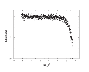
Figure 3: Marginalized likelihood function for the 2dFGRS data.

In Fig. 4 we show the joint confidence contours at the 68%, 95% and 99.99% level for pairs of parameters after marginalizing over the rest. Our prior on the spectral index was too restrictive and did not allow the chains to sample all the parameter space allowed by the data. Therefore, we can not draw definitive conclusions about the confidence intervals for all of the parameters. The figure does show that the data at present do not have enough statistical power to discriminate the IQM from non-interacting ones. Our $1\sigma$ confidence levels and upper limits for the cosmological parameters are $c^{2}\leq 3\times 10^{-3}$, $\Omega_{c}h^{2}=0.1\pm 0.02$, $H_{0}=83^{+6}_{-10}$km s${}^{-1}/$Mpc. The data are rather insensitive to $w_{x}$ and baryon fraction. Models with $c^{2}=0$ are compatible with the 2dFGRS data at the $1\sigma$ level. The data show a full degeneracy with respect to $c^{2}$ up to $c\simeq 10^{-3}$, in contrast with the results of olivares obtained using the 1st year WMAP data. There the data preferred interacting quintessence models with respect to non-interacting ones but this was an artifact of our parameter space since we restricted the normalization to be that of COBE, penalizing the concordance model that prefers a lower normalization. A full discussion including WMAP 3rd year data will be deferred to a forthcoming paper.

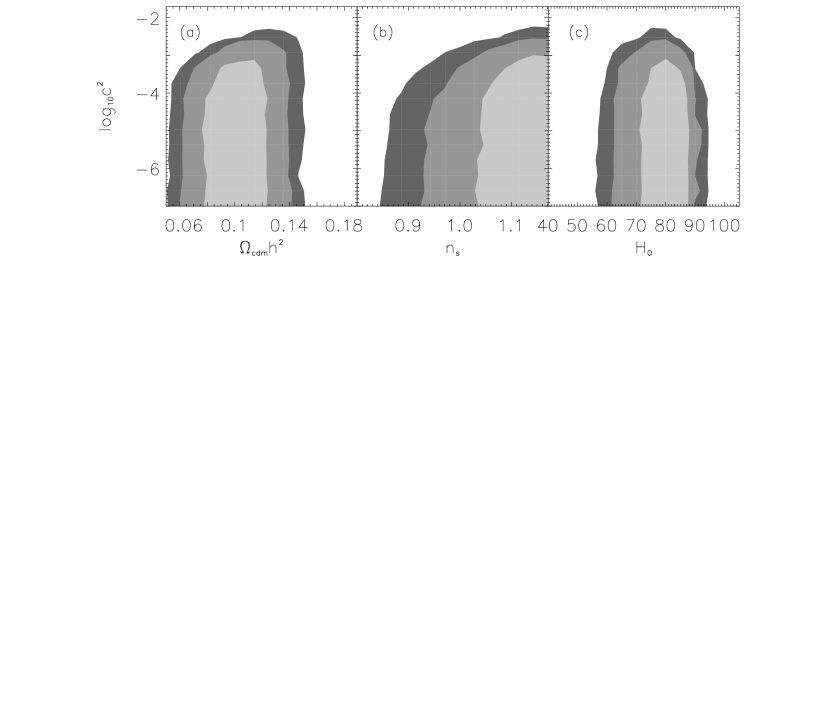
Figure 4: Marginalized likelihood function for the 2dFGRS data.

VII Discussion

Interacting quintessence models have been constructed to solve the coincidence problem. They make specific predictions that can be checked against observations of large scale structure. In this paper we have shown that the interaction induces measurable effects in the growth of the matter density perturbations and modifies the power spectrum on small scales. To summarize, if dark energy decays into dark matter the background model has less dark matter and more dark energy in the past compared to non-decaying models. Since the dark energy does not cluster on small scales it does not contribute to the growth of density perturbations. The mean free–fall time increases and perturbations grow slower than in non-interacting models. The slower growth of matter density perturbations during the radiation and matter period, results on a damping of the matter power spectrum on those scales that cross the horizon before matter-radiation equality, but it does not change the slope on large scales.

The combined effect of shifting the scale of matter radiation equality and changing the slope of matter power spectrum at small scales is a distinctive feature of interacting models where the dark energy does not cluster on small scales. Measurements of matter power spectrum could eventually reach enough statistical power to discriminate between interacting and non-interacting models. For example, the spectrum obtained from Lymann-$\alpha$ absorption lines on quasar spectra lya probe the matter power spectrum at redshifts in the interval $(2,4)$, where non-linear evolution has not yet erased the primordial information down to megaparsec scale. The use of more precise information on small and large scales, could set tighter bounds on the interaction of dark matter and dark energy.

Our previous results olivares and those presented here indicate that the IQM fits the observational data as well as non-interacting models, alleviates the coincidence problem and provides a unified picture of dark matter and dark energy. It predicts a damping on the matter power spectrum on small scales that can be used, together with the delay on the matter-radiation equality, to discriminate it from non-interacting models. The slower growth of subhorizon sized matter density perturbations within the horizon provides a clean observational test to proof or rule out a DM–DE coupling.

- (1) S. Perlmutter et al., Nature (London) 391, 51 (1998); A.G. Riess et al., Astron. J. 116, 1009 (1998); S. Perlmutter et al., Astrophys. J. 517, 565 (1999); P. de Bernardis et al., Nature (London) 404, 955 (2000); R.A. Knop et al., Astrophys. J. 598, 102 (2003); J.L. Tonry et al., Astrophys. J. 594, 1 (2003); M.V. John, Astrophys. J. 614, 1 (2004); A.G. Riess et al., Astrophys. J. 607, 665 (2004); P. Astier et al., Astron. Astrophys. 447, 31 (2006).
- (2) D.N. Spergel et al., Astrophys. J. Supl. Ser. 148, 175 (2003).
- (3) D.N. Spergel et al., astro-ph/0603449; G. Hinshaw et al., astro-ph/0603451.
- (4) M. Tegmark et al., Phys. Rev. D 69, 103501 (2004).
- (5) S. Cole et al., Monthly Not.R. Astr. Soc. 362, 505 (2005).
- (6) S. Boughn, and R. Crittenden, Nature (London) 427, 45 (2004); P. Vielva, E. Martínez González, and M. Tucci, Mon. Not. R. Astr. Soc 365, 891 (2006).
- (7) S. Carroll, in Measuring and Modelling the Universe, Carnegie Observatory, Astrophysics Series, Vol. 2, edited by W.L.Freedman (Cambridge University Press, Cambridge, 2004); T. Padmanbhan, Phys. Reports, 380, 235 (2003); V. Sahni, astro-ph/0403324; L. Perivolaropoulos, astro-ph/0601014.
- (8) S. Weinberg, Rev. Mod. Phys. 61, 1 (1988).
- (9) P.J. Steinhardt, in Critical Problems in Physics, edited by V.L. Fitch and D.R. Marlow (Princeton University Press, Princeton, NJ, 1997).
- (10) P.J.E. Peebles and B. Ratra, Rev. Mod. Phys. 75, 559 (2003).
- (11) L. P. Chimento and D. Pavón, Phys. Rev. D 73, 063511 (2006).
- (12) L. Amendola, Phys. Rev. D 62, 043511 (2000); L. Amendola and D. Tocchini-Valentini, Phys. Rev. D 64, 043509 (2001); L. Amendola and D. Tocchini-Valentini, Phys. Rev. D 66, 043528 (2002); L. Amendola, C. Quercellini, D. Tocchini-Valentini, and A. Pasqui, Astrophys. J. 583, L53(2003).
- (13) Rong-Gen Cai and Anzhong Wang, JCAP 0503(2005)002.
- (14) W. Zimdahl, D. Pavón, and L.P. Chimento, Phys. Lett. B 521, 133 (2001).
- (15) L.P. Chimento, A.S. Jakubi, D. Pavón, and W. Zimdahl, Phys. Rev. D 67, 083513 (2003).
- (16) S. del Campo, R. Herrera, and D. Pavón, Phys. Rev. D 70, 043540 (2004).
- (17) G. Farrar and P.J.E. Peebles, Astrophys. J. 604, 1 (2004).
- (18) A.W. Brookfield, C. van de Bruck, D.F. Mota, and D. Tocchini-Valentini, Phys. Rev. D 73, 083515 (2006).
- (19) G. Olivares, F. Atrio-Barandela, and D. Pavón, Phys. Rev. D 71, 063523 (2005).
- (20) M. Szydlowski, T. Stachowiak, and R. Wojtak, Phys. Rev. D 73, 063516 (2006).
- (21) L. Amendola and C. Quercellini, Phys. Rev. Lett. 92, 181102 (2004).
- (22) T. Koivisto, Phys. Rev. D 72, 043516 (2005).
- (23) C. Wetterich, Nucl. Phys. B 302, 668 (1988); Astron. Astrophys. 301, 321 (1995).
- (24) F. Piazza and S. Tsujikawa, JCAP 0407(2004)004; S. Tsujikawa and M. Sami, Phys. Lett. B 603, 113 (2004).
- (25) L. Amendola, M. Quartin, S. Tsujikawa and I. Waga, astro-ph/0605488.
- (26) See Section II in Ref.olivares .
- (27) K. Hagiwara et al., Phys. Rev. D 66, 010001 (2002).
- (28) C.P. Ma and E. Bertschinger, Astrophys. J. 455, 7 (1995).
- (29) U. Seljak and M. Zaldarriaga, Astrophys. J. 469, 437 (1996), see http://www.cmbfast.org
- (30) L. Amendola, Phys. Rev. D 69, 103524 (2004).
- (31) S. Das, P.S. Corasaniti, and J. Khoury, Phys. Rev. D 73, 083509 (2006).
- (32) T. Padmanabhan, Structure Formation in the Universe (CUP, Cambridge, 1993).
- (33) B. Ratra and P.J.E. Peebles, Phys. Rev. D 37, 3406 (1988).
- (34) L. Amendola, Phys. Rev. Lett. 93, 181102 (2004).
- (35) E.R. Harrison, Phys. Rev. D 1, 2726 (1970); Ya. B. Zeldovich, Mon. Not. R. Astr. Soc. 160, 1 (1972).
- (36) M. Davis, F.J. Summers, and D. Schlegel, Nature (London) 359, 393 (1992).
- (37) P. McDonald et al., Astrophys. J. 635, 761 (2005).