Discovery of Very High Energy $\gamma$-Ray Emission from the BL Lac Object H 2356$-$309 with the H.E.S.S. Cherenkov Telescopes

The extreme synchrotron BL Lac object H 2356$-$309, located at a redshift of $z=0.165$, was observed from June to December 2004 with a total exposure of $\approx$40 h live-time with the H.E.S.S. (High Energy Stereoscopic System) array of atmospheric-Cherenkov telescopes (ACTs). Analysis of this data set yields, for the first time, a strong excess of 453 $\gamma$-rays (10 standard deviations above background) from H 2356$-$309, corresponding to an observed integral flux above 200 GeV of I($>$200 GeV) = (4.1 $\pm$ 0.5) $\times$ 10^-12 cm^-2s^-1 (statistical error only). The differential energy spectrum of the source between 200 GeV and 1.3 TeV is well-described by a power law with a normalisation (at 1 TeV) of N₀ = ($3.00\,\pm\,0.80_{\mathrm{stat}}\,\pm\,0.31_{\mathrm{sys}}$) $\times$ 10^-13 cm^-2s^-1TeV^-1 and a photon index of $\Gamma$ = $3.09\,\pm\,0.24_{\mathrm{stat}}\,\pm\,0.10_{\mathrm{sys}}$. H 2356$-$309 is one of the most distant BL Lac objects detected at very-high-energy $\gamma$-rays so far. Results from simultaneous observations from ROTSE-III (optical), RXTE (X-rays) and NRT (radio) are also included and used together with the H.E.S.S. data to constrain a single-zone homogeneous synchrotron self-Compton (SSC) model. This model provides an adequate fit to the H.E.S.S. data when using a reasonable set of model parameters.

1 Introduction

The Spectral Energy Distribution (SED) of Active Galactic Nuclei (AGN) spans the complete electromagnetic spectrum from radio waves to very-high-energy (VHE; E $>$ 100 GeV) $\gamma$-rays. In the widely-accepted unified model of AGN (e.g. Rees, 1984; Urry & Padovani, 1995), the “central engine” of these objects consists of a super-massive black hole (up to 10⁹ M_⊙) surrounded by a thin accretion disk and a dust torus. In some radio-loud AGN, i.e. objects with a radio to B-band flux ratio F_5GHz/F_B $>$ 10, two relativistic plasma outflows (jets) presumably perpendicular to the plane of the accretion disk have been observed.

AGN are known to be VHE $\gamma$-ray emitters since the detection of Mrk 421 above 300 GeV by the Whipple group (Punch et al., 1992), who pioneered the imaging atmospheric-Cherenkov technique. At very high energies, a number of AGN ($\approx$10) were subsequently detected by different groups using a similar technique. Almost all these objects are BL Lacertae (BL Lac) objects, belonging to the class of Blazars (BL Lac objects and Flat Spectrum Radio Quasars), i.e. AGN having their jet pointing at a small angle to the line of sight. The only confirmed VHE detection of an extragalactic object not belonging to the BL Lac class is the giant radio galaxy M 87 (Aharonian et al., 2003, 2005d).

Two broad peaks are present in the observed SED of AGN. The first peak is located in the radio, optical, and X-ray bands, the second peak is found at higher energies and can extend to the VHE band. The observed broad-band emission from AGN is commonly explained by two different model types. In leptonic models, the lower-energy peak is explained by synchrotron emission of relativistic electrons and the high-energy peak is assumed to result from inverse Compton (IC) scattering of electrons off a seed-photon population, see e.g. Sikora & Madejski (2001) and references therein. In hadronic models, the emission is assumed to be produced via the interactions of relativistic protons with matter (Pohl & Schlickeiser, 2000), ambient photons (Mannheim, 1993) or magnetic fields (Aharonian, 2000), or via the interactions of relativistic protons with photons and magnetic fields (Mücke & Protheroe, 2001).

The observed $\gamma$-ray emission from BL Lac objects shows high variability ranging from short bursts of sub-hour duration to long-time activity of the order of months. Detailed studies of variability of BL Lac type objects can contribute to the understanding of their intrinsic acceleration mechanisms (e.g. Krawczynski et al., 2001; Aharonian et al., 2002). Additionally, observations of distant objects in the VHE band provide an indirect measurement of the SED of the Extragalactic Background Light (EBL), see e.g. Stecker et al. (1992); Primack et al. (1999) and references therein. Due to the absorption of VHE $\gamma$-rays via e⁺e^- pair production with the photons of the EBL, the shape of the observed VHE spectra is distorted as compared to the intrinsically emitted spectra. Using a given spectral shape of the EBL, the observed AGN spectrum can be corrected for this absorption. The resulting intrinsic (i.e., corrected) spectrum can then be compared to basic model assumptions on the spectral shape of the $\gamma$-ray emission, thereby constraining the applied shape of the EBL. In this context, it is especially important to detect AGN at higher redshifts but also to study the spectra of objects over a wide range of redshifts, in order to disentangle the effect of the EBL from the intrinsic spectral shape of the objects. To date, the redshifts of VHE emitting BL Lac objects with measured spectra range from $z=0.033$ to $z=0.129$.

The high frequency peaked BL Lac object (HBL) H 2356$-$309, identified in the optical by Schwartz et al. (1989), is hosted by an elliptical galaxy located at a redshift of $z=0.165$ (Falomo, 1991). The object was first detected in X-rays by the satellite experiment UHURU (Forman et al., 1978) and subsequently by the Large Area Sky Survey experiment onboard the HEAO-I satellite (Wood et al., 1984). The spectrum of H 2356$-$309 as observed by BeppoSAX (Costamante et al., 2001) is not compatible with a single power law model, indicating that the peak of the synchrotron emission lies within the energy range of BeppoSAX. A broken power law fit yields a synchrotron peak around 1.8 keV, with a detection of the source up to 50 keV. These observations qualified the object as an extreme synchrotron blazar.

A selection of TeV candidate BL Lac objects was proposed by Costamante & Ghisellini (2002). The objects were selected from several BL Lac samples and using information in the radio, optical and X-ray bands. VHE predictions for the selected objects were given by the authors based on a parametrisation proposed by Fossati et al. (1998), suitable for predictions of high state flux of an average source population. The authors also gave VHE flux predictions based on a simple one-zone homogeneous SSC model (Ghisellini et al., 2002), appropriate for a quiescent state of the specific VHE source candidate. H 2356$-$309 is included in this list and the predicted integral flux values above 300 GeV for H 2356$-$309 are 8.4$\times$10^-12 cm^-2s^-1 for the parametrisation and 1.9$\times$10^-12 cm^-2s^-1 for the SSC model. It should be noted that no absorption due to the EBL was taken into account in these calculations.

In this paper the discovery of VHE $\gamma$-rays from H 2356$-$309 with the H.E.S.S. Cherenkov telescopes in 2004 is reported. With a redshift of $z=0.165$, H 2356$-$309 is one of the most distant AGN detected at VHE energies so far. H 2356$-$309 was observed by H.E.S.S. from June to December 2004 (see sections 2 and 3). Simultaneous observations were carried out with RXTE (Rossi X-ray Timing Explorer) in X-rays on 11th of November 2004 (see section 4.1), with the Nançay decimetric radio telescope (NRT) between June and October 2004 (see section 4.2) and with ROTSE-III (see section 4.3) in the optical, covering the whole 2004 H.E.S.S. observation campaign.

2 H.E.S.S. Observations

The system of four H.E.S.S. ACTs, located on the Khomas Highlands in Namibia (23^∘16’18”S 16^∘30’00”E), is fully operational since December 2003. For a review see, e.g., Hinton (2004). H.E.S.S. data are taken in runs with a typical duration of 28 minutes. The data on H 2356$-$309 were taken with the telescopes pointing with an offset of 0.5^∘ relative to the object position (wobble mode, offset in either right ascension or declination). The sign of the offset is alternated for successive runs to reduce systematic effects. H 2356$-$309 was observed with the complete stereoscopic system from June to December 2004 for a total raw observation time of more than 80 hours. In order to reduce systematic effects that arise due to varying observation conditions, quality selection criteria are applied before data analysis on a run-by-run basis. The criteria are based on the mean trigger rate (corrected for zenith-angle dependency), trigger rate stability, weather conditions and hardware status. During the 2004 observations of H 2356$-$309 atmospheric conditions were not optimal (due to brushfires), resulting in a dead-time corrected high-quality data set of $\approx$40 h live-time at an average zenith angle of 20^∘.

These data are calibrated as described in Aharonian et al. (2004). Thereafter, before shower reconstruction, a standard image cleaning (Lemoine-Goumard et al., 2005) is applied to the shower images to remove night-sky background noise. Moreover, in order to avoid systematic effects from shower images truncated by the camera edge, only images having a distance between their centre of gravity and the centre of the camera of less than 2^∘ are used in the reconstruction. Furthermore, a minimum image amplitude (i.e., the sum of the intensities of all pixels being part of the image) is required for use in the analysis to assure a good quality reconstruction. Previous H.E.S.S. publications are mostly based on the standard analysis (Aharonian et al., 2005a). Here we present results from the 3D Model analysis which is presented in detail in Lemoine-Goumard et al. (2005) and was also used in Aharonian et al. (2005b). This method uses independent calibration and simulation chains and is briefly described in the following paragraphs.

2.1 H.E.S.S. 3D Model Analysis

The principle of the 3D Model reconstruction method (Lemoine-Goumard & Degrange, 2004; Lemoine-Goumard et al., 2005; Aharonian et al., 2005b) is based on a 3-dimensional (3D) shower model using the stereoscopic information from the telescopes. The shower is modelled as a 3D Gaussian photosphere with anisotropic angular distribution. For each camera pixel the expected light is calculated with a path integral along the line of sight. The observed images are then compared to the model images using a log-likelihood fit with eight parameters, described in detail in Lemoine-Goumard et al. (2005). For each detected shower at least two images are required for the reconstruction of the angle $\theta$ (the angle between the object position and the reconstructed shower direction), shower core impact position (measured as a radius with respect to the center of the telescope array), energy and the transverse standard deviation $\sigma_{T}$ of the shower. The dimensionless reduced 3D width $\omega$ (used for $\gamma$-hadron separation) is defined as $\omega=\sigma_{T}\rho/D_{S}$, with the density of air $\rho$ and the column density $D_{S}$ at shower maximum. The energy spectrum of the $\gamma$-ray excess is obtained from a comparison of the reconstructed energy distributions to the expected distributions for a given spectral shape. For the determination of the expected number, $\gamma$-ray acceptances calculated from simulations are taken into account. This forward folding method was first developed within the CAT collaboration (Piron, F., 2000). The quality of the reconstruction improves when only events with a number of triggered telescopes $N_{tel}\geq 3$ are accepted. In the analysis used in this paper, results from the 3D Model are given using this cut. A spectral analysis using an $N_{tel}\geq 2$ cut yields consistent results.

The on-source data are taken from a circular region of radius $\theta$ around the object position (on-source region). The background is estimated from 11 control regions (off-source regions) of the same size and located at the same radial distance to the camera centre as the on-source region and normalised accordingly. The significance in standard deviations above background (subsequently $\sigma$) of any excess is calculated following the likelihood method of Li & Ma (1983). All cuts applied are summarised in Table 1. Cut values were optimised using simulated $\gamma$-ray samples and independent background data samples.

Table 1: Summary of applied cuts. The cut in image amplitude is given in photoelectrons (ph.e.).

cut	value
distance	2 deg
image amplitude	$>$60 ph.e.
# of telescopes	$\geq$ 3
core impact position	$\leq$ 300 m
mean reduced scaled width	–
mean reduced scaled length	–
reduced 3D width $\omega$	$<$0.002
$\theta^{2}$	$<$0.01 deg2

3 H.E.S.S. Results

3.1 Signal

In Figure 1, the distribution of the squared angular distances $\theta^{2}$ from H 2356$-$309, reconstructed with the 3D-Model ($N_{tel}\geq 3$), is shown. In the data taken from the on-source region a clear accumulation of events is seen at low $\theta^{2}$-values, i.e. close to the position of H 2356$-$309. The off-region shows a flat distribution as expected for a pure background measurement. With a number of on-source events of ${N_{on}}$ = 1706 off-source events ${N_{off}}$ = 13784 and a normalisation factor $\alpha$=0.0909 (the ratio between the solid angles for on- and off-source measurements), the data yield an excess of ${N_{on}}$ - $\alpha$${N_{off}}$ = 453 $\gamma$-rays at a significance-level of 11.6 $\sigma$. A fit of a 2-dimensional Gaussian to an uncorrelated excess sky-map yields a point-like emission and a location (23$h$59$m$09.42$s$ $\pm$ 2.89$s$, -30^∘37’22.7” $\pm$ 34.5”) consistent with the position of H 2356$-$309 (23$h$59$m$07.8$s$, -30^∘37’38”), as obtained by Falomo (1991) using observations in the optical and near-infrared.

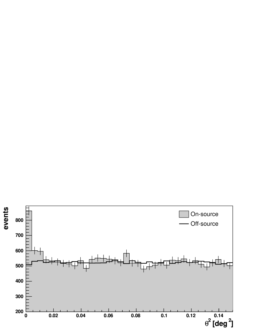
Figure 1: Distribution of squared angular distances $\theta^{2}$ for H 2356$-$309, using the 3D-Model reconstruction and $N_{tel}\geq 3$.

These results are summarised in Table 2. Additionally, the results from the standard analysis are given. The results for the 3D Model analysis used in this paper are also given using $N_{tel}\geq 2$ for easier comparison with the standard analysis.

Table 2: Summary of analysis results from the 3D Model analysis (using two different cuts in telescope multiplicity). For comparison, the standard analysis results are also given.

	3D Model		standard analysis
	$N_{tel}\geq 3$	$N_{tel}\geq 2$	$N_{tel}\geq 2$
${N_{on}}$ (events)	1706	4389	3776
${N_{off}}$ (events)	13784	40420	35280
normalisation $\alpha$	0.0909	0.0909	0.0903
Excess (events)	453	715	591
Significance	11.6 $\sigma$	10.9 $\sigma$	9.7 $\sigma$

3.2 Energy Spectrum and Variability

The differential energy spectrum obtained from the 3D-Model analysis ($N_{tel}\geq 3$) is shown in Figure 2. The spectral parameters were obtained from a maximum likelihood fit of a power law hypothesis $dN/dE=N_{0}(E/\mathrm{TeV})^{-\Gamma}$ to the data, resulting in a flux-normalisation of N₀ = ($3.00\,\pm\,0.80_{\mathrm{stat}}\,\pm\,0.31_{\mathrm{sys}}$) $\times$ 10^-13 cm^-2s^-1TeV^-1, and a spectral index of $\Gamma$ = $3.09\,\pm\,0.24_{\mathrm{stat}}\,\pm\,0.10_{\mathrm{sys}}$. The $\chi^{2}$ value of the spectral fit is 6.6 for 7 degrees of freedom, corresponding to a $\chi^{2}$-probability of $P(\,\chi^{2})$ = 0.47. In order to eliminate any systematic effects that might arise from poor energy estimation at lower energies (due to an over-estimation, on average, of low energies), the beginning of the fit range is set to the value of the post-cuts spectral energy threshold, i.e. 200 GeV for the 3D Model analysis of this data set. Systematic errors (0.1 for the index and 20 % for the flux) are dominated by atmospheric effects, i.e. a limited knowledge of the atmospheric profile needed as input for the simulations. A detailed description of systematic errors can be found in e.g., Aharonian et al. (2006). The parameters of the spectral fit are summarised in Table 3. Additionally, the results from the standard analysis are given for comparison. The data-points used in Figure 2 are listed in Table 4.

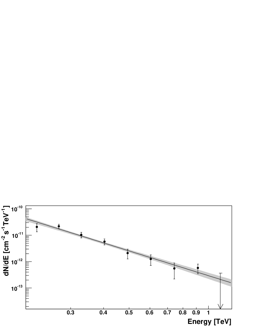
Figure 2: Differential energy spectrum of H 2356$-$309, as obtained from the 3D Model analysis. The shaded area gives the confidence region (1 standard deviation) for the spectral shape under the assumption of a power law. The upper limit (arrow) is given with a 99 % confidence level.

Table 3: Summary of the parameters of power law fits ($dN/dE=N_{0}(E/\mathrm{TeV})^{-\Gamma}$). For comparison with the 3D Model analysis (1) used here, the results from the standard analysis (2) are also given. Both analyses yield consistent results. In addition to the parameter values, the $\chi^{2}$ probabilities of the fits are given.

	$\Gamma$	${N_{0}}$	${P(\,\chi^{2})}$
		$[$10-13 cm-2s-1TeV-1$]$
(1)	$3.09\,\pm\,0.24_{\mathrm{stat}}\,\pm\,0.10_{\mathrm{sys}}$	$3.00\,\pm\,0.80_{\mathrm{stat}}\,\pm\,0.31_{\mathrm{sys}}$	0.47
(2)	$3.06\,\pm\,0.21_{\mathrm{stat}}\,\pm\,0.10_{\mathrm{sys}}$	$3.07\,\pm\,0.75_{\mathrm{stat}}\,\pm\,0.31_{\mathrm{sys}}$	0.60

Table 4: Differential flux for different energy bins. The upper limit is given for a confidence level of 99 %.

E	$\Phi$	$\Delta\Phi$
$[$TeV$]$	$[$cm-2s-1TeV-1$]$
0.223	2.06$\,\times\,10^{-11}$	7.13$\,\times\,10^{-12}$
0.270	2.18$\,\times\,10^{-11}$	4.36$\,\times\,10^{-12}$
0.329	1.04$\,\times\,10^{-11}$	2.46$\,\times\,10^{-12}$
0.403	5.77$\,\times\,10^{-12}$	1.48$\,\times\,10^{-12}$
0.494	2.12$\,\times\,10^{-12}$	8.51$\,\times\,10^{-13}$
0.604	1.26$\,\times\,10^{-12}$	5.45$\,\times\,10^{-13}$
0.742	5.50$\,\times\,10^{-13}$	3.29$\,\times\,10^{-13}$
0.912	5.77$\,\times\,10^{-13}$	2.31$\,\times\,10^{-13}$
1.113	$<$4.06$\,\times\,10^{-13}$	–

The average integral flux above 200 GeV in the year 2004 (fitting with a fixed spectral index of 3.09) is $\overline{I(>200\,\mathrm{GeV})}$ = (4.1 $\pm$ 0.5) $\times$ 10^-12 cm^-2s^-1 (statistical error only). Light-curves of I($>$200 GeV) versus the modified Julian date (MJD) of the observation are shown in Figure 3 for two different time-scales. The monthly flux variation is shown in the upper panel and the average monthly flux from June to December of 2004 is shown in the lower panel. A fit of a constant yields no evidence for nightly variability (P( $\chi^{2}$)=0.18).

The ASM (All Sky Monitor) shows no significant X-ray excess nor variability in the same monthly intervals.

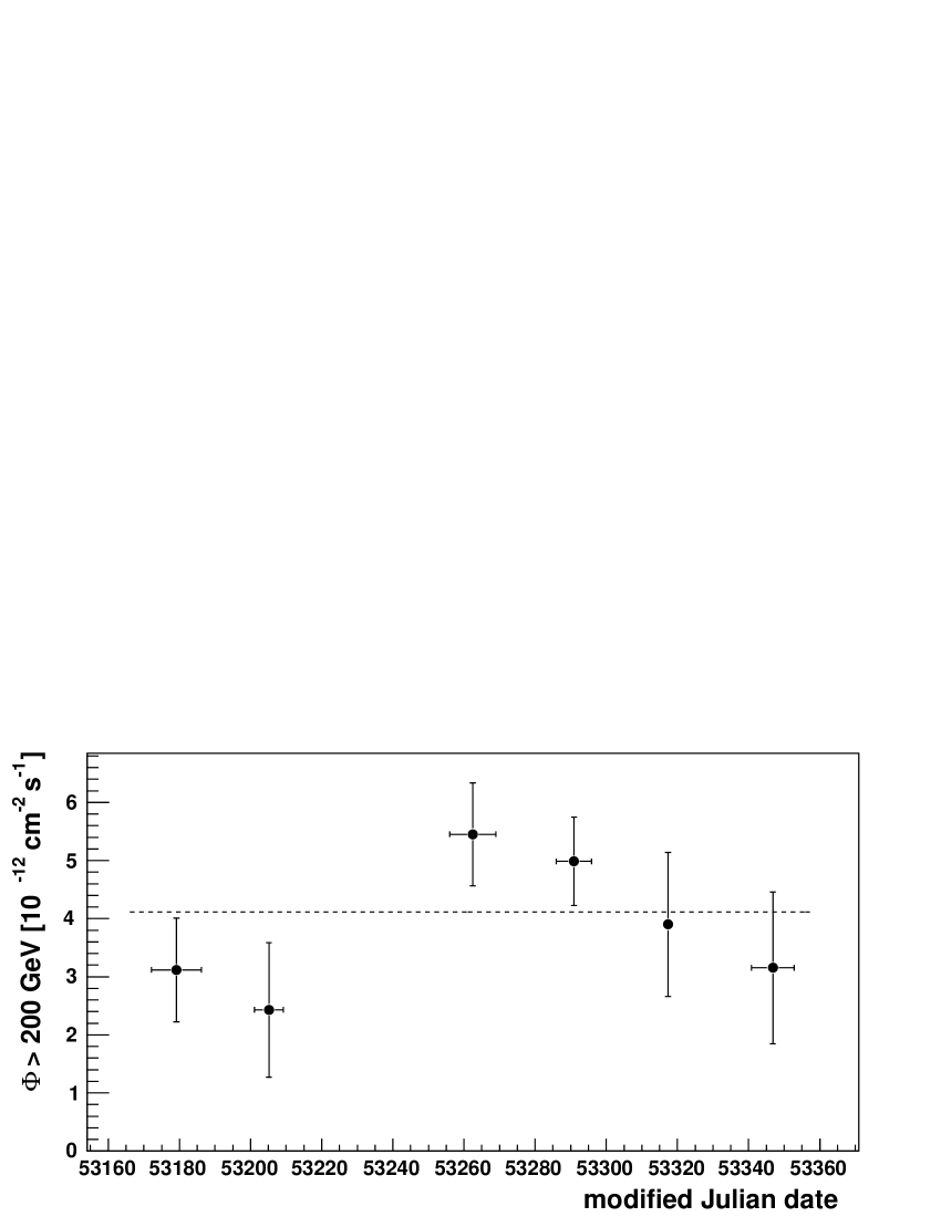
Figure 3: Flux above 200 GeV from H 2356$-$309 as measured by H.E.S.S. (3D Model Analysis) in 2004. Upper panel: each point corresponds to the flux measurement in one night. Lower panel: averaged flux in six different time windows (June to December 2004). Both light-curves are consistent with a constant emission over time. The RXTE observations (see Section 4.1) were carried out on MJD 53320. During that night, no H.E.S.S. observations could take place due to poor weather conditions.

4 Multi-Wavelength Analysis and Results

4.1 RXTE analysis

The RXTE/PCA (Jahoda & PCA Team, 1996) observed H 2356$-$309 twice for a total of 5.4 ks on 11 November 2004 after a Target of opportunity was triggered on this target. Due to poor weather conditions, H.E.S.S.-observations were not possible on the night of November 11, or on the 2 prior nights. However, the RXTE observations can be considered simultaneous to the H.E.S.S. observation campaign of November. The STANDARD2 data were extracted using the ftools in the HEASOFT 6.0 analysis software package provided by NASA/GSFC and filtered using the RXTE Guest Observer Facility recommended criteria. Only the signals from the top layer (X1L and X1R) are used from the PCA. The average spectrum shown in the SED (Figure 4) is derived by using PCU0, PCU2 and PCU3 data. The faint-background model is used and only the 3–20 PHA channel range is kept in XSPEC v. 11.3.2, or approximately 2–$10\,\rm keV$. The column density is fixed to the Galactic value of $N_{\rm H}=1.33\times 10^{20}\,\rm cm^{-2}$ obtained from the PIMMS nH program and is used in an absorbed power law fit. This yields an X-ray photon index $\Gamma_{X}=2.43\pm 0.11$ and a flux of $9.7^{+0.3}_{-1.3}\times 10^{-12}\,\rm erg\,cm^{-2}\,s^{-1}$ in the 2–$10\,\rm keV$ band. The $\chi^{2}$ of the fit is 11 for 14 degrees of freedom, or a $\chi^{2}$ probability $P(\,\chi^{2})=0.68$. This flux level is approximately a factor of 3 lower than what was reported from BeppoSAX observations by Costamante et al. (2001) and with a softer photon index than what was observed above 2 keV.

4.2 NRT analysis

The Nançay radio-telescope is a single-dish antenna with a collecting area of $200\times 34.56$ m² equivalent to that of a $94\,{\rm m}$-diameter parabolic dish (van Driel et al., 1996). The half-power beam width at $11\,\rm cm$ is $1.9\,{\rm arcmin}$ (EW) $\times 11.5\,{\rm arcmin}$ (NS) (at zero declination), and the system temperature is about $45\,\rm K$ in both horizontal and vertical polarisations. The point source efficiency is $0.8\,{\rm K}\,{\rm Jy}^{-1}$, and the chosen filter bandwidth was 12.5 MHz for each polarisation, split into two sub-bands of 6.25 MHz each. Data were processed using the Nançay local software NAPS and SIR.

A monitoring program with this telescope on extragalactic sources visible by both the NRT and H.E.S.S. is in place since 2001. For the campaign described here it consisted of a measurement at $11\,\rm cm$ every two or three days. Between 4 and 14 individual 1-minute drift scans were performed for each observation, and the flux calibration was done using a calibrated noise diode emission for each drift scan. The average flux for the measurements carried out between 11 June and 10 October 2004 was $40\pm 8\,\rm mJy$. This observed flux is most likely dominated by emission produced in jet regions further out from the core and thus represents an upper limit of any emission model for the total SED.

4.3 ROTSE-III Analysis

The ROTSE-III (Robotic Optical Transient Search Experiment) array is a world-wide network of four 0.45 m robotic, automated telescopes built for fast ($\approx$ 6 s) response to GRB triggers from satellites such as HETE-2 (High Energy Transient Explorer 2) and Swift. The ROTSE-III telescopes have a wide ($1.85^{\circ}\times 1.85^{\circ}$) field of view imaged onto a Marconi 2048 $\times$ 2048 pixel back-illuminated thinned CCD and are operated without filters. The ROTSE-III systems are described in detail in Akerlof et al. (2003). The ROTSE-IIIc telescope, located at the H.E.S.S. site, has been used to perform an automated monitoring programme of blazars, including H 2356$-$309. Data is analysed as described in Aharonian et al. (2005c) and references therein. During the observation periods covered by H.E.S.S. the apparent R-band magnitude m(R) from H 2356$-$309 as measured by ROTSE-III has its maximum at m(R) = 16.1 and its minimum at m(R) = 16.9. The host galaxy has been resolved in the optical (Falomo, 1991; Scarpa et al., 2000) and near-infrared (Cheung et al., 2003). These observations show that H 2356$-$309 is a normal elliptical galaxy with an effective radius of about 1.8 arcsec in the R band. The contribution of the galaxy to the observed ROTSE-III flux is estimated to be m(R) = 17 using a standard de Vaucouleurs radial profile.

5 Discussion

In Figure 4, a broad-band SED obtained from archival data, and simultaneous optical (ROTSE-III) and X-ray (RXTE) data together with the H.E.S.S. results presented in this paper is shown. Additionally, the result of a simple leptonic model is given as a solid line. The simplest leptonic scenario is a one-zone homogeneous, time independent, synchrotron self-Compton (SSC) model as initially proposed by Jones et al. (1974) for compact non-thermal extragalactic sources.

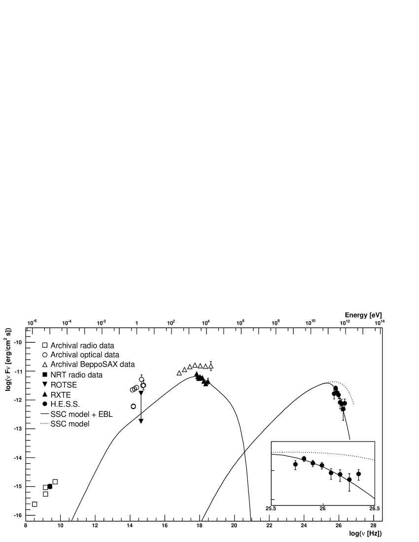
Figure 4: Spectral energy distribution of H 2356$-$309. Above 200 GeV, the results obtained in this paper are used. Data from NRT, ROTSE-III and RXTE are simultaneous to the H.E.S.S. observations and shown as filled symbols. All other data are archival and shown as open symbols. The ROTSE-III flux is given after galaxy subtraction. Radio emission arises from regions further out in the jet. A single-zone homogeneous SSC model described in the text is shown as a solid line. The dashed line shows the SSC model without absorption. The inlaid box shows a zoom in the VHE regime.

Here, we adopt a description with a spherical emitting region of radius $R$ and homogeneous magnetic field $B$, propagating with Doppler factor $\delta$ with respect to the observer. The high energy electron distribution is described by a broken power law between Lorentz factors $\gamma_{\rm min}$ and $\gamma_{\rm max}$, with a break at $\gamma_{\rm b}$ and a normalisation $K$ (Katarzyński et al., 2001). This SSC scenario is used, taking into account absorption by the EBL, to reproduce the simultaneous data of H 2356$-$309. The density of the EBL is not well known in the $\mu$m wavelength regime. Given the high redshift of H 2356$-$309 ($z=0.165$) and a comparatively hard VHE spectrum, important constraints on the EBL density can be derived from the H.E.S.S. data. This question is addressed in detail in Aharonian et al. (2005e) where constraints on the density of the EBL are derived from H.E.S.S. observations of 1ES 1101$-$232 and H 2356$-$309. Here, we use the P0.45 parametrisation from this paper which is very close to the lower limit from galaxy counts.

As shown in Figure 4, using a model with a reasonable set of parameters provides a satisfactory fit to the simultaneous x-ray and VHE data. The emitting region is characterised by $\delta=18$, $B=0.16$ G and $R=3.4\,\times\,10^{15}$ cm. The electron power-law distribution is described by $K=1.2\,\times\,10^{4}$ cm^-3, $\gamma_{\rm min}=10^{3}$, $\gamma_{\rm max}=3\,\times\,10^{6}$. The Lorentz factor at break energy $\gamma_{\rm b}$ is located at $\gamma_{\rm b}=2.5\,\times\,10^{5}$ to place the peak emission in between optical and X-rays while providing a good fit to the H.E.S.S. data. We take the canonical index $\alpha_{1}$=2 for the low-energy end and found $\alpha_{2}$=4.0 for the high-energy end so as to fit the observed X-ray power law spectrum. Lowering $\gamma_{\rm min}$ extends the fit to lower frequencies and enhances IC emission in the MeV-GeV domain. Synchrotron self-absorption cuts off emission below IR frequencies when using low values of $\gamma_{\rm min}$. Radio emission arises from regions further out in the jet. Similar to the case of PKS 2155-304 (Aharonian et al., 2005c) we cannot exclude a possible contribution of such an extended region to the optical flux measured by ROTSE-III. This may soften some of the above-mentioned constraints.

Although our VHE observations provide strong constraints on the physical parameters of single-zone SSC models, there is still some freedom of choice for the parameters that could be constrained further by a better understanding of the origin of the optical emission, a better spectral coverage in the X-ray and sub-TeV region and the observation of possible variability..

6 Conclusions

The high frequency peaked BL Lac object H 2356$-$309, located at a redshift of $z=0.165$, was discovered in the VHE regime by the H.E.S.S. Cherenkov telescopes. Two different reconstruction and analysis methods were applied to the data both yielding consistent results. No strong evidence for variability in the VHE band is found within the H.E.S.S. observations. The same holds true in the X-ray band, where the object does not show any strong flux variability, neither in the ASM nor in the pointed observations. Additionally, the RXTE flux, observed simultaneously to the H.E.S.S. observations, is lower than the previously-measured BeppoSAX flux. This might indicate that our observations took place during a relatively low state of emission.

For the first time, an SED comprising simultaneous radio, optical, X-ray and VHE measurements was made. A simple one-zone SSC model, taking into account absorption by the EBL (Aharonian et al., 2005e), provides a satisfactory description of these data.

Given the high redshift of the object, the observed H.E.S.S. spectrum provides strong constraints on the density of the EBL (Aharonian et al., 2005e). Future observations of H 2356$-$309 with H.E.S.S. will improve the accuracy of the spectral measurement and might also allow an extension of the observed spectrum to higher energies. This will provide further constraints on the absorption of $\gamma$-rays by the EBL.