Arcfinder: An algorithm for the automatic detection of gravitational arcs

We present an efficient algorithm designed for and capable of detecting elongated, thin features such as lines and curves in astronomical images, and its application to the automatic detection of gravitational arcs. The algorithm is sufficiently robust to detect such features even if their surface brightness is near the pixel noise in the image, yet the amount of spurious detections is low. The algorithm subdivides the image into a grid of overlapping cells which are iteratively shifted towards a local centre of brightness in their immediate neighbourhood. It then computes the ellipticity for each cell, and combines cells with correlated ellipticities into objects. These are combined to graphs in a next step, which are then further processed to determine properties of the detected objects. We demonstrate the operation and the efficiency of the algorithm applying it to HST images of galaxy clusters known to contain gravitational arcs. The algorithm completes the analysis of an image with $3000\times 3000$ pixels in about 4 seconds on an ordinary desktop PC. We discuss further applications, the method’s remaining problems and possible approaches to their solution.

1 Introduction

Gravitational arcs are an important diagnostic for the innermost mass distribution in galaxy clusters, and thus they are an important indirect diagnostic for a variety of questions in cosmology and structure formation. So far, they have been detected almost exclusively by visual inspection of cluster images, although algorithms for their automated search have recently been proposed (Lenzen et al. 2004; Horesh et al. 2005; Alard 2006).

There are several good reasons to search for ways to detect arcs in an automated fashion. First, the unambiguous definition of arc samples calls for an objective and reliable way to detect arcs and quantify their properties. Second, wide-field surveys such as the Canada-France-Hawaii Legacy Survey combine huge data fields with sufficient depth to reach below the detection limit for arcs with their typically low surface brightness. For arc statistics and its potential importance for cosmological studies or investigations of cluster dynamics, objectively searching for arcs in these wide-field images promises an important step forward. However, scanning wide-field data by eye covering hundreds of square degrees for arcs with their typical widths of $\lesssim 1^{\prime\prime}$ and lengths of $\lesssim 10^{\prime\prime}$ appears as a hopeless endeavour.

Automated arc searches can be conducted where clusters have previously been identified, e.g. through their optical appearance or X-ray emission, but they can and should profitably be extended to blind searches on large areas. Obviously, such goals can only be pursued if an algorithm for automated arc detection is available.

The surface brightness of gravitational arcs is typically close to the background, which may vary across the image. This is one reason why we propose a new algorithm here rather than using one of those that were described and implemented earlier. For instance, the anisotropic diffusion underlying the algorithm by Lenzen et al. bears the risk of creating elongated features from the noise which may then be hard to distinguish from real arcs. Moreover, we aim at an algorithm which is simple, thus presumably robust, and fast enough to be applied to large data fields. This rules out better studied techniques for the detection of line-like features in images, such as the Hough transform. Finally, the algorithm must be capable of distinguishing artifacts such as diffraction spikes or parts thereof from arcs. As we shall show below, the algorithm proposed here does indeed satisfy these criteria.

2 Approach

We begin the description of our algorithm by summarising what it is supposed to achieve. Next, we shall explain the numerical methods used and the reasons for employing them.

2.1 General description

We want the algorithm to identify features in astronomical images with the following properties:

1. having a higher mean pixel intensity than the surrounding background, including faint features with a mean pixel intensity well within the domain of the pixel noise where segmentation by an intensity threshold is impractical;

2. being much longer than wide, more precisely being elongated in the sense that it is possible at each point within a feature to find a local direction along which the feature’s intensity changes much less than perpendicular to it;

3. being extended in the sense that the feature’s local curvature, i.e. its change of orientation per unit length along its principal direction, is small.

According to this definition, a ring with a circumference of 100 units (e.g. pixels) and a width of 5 units should be detected as one feature, the equally narrow sides of an equilateral triangle of comparable size should be detected as three features because of the high curvature at its vertices, and an approximately circular object with a length-to-width ratio near unity should not be detected at all.

Figure 1: Small section of an HST/WFPC2 observation of Abell 2390 showing three arcs. Considerable substructure is visible in the straight arc on the left side.

Bearing strong gravitational lensing in mind, such features may be considerably substructured, which argues for choosing a detection scale limiting the size of detections to features exceeding a certain length, while structures on smaller scales should be ignored. Another reason for limiting the detection scale from below is the contamination of images with numerous elongated features generated by noise which are typically only a few pixels long.

A straightforward approach to remove small-scale structures is to initially convolve the image with a sufficiently large, isotropic kernel function, and to apply all further computations to the convolved image. However, while the convolution enhances the signal-to-noise ratio per pixel, it tends to blur and remove faint and thin features, besides being computationally expensive. It is interesting to note, and easy to see in a Fourier representation, that in an image convolved with a Gaussian kernel, fluctuations of decreasing size become increasingly unlikely.

We thus follow a different approach. We first directly compute the particular image property we are interested in as local average within areas corresponding to the detection scale. This avoids the blurring effect of an initial Gaussian convolution, but retains its positive aspects, in particular the suppression of substructures and the enhancement of the signal-to-noise ratio. It also significantly decreases the execution time because averages are only calculated for a limited set of pixels instead of all image pixels, assuming slow variations of the image property spatially close to the pixels in the set. Since they are interdependent, both the particular image property chosen for the algorithm and the selection of the set of pixels will be detailed later.

Since different local image properties, for example the smoothed intensity or its gradient, will typically vary on different scales, a smooth spatial variation on a single scale cannot generally be assumed for all local image properties one may be interested in. For example, while the intensity gradient will turn by $180^{\circ}$ when the position is shifted by a few pixels to opposite sides of a local intensity maximum, the smoothed intensity will hardly be affected by the same spatial shift. The specific characteristics chosen for detecting features must thus be taken into account in the original selection of the pixel set.

In the following, pixels combined in a set, together with their respective neighbourhoods used to compute local averages of certain image properties, are called cells. The cells’ centre coordinates vary and initialise the pixel set prior to each step of the algorithm. Even when averaged within a single cell, local image properties turn out to be insufficient for identifying faint features in presence of noise. Thus, analogous to lines of magnetic flux visible in the pattern of iron filings sprinkled on a slab of glass, the similarity of properties among groups of cells in the presence of a feature is used as the main criterion in our algorithm.

2.2 Ellipticities and cell transport

The average local pixel intensity of a feature can vary along its length, with the only limitation that it must exceed the brightness of the background. Thus, it is clearly not a good image property to use, even if most of the background could be ignored after a preselection of possible features above a minimal brightness threshold. Besides, this is problematic in itself because valid features may be fainter than typical variations in the image background.

However, since the local curvature in the direction of a valid feature is small by definition, and a flat background has no preferential orientation, directions in the local brightness pattern are a sound criterion for a detection based on local correlations between image pixels. Since the brightness gradient points into opposite directions on opposite sides of the feature, spatially averaging over it will eliminate the signatures of faint features. Using either the gradient or the structure tensor, which is the Cartesian product of the gradient with itself, is thus a problematic detection method for thin features and reasonably large scale sizes.

Instead, one can compute the direction from the ellipticity given by the second brightness moments. Let $I(\@vec{x})$ be the intensity at the position $\@vec{x}=(x_{1},x_{2})$ and $q$ an appropriately chosen weight function. Then, the weighted centre-of-brightness in an area $A$ is

$$\bar{\@vec{x}}=\frac{\int_{A}\@vec{x}q(I(\@vec{x}))\,\mathrm{d}^{2}x}{\int_{A}q(I(\@vec{x}))\,\mathrm{d}^{2}x}\;.$$ (1)

For example, $q(I(\@vec{x}))=I(\@vec{x})$ will return the unweighted centre-of-light. The tensor of second brightness moments has the components

$$Q_{ij}=\frac{\int_{A}(x_{i}-\bar{x}_{i})(x_{j}-\bar{x}_{j})q(I(\@vec{x}))\,\mathrm{d}^{2}x}{\int_{A}q(I(\@vec{x}))\,\mathrm{d}^{2}x}$$ (2)

with $i,j\in\{1,2\}$. The complex ellipticity is

$$\chi=\frac{Q_{11}-Q_{22}+2\mathrm{i}Q_{12}}{Q_{11}+Q_{22}}\;.$$ (3)

If $I(\@vec{x})$ has elliptical isophotes in $A$ with an axis ratio of $r\leq 1$, then $\chi=(1-r^{2})/(1+r^{2})\,\exp(2\mathrm{i}\vartheta)$, where $\vartheta$ is the orientation of the major axis of the elliptical isophotes relative to the $x_{1}$ axis. $\chi$ is invariant under rotations of $\pi$, as it should be because they leave ellipses unchanged.

A vector $\@vec{e}$ pointing into the direction of the major axis can be obtained by bisecting the phase angle of $\chi$ (see Appendix A),

$$\@vec{d}=\begin{cases}(\chi_{1}+|\chi|,\chi_{2})&\mbox{for}\quad\chi_{1}\geq 0\\ (\chi_{2},|\chi|-\chi_{1})&\mbox{for}\quad\chi_{1}<0\\ \end{cases}\quad\mbox{and}\quad\@vec{e}=\frac{\@vec{d}}{|\@vec{d}|}\;.$$ (4)

The orientation obtained in this way is more stable against changes in the scale size than gradient-based methods and has a higher signal-to-noise ratio because the second brightness moments are typically computed near a feature’s centre-of-brightness.

For recognising multiple features in an astronomical image without a priori information on their positions, it is obviously necessary to process the entire image initially. Our algorithm starts with cells evenly distributed and convering the image completely. Higher sensitivity can be achieved if neighbouring cells overlap, but a large overlap should be avoided to reduce the number of necessary operations on the image.

The first step in measuring the ellipticity is finding the centre of brightness as in Eq. (1). For a feature at or near the edge of a cell, the centre cannot be accurately determined in a single computation of $\bar{\@vec{x}}$. For example, when applied once to a smoothed vertical line with a Gaussian brightness profile on an already estimated background $I_{0}$,

$$I(\@vec{x})=I(x_{1})=I_{0}+\mathrm{e}^{-x_{1}^{2}/2\sigma^{2}}\;,$$ (5)

with a weight function $q(I)=I-I_{0}$ and an area $A$ extending from $0$ to $4\sigma$ in the $x_{1}$ direction, Eq. 1 yields

$$\bar{x}_{1} = \left(\int_{0}^{4\sigma}x_{1}\mathrm{e}^{-x_{1}^{2}/2\sigma^{2}}\mathrm{d}x_{1}\right)\left(\int_{0}^{4\sigma}\mathrm{e}^{-x_{1}^{2}/2\sigma^{2}}\mathrm{d}x_{1}\right)^{-1}$$ (6)

$$= -\left(\left.\sigma^{2}\mathrm{e}^{-x_{1}^{2}/2\sigma^{2}}\right|_{0}^{4\sigma}\right)\left(\left.\sigma\sqrt{\frac{\pi}{2}}\mathrm{erf}(\frac{x_{1}}{\sigma\sqrt{2}})\right|_{0}^{4\sigma}\right)^{-1}\approx 0.798\sigma\;.$$

The result improves if $\bar{\@vec{x}}$ is computed several times, each time shifting the cell’s centre to the position $\bar{\@vec{x}}$ found in the last iteration. In our example, this yields approximate centre positions $\bar{x}_{1,0}=2\sigma$, $\bar{x}_{1,1}\approx 0.798\sigma$, $\bar{x}_{1,2}\approx 0.210\sigma$, $\bar{x}_{1,3}\approx 0.048\sigma$, $\bar{x}_{1,4}\approx 0.011\sigma$ and $\bar{x}_{1,5}\approx 0.002\sigma$ after five iterations, where the second subscript denotes the iteration number.

Figure 2: Another section from the HST/WFPC2 image used for Figure 1, now centred on the optical emission of Abell 2390, showing cell paths leading to the closest local centres of brightness. The faint diagonal line crossing the image from the bottom left to the top right is a diffraction spike from a nearby foreground star.

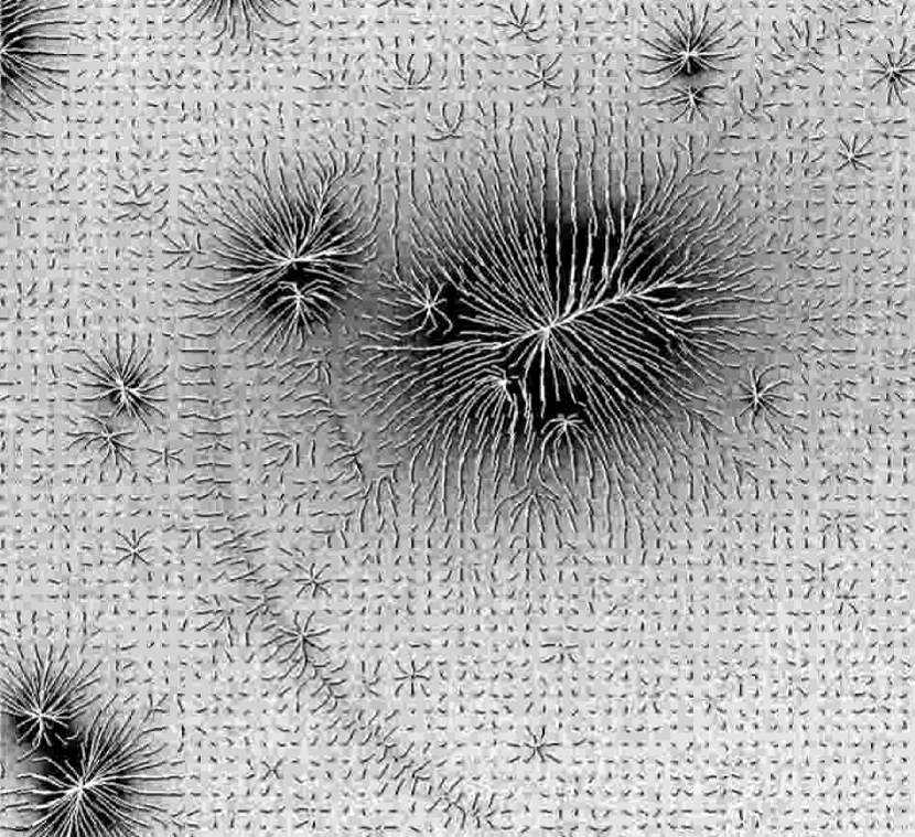
In order to allow meaningful later correlation measurements between cells, shifting initially neighbouring cells to exactly the same final position must be avoided, since there the ellipticities would then necessarily be equal regardless of a feature’s real properties. Ideally, the cells should instead be distributed equally along the feature’s main axis at the end of their iterative motion. More precisely, they should end up on or near the feature’s ridge line, i.e. the line parallel to its local directions along the brightness maxima measured perpendicular to these directions.

Carrying out too many iteration steps may create paths converging on local maxima due to substructures in the feature, while too few may leave $\bar{\@vec{x}}$ far from the ridge line. In the worst case, this may result in an orientation $\@vec{e}$ perpendicular to the feature for cells in areas characterised by a positive second derivative in the intensity profile perpendicular to the ridge line such as “valleys” between neighbouring maxima. This is because the orientation $\@vec{e}$ tends to be perpendicular to the direction of maximum intensity curvature (the secondary brightness moments $Q_{ij}$ vanish for an intensity linearly dependend on both coordinates). In the case of a Gaussian intensity profile, the effect would be visible if cells ended up more than one $\sigma$ away from the ridge line. Thus, some compromise has to be achieved. Typically, about three to four iterations have the desired effect.

It is important to note that this method is invariant under a linear scaling of the relevant weighted intensities. In the current implementation of the algorithm, $q(I)=\mathrm{max}(I-\bar{I},0)$ is used for the determination of the centre-of-brightness, where $\bar{I}$ is the mean intensity in $A$, leaving the method also invariant under a constant offset to $I$ and, more importantly, leading to a reasonably fast convergence towards the ridge line.

2.3 Correlation of neighbouring cells

Once the cells have been shifted to their new centre positions $\@vec{x}$, normalised directional vectors $\@vec{e}$ can be readily calculated using Eqs. (2) through (4), where the weight function $q(I)=I-\bar{I}$ is used for determining the second brightness moments $Q_{ij}$. Cells not initially near a feature and on a mostly flat background move randomly by short distances due to the noise, and their orientations will also be random, while cells originally located near a feature will arrive at different positions along its ridge, with very similar local orientations.

Figure 3: Cell orientations are displayed in the same area shown in Figure 2. Bold white lines mark orientations with $c^{i}\geq c_{\mathrm{th}}$.

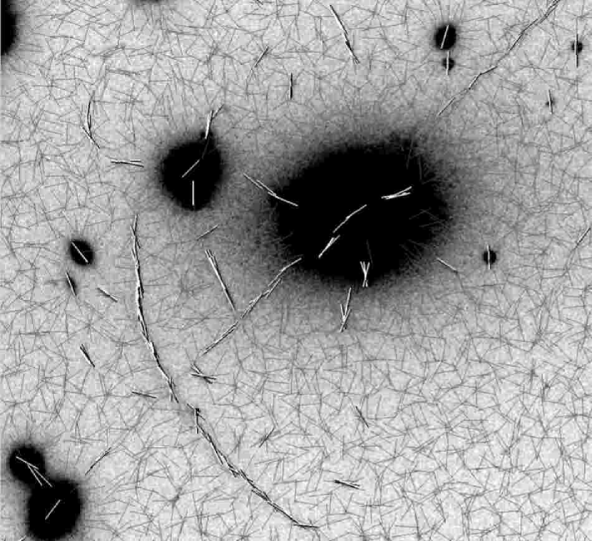
In the following, superscripts will enumerate the cells. In one dimension, the cells’ relative spatial ordering is obviously preserved: if $x^{i}_{0}<x^{j}_{0}$, then $x^{i}_{n}\leq x^{j}_{n}$ after any number $n$ of iterations of the centre computation. This is not generally true in two or more dimensions, but the number of exceptions remains negligible for small $n$. Therefore, the set $\mathcal{N}$ of neighbouring cells of a cell at the end of its path is assumed to be the same as at the beginning of its path.

Both spatial and directional information should now be used to determine whether a cell is likely to be part of a valid feature or not. To this end, we study the correlation of a cell $i$ with its neighbours $j\in\mathcal{N}$.

The similarity of orientations between cells can be expressed by

$$c_{d}^{ij}=|\@vec{e^{i}}\cdot\@vec{e}^{j}|\;.$$ (7)

The relative coordinates of the cell $j$ in an orthonormal coordinate frame centred on cell $i$ with its $x_{1}$ axis parallel to $\@vec{e}^{i}$ are

$$\@vec{\Delta}^{\prime}=\@vec{x}^{j}-\@vec{x}^{i}\quad\mbox{and}\quad\@vec{\Delta}=\left(\begin{array}[]{rcr}\Delta_{1}^{\prime}e_{1}^{i}&+&\Delta_{2}^{\prime}e_{2}^{i}\\ -\Delta_{1}^{\prime}e_{2}^{i}&+&\Delta_{2}^{\prime}e_{1}^{i}\\ \end{array}\right)\;.$$ (8)

The coordinate $\Delta_{2}$ measures the distance cell $j$ from a possible feature through the centre of cell $i$ pointing towards $\@vec{e}^{i}$. For convenience, we introduce a measure in the range $[0,1]$,

$$c_{x}^{ij}=\begin{cases}1-\frac{|\Delta_{2}|}{d_{1}}&\mbox{for}\quad|\Delta_{2}|<d_{1}\\ 0&\mbox{else}\\ \end{cases}\;,$$ (9)

where $d_{1}$ is the initial distance between neighbouring cells.

Using only the orientation and distance correlations $c^{ij}_{d}$ and $c^{ij}_{x}$, it is already possible to estimate the correlation $c^{ij}=c_{d}^{ij}c_{x}^{ij}$ between the cells $i$ and $j$ reasonably well. Including the entire neighbourhood, this becomes

$$c^{i}=\frac{1}{|\mathcal{N}|}\,\sum_{j\in\mathcal{N}}c^{ij}\;,$$ (10)

where $|\mathcal{N}|$ denotes the number of cells in the neighbourhood $\mathcal{N}$.

To reduce the effect of possible errors due to the assumption of an identical initial and final neighbourhood, and to lower the weight of closely neighbouring cells, $\mathcal{N}$ can be extended and another factor $c^{ij}_{\Delta}$ depending only on $|\Delta|$ can be introduced which is small for $|\Delta|=0$, tends to zero for $|\Delta|\gg d_{1}$, and has a maximum in $(0,d_{1}]$. For a sufficiently large initial $\mathcal{N}$, the modified correlation measure

$$c_{\Delta}^{i}=\frac{\sum_{j\in\mathcal{N}}c_{\Delta}^{ij}c^{ij}}{\sum_{j\in\mathcal{N}}c_{\Delta}^{ij}}$$ (11)

becomes independent of the initial neighbourhood and allows suppressing the contribution to the correlation of cells very close to cell $i$. Since it slightly increases the execution time, introduces an additional degree of freedom and leaves the suitable form for $c^{ij}_{\Delta}$ to be determined, this distance weighting was ignored here.

Values $c^{i}$ are computed from (10) for each cell, restricting the neighbourhood to the eight surrounding cells. Cells with $c^{i}<c_{\mathrm{th}}$ are excluded from the further processing. For many applications, a reasonable value for the threshold is $c_{\mathrm{th}}=0.5$. In a next step, those cells above the threshold which are likely part of a feature are grouped into objects, using a very similar method as described above.

2.4 Object generation

Each remaining cell $i$ is now individually compared with all other remaining cells $j$ in its neighbourhood, based on the known correlation coefficients $c_{d}^{ij}$ and $c_{x}^{ij}$. Neighbourhoods are extended essentially with a slightly modified version of Bresenham’s line-drawing algorithm applied to cells instead of pixels. It generates an appropriately oriented region, for example with a length of nine and a width of three cells, surrounding the cell $i$ in its initial position. To avoid cells not following a possible curvature in the feature, cells with a large separation $\Delta_{1}$ can additionally be handicapped, e.g. by introducing a factor

$$c_{c}^{ij}=0.8+\frac{0.2}{1+\frac{1}{200}\left(\frac{\Delta_{1}}{d_{1}}\right)^{4}}\;,$$ (12)

into the correlation coefficient

$$C^{ij}=c_{d}^{ij}\,c_{x}^{ij}\,c_{c}^{ij}$$ (13)

between any two cells $i$ and $j$. If $C^{ij}$ exceeds a threshold $C_{\mathrm{th}}$, cell $j$ is added to the object which cell $i$ is already belonging to. If cell $i$ is not part of an object yet, an object is created including both cells.

Cells may belong to more than one object, which is reasonable because objects cannot be properly distinguished before they are completely defined. When the previous step is completed, any two objects with at least one common cell are combined into one. Since any averaging between neighbouring cells was avoided which may not be part of the underlying feature, the value of $C_{\mathrm{th}}$ may exceed $c_{\mathrm{th}}$. Tests showed that $C_{\mathrm{th}}=0.7$ is a reasonable choice.

Cells located at the exact same position, e.g. at the centre of a radially symmetric feature, will be grouped into one object. Since only features exceeding a certain length are valid, such objects can later be removed from any following analysis. Also, objects consisting of only very few cells are likely to be the result of the random behaviour of cells far from any feature, and can similarly be invalidated. For testing, we set the minimum number of cells in an object to four.

2.5 Object graphs

The above procedure may result in objects covering several features. For disconnecting them, the topographical structure of the feature, or of spatially connected features underlying them, must be taken into account. Defining objects by concatenation of cells is not practical for this purpose. Therefore, it is useful to represent their ridge lines by undirected geometric graphs.

2.5.1 Initial graph generation

For each object, graphs are created in the following three steps:

1. nodes are defined from spatially close cells, whose averaged position and orientation are assigned to the nodes;

2. if another node is found within a limiting angle of $\pm\pi/4$ of a node’s direction, it is connected with the node; and

3. separate connected subsets are connected into one connected graph.

For finding the cells to be combined into nodes, each cell is initially marked as unprocessed. The algorithm loops over all unprocessed cells in the object and again calculates the absolute cosine between the cells’ directions $c_{d}^{ij}$, the position $\@vec{\Delta}$ of cell $j$ in the oriented coordinate system of cell $i$, and a measure of the perpendicular distance

$${c^{\prime}}_{x}^{ij}=\begin{cases}1-\frac{1}{2}\frac{|\Delta_{2}|}{d_{1}}&\mbox{for}\quad|\Delta_{2}|<2d_{1}\\ 0&\mbox{else}\\ \end{cases}$$ (14)

for every other unprocessed cell $j$ in the object with a spatial distance $|\@vec{\Delta}|<d_{1}$, where $d_{1}$ is again the initial distance of the cells $i$ and $j$.

Using a third correlation threshold $C^{\prime}_{\mathrm{th}}$, the mean positions and directional vectors of all cells $j$ with $c_{g}^{ij}=c_{d}^{ij}{c^{\prime}}_{x}^{ij}\geq C^{\prime}_{\mathrm{th}}$ are determined, the cells $j$ and $i$ are marked as processed, and a new node with these properties is created. In ${c^{\prime}}_{x}^{ij}$, the perpendicular distance is weighted less than in $c_{x}^{ij}$ before to include cells of high orientational correlation in a greater spatial range into one node, thus preventing the construction of spatially close parallel nodes which might later cause loops in the graph.

The algorithm continues by searching the next unprocessed cell. It is important to note that the mean of the directional vectors does not return an average orientation, which must instead be calculated as the mean over the normalised ellipticities, e.g. using

$$\frac{\@vec{\chi}}{|\@vec{\chi}|}=(e_{1}^{2}-e_{2}^{2},2e_{1}e_{2})\;,$$ (15)

which can then be used to derive directional vectors. In this way, all nodes in the graph are created as cell averages. As with $C_{\mathrm{th}}$, the threshold $C^{\prime}_{\mathrm{th}}$ quantifies the relation between two instead of more cells, and should thus exceed $c_{\mathrm{th}}$. Tests showed that $C^{\prime}_{\mathrm{th}}=C_{\mathrm{th}}=0.7$ avoids including substructures but allows features to overlap.

Figure 4: Graphs overlaying the final detections. The orientation attributed to each node is marked by a black and white line.

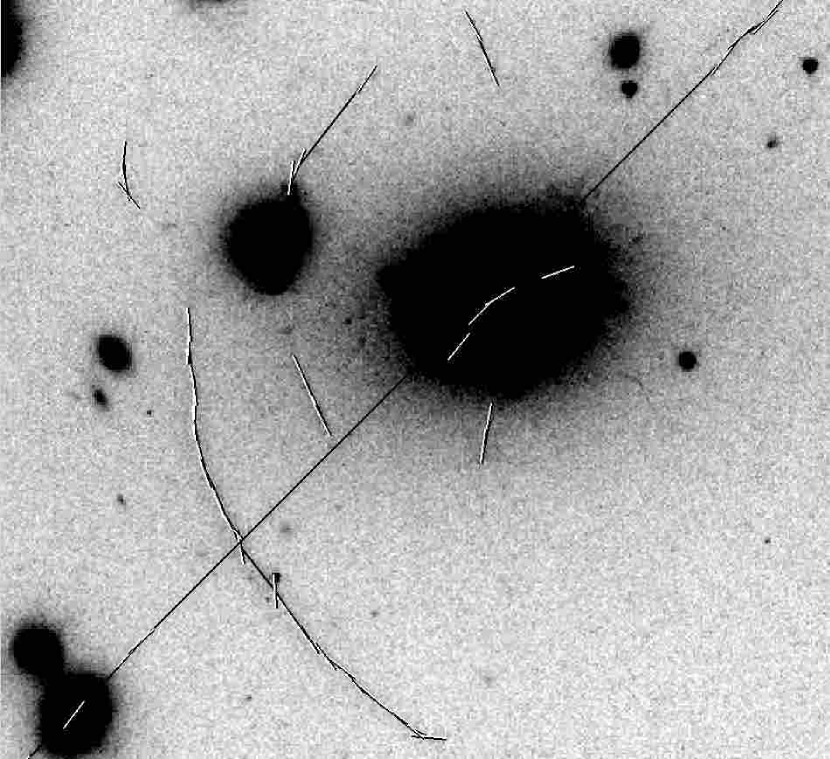
To connect the nodes, the relative distance $\@vec{\Delta}$ from a node $i$ to every other node $j$ is calculated using Eq. (8). From this, a modified distance

$$r_{e}=\sqrt{\Delta_{1}^{2}+16\Delta_{2}^{2}}$$ (16)

is computed for each node with $\left|\frac{\Delta_{2}}{\Delta_{1}}\right|$, i.e. within an angle of $\pi/4$. The nodes with the lowest $r_{e}$ among all nodes are connected to node $i$, if they exist.

The angle $\pi/4$ limits the curvature to less than $\pi/4d_{1}$. The metric $r_{e}$ assigns equal distances from cell $i$ to all points on an ellipse with an axis ratio of four and a major axis parallel to the $e_{1}$ axis centered on $i$. Consequently, nodes with a small perpendicular distance are connected preferentially. This reduces the influence due to nodes of features crossing within the same object.

The implementation of this method can lead to a disconnected graph, with individual features separated by independent structures in the object. A connected graph can be created by repeatedly connecting the subgraph containing the first node in the object to the closest subgraph separated from it. Specifically, an additional variable $v$ is assigned to each node, which is initially set to zero for all nodes. In a loop, the value one is recursively propagated to all connected nodes, starting in node zero. In the next step, the distance $r_{e}$ is measured between all nodes $i$ connected with node zero which thus have $v^{i}=1$, and all disconnected nodes $j$ with $v^{j}=0$. The pair of nodes $i$ and $j$ with the minimal distance is then connected, all $v$ are re-initialised with zero, and the process is repeated until no disconnected nodes are left.

2.5.2 Generation of subgraphs from graphs

The graphs resulting from the preceding procedure are not ideally suited for post-processing because they may belong to multiple features, or features contaminated by spurious structures. Therefore, all their subgraphs which possibly represent either part of or a complete valid feature are generated using the specific structure of the graphs representing valid features: each node must be connected to either one or two other nodes, and the relative angle between two edges at a node must fall within $\pi\pm\alpha$, with $0\leq\alpha\lesssim\pi/4$ depending on the maximum allowed curvature. That is, graphs satisfying this definition are either arc-like, with two end nodes having only one connection and an arbitrary number of nodes with two edges in between, or ring-like, having no end nodes and containing only nodes met by two edges.

To find the first variant, all edges connected to a node $i$ are checked for edges joining on the opposite side of the node within the specified angle range. If there is no such opposite edge, node $i$ is a starting or ending point, and the algorithm recursively goes through all nodes connected through this and the following edges which are within the required angle interval with their preceding edges, and lead to nodes not already belonging to the current path. All nodes $j$ in this recursive scheme for which no successive edge is found within the angle interval are end nodes. A new graph is created starting with the path from $i$ to $j$ if an equal graph, consisting either of the same path from $i$ to $j$ or its exact reverse, does not exist yet.

To find the second variant, one can start the recursion for all edges in the original graph which are not yet part of any other graph. The resulting graphs will miss one edge and thus have a starting and an ending point, which makes further computations slightly easier, but will equally represent any underlying feature. We tested our algorithm setting $\alpha=\pi/5$.

2.5.3 Graph concatenation

Our algorithm’s final step is the concatenation of those new graphs which may represent a single feature. To this end, a circle is fit to each graph, and the nearest of any other graphs falling on that circle is added to it, provided it is closer than three times the angle spanned by the two lines from the centre of the circle to the first and last nodes in the original graph.

Then, a new circle is fit to restart the procedure. Since a true least-squares fit of a circle to a set of points is impossible analytically, and finding the solution numerically is computationally expensive, the fit is simplified by assuming that one of the first and the last two nodes of the graph fall exactly on the circle. The radius can then be fit analytically, and the best fit in a least-square sense is chosen from the four solutions. The deviation of this method from an unconstrained fit is negligible in most cases, although the method is feasible only because of the already simple form of the given graphs.

3 Potential problems

A number of unresolved problems remain, as well as problems with known solutions. Both are considered in the following.

3.1 Ellipticity bias

Given an odd scale size $d_{0}$, the straightforward method of measuring ellipticities for each cell computes the sum

$$Q_{ij}=\frac{\sum_{\@vec{x}\in A}(x_{i}-\bar{x}_{i})(x_{j}-\bar{x}_{j})q(I(\@vec{x}))}{\sum_{\@vec{x}\in A}q(I(\@vec{x}))}\;,$$ (17)

inside the rectangle

$$A=\left\{\@vec{x}\in\mathbb{Z}^{2}:x^{\rm{min}}_{1}\leq x_{1}<x^{\rm{max}}_{1}\wedge x^{\rm{min}}_{2}\leq x_{2}<x^{\rm{max}}_{2}\right\}$$ (18)

$$\begin{aligned} &\mbox{with}&&\@vec{x}^{\rm{min}}=\left(\bar{x}_{1}-\frac{d_{0}-1}{2},\bar{x}_{2}-\frac{d_{0}-1}{2}\right)\\ &\mbox{and}&&\@vec{x}^{\rm{max}}=\left(x^{\rm{min}}_{1}+d_{0},x^{\rm{min}}_{2}+d_{0}\right)\;,\end{aligned}$$

where $\@vec{\bar{x}}$ are pixel coordinates within the cell. However, since noise fluctuations in the four corners of $A$ have a stronger influence on the secondary brightness moments than similar fluctuations along the edges or in the interior of the cell, the resulting ellipticities will preferentially be aligned with the diagonal.

This significant ellipticity bias can be avoided using position-dependent weights $q^{\prime}(I(\@vec{x}),\@vec{x})=q(I(\@vec{x}))\cdot A_{p}(\@vec{x})$ and modified coordinate components $x^{\prime}_{1}(\@vec{x})$ and $x^{\prime}_{2}(\@vec{x})$ in (17), e.g.

$$Q_{ij}=\frac{\sum_{\@vec{x}\in A}(x^{\prime}_{i}-\bar{x}_{i})(x^{\prime}_{j}-\bar{x}_{j})q^{\prime}(I(\@vec{x})),\@vec{x})}{\sum_{\@vec{x}\in A}q^{\prime}(I(\@vec{x}),\@vec{x})}\;,$$ (19)

where $A_{p}(\@vec{x})$ is the area of overlap between a circle around $\@vec{\bar{x}}$ with radius $\frac{d_{0}}{2}$ and the horizontally aligned square of one pixel side length centred on and typically associated with a single pixel at position $\@vec{x}$. The centre of $A_{p}(\@vec{x})$ is $\@vec{x^{\prime}}(\@vec{x})$, and the total integration area $A$ is the same as above. Using only discrete centre coordinates $\@vec{\bar{x}}$, these values can be pre-calculated analytically during the initialisation of the algorithm (see Appendix C).

3.2 Influence of point sources and galaxies

Several problems are mostly associated with point sources in the astronomical context, although they can also appear in other applications.

For a single bright point source, one problem already solved by setting a minimal object length is the creation of objects from multiple cells converging to the exact same location. An efficient method to approximate the length of an object represented by a set of cells is to first find the cell $j$ farthest from an arbitrary cell $i$, and then the cell $k$ farthest from cell $j$, using the distance of cell $k$ from cell $j$ as a length measurement. This is not necessarily the largest pairwise distance in the object, but it can only be smaller by a factor of $\sqrt{3}$ (see Appendix B).

A closely related problem for very bright point sources is caused by brightness slopes which may be much more extended than the scale size $d_{0}$. Since a fixed number of iterations is used to determine the nearest local centre-of-brightness, cells do not necessarily complete the path to this point and measure the secondary brightness moments on the slope. They will then have orientations parallel to the slope’s gradient and can, depending on the original cell position, generate spurious detections. This can be avoided by setting limits for the total spatial displacement of a cell and discarding cells outside from further computations. Using $q(I)=\mathrm{max}(I-\bar{I},0)$ and assuming a constant slope, the total spatial displacement is the number of iterations times $d_{0}/3$, and less for local brightness maxima with their negative curvature in the brightness profile. We set the limit to $8d_{0}/11$ for testing the algorithm. A welcome side effect of this approach is the preservation of the valid cells’ original neighbourhoods.

As a consequence of averaging over an area characterised by the scale size, bright pixels in the vicinity of a valid feature can outshine it and prevent its detection. Since point-source images must be closer to a feature than about half the scale size $d_{0}$ to pull cells away from it during the centre-of-brightness determination or to influence the ellipticity measurement, choosing a smaller value for $d_{0}$ can avoid this problem at the cost of a lower signal-to-noise ratio.

Clustered point sources can create false detections by imitating substructures of a valid feature. Since the distinction of substructure from point-source clustering is impossible after averaging over $d_{0}$, which is one of the basic ideas behind the algorithm, post-processing of the brightness profiles underlying each object graph is possibly the only way of solving this type of problem. Even a single point source enhances the likelihood for a spurious detection by pulling multiple cells towards a single location, thereby compromising the simple cell-count filter.

Adding a single cell $j$ with sufficient correlations $c^{j}$ and $C^{ij}$ further away than the minimal object length and in the neighbourhood of any cell $i$ among the already assembled cells results in a detection. For farther cells with high spatial correlation, i.e. placed along the assembled cells’ mean direction, the orientational correlation will also be increased if they are affected by the point-source image, causing them to point at the source.

The situation is similar for two point sources, which can create false detections if their distance in the image exceeds the minimal object length and if a cell located at the centre of each point source image can “see” the image of the other within its averaging area. Of course, a larger point-spread function increases the influence of the points sources.

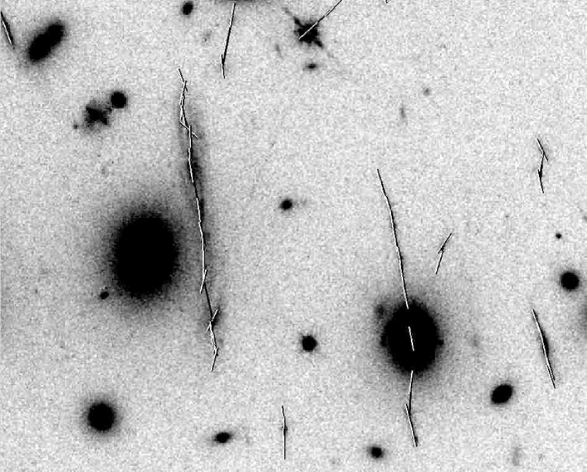
Searching for arcs, extended diffraction spikes and blooming satisfy all criteria for valid features and will thus cause spurious detections. One approach to avoiding them is to determine the location of diffraction spikes in an independent step by searching for bright point sources, then masking blooming by its maximal brightness and approximating the extended point-spread function. If an arc candidate is found which spatially coincides with a diffraction spike, it can then be flagged or invalidated.

Searching for prominent arcs, the scale size may be too large for detecting galaxies, but if the scale size is small enough, they will also cause spurious detections if they fulfil the criteria for valid features. They can then be eliminated based on their lower length and length-to-width ratio of their isophotes. Another possible way to invalidate them is to compute their radial brightness profiles, which will generally be shallower for gravitationally lensed objects. If small arcs are included into the search, however, it may be impossible to reliably remove them unless observations in multiple frequency bands allow a colour discrimination.

3.3 Chip and image boundaries

When image data from CCDs of different resolution and sensitivity are combined into one image, e.g. for the HST/WFPC2 instrument, or if the image examined is a mosaic, boundaries across the image between regions of different noise level or mean background intensity may occur. A noticeable change in the mean background intensity shifts cells by about $d_{0}/2$ towards the brighter region, significantly increasing the cell density in this narrow space and possibly creating an orientation bias perpendicular to the boundary. Since both directional correlation and a low spatial distance perpendicular to each cell’s direction are required for the creation of objects, this case will not necessarily result in spurious detections, although they will become more likely due to the increase in cell density.

A change in the noise level and similar mean background intensities in both regions typically only introduces an ellipticity bias in the direction of the boundary, thereby enhancing the directional correlation. Using a weight function $q(I)=\mathrm{max}(I-\bar{I},0)$ for the determination of the centre-of-brightness which ignores pixels with intensities below $\bar{I}$ additionally leads to a cell shift into the region of higher noise and an increase in cell density. For these reasons, regions of different noise in a single image may cause spurious detections. Setting $q(I)=0$ for pixels outside the image can be seen as a boundary between regions of equal background but with a noise change equal to the noise in the image. In the current implementation of our algorithm, false detections at the image boundaries are avoided by simply invalidating cells straddling them. Another approach could generate noise outside the image, with the drawback of decreasing the signal-to-noise ratio for the affected cells.

3.4 Noise and background gradient

We measure the sensitivity of the algorithm using a model image of $1000\times 1000$ pixels with intensities drawn from a Poisson distribution. The signal is a smoothed line segment of a quarter circle with 500 pixels radius, randomly oriented and shifted by at most 50 pixels from the image centre. Intensities without noise are given by $I(\@vec{x})=I_{0}+I_{\mathrm{s}}\exp\left(-d^{2}(\@vec{x})/2\sigma^{2}\right)$, where $I_{0}$ is the background intensity, $I_{\mathrm{s}}$ is the peak signal intensity along the ridge of the line segment, $d(\@vec{x})$ is the distance of the pixel at $\@vec{x}$ from the line segment and $\sigma$ is a smoothing scale. The actual intensities in the image are Poisson distributed random numbers with a mean of $I(\@vec{x})$ and standard deviation of $\sqrt{I(\@vec{x})}$.

Although the resulting model signal is not identical to a line segment with intensity $\sqrt{2\pi}\sigma I_{\mathrm{s}}$ above the background smoothed with a Gaussian kernel, it is a good approximation, easily constructed for comparison with other algorithms and equally close to the typical valid feature in astronomical applications as a line segment smoothed with a Gaussian.

For each set of parameters, we note both the number of valid detections $N_{\mathrm{valid}}$, zero or one, and the number of spurious detections $N_{\mathrm{spurious}}$, where a detection was counted as valid if all nodes in the detected graph were inside a maximum distance of one $\sigma$ from the arc and the graph was at least 196 pixels long, one fourth of the line segment’s length. If more than one detection fulfilled this criterion, only the first was counted.

For a constant background of $I_{0}=100$, a central signal intensity of $I_{\mathrm{s}}=6$ and $\sigma=10$, the mean number of spurious detections in ten runs for various scaling sizes is given in Table 1, showing the detection of short, random structures in the background. For the range of scale sizes shown, the number of valid detections was zero.

Table 1: Dependence of spurious detections on the scale size.

$d_{0}$	5	7	9	11	13	15	17	19
$N_{\rm{spr}}$	385.5	27.9	1.1	4.8	0.5	0.3	0.1	0

For the same values $I_{0}$ and $I_{\mathrm{s}}$, the average detection ratio $N_{\mathrm{valid}}/(1+N_{\mathrm{spurious}})$ found in ten runs is plotted as a function of the scale size $d_{0}$ for $\sigma=6,8,10,12$ in Figure 5. For scale sizes below $2\sigma$, the cell’s areas are dominated by noise even close to the feature, preventing its detection, and for scale sizes above $10\sigma$, the feature cannot attract enough cells to sufficiently increase the first correlation value $c^{i}$. While there are detections on the line segment for large scale sizes, these are too short to be valid. With increasing $\sigma$, the integrated signal intensity increases proportionally, improving the likelihood for detection, as evidenced by the larger range of scale sizes with $N_{\mathrm{valid}}=1$.

Figure 5: The normalised number of valid detections, $N_{\mathrm{valid}}/(1+N_{\mathrm{spurious}})$, is displayed as a function of the scale size $d_{0}$ for different smoothing scales $\sigma$.

For $I_{0}=100$, $\sigma=10$ and the scale size $d_{0}=45$ best adapted to this $\sigma$, the average detection ratio $N_{\mathrm{valid}}/(1+N_{\mathrm{spurious}})$ in 50 runs for different signal intensities $I_{\mathrm{s}}$ is given in Table 2.

Table 2: Detection ratio for $I_{0}=100$, $\sigma=10$ and $d_{0}=45$ depending on the central signal intensity $I_{\mathrm{s}}$.

$I_{\mathrm{s}}$	4.2	4.4	4.6	4.8	5.0	5.2	5.4	5.6
$\frac{N_{\mathrm{valid}}}{1+N_{\mathrm{spurious}}}$	0	0.03	0.12	0.38	0.42	0.63	0.89	1

In both tests, a noisy but on average constant background was assumed. If the background has a slope steeper than the intensity slope up to the ridge line for a background-subtracted feature, cells cannot find this feature’s location during the determination of their centre-of-brightness, prohibiting detection. In astronomical observations, bright foreground objects can induce steep intensity slopes which are generally not well described by a first-order approximation of the local background, thus offering a challenge to possible background-subtraction methods.

4 Implementation specifics

During the implementation of the above ideas, several arbitrary choices were made, some of them with a bearing on the results below in 5, others in an effort to make the code more efficient, and some to keep the source code manageable.

4.1 Initial cell placement

The most important free parameter, and ideally the only one to be changed for different image data, is the scale size $d_{0}$. Based on it, cells are initially placed on a regular rectangular grid spaced by $d_{1}=d_{0}/2$. Determining the closest centre-of-brightness is done by applying a discretised version of Eq. (1) to find $\bar{\@vec{x}}$ in a rectangular area $A$ as defined in (18) for each of three iterations. Using a rectangular area and thereby allowing farther spatial shifts in the diagonal direction instead of a circular disk for this part of the algorithm compensates for the initially larger diagonal distance of the cells.

4.2 Classes and local indices

Since the source code was written in C++, it was convenient to use structures and classes to represent cells, objects and graphs, providing easy access to data members and hiding most of the necessary memory management and initialisations from the primary functions. Since the number of cells remains constant while the algorithm proceeds, it was sufficient to implement them as one-dimensional arrays of cell structures, where the original position and neighbourhood can be readily derived from each cell’s index. Graphs are described by classes for nodes, single graphs, and the list containing all graphs. To increase the efficiency of the graph concatenation, whose complexity is $\mathcal{O}(n^{2})$ in the number of graphs $n$, the graph list can be used to subdivide the image into rectangular regions, each of which maintains a list of all graphs with nodes in it. These lists can be initialised with linear complexity and are, combined with a method to mark already processed graphs, used to enumerate only those graphs in relevant areas. However, while significantly decreasing the execution time, this does not reduce the concatenation’s squared dependence on the number of graphs.

4.3 Performance

Applying the algorithm to a FITS image of $3021\times 3021$ pixels with single (floating point) precision using a scale size $d_{0}$ of 27 pixels and a very low minimal length of 22 pixels on a personal computer with one 2.80 GHz processor and 1 GB RAM took approximately $4.4\,\mathrm{s}$ total execution time of the calculation thread, and resulted in 137 detected objects prior to applying any later filters. Apart from setting a minimal object length and cell count, no further filters are included yet. Most of that time, namely $\sim 3.9\,\mathrm{s}$, was needed for the determination of the centres-of-brightness and the orientations. The graph concatenation needed $\sim 0.1\,\mathrm{s}$.

Changing the scale size to 13 pixels and reducing the minimal object length to 10 pixels resulted in 1033 mostly spurious detections of small features, and increased the execution time to $\sim 11.8\,\mathrm{s}$, of which the determination of the centres of brightness and orientations needed $\sim 5.6\,\mathrm{s}$ and the graph concatenation another $\sim 5.6\,\mathrm{s}$.

Applying the algorithm with the latter parameters to another single-precision FITS image with $8500\times 8300$ pixels and less small-scale structure gave 395 detections, many of which are diffraction spikes, and took $\sim 161.2\,\mathrm{s}$ in total, $99.9\,\mathrm{s}$ of which were used for the centre-of-brightness and orientation computations, and $\sim 3.5\,\mathrm{s}$ seconds for the graph concatenation. The remaining $\sim 57.7\,\mathrm{s}$ were used for transferring data between the threads and initialisation. Considering that the area is only $\sim 8.5$ times larger, the increase by a factor of $\sim 25.6$ in execution time for the algorithm’s first step is mostly caused by extensive memory swapping, as is the steep increase in the time needed for the data transfer and initialisations. Apart from conventional optimisation or using more RAM, this can easily be solved by applying the algorithm several times on distinct overlapping subregions in the image.

5 Results

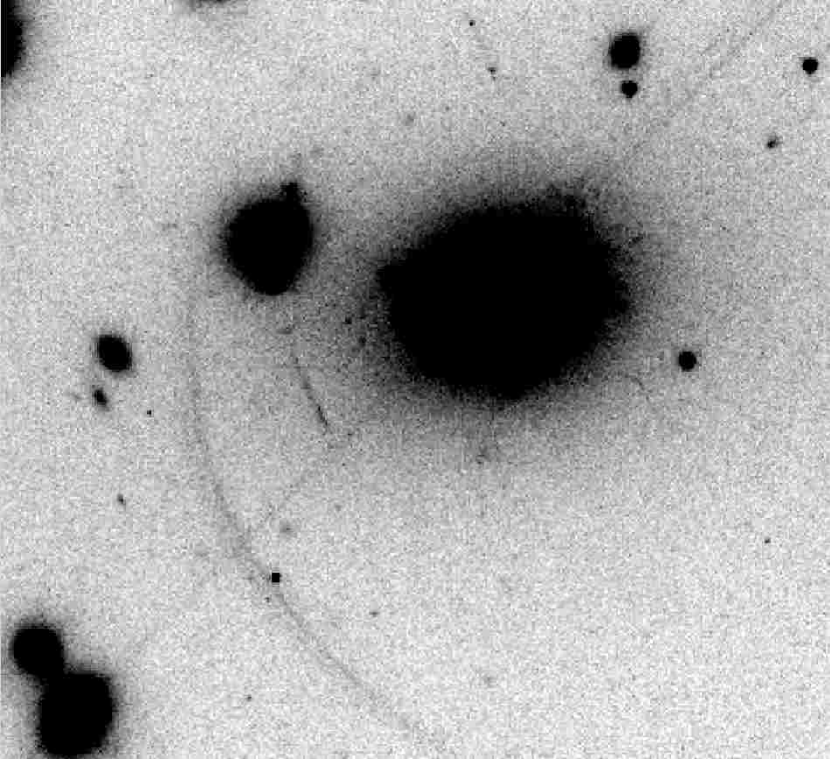
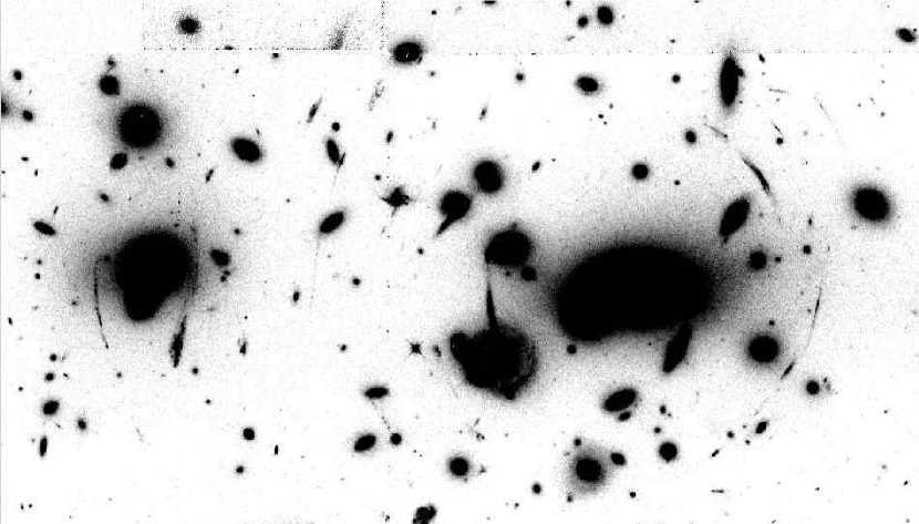
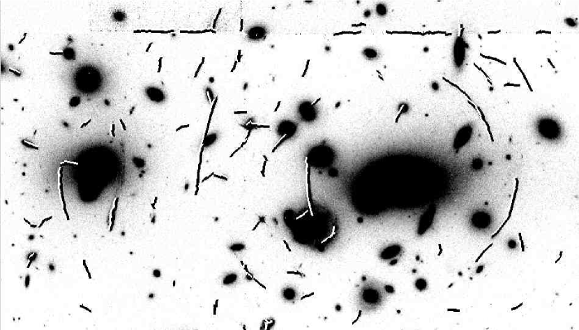
We developed our algorithm primarily using an HST/WFPC2 observation of Abell 2390 with an exposure time of $2100\,\mathrm{s}$ in the F814W filter as the base image, which includes multiple arcs. We also tested the algorithm against other images to confirm its generalisability.

Figure 6: This section of the image was used to “train” the algorithm. It is shown here without additional markers.

Figure 7: The structured arc in the same image is shown with graphs overlaying the detections. The scale size is $d_{0}=27$ here and in all of the other HST images shown.

Figure 8: Another WFPC2 observation of Abell 2218, taken with a 702 nm filter and an exposure time of $1900\,\mathrm{s}$.

Figure 9: This image shows detections marked by black and white lines obtained with a scale size of $d_{0}=25$. Prominent spurious detections can be seen near the horizontal border between the WFPC2 CCDs.

6 Future work

Though it is one aim of the presented algorithm to introduce as few as possible arbitrary methods and variables, several exist, and they should be optimised. This refers to the free parameters already introduced in the text, but also general methods. For example, one possibility would be to change the initially rectangular grid to a hexagonal one to provide an equally spaced set of immediate neighbours and possibly a reduction in necessary overlap.

Point sources can, as detailed in 3.2, significantly increase the likelihood of spurious detections, which are probably best removed by a post-processing of those areas in the image underlying detected graphs. Since these areas represent only a fraction of the complete image, more elaborate filtering techniques are possible, but as of now, a filter capable of distinguishing arc substructure from clustered point sources was not implemented yet. Stellar photometry in crowded fields already deals with similar issues, and trying to model a feature as a superposition of point-spread functions, similar to the approach of the daophot program (Stetson (1987)), could be a sound if computationally expensive approach. Using the large elongation of valid features, the width of low-intensity isophotes could also be used to discriminate features induced by only one or two point sources, although a slope in the detection’s background increases the minimal isophote intensity, possibly rendering this method useless and necessitating careful background subtraction.

Diffraction spikes are another problem mentioned in 3.2, and a method to estimate their positions without specific a priori information on the detector is already implemented, but must be combined with the our algorithm to remove detections coinciding with them.

We presented a first quantification of the algorithm’s sensitivity and parameter dependence in 3.4, but the simple way of modelling a valid feature and the assumption of a constant background intensity make it difficult or impossible to extrapolate to the applicability of the algorithm on real datasets from this. Also, the observational data presented above was less than comprehensive, since comparatively high-quality images were used. For these reasons, the algorithm will be applied to simulated strong-lensing images with varying seeing conditions and detector properties as well as to data available from current surveys, e.g. the HST-based COSMOS or ground-based observations which, given their wider area, are particularly interesting.

As of now, the algorithm uses only images taken in one spectral filter. However, where sufficiently deep and resolved observations are available in several spectral bands, this information could be used both to remove spurious detections separable by the varying spectra of their components and to increase the algorithm’s sensitivity by using the additional parameter space for correlation measurements.

7 Summary

We have presented an algorithm for the fast and automatic detection of arc-like features in astronomical data. The algorithm proceeds in three major steps. First, the image pixels are grouped into square cells which are moved in a fixed number of iteration steps towards their centre of brightness. They thus find a final position on or near a local intensity peak. Second, the quadrupole moment of the light distribution is measured in each cell, where it defines an elongation and a direction. Third, the neighbourhood of each cell is searched for such cells whose intensity distribution points into a similar direction. If so, the cells are connected to form an object, and the procedure is continued until all cells have been processed. The objects found in this way can then be automatically classified.

Having arc-like features in mind which may be just above the noise limit, we avoid smoothing in the algorithm which may give rise to subtle biases. Smoothing may make arcs disappear, but it may also create spurious arc-like features by anisotropic stretching of positive noise fluctuations. The algorithm also avoids object detection and uses only the local intensity distribution in the cells. These design criteria enable an implementation which operates very fast. For example, it was possible to scan an image of $3021\times 3021$ pixels in less than five seconds on an ordinary desktop PC.

We used HST images to illustrate the steps of the algorithm and its efficiency. Remaining potential problems concern the presence of bright point sources and extended galaxies in the images, boundaries of images and CCD chips in image mosaics, and residual gradients in the noise or the image backgrounds, and we outline how they can be overcome.

Apart from several parameters which control how cells may be connected with neighbouring cells to form objects, the single main parameter is the number of pixels to be grouped into a cell. This can be suitably chosen depending on the resolution and the quality of the image, and the algorithm is fast enough to allow calibration runs.

The main application which we have in mind for the algorithm is blindly scanning wide-field images for arcs in order to construct unbiased arc samples from large data sets. We shall study in a forthcoming paper how the detection efficiency and reliability will depend on noise, seeing, and the density of foreground objects.

Appendix A Obtaining an orientation from the complex ellipticity $\chi$

Figure 10: An elliptical isophote and the geometric construction of the orientation $\vartheta$.

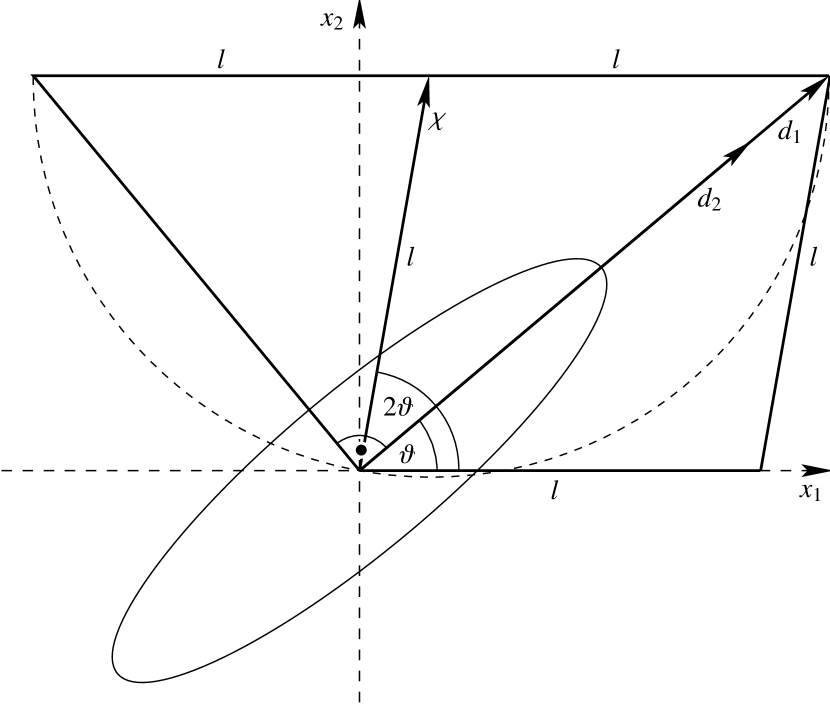
In $\mathds{C}$, the real axis and the complex ellipticity $\chi=\frac{1-r^{2}}{1+r^{2}}\exp(2\mathrm{i}\vartheta)$ span $2\vartheta$, twice the angle $\vartheta$ in image space between the $x_{1}$-axis and the main axis of an underlying ellipse. Writing $(\chi_{1},\chi_{2})=(\Re(\chi),\Im(\chi))$, a vector parallel to the ellipse’s main axis can be obtained as $\@vec{d_{1}}=(\chi_{1}+|\chi|,\chi_{2})$, one diagonal of the rhombus with sidelength $l=|\chi|$ seen on the right side of Figure 10. The angle between $\@vec{d_{1}}$ and the $x_{1}$-axis is $\vartheta$. Since $|\@vec{d_{1}}|\rightarrow 0$ for $2\vartheta\rightarrow\pi$, this method cannot be used for the bisection of angles $2\vartheta$ close to $\pi$. Of course, one can also bisect $2\vartheta$ using $\@vec{d_{2}}=(\chi_{2},|\chi|-\chi_{1})$, i.e. the vector $(\chi_{1}-|\chi|,\chi_{2})$ rotated clockwise by $\frac{\pi}{2}$, where Thales’ theorem using the semicircle in Figure 10 can be used to show that the angle between $(\chi_{1}-|\chi|,\chi_{2})$ and $\@vec{d_{1}}$ must be $\frac{\pi}{2}$. Contrary to $|\@vec{d}|$, $|\@vec{d_{2}}|\rightarrow 0$ for $2\vartheta\rightarrow 0$. Using

$$\@vec{d}=\begin{cases}(\chi_{1}+|\chi|,\chi_{2})&\mbox{for}\quad\chi_{1}\geq 0\\ (\chi_{2},|\chi|-\chi_{1})&\mbox{for}\quad\chi_{1}<0\\ \end{cases}$$

as in (4), $|\@vec{d}|\geq\sqrt{2}|\chi|$ in all cases, making a reliable computation of the orientation $\@vec{e}=\frac{\@vec{d}}{|\@vec{d}|}$ possible.

Appendix B $\sqrt{3}$ relation of the object length and the maximum pairwise distance

In 3.2, the following method is used to determine an approximate object length: First, an arbitrary cell $A\in\mathcal{M}$, where $\mathcal{M}$ is the set of all cells in the object, is choosen. Then, the cell $B\in\mathcal{M}$ farthest from $A$ is found. Last, the cell $C\in\mathcal{M}$ farthest from $B$ is determined where $r=|BC|$ is used as the object length. It can be shown that $\sqrt{3}r$ is greater or equal to the maximum pairwise distance for all cells in the object:

Figure 11: The length determination method used in 3.2 requires that the centre coordinates of all cells in the object must be in the intersection of the circular disks $\mathcal{A}$ and $\mathcal{B}$. It is shown that $\sqrt{3}r$ is greater or equal to the maximum pairwise distance of the cells in the object, which must be lesser or equal then $d$ if $r$ is between $|AB|$ (left dashed lines) and $\sqrt{2}|AB|$ (right dashed lines). For $r>\sqrt{2}|AB|$ the maximum pairwise distance is limited by $2|AB|$.

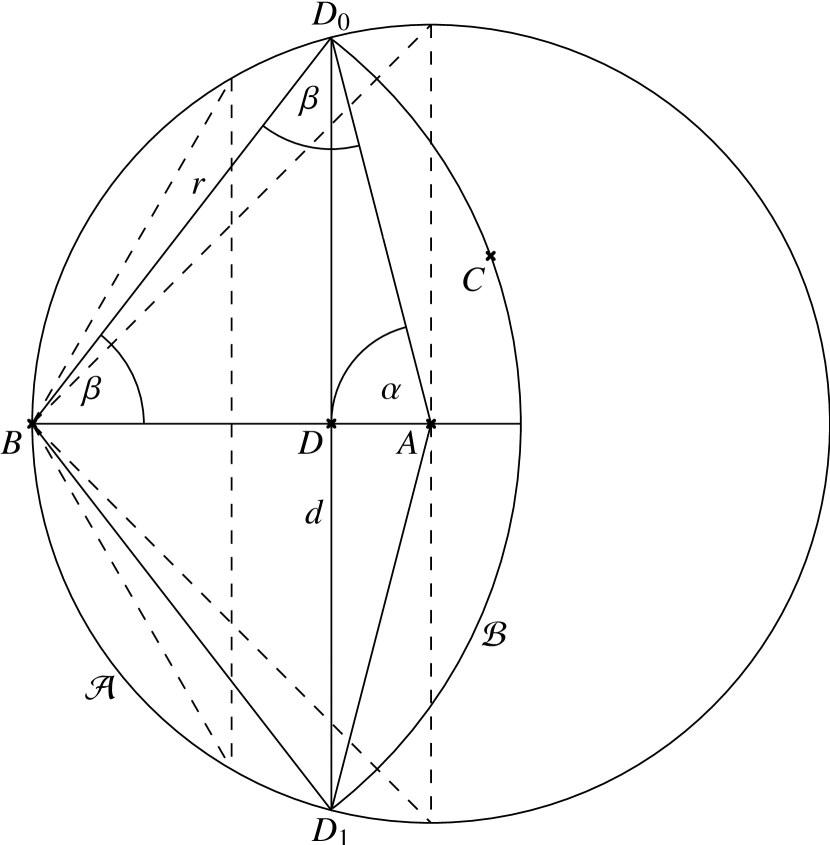
Putting the method in more formal terms,

$$A,B\in\mathcal{M} |AB|\geq|AX|\quad\forall X\in\mathcal{M}\quad\mbox{and}$$ with (20)

$$B,C\in\mathcal{M} |BC|\geq|BX|\quad\forall X\in\mathcal{M}$$ with (21)

$$\Rightarrow\; |BC|\geq|AB| |BC|\leq|BA|+|AC|\leq 2|AB|.$$ and (22)

From (20) and (21), all points in $\mathcal{M}$ are inside the intersection of the circular disk $\mathcal{A}$ around $A$ with radius $|AB|$ and the circular disk $\mathcal{B}$ around $B$ with radius $r=|BC|$. The point where the line between the intersections $D_{0}$ and $D_{1}$ of the boundaries $\partial\mathcal{A}$ and $\partial\mathcal{B}$ crosses the straight line $AB$ shall be $D$ and the distance between $D_{0}$ and $D_{1}$ shall be $d$, as illustrated in Figure 11. Using (22), the problem can be separated into three cases:

1. $r=|AB|$: $\mathcal{A}$ and $\mathcal{B}$ have equal radius, therefore the problem is symmetric and $|BD|=\frac{r}{2}$. From this, $(\frac{d}{2})^{2}=r^{2}-|BD|^{2}=r^{2}-(\frac{r}{2})^{2}\Rightarrow d=\sqrt{3}r$. Since $\frac{d}{2}>|BD|=|AD|$ and the circle with radius $\frac{d}{2}$ centred on $D$ therefore contains the complete intersection of $\mathcal{A}$ and $\mathcal{B}$, the maximum pairwise distance must be lesser or equal than $d$ and $\sqrt{3}r$ must be greater or equal than the maximum pairwise distance.
   

2. $|AB|<r\leq\sqrt{2}|AB|$: $\alpha=\angle{D_{0}AB}$ and $\beta=\angle{ABD_{0}}=\angle{BD_{0}A}$ as displayed in Figure 11. For $r>|AB|$ follows $\alpha>\frac{\pi}{3}$ and therefore $\beta<\frac{\pi}{3}$. Using this, $\cos\beta>\frac{1}{2}$ and $\left(\frac{d}{2}\right)^{2}=r^{2}-|BD|^{2}=r^{2}-r^{2}\cos^{2}\beta<\frac{3}{4}r^{2}\Rightarrow d<\sqrt{3}r$. For example using $|BD|=|AB|(1-\cos\alpha)$ and $\frac{d}{2}=|AB|\sin\alpha$ it is easily shown that $\frac{d}{2}\geq|BD|>|AD|$ and $d$ must again be greater or equal to the maximum pairwise distance. Consequently, $\sqrt{3}r$ is greater then the maximum pairwise distance.
   

3. $\sqrt{2}|AB|<r\leq 2|AB|$: the intersection between the circular disks $\mathcal{A}$ and $\mathcal{B}$ is equal to $\mathcal{A}$, therefore the maximum pairwise distance must be lesser or equal to $2|AB|<\sqrt{2}r<\sqrt{3}r$.

Appendix C Determination of the pixel/disk overlap area $A_{p}(\@vec{x})$ and centre $\@vec{x^{\prime}}(\@vec{x})$

Figure 12: Overlap of pixel areas with the area of a circular disk. The coordinates $(x,y)$ are chosen so that the disk’s centre is at their origin and the relevant pixel appears in the upper quadrant enclosed by the diagonal lines. To better illustrate the darker areas relevant to the integrals (C) to (C), an even diameter of four pixels was chosen; in the algorithm, an odd diameter equal to the scale size $d_{0}$ is used.

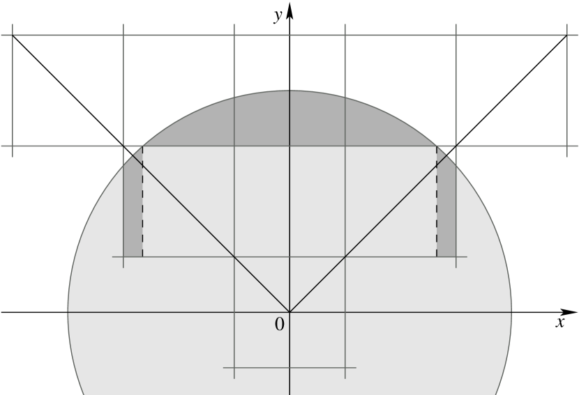
In 3.1 the intersection $A_{p}(\@vec{x})$ of a circular disk with radius $\frac{d_{0}}{2}$ around $\@vec{\bar{x}}$ and the square of one pixel sidelength representing a pixel at position $\@vec{x}$ must be computed as well as the centre $\@vec{x^{\prime}}(\@vec{x})$ of this intersection. With a circle radius of $R$, pixel coordinates $(x,y)$ chosen such that the circle’s centre is at $(0,0)$, $y\geq 0$ and $|x|\leq|y|$, and $A$ being the area inside the pixel square, the problem mostly reduces to the following integrals after some straightforward case distinctions:

$$\iint_{A}\mathrm{d}x\mathrm{d}y = \int_{x_{0}}^{x_{1}}\sqrt{R^{2}-x^{2}}-y_{0}\,\mathrm{d}x$$

$$= \left.\frac{1}{2}\left(x\sqrt{R^{2}-x^{2}}+R^{2}\mathrm{arctan}\left(\frac{x_{1}}{\sqrt{R^{2}-x^{2}}}\right)\right)-xy_{0}\right|_{x_{0}}^{x_{1}}$$

for computing parts of the area $A_{p}$, and

$$\iint_{A}\,x\mathrm{d}x\mathrm{d}y = \int_{x_{0}}^{x_{1}}x\left(\sqrt{R^{2}-x^{2}}-y_{0}\right)\mathrm{d}x$$

$$= \left.-\frac{1}{3}(R^{2}-x^{2})^{3/2}-\frac{x^{2}y_{0}}{2}\right|_{x_{0}}^{x_{1}}$$

as well as

$$\iint_{A}\,y\mathrm{d}x\mathrm{d}y = \int_{x_{0}}^{x_{1}}\int_{y_{0}}^{\sqrt{R^{2}-x^{2}}}y\,\mathrm{d}x\mathrm{d}y$$

$$= \int_{x_{0}}^{x_{1}}\frac{1}{2}(R^{2}-x^{2}-y_{0}^{2})\mathrm{d}x=\left.\frac{1}{2}x(R^{2}-y_{0}^{2})-\frac{1}{6}x^{3}\right|_{x_{0}}^{x_{1}}$$

for finding the centre $\@vec{x}^{\prime}$. The remaining area integrals have fixed limits of the form $\iint_{A}\mathrm{d}x\mathrm{d}y=\int_{x_{0}}^{x_{1}}\int_{y_{0}}^{y_{1}}\mathrm{d}x\mathrm{d}y$ and can be included in a straightforward manner.

References

- Alard (2006) Alard, C. 2006, ArXiv Astrophysics e-prints astro-ph/0606757
- Horesh et al. (2005) Horesh, A., Ofek, E. O., Maoz, D., et al. 2005, ApJ, 633, 768
- Lenzen et al. (2004) Lenzen, F., Schindler, S., & Scherzer, O. 2004, A&A, 416, 391
- Stetson (1987) Stetson, P. B. 1987, PASP, 99, 191