Non-Gaussian Covariance of CMB $B$-modes of Polarization and Parameter Degradation

Abstract

The $B$-mode polarization lensing signal is a useful probe of the neutrino mass and to a lesser extent the dark energy equation of state as the signal depends on the integrated mass power spectrum between us and the last scattering surface. This lensing $B$-mode signal, however, is non-Gaussian and the resulting non-Gaussian covariance to the power spectrum cannot be ignored as correlations between $B$-mode bins are at a level of 0.1. For temperature and $E$-mode polarization power spectra, the non-Gasussian covariance is not significant, where we find correlations at the $10^{-5}$ level even for adjacent bins. The resulting degradation on neutrino mass and dark energy equation of state is about a factor of 2 to 3 when compared to the case where statistics are simply considered to be Gaussian. We also discuss parameter uncertainties achievable in upcoming experiments and show that at a given angular resolution for polarization observations, increasing the sensitivity beyond a certain noise value does not lead to an improved measurement of the neutrino mass and dark energy equation of state with $B$-mode power spectrum. For Planck, the resulting constraints on the sum of the neutrino masses is $\sigma_{\Sigma m_{\nu}}\sim 0.2\ \mathrm{eV}$ and on the dark energy equation of state parameter we find, $\sigma_{w}\sim 0.5$.

I Introduction

The applications of cosmic microwave background (CMB) anisotropy measurements are well known Kno95 ; its ability to constrain most, or certain combinations of, parameters that define the currently favorable cold dark matter cosmologies with a cosmological constant is well demonstrated with anisotropy data from Wilkinson Microwave Anisotropy Probe Sper06 . Furthermore the advent of high sensitivity CMB polarization experiments with increasing sensitivity keating suggests that we will soon detect the small amplitude $B$-mode polarization signal. While at degree scales one expects a unique $B$-mode polarization signal due to primordial gravitational waves KamKosSte97 , at arcminute angular scales the dominant signal will be related to cosmic shear conversion of $E$-modes to $B$-modes by the large-scale structure during the photon propagation from the last scattering surface to the observer today Zaldarriaga:1998ar .

This weak lensing of cosmic microwave background (CMB) polarization by intervening mass fluctuations is now well studied in the literature lensing ; Hu00 , with a significant effort spent on improving the accuracy of analytical and numerical calculations (see, recent review in Ref. Cha ). As discussed in recent literature manoj , the lensing $B$-mode signal carries important cosmological information on the neutrino mass and possibly the dark energy, such as its equation of state manoj , as the lensing signal depends on the integrated mass power spectrum between us and the last scattering surface, weighted by the lensing kernel. The dark energy dependence involves the angular diameter distance projections while the effects related to a non-zero neutrino mass come from suppression of small scale power below the free-streaming scale.

Since the CMB lensing effect is inherently a non-linear process, the lensing corrections to CMB temperature and polarization are expected to be highly non-Gaussian. This non-Gaussianity at the four-point and higher levels are exploited when reconstructing the integrated mass field via a lensing analysis of CMB temperature and polarization HuOka02 . The four point correlations are of special interest since they also quantify the sample variance and covariance of two point correlation or power spectrum measurements Scoetal99 . A discussion of lensing covariance of the temperature anisotropy power spectrum is available in Ref. Coo02 . In the case of CMB polarization, the existence of a large sample variance for $B$-modes of polarization is already known smith , though the effect on cosmological parameter measurements is yet to be quantified. Various estimates on parameter measurements in the literature ignore the effect of non-Gaussianities and could have overestimated the use of CMB $B$-modes to tightly constrain parameters such as a neutrino mass or the dark energy equation of state. To properly understand the extent to which future polarization measurements can constrain these parameters, a proper understanding of non-Gaussian covariance is needed.

Here, we discuss the temperature and polarization covariances due to gravitational lensing. Initial calculations on this topic are available in Refs. smith ; smith2 , while detailed calculations on the CMB lensing trispectra are in Ref. Hu01 . Here, we focus mainly on the covariance and calculate them under the exact all-sky formulation; for flat-sky expressions of the trispectrum, we refer the reader to Ref. HuOka02 . We extend those calculations and also discuss the impact on cosmological parameter estimates. This paper is organized as follows: In §II, we introduce the basic ingredients for the present calculation and present covariances of temperature and polarization spectra. We discuss our results in §III and conclude with a summary in §IV.

II Calculational Method

The lensing of the CMB is a remapping of temperature and polarization anisotropies by gravitational angular deflections during the propagation. Since lensing leads to a redistribution of photons, the resulting effect appears only at second order Cha . In weak gravitational lensing, the deflection angle on the sky is given by the angular gradient of the lensing potential, $\delta(\hat{\mathbf{n}})=\nabla\phi(\hat{\mathbf{n}})$, which is itself a projection of the gravitational potential $\Phi$:

$$\phi(\bm{)} = -2\int_{0}^{r_{0}}dr\frac{d_{A}(r_{0}-r)}{d_{A}(r)d_{A}(r_{0})}\Phi(r,\hat{{\bf m}}r)\,,$$ (1)

where $r(z)$ is the comoving distance along the line of sight, $r_{0}$ is the comoving distance to the surface of last scattering, and $d_{A}(r)$ is the angular diameter distance. Taking the multipole moments, the power spectrum of lensing potentials is now given through

$$\left<\phi_{lm}^{*}\phi_{lm}\right>=\delta_{ll^{\prime}}\delta_{mm^{\prime}}C_{l}^{\phi}$$ (2)

as

$$C_{l}^{\phi}=\frac{2}{\pi}\int k^{2}\,dkP(k)I_{l}^{\rm len}(k)I_{l}^{\rm len}(k)\,,$$ (3)

where

$$I_{l}^{\rm len}(k) = \int_{0}^{r_{0}}drW^{\rm len}(k,r)j_{l}(kr)\,,$$

$$W^{\rm len}(k,r) = -3\Omega_{m}\left({H_{0}\over k}\right)^{2}F(r){d_{A}(r_{0}-r)\over d_{A}(r)d_{A}(r_{0})}\,,$$ (4)

where $F(r)=G(r)/a(r)$ and $G(r)$ is the growth factor, which describes the growth of large-scale density perturbations. In our calculations we will generate $C_{l}^{\phi\phi}$ based on a non-linear description of the matter power spectrum $P(k)$. In the next three subsections we briefly outline the power spectrum covariances under gravitational lensing for temperature and polarization $E$- and $B$-modes. In the numerical calculations described later, we take a fiducial flat-$\Lambda$CDM cosmological model with $\Omega_{b}=0.0418$, $\Omega_{m}=0.24$, $h=0.73$, $\tau=0.092$, $n_{s}=0.958$, $A(k_{0}=0.05\ \mathrm{Mpc}^{-1})=2.3\times 10^{-9}$, $m_{\nu}=0.05$ eV, and $w=-1$. This model is consistent with recent measurements from WMAP Sper06 .

II.1 Temperature anisotropy covariance

The trispectrum for the unlensed temperature can be written in terms of the multipole moments of the temperature $\theta_{lm}$ as Hu01

$$\langle\theta_{l_{1}m_{1}}\theta_{l_{2}m_{2}}\theta_{l_{3}m_{3}}\theta_{l_{4}m_{4}}\rangle = C_{l_{1}}^{\theta}C_{l_{4}}^{\theta}(-1)^{m_{1}+m_{4}}\delta_{l_{1}l_{3}}^{m_{1}-m_{3}}\delta_{l_{2}l_{4}}^{m_{2}-m_{4}}+C_{l_{1}}^{\theta}C_{l_{3}}^{\theta}(-1)^{m_{1}+m_{3}}\delta_{l_{1}l_{2}}^{m_{1}-m_{2}}\delta_{l_{3}l_{4}}^{m_{3}-m_{4}}$$ (5)

$$+ C_{l_{1}}^{\theta}C_{l_{2}}^{\theta}(-1)^{m_{1}+m_{2}}\delta_{l_{1}l_{4}}^{m_{1}-m_{4}}\delta_{l_{2}l_{3}}^{m_{2}-m_{3}}\,.$$

It is straight forward to derive the following expression for the multipole moment of lensed $\theta$ field as a perturbative equation related to the deflection angle Hu00 :

$$\tilde{\theta}_{lm}=\theta_{lm}+\sum_{l_{1}m_{1}l_{2}m_{2}}\phi_{l_{1}m_{1}}\theta_{l_{2}m_{2}}I_{ll_{1}l_{2}}^{mm_{1}m_{2}}+\frac{1}{2}\sum_{l_{1}m_{1}l_{2}m_{2}l_{3}m_{3}}\phi_{l_{1}m_{1}}\theta_{l_{2}m_{2}}\phi_{l_{3}m_{3}}^{*}J_{ll_{1}l_{2}l_{3}}^{mm_{1}m_{2}m_{3}}\,,$$ (6)

where the mode-coupling integrals between the temperature field and the deflection field, $I_{ll_{1}l_{2}}^{mm_{1}m_{2}}$ and $J_{ll_{1}l_{2}l_{3}}^{mm_{1}m_{2}m_{3}}$, are defined in Hu01 ; CooLi .

As for the covariance of the temperature anisotropy powerspectrum, we write

$$\text{Cov}_{\theta\theta}\equiv\frac{1}{2l_{1}+1}\frac{1}{2l_{2}+1}\sum_{m_{1}m_{2}}\langle\tilde{\theta}_{l_{1}m_{1}}\tilde{\theta}_{l_{1}m_{1}}^{*}\tilde{\theta}_{l_{2}m_{2}}\tilde{\theta}_{l_{2}m_{2}}^{*}\rangle-\tilde{C}_{l_{1}}^{\theta}\tilde{C}_{l_{2}}^{\theta}=\mathcal{O}+\mathcal{P}+(\mathcal{Q}+\mathcal{R})\delta_{l_{1}l_{2}}$$ (7)

where the individual terms are

$$\mathcal{O} = \frac{2}{(2l_{1}+1)(2l_{2}+1)}\sum_{L}{C_{L}^{\phi}}\left[(F_{l_{1}Ll_{2}}C_{l_{2}}^{\theta})^{2}+(F_{l_{2}Ll_{1}}C_{l_{1}}^{\theta})^{2}\right]$$

$$\mathcal{P} = \frac{4}{(2l_{1}+1)(2l_{2}+1)}\sum_{L}C_{L}^{\phi}C_{l_{1}}^{\theta}C_{l_{2}}^{\theta}F_{l_{1}Ll_{2}}F_{l_{2}Ll_{1}}$$

$$\mathcal{Q} = \frac{4}{(2l_{1}+1)^{2}}\sum_{L,l^{\prime}}{C_{L}^{\phi}}C_{l^{\prime}}^{\theta}C_{l_{1}}^{\theta}(F_{l_{1}Ll^{\prime}})^{2}$$

$$\mathcal{R} = -\frac{(l_{1}(l_{1}+1))}{2\pi(2l_{1}+1)}\sum_{L}C_{L}^{\phi}(C_{l_{1}}^{\theta})^{2}L(L+1)(2L+1)\,,$$ (8)

and the last two terms, which are related to the Gaussian variance, can be written in terms of the lensed temperature anisotropy power spectrum as

$$\mathcal{Q}+\mathcal{R}=\frac{2}{2l_{1}+1}(\tilde{C}_{l_{1}}^{\theta})^{2}\,,$$ (9)

where

$$\tilde{C}_{l}^{\theta} = [1-(l^{2}+l)R]C_{l}^{\theta}+\sum_{l_{1}l_{2}}C_{l_{1}}^{\phi}\frac{(F_{ll_{1}l_{2}})^{2}}{2l+1}C_{l_{2}}^{\theta}$$

$$R = \frac{1}{8\pi}\sum_{l_{1}}l_{1}(l_{1}+1)(2l_{1}+1)C_{l_{1}}^{\phi}$$

$$F_{ll_{1}l_{2}} = \frac{1}{2}[l_{1}(l_{1}+1)+l_{2}(l_{2}+1)-l(l+1)]\sqrt{\frac{(2l+1)(2l_{1}+1)(2l_{2}+1)}{4\pi}}\begin{pmatrix}l&l_{1}&l_{2}\\ 0&0&0\end{pmatrix}.$$ (10)

We note that Eqs. (10) are readily derivable when considering the lensing effect on the temperature anistropy spectrum as in Ref. Hu00 .

II.2 $E$-mode Polarization Covariance

Similar to the case with temperature, the trispectrum for an unlensed $E$-field can be written in terms of the multipole moments of the $E$-mode $E_{lm}$:

$$\langle E_{l_{1}m_{1}}E_{l_{2}m_{2}}E_{l_{3}m_{3}}E_{l_{4}m_{4}}\rangle = C_{l_{1}}^{E}C_{l_{4}}^{E}(-1)^{m_{1}+m_{4}}\delta_{l_{1}l_{3}}^{m_{1}-m_{3}}\delta_{l_{2}l_{4}}^{m_{2}-m_{4}}+C_{l_{1}}^{E}C_{l_{3}}^{E}(-1)^{m_{1}+m_{3}}\delta_{l_{1}l_{2}}^{m_{1}-m_{2}}\delta_{l_{3}l_{4}}^{m_{3}-m_{4}}$$ (11)

$$+ C_{l_{1}}^{E}C_{l_{2}}^{E}(-1)^{m_{1}+m_{2}}\delta_{l_{1}l_{4}}^{m_{1}-m_{4}}\delta_{l_{2}l_{3}}^{m_{2}-m_{3}}\,.$$

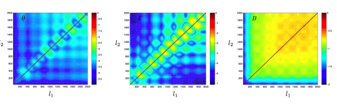
Figure 1: The correlation matrix [Eq. (25)] for temerature (left), $E$-mode (middle), and $B$-mode (right) power spectra between different $l$ values. The color axis is on a log scale and each scale is different for each panel. As is clear from this figure, the off diagonal correlation is weak for both $\theta$ and $E$-mode power spectra, but is more than $0.1$ for most entries for the $B$-mode power spectrum. This clearly shows that the non-Gaussianities are most pronounced for the $B$-mode signal and will impact the information extraction from the angular power spectrum of $B$-modes than under the Gaussian variance alone. The $B$-mode covariance shown in the left panel agrees with Figure 5 of Ref. smith2 .

To complete the calculation, besides the trispectrum of the unlensed $E$-field in Eq. (11), we also require the expression for the trispectrum of the lensing potentials. Under the Gaussian hypothesis for the primordial $E$-modes and ignoring non-Gaussian corrections to the $\phi$ field, the lensing trispectra is given by

$$\langle\phi_{l_{1}m_{1}}\phi_{l_{2}m_{2}}\phi_{l_{3}m_{3}}\phi_{l_{4}m_{4}}\rangle=C_{l_{1}}^{\phi}C_{l_{4}}^{\phi}(-1)^{m_{1}+m_{4}}\delta_{l_{1}l_{3}}^{m_{1}-m_{3}}\delta_{l_{2}l_{4}}^{m_{2}-m_{4}}+C_{l_{1}}^{\phi}C_{l_{3}}^{\phi}(-1)^{m_{1}+m_{3}}\delta_{l_{1}l_{2}}^{m_{1}-m_{2}}\delta_{l_{3}l_{4}}^{m_{3}-m_{4}}$$

$$+C_{l_{1}}^{\phi}C_{l_{2}}^{\phi}(-1)^{m_{1}+m_{2}}\delta_{l_{1}l_{4}}^{m_{1}-m_{4}}\delta_{l_{2}l_{3}}^{m_{2}-m_{3}}.$$ (12)

For simplicity, we assume that there is no primordial $B$ field such as due to a gravitational wave background and find the following expression for the lensed $E$-field:

$$\tilde{E}_{lm}=E_{lm}+\frac{1}{2}\sum_{l_{1}m_{1}l_{2}m_{2}}\phi_{l_{1}m_{1}}E_{l_{2}m_{2}}{}_{+2}I_{ll_{1}l_{2}}^{mm_{1}m_{2}}(1+(-1)^{l+l_{1}+l_{2}})$$

$$+\frac{1}{4}\sum_{l_{1}m_{1}l_{2}m_{2}l_{3}m_{3}}\phi_{l_{1}m_{1}}E_{l_{2}m_{2}}\phi_{l_{3}m_{3}}^{*}{}_{+2}J_{ll_{1}l_{2}l_{3}}^{mm_{1}m_{2}m_{3}}(1+(-1)^{l+l_{1}+l_{2}+l_{3}})\,,$$ (13)

where the expressions for the mode coupling integrals ${}_{+2}I_{ll_{1}l_{2}}^{mm_{1}m_{2}}$ and ${}_{+2}J_{ll_{1}l_{2}l_{3}}^{mm_{1}m_{2}m_{3}}$ are described in Refs. Hu01 ; CooLi .

As for the covariance of $E$-mode powerspectrum, we write

$$\text{Cov}_{\text{EE}}\equiv\frac{1}{2l_{1}+1}\frac{1}{2l_{2}+1}\sum_{m_{1}m_{2}}\langle\tilde{E}_{l_{1}m_{1}}\tilde{E}_{l_{1}m_{1}}^{*}\tilde{E}_{l_{2}m_{2}}\tilde{E}_{l_{2}m_{2}}^{*}\rangle-\tilde{C}_{l_{1}}^{E}\tilde{C}_{l_{2}}^{E}=\mathcal{H}+\mathcal{I}+(\mathcal{J}+\mathcal{K})\delta_{l_{1}l_{2}}$$ (14)

where

$$\mathcal{H} = \frac{1}{(2l_{1}+1)(2l_{2}+1)}\sum_{L}{C_{L}^{\phi}}\left[({}_{2}F_{l_{1}Ll_{2}}C_{l_{2}}^{E})^{2}+({}_{2}F_{l_{2}Ll_{1}}C_{l_{1}}^{E})^{2}\right](1+(-1)^{l_{1}+l_{2}+L})$$

$$\mathcal{I} = \frac{2}{(2l_{1}+1)(2l_{2}+1)}\sum_{L}C_{L}^{\phi}C_{l_{1}}^{E}C_{l_{2}}^{E}(1+(-1)^{l_{1}+L+l_{2}}){}_{2}F_{l_{1}Ll_{2}}{}_{2}F_{l_{2}Ll_{1}}$$

$$\mathcal{J} = \frac{2}{(2l_{1}+1)^{2}}\sum_{L,l^{\prime}}{C_{L}^{\phi}}C_{l^{\prime}}^{E}C_{l_{1}}^{E}(1+(-1)^{l_{1}+L+l^{\prime}})({}_{2}F_{l_{1}Ll^{\prime}})^{2}$$

$$\mathcal{K} = -\frac{(l_{1}(l_{1}+1)-4)}{2\pi(2l_{1}+1)}\sum_{L}C_{L}^{\phi}(C_{l_{1}}^{E})^{2}L(L+1)(2L+1)\,.$$ (15)

The last two terms can be written in terms of the lensed power spectrum of $E$-mode anisotropies as

$$\mathcal{J}+\mathcal{K} = \frac{2}{2l_{1}+1}(\tilde{C}_{l_{1}}^{E})^{2}\,,$$ (16)

where

$$\tilde{C}_{l}^{E} = [1-(l^{2}+l-4)R]C_{l}^{E}+\frac{1}{2}\sum_{l_{1}l_{2}}C_{l_{1}}^{\phi}\frac{({}_{2}F_{ll_{1}l_{2}})^{2}}{2l+1}C_{l_{2}}^{E}(1+(-1)^{l+l_{1}+l_{2}})$$

$$R = \frac{1}{8\pi}\sum_{l_{1}}l_{1}(l_{1}+1)(2l_{1}+1)C_{l_{1}}^{\phi}$$

$${}_{2}F_{ll_{1}l_{2}} = \frac{1}{2}[l_{1}(l_{1}+1)+l_{2}(l_{2}+1)-l(l+1)]\sqrt{\frac{(2l+1)(2l_{1}+1)(2l_{2}+1)}{4\pi}}\begin{pmatrix}l&l_{1}&l_{2}\\ 2&0&-2\end{pmatrix}\,.$$ (17)

Note that $\tilde{C}_{l}^{E}$ is the power spectrum of the lensed $E$-modes.

Figure 2: Here we show the cumulative signal-to-noise ratio for a detection of the power spectrum [Eq. (31)] for temperature (left), $E$-mode (middle), and $B$-mode (right) polarization power spectra. The solid line is the case with a Gaussian covariance whereas the dashed line is with a non-Gaussian covariance. We can see that for the case of the temperature and $E$-mode polarization there is little difference between the Gaussian and non-Gaussian covariance, but for the $B$-mode polarization there is a difference of a factor of $\sim 10$ at large $l$ values.

II.3 $B$-mode Polarization Covariance

The calculation related to $B$-mode power spectrum polarization is similar to the case of the $E$-modes except that we assume that the $B$-mode polarization is generated solely the lensing of the $E$-mode polarization. Based on previous work (c.f., Ref. Hu00 ), we write the multipole moments of the lensed $B$-modes as

$$i\tilde{B}_{lm} = \frac{1}{2}\sum_{l_{1}m_{1}l_{2}m_{2}}\phi_{l_{1}m_{1}}E_{l_{2}m_{2}}{}_{+2}I_{ll_{1}l_{2}}^{mm_{1}m_{2}}(1-(-1)^{l+l_{1}+l_{2}})$$ (18)

$$+ \frac{1}{4}\sum_{l_{1}m_{1}l_{2}m_{2}l_{3}m_{3}}\phi_{l_{1}m_{1}}E_{l_{2}m_{2}}\phi_{l_{3}m_{3}}^{*}{}_{+2}J_{ll_{1}l_{2}l_{3}}^{mm_{1}m_{2}m_{3}}(1-(-1)^{l+l_{1}+l_{2}+l_{3}}).$$

Figure 3: The derivatives of the temperature ($\theta$), $E$-mode, and $B$-mode power spectra with respect to the sum of the neutrino masses ($\propto\Omega_{\nu}h^{2}$, top panel) and the dark energy equation of state, $w$ (bottom panel). It is clear that in the case of the sum of the neutrino masses the addition of the $B$-mode polarization greatly increases sensitivity. In both cases we find that large $l$ information also increases sensitivity. We note that the derivative of the temperature power spectrum with respect to neutrino mass agrees with that shown in Fig. 3 of Ref. Eisenstein:1998hr .

Here, we will only calculate the $B$-mode trispectrum with terms involving $C_{l}^{\phi}$ since we will make the assumption that corrections to $B$-modes from the bsipectrum and higher-order non-Gaussianities of the lensing $\phi$ field are subdominant. Thus, using the first term of the expansion, we write

$$\langle\tilde{B}_{l_{1}m_{1}}\tilde{B}_{l_{2}m_{2}}\tilde{B}_{l_{3}m_{3}}\tilde{B}_{l_{4}m_{4}}\rangle=\frac{1}{16}\sum_{L_{1}M_{1}l^{\prime}_{1}m^{\prime}_{1}}\sum_{L_{2}M_{2}l^{\prime}_{2}m^{\prime}_{2}}\sum_{L_{3}M_{3}l^{\prime}_{3}m^{\prime}_{3}}\sum_{L_{4}M_{4}l^{\prime}_{4}m^{\prime}_{4}}$$

$$\langle\phi_{L_{1}M_{1}}\phi_{L_{2}M_{2}}\phi_{L_{3}M_{3}}\phi_{L_{4}M_{4}}\rangle\langle E_{l^{\prime}_{1}m^{\prime}_{1}}E_{l^{\prime}_{2}m^{\prime}_{2}}E_{l^{\prime}_{3}m^{\prime}_{3}}E_{l^{\prime}_{4}m^{\prime}_{4}}\rangle{}_{+2}I_{l_{1}m_{1}L_{1}M_{1}l^{\prime}_{1}m^{\prime}_{1}}{}_{+2}I_{l_{2}m_{2}L_{2}M_{2}l^{\prime}_{2}m^{\prime}_{2}}{}_{+2}I_{l_{3}m_{3}L_{3}M_{3}l^{\prime}_{3}m^{\prime}_{3}}{}_{+2}I_{l_{4}m_{4}L_{4}M_{4}l^{\prime}_{4}m^{\prime}_{4}}$$

$$(1-(-1)^{l_{1}+L_{1}+l^{\prime}_{1}})(1-(-1)^{l_{2}+L_{2}+l^{\prime}_{2}})(1-(-1)^{l_{3}+L_{3}+l^{\prime}_{3}})(1-(-1)^{l_{4}+L_{4}+l^{\prime}_{4}})$$

where

$${}_{+2}I_{lml_{1}m_{1}l_{2}m_{2}} = {}_{2}F_{ll_{1}l_{2}}(-1)^{m}\begin{pmatrix}l&l_{1}&l_{2}\\ -m&m_{1}&m_{2}\,.\end{pmatrix}$$ (20)

Figure 4: The expected error on the sum of the neutrino masses (top three panels) and the dark energy equation of state, $w$ (bottom three panels) as a function of experimental noise for three different values of the beam width, $\theta_{\mathrm{FWHM}}$. The solid line considers Gaussian covariance with just temperature information, the dotted line considers non-Gaussian covariance with just temperature information, the dashed line considers Gaussian covariance with both temperature and polarization ($E$- and $B$-mode), and the dot-dashed line considers non-Gaussian covariance with both temperature and polarization. It is clear that as the beam width is decreased the estimated error on the sum of the neutrino masses and $w$ is increasingly overly optimistic when just the Gaussian covariance is used in the Fisher matrix calculation. We choose 5 bins uniformly spacing between $l=5$ and $l=100$, while we choose 13 bins logarithmic uniformly spacing between $l=100$ and $l=2000$. This choice of bins are sparser compared to smith06 . From the expressions of covariance matrix [Eqs.(7),(14),(22)], we know the Gaussian parts are diagonal and therefore the larger the bin is, the more important the non-Gaussian effect is. So the non-Gaussian effects in our bandpower statistics are more obvious that those in smith06 .

The covariance of the $B$-mode angular power spectrum can be now defined as

$$\text{Cov}_{\text{BB}}\equiv\frac{1}{2l_{1}+1}\frac{1}{2l_{2}+1}\sum_{m_{1}m_{2}}\langle\tilde{B}_{l_{1}m_{1}}\tilde{B}_{l_{1}m_{1}}^{*}\tilde{B}_{l_{2}m_{2}}\tilde{B}_{l_{2}m_{2}}^{*}\rangle-\tilde{C}_{l_{1}}^{B}\tilde{C}_{l_{2}}^{B}\,.$$ (21)

After some straightforward but tedious algebra, we obtain

$$\text{Cov}_{\text{BB}}=\mathcal{A}+\mathcal{B}+\mathcal{C}+\delta_{l_{1}l_{2}}\mathcal{D},$$ (22)

where the terms are given by

$$\mathcal{A}=\frac{2}{4(2l_{1}+1)(2l_{2}+1)}\sum_{L=1}^{N_{\phi}}\left[\frac{(C_{L}^{\phi})^{2}}{2L+1}\left(\sum_{l^{\prime}=|l_{1}-L|}^{l_{1}+L}C_{l^{\prime}}^{E}(1-(-1)^{l_{1}+L+l^{\prime}})({}_{2}F_{l_{1}Ll^{\prime}})^{2}\right)\left(\sum_{l^{\prime}=|l_{2}-L|}^{l_{2}+L}C_{l^{\prime}}^{E}(1-(-1)^{l_{2}+L+l^{\prime}})({}_{2}F_{l_{2}Ll^{\prime}})^{2}\right)\right]$$

$$\mathcal{B} = \frac{2}{4(2l_{1}+1)(2l_{2}+1)}\sum_{l^{\prime}=1}^{N_{E}}\left[\frac{(C_{l^{\prime}}^{E})^{2}}{2l^{\prime}+1}\left(\sum_{L=|l_{1}-l^{\prime}|}^{l_{1}+l^{\prime}}C_{L}^{\phi}(1-(-1)^{l_{1}+L+l^{\prime}})({}_{2}F_{l_{1}Ll^{\prime}})^{2}\right)\left(\sum_{L=|l_{2}-l^{\prime}|}^{l_{2}+l^{\prime}}C_{L}^{\phi}(1-(-1)^{l_{2}+L+l^{\prime}})({}_{2}F_{l_{2}Ll^{\prime}})^{2}\right)\right]$$

$$\mathcal{C} = \frac{2}{16(2l_{1}+1)(2l_{2}+1)}\sum_{L_{1}=1}^{N_{\phi}}\sum_{l^{\prime}_{1}=|l_{1}-L_{1}|}^{l_{1}+L_{1}}\sum_{l^{\prime}_{2}=|l_{2}-L_{1}|}^{l_{2}+L_{1}}\sum_{L_{2}=|l_{1}-l^{\prime}_{2}|}^{l_{1}+l^{\prime}_{2}}C_{L_{1}}^{\phi}C_{L_{2}}^{\phi}C_{l^{\prime}_{1}}^{E}C_{l^{\prime}_{2}}^{E}\left[{}_{2}F_{l_{1}L_{1}l^{\prime}_{1}}{}_{2}F_{l_{1}L_{2}l^{\prime}_{2}}{}_{2}F_{l_{2}L_{1}l^{\prime}_{2}}{}_{2}F_{l_{2}L_{2}l^{\prime}_{1}}\right]\left\{\begin{aligned} L_{1}\quad l^{\prime}_{1}\quad l_{1}\\ L_{2}\quad l^{\prime}_{2}\quad l_{2}\end{aligned}\right\}$$

$$(-1)^{l_{1}+L_{1}+l^{\prime}_{1}+l_{2}+L_{2}+l^{\prime}_{2}}(1-(-1)^{l_{1}+L_{1}+l^{\prime}_{1}})(1-(-1)^{l_{1}+L_{2}+l^{\prime}_{2}})(1-(-1)^{l_{2}+L_{1}+l^{\prime}_{2}})(1-(-1)^{l_{2}+L_{2}+l^{\prime}_{1}}),$$

$$\mathcal{D} = \frac{2}{4(2l_{1}+1)^{3}}\left(\sum_{Ll^{\prime}}C_{L}^{\phi}C_{l^{\prime}}^{E}[1-(-1)^{l_{1}+L+l^{\prime}}]({}_{2}F_{l_{1}Ll^{\prime}})^{2}\right)^{2}=\frac{2}{2l_{1}+1}(\tilde{C}_{l_{1}}^{B})^{2},$$ (23)

where

$$\tilde{C}_{l}^{B} = \frac{1}{2}\sum_{l_{1}l_{2}}C_{l_{1}}^{\phi}\frac{({}_{2}F_{ll_{1}l_{2}})^{2}}{2l+1}C_{l_{2}}^{E}(1-(-1)^{l+l_{1}+l_{2}}).$$ (24)

Unlike the calculation for the covariances of the lensed temperature and polarization $E$-mode, the numerical calculation related to covariance of the $B$-modes is complicated due to the term $\mathcal{C}$, which involves a Wigner-6j symbol. These symbols can be generated using the recursion relation outlines in Appendix of Ref. Hu01 , though we found that such recursions are subject to numerical instabilities when one of the $l$ values is largely different from the others and the $l$ values are large. In these cases, we found that values accurate to better than a ten percent of the exact result can be obtained through semi-classical formulae Shulten . In any case, we found that $\mathcal{C}$ is no more than $1\%$ of $\mathcal{A}$, $\mathcal{B}$, and these terms are in turn no more than $10\%$ of $\mathcal{D}$. The same situation happens to those expressions in flat sky approachsmith06 .

Figure 5: The error ellipses from our Fisher matrix calculation. We have varied eight parameters, and show the error ellipses for each parameter with $\Sigma m_{\nu}$. The dot-dashed ellipse is the expected error from Planck with just a Gaussian covariance, the solid ellipse is same but with a non-Gaussian covariance. The short-dashed ellipse is for an experiment with the same beam width as Planck ($\theta\sim 5^{\prime}$) but with decreased noise ($1\ \mu\mathrm{K}\sqrt{\mathrm{sec}}$ as opposed to $25\ \mu\mathrm{K}\sqrt{\mathrm{sec}}$) with a gaussian covariance and the long-dashed ellipse is the same but with a non-Gaussian covariance.

III Results and Discussion

We begin our discussion on the parameter uncertainties in the presence of non-Gaussian covariance by first establishing that one cannot ignore them for the $B$-mode power sptectrum. In Figure 1 we show the correlation matrix, which is defined as

$$r_{ij}\equiv\frac{{\rm Cov}_{XY}(i,j)}{\sqrt{{\rm Cov}_{XY}(i,i){\rm Cov}_{XY}(j,j)}}.$$ (25)

This correlation normalizes the diagonal to unity and displays the off diagonal terms as a value between 0 and 1. This facilitates an easy comparison on the importance of non-Gaussianities between temperature, $E$-, and $B$-modes of polarization. As shown in Figure 1, the off diagonal entries of temperature and $E$-modes are roughly at the level of $10^{-5}$ suggesting that non-Gaussian covariance is not a concern for these observations out to multipoles of 2000 Coo02 , while for $B$-modes the correlations are at the level above 0.1 and are significant.

Below when we calculate the signal to noise ratio and Fisher matrices, we use the bandpowers as observables with logrithmic bins in the multipole space. Our bandpower estimator for two quantities of X- and Y-fields involving temperature and polarization maps is

$$\hat{\Delta}_{XY,i}^{2} = \frac{1}{\alpha_{i}}\sum_{l=l_{i1}}^{l_{i2}}\sum_{m=-l}^{l}\frac{l}{4\pi}X_{lm}Y_{lm}^{*}$$ (26)

where $\alpha_{i}=l_{i2}-l_{i1}$ is an overall normalization factor given by the bin width. The angular power spectra are

$${\Delta}_{i}^{2}=\langle\hat{\Delta}_{i}^{2}\rangle=\frac{1}{4\pi\alpha_{i}}\sum_{l}(2l+1)lC_{l}^{B,E,\theta}\,,$$ (27)

while the full covariance matrix is

$$\langle(\hat{\Delta}_{i}^{2}-\Delta_{i}^{2})(\hat{\Delta}_{j}^{2}-\Delta_{j}^{2})\rangle=S_{ii}^{G}\delta_{ij}+S_{ij}^{N}\,,$$ (28)

with the Gaussian part

$$S_{ii}^{G} = \frac{2}{(4\pi)^{2}\alpha_{i}^{2}}\sum_{l_{1}=l_{i1}}^{l_{1}=l_{i2}}(2l_{1}+1)l_{1}^{2}(C_{l_{1}}^{B,E,\theta}+N_{l_{1}})^{2},$$

$$N_{l} = \left(\frac{\Delta_{p}}{T_{\rm CMB}}\right)^{2}e^{l(l+1)\theta^{2}_{\text{FWHM}}/{8\ln 2}}$$ (29)

and the non-Gaussian part is

$$S_{ij}^{N}=\frac{1}{(4\pi)^{2}\alpha_{i}\alpha_{j}}\sum_{l_{1}l_{2}}(2l_{1}+1)(2l_{2}+1)l_{1}l_{2}(\text{Cov}_{B,E,\theta}^{N})\,.$$ (30)

To further quantify the importance of non-Gaussianities for $B$-modes, in Figure 2, we plot the cumulative signal-to-noise ratio for the detection of the power spectra as a function of the bandpowers. These are calculated as

$$\left({\rm S}{\rm N}\right)_{XY}=\sum_{\Delta_{i}\Delta_{j}}C_{\Delta_{i}}^{XY}{\rm Cov}^{-1}_{XY}(\Delta_{i},\Delta_{j})C_{\Delta_{j}}^{XY}\,,$$ (31)

by ignoring the instrumental noise contribution to the covariance. As shown, there is no difference in the signal-to-noise ratio for the temperature and $E$-mode power spectra measurement due to non-Gaussian covariances, while there is a sharp reduction in the cumulative signal-to-noise ratio for a detection of the $B$-modes. This reduction is significant and can be explained through the effective reduction in the number of independent modes at each multipole from which clustering measurements can be made. In the case of Gaussian statistics, at each multipole $l$, there are $2l+1$ modes to make the power spectrum measurements. In the case of non-Gaussian statistics with a covariance, this number is reduced further by the correlations between different modes. If $N$ is the number of independent modes available under Gaussian statistics, a simple calculation shows that the effective number of modes are reduced by $[1+(N-1)r^{2}]$ when the modes are correlated by an equally distributed correlation coefficient $r$ among all modes. With $N=2l+1$ and substituting a typical correlation coefficient $r$ of 0.15, we find that the cumulative signal-to-noise ratio should be reduced by a factor of 7 to 8 when compared to the case where only Gaussian statistics are assumed. This is consistent with the signal-to-noise ratio estimates shown in Figure 2 based on an exact calculation using the full covariance matrix that suggests a slightly larger reduction due to the fact that some of the modes are more strongly correlated than the assumed average value.

To calculate the overall impact on cosmological parameter measurements using temperature and polarization spectra, we make use of the Fisher information matrix given for tow parameters $\mu$ and $\nu$ as

$$F_{\mu\nu}=\sum_{X=B,E,\theta}\sum_{ij}\frac{\partial(\Delta_{i}^{X})^{2}}{\partial p_{\mu}}(\text{Cov}_{XX}^{-1})\frac{\partial(\Delta_{j}^{X})^{2}}{\partial p_{\nu}},$$ (32)

where the summation is over all bins. While this is the full Fisher information matrix, we will divide our results to with and without non-Gaussian covariance as well as to information on parameters present within temperature, and $E$- and $B$-modes of polarization.

Since $B$-modes have been generally described as a probe of neutrino mass and the dark energy equation of state, in Figure 3, we show $\partial C_{l}/\partial m_{\nu}$ and $\partial C_{l}/\partial w$ to show the extent to which information on these two quantities are present in the spectra. It is clear that $B$-modes are a strong probe of neutrino mass given that the sensitivity of temperature and $E$-modes are smaller compared to the fractional difference in the $B$-modes. Furthermore, $B$-modes also have some senitivity to the dark energy equation of state, but fractionally, this sensitivity is smaller compared to the information related to the neutrino mass.

In Figure 4, we summarize parameter constraints on these two parameters as a function of the instrumental noise for different values of resolution with and without non-Gaussian covariance. While for low resolution experiments the difference between Gaussian and non-Gaussian extraction is marginal, non-Gaussianities become more important for high resolution experiments where one probes $B$-modes down to large multipoles. In this case, the parameters extraction is degraded by up to a factor of more than 2.5 for both the neutrino mass and the dark energy equation of state. We have not attempted to calculate the parameter errors for experiments with resolution better than 5 arcminutes. This is due to the fact that such experiments will probe multipoles higher than 2000 and we are concerned that we do not have a full description of the non-Gaussian covariance at such small scales due to uncertainties in the description of the matter power spectrum at non-linear scales. As described in Ref. Cha , the CMB lensing calculation must account for non-linearities and their importance only become significant for small angular scale anisotropy experiments. Furthermore, we also do not think any of the upcoming $B$-mode polarization experiments with high sensitivity, which will be either space-based or balloon-borne, will have large apertures to probe multipoles above 2000.

The value of 2000 where we stop our calculations is also consistent with Planck. Since Planck HFI experiment will have a total focal plane polarization noise of about 25 $\mu$K $\sqrt{\rm sec}$, based on Figure 4, we find that it will constrain the neutrino mass to be below 0.22 eV and the dark energy equation of state will be determined to an accuracy of 0.5. Note that the combination of Planck noise and resolution is such that one does not find a large difference between Gaussian and non-Gaussian statistics, but on the otherhand, experiments that improve the polarization noise well beyond Planck must account for non-Gaussian noise properly. In future, there are plans for a Inflation Probe or a CMBpol mission that will make high sensitive observations in search for a gravitational wave background. If such an experiment reach an effective noise level of 1 $\mu$K $\sqrt{\rm sec}$ and has the same resolution as Planck, the combined polarization observations can constrain the neutrino mass to be about 0.18 while the dark energy equation of state will be known to an accuracy of 0.44. This is well above the suggested constraint from Gaussian noise level. This suggests that while high sensitive $B$-mode measurements are desirable for studies involving the gravitational wave background, they are unlikely to be helpful for increasingly better constraints on the cosmological parameters.

The non-Gaussianities in the $B$-modes, while providing information on gravitational lensing, limits accurate parameter estimates from the power spectrum alone. This is contrary to some of the suggestions in the literarture that have indicated high precision of measurements on parameters such as the neutrino mass and the dark energy equation of state with CMB $B$-mode powerspectrum by ignoring issues related to non-Gaussian correlations. Furthermore, while atmospheric oscillations suggest a mass-squared difference of $\Delta m_{\nu}^{2}\sim 10^{-3}$ for two of the neutrino species, it is unlikely that one will be able to distinguish between mass hierarchies with CMB polarization observations alone if one of the two masses related to the atmospheric oscillation result is close to zero (c.f. Les06 ). This is discouraging, but understanding the information present in CMB polarization beyond powerspectra, such as direct measurements of non-Gaussianities themselves, could potentially allow an improvement.

From Figure 4 we see that as we decrease $\Delta_{p}$ the measurement errors on the parameters asymptote to a constant value. We can understand this in the following way. As we see from Eq. (29), the noise blows up exponentially at large $l$ and therefore sets an effective cutoff $l_{0}$. Only the bandpowers which are smaller than $l_{0}$ contribute to parameter estimates. Therefore, if we decrease $\Delta_{p}$, we increase the number of bandpowers we can observe and hence obtain better sensitivity with negligible instrumental noise for $l\lesssim l_{0}$. Therefore, the curves in Figure 4 become flatter as we decrease $\Delta_{p}$. The same situation applies to Figure 5. Figure 4 also shows that as we decrease the beam width, $\theta_{\mathrm{FWHM}}$, we see the Gaussian covariance becomes more significant. This is a result of the fact that the Gaussian covariance grows in significance with increasing $l$.

In Figure 5, to highlight the impact on cosmological parameters beyond the neutrino mass and dark energy equation of state, we also show constraints from the Fisher matrix calculation. We show error ellipses calculated with and without the non-Gaussian lensing covariance for two different experiments: Planck, with $\theta_{\mathrm{FWHM}}=5^{\prime}$ and $\Delta_{p}=25\ \mu\mathrm{K}\sqrt{\mathrm{sec}}$ and ‘super-Planck’ with $\theta_{\mathrm{FWHM}}=5^{\prime}$ and $\Delta_{p}=1\ \mu\mathrm{K}\sqrt{\mathrm{sec}}$. This comparison shows that while parameters such as $m_{\nu}$ and $w$ are affected, parameters such as $\tau$, $\Omega_{m}h^{2}$ are not affected by non-Gaussian information. This is due to the fact that the cosmological information on these parameters come from temperature and $E$-modes rather than $B$-modes. This highlights the fact that the issues discussed here are primarily a concern for the $B$-mode measurements and extraction of parameters, especially the parameters that have been recognized to be mostly constrained by the $B$-mode measurements, and not for temperature and $E$-modes.

IV Summary

The $B$-mode polarization lensing signal is a useful probe of certain cosmological parameters such as the neutrino mass and the dark energy equation of state as the signal depends on the integrated mass power spectrum between us and the last scattering surface. This lensing $B$-mode signal, however, is non-Gaussian and the resulting non-Gaussian covariance to the powerspectrum cannot be ignored when compared to the case of temperature and polarization $E$-mode anisotropy covariances. The resulting degradation on neutrino mass and dark energy equation of state is about a factor of 2 when compared to the case where statistics are simply considered to be Gaussian. We discuss parameter uncertainties achievable in upcoming experiments.

References

• (1) L. Knox, Phys. Rev. D, 52 4307 (1995); G. Jungman, M. Kamionkowski, A. Kosowsky and D.N. Spergel,Phys. Rev. D, 54 1332 (1995); J.R. Bond, G. Efstathiou and M. Tegmark, Mon. Not. R. Astron. Soc., 291 L33 (1997); M. Zaldarriaga, D.N. Spergel and U. Seljak, Astrophys. J., 488 1 (1997); D.J. Eisenstein, W. Hu and M. Tegmark, Astrophys. J., 518 2 (1999)
• (2) D. N. Spergel et al., arXiv:astro-ph/0603449.
• (3) B. G. Keating, A. G. Polnarev, N. J. Miller and D. Baskaran, arXiv:astro-ph/0607208.
• (4) M. Kamionkowski, A. Kosowsky, and A. Stebbins, Phys. Rev. Lett. 78, 2058 (1997) [arXiv:astro-ph/9609132]; U. Seljak and M. Zaldarriaga, Phys. Rev. Lett. 78, 2054 (1997) [arXiv:astro-ph/9609169].
• (5) M. Zaldarriaga and U. Seljak, Phys. Rev. D 58, 023003 (1998) [arXiv:astro-ph/9803150].
• (6) See, e.g., U. Seljak and M. Zaldarriaga, Phys. Rev. Lett. 82, 2636 (1999) [arXiv:astro-ph/9810092]; Phys. Rev. D 60, 043504 (1999) [arXiv:astro-ph/9811123]; M. Zaldarriaga and U. Seljak, Phys. Rev. D 59, 123507 (1999) [arXiv:astro-ph/9810257]; W. Hu, Phys. Rev. D 64, 083005 (2001) [arXiv:astro-ph/0105117].
• (7) W. Hu, Phys. Rev. D 62, 043007 (2000) [arXiv:astro-ph/0001303].
• (8) A. Lewis and A. Challinor, arXiv:astro-ph/0601594.
• (9) M. Kaplinghat, L. Knox and Y. S. Song, Phys. Rev. Lett.  91, 241301 (2003) [arXiv:astro-ph/0303344]; K. Ichikawa, M. Fukugita and M. Kawasaki, Phys. Rev. D 71, 043001 (2005) [arXiv:astro-ph/0409768]; J. Lesgourgues, L. Perotto, S. Pastor and M. Piat, Phys. Rev. D 73, 045021 (2006) [arXiv:astro-ph/0511735].
• (10) W. Hu and T. Okamoto, Astrophys. J. 574, 566 (2002) [arXiv:astro-ph/0111606]; M. Kesden, A. Cooray, and M. Kamionkowski, Phys. Rev. D 67, 123507 (2003) [arXiv:astro-ph/0302536]; C. M. Hirata and U. Seljak, Phys. Rev. D 68, 083002 (2003) [arXiv:astro-ph/0306354].
• (11) R. Scoccimarro, M. Zaldarriaga and L. Hui, Astrophys. J., 527, 1 (1999); D. J. Eisenstein and M. Zaldarriaga, Astrophys. J., 546, 2 (2001). A. Cooray and W. Hu, Astrophys. J., 554, 56 (2001).
• (12) A. Cooray, Phys. Rev. D 65, 063512 (2002) [arXiv:astro-ph/0110415].
• (13) K. M. Smith, W. Hu and M. Kaplinghat, Phys. Rev. D 70, 043002 (2004) [arXiv:astro-ph/0402442].
• (14) S. Smith, A. Challinor and G. Rocha, Phys. Rev. D 73, 023517 (2006) [arXiv:astro-ph/0511703].
• (15) W. Hu, Phys. Rev. D 64, 083005 (2001) [arXiv:astro-ph/0105117].
• (16) C. Li and A. Cooray, arXiv:astro-ph/0604179.
• (17) K. Schulten and R. G. Gordon, J. of Math. Phys., 16, 1971 (1975).
• (18) D. Eisenstein, W. Hu and M. Tegmark, Astrophys. J. 518, 2 (1999)
• (19) J. Lesgourgues and S. Pastor, Phys. Rept.  429, 307 (2006) [arXiv:astro-ph/0603494].
• (20) K. M. Smith, W. Hu and M. Kaplinghat, arXiv:astro-ph/0607315.