An imaging survey of a uniform sample of Brightest Cluster Galaxies and Intracluster Light

Abstract

We present deep, large area $B$ and $r^{\prime}$ imaging for a sample of 49 brightest cluster galaxies (BCGs). The clusters were selected by their x-ray luminosity and redshift to form two volume limited samples, one with $\langle z\rangle\sim 0.07$ and one at $\langle z\rangle\sim 0.17$. For each cluster the data cover $41^{\prime}\times 41^{\prime}$. We discuss our data reduction techniques in detail, and show that we can reliably measure the surface brightness at the levels of $\mu_{B}\sim 29$ and $\mu_{r^{\prime}}\sim 28$. For each galaxy we present the $B$ and $r^{\prime}$ images together with the surface brightness profile, $B-r^{\prime}$ colour, eccentricity and position angle as a function of radius.

We investigate the distribution of positional offsets between the optical centroid of the BCG and the centre of the X-ray emission, and conclude that the mass profiles are cuspy, and do not have extended cores. We also introduce a method to objectively identify the transition from BCG to extended envelope of intra-cluster light, using the Petrosian index as a function of radius.

1 Introduction

Brightest Cluster Galaxies (BCGs), form a unique population of objects both in their own right, and for the study of cluster formation and evolution. They are the most massive galaxies in the Universe, with typical masses of $\sim 10^{13}M_{\sun}$, comparable to that of a galaxy group, and luminosities of $\sim 10L_{*}$. BCGs are usually found close to the peak of cluster X-ray emission (e.g. Jones & Forman 1984) and at the centre of local density peaks (Beers & Geller 1983), suggesting that BCGs are located at the bottom of their host cluster’s potential well. BCG luminosity is also found to correlate with many global cluster properties such as X-ray temperature (e.g. Edge & Stewart 1991), and these facts taken together indicate that the origin of the BCG is closely linked to that of the cluster.

The commonly favoured scenario for the formation of BCGs is through mergers of compact galaxy groups early in the history of the Universe (Merritt 1985). In this picture, BCGs form relatively quickly as the velocity dispersion in small groups is low allowing rapid merging. The simulations of Dubinski (1998) indicate that if this merging group falls into a collapsing cluster, the growing BCG will continue to be fed by mass flows along filamentary large-scale structure as expected in hierarchical cosmological models. Some support for this idea comes from observations that the major axes of BCGs are well aligned with both the X-ray isophotes of their host clusters and the cluster galaxy population (Bingelli 1982; Porter, Schneider & Hoessel 1991 and references therein). Zabludoff et al. (1993) report that many BCGs do not lie at the kinematic centres of their clusters, and conclude that this is due to the BCG remaining at the kinematic centre of the sub-clump that formed it before or during its fall into the cluster.

Many BCGs are found to have an extended, diffuse envelope around them: these are classified as cD galaxies. cDs are usually found in the centres of aggregations of galaxies, strongly suggesting that the formation of the envelope is intimately tied to the group or cluster environment. Schombert (1988) argued that the excess light forms a component distinct from the central galaxy and various authors have argued that it arises from stars liberated by the stripping and/or disruption of cluster galaxies (Miller 1983; Malamuth & Richstone 1984). Linked with the problem of the nature of the cD envelope is that of intracluster light. This is thought to be due to a population of unbound stars pervading the cluster environment and orbiting in the cluster potential, yet its origin remains unclear. Often, the cD envelope and ICL are not even separated in studies and we hope to investigate whether this is a valid approach, or if meaningful distinctions can be made between the two components (see §5).

Although the presence of ICL was detected as long ago as 1951 by Zwicky, it is only within the past decade or so that precise measurements have been made of its properties; this is partly due to its extremely low surface brightness, typically 1% of the night sky. It is observed to be a common component of clusters, contributing between 10% and 50% of the total optical cluster luminosity, and related to the dynamical state of the cluster (Arnabodi 2004; Willman et al. 2004; Feldmeier et al. 2004; Gonzalez et al. 2005; Zibetti et al. 2005).

As noted by Zibetti et al. (2005), a large sample that allows generalisation of the properties of ICL is still lacking. Their work examines the ICL population at $z=0.2-0.3$, which will be complemented by our lower redshift sample. The work of Gonzalez et al. (2005), consisting of a sample of 24 BCGs, has gone a major way to addressing this and Feldmeier et al. (2004b) are undertaking a survey of ICL in clusters not necessarily containing a cD galaxy. However, both studies use single pass-bands. One of the essential properties of ICL that needs to be pinned down is its colour, in order to shed more light on its origins. The simulations of Sommer-Larsen, Romeo & Portinari (2005) predict ICL colour to be similar to that of large ellipticals, whereas those of Willman et al. (2004) predict them to be bluer, though redder than dwarf galaxy populations. The current and forthcoming ICL studies of Krick, Bernstein & Pimbblet (2006), who have a sample of 10 clusters in $V$ and $r$ will help to address these issues, and we also hope to make headway in this area with our deep ($\mu_{B}\sim 29$ mag arcsec^-2) imaging in the $B$ and Sloan $r^{\prime}$ bands of a sample of 49 BCGs from a well-defined, X-ray selected sample of clusters. We intend this paper as an announcement of data release, though we are presenting images and radial profiles (these are available online at http://www.nottingham.ac.uk/astronomy/research/bcg/ bcgdata.html) of our BCGs, and some basic analysis. In a further series of papers we will explore the properties of BCGs, cD envelopes, ICL and the relationships between these cluster components.

Throughout this paper we assume a cosmology with $H_{0}=70$km s^-1 Mpc^-1, $\Omega=0.27$, and $\Lambda=0.73$.

2 Data

2.1 Sample Selection

The main problem that has bedevilled work in the study of BCGs is choosing an appropriate sample. Using an optically selected sample, Aragón-Salamanca, Baugh & Kauffmann (1998) found a high rate of BCG evolution since $z\sim 1$, as expected in theoretical models, whereas the X-ray selected sample of Collins & Mann (1998) displays far less evolution. Burke, Collins & Mann (2000) showed that the two samples are consistent if there is a luminosity dependence on the rate of evolution, with only the BCGs of the lower $L_{X}$ clusters showing significant mass evolution since $z\sim 1$. We have therefore selected our clusters from the well-defined Brightest Cluster Survey (BCS) of Ebeling et al. (1998, 2000) as this will allow us to correct for luminosity-dependent effects. The BCS is an X-ray selected and X-ray flux limited set of clusters from the ROSAT All-Sky Survey, extending out to a $z=0.42$. Our full sample of 60 clusters consists of a volume-limited subsample with $0.05<z<0.1$ and $L_{X}>1.1\times 10^{44}{\rm ergs^{-1}}$, and a second volume-limited subsample with $0.05<z<0.2$ and $L_{X}>4.46\times 10^{44}{\rm ergs^{-1}}$. The redshift range was specifically chosen to allow us to see the characteristic ’break’ in the cD profile where the envelope begins, and still allow us to perform accurate sky subtraction. This break is defined as the radius at which an excess of light is seen over the $r^{1/4}$ profile, and occurs at $50-500h^{-1}$kpc from the BCG centre (Schombert 1988). The $L_{X}-z$ distribution of the BCS, along with our selected clusters (shown as filled and open circles), is shown in figure 1. Table 1 gives the X-ray properties of the BCG host clusters.

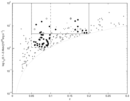
Figure 1: The $L_{X}-z$ distribution of the BCS visible during our observing run. The solid lines show the boundary of the high-luminosity volume-limited sample ($0.05<z<0.2$ and $L_{X}>4.46\times 10^{44}{\rm ergs^{-1}}$), and the dashed lines show the boundary of the low-redshift volume-limited sample ($0.05<z<0.1$ and $L_{X}>1.1\times 10^{44}{\rm ergs^{-1}}$). Large circles show clusters that we observed, with filled circles being those that we are presenting data for and open circles being those for which we could not process the images (see §2.2). Small points are clusters within our redshift and flux limits that we were not able to observe, and crosses show other clusters in the parent sample.

X-ray selection guarantees that the clusters we are observing are genuine massive bound systems, and not chance alignments of galaxies. This would affect examinations of BCG properties with, for example, cluster richness or the distribution of other cluster members.

Another reason for using X-ray selected clusters is that data is available to allow us to ensure our BCG candidates are the central cluster galaxies we want to study. For a few clusters in our sample the BCG is not immediately obvious as the second-ranked cluster member appears to have a similar magnitude (Bautz-Morgan type II clusters). Knowledge of the position of the X-ray centroid therefore allows the most central cluster galaxy to be identified in these ambiguous cases.

.

Table 1: BCG/Cluster parameters. Redshifts and X-ray characteristics are taken from Ebeling et al. (1998, 2000).

Cluster	$\alpha_{XRAY}$	$\delta_{XRAY}$	$\alpha_{BCG}$	$\delta_{BCG}$	Offset (”)	Offset (kpc)	$L_{X}$ ($10^{44}$ erg/s)	z
A0971	10:19:55.2	40:59:45.6	10:19:52.1	40:59:18.8	54.2	92.3	1.44	0.093
A1126	10:53:48.7	16:50:31.2	10:53:50.3	16:51:03.0	39.5	62.6	1.15	0.086
A1190	11:11:28.6	40:49:48.0	11:11:43.6	40:49:14.7	228.2	338.1	1.47	0.079
A1246	11:23:54.5	21:29:16.8	11:23:58.8	21:28:46.7	71.3	224.2	7.62	0.190
A1589	12:41:18.0	18:33:03.6	12:41:17.5	18:34:28.2	84.9	114.8	2.39	0.072
A1602	12:43:28.3	27:17:09.6	12:43:24.7	27:16:50.0	57.7	188.4	4.96	0.200
A1668	13:03:44.9	19:16:37.2	13:03:46.6	19:16:17.5	31.7	38.2	1.61	0.063
A1672	13:04:20.4	33:36:03.6	13:04:27.2	33:35:14.0	114.3	356.0	4.90	0.188
A1677	13:05:53.1	30:53:09.6	13:05:50.8	30:54:17.7	75.8	231.2	6.24	0.183
A1728	13:23:30.2	11:17:45.6	13:23:31.7	11:18:08.1	31.5	52.9	1.29	0.091
A1767	13:36:07.7	59:12:39.6	13:36:08.2	59:12:24.2	17.5	23.1	2.47	0.070
A1775	13:41:50.4	26:22:55.2	13:41:49.2	26:22:24.1	36.0	49.0	2.91	0.072
A1795	13:48:52.3	26:35:52.8	13:48:52.5	26:35:35.3	17.8	21.1	11.27	0.062
A1800	13:49:27.6	28:06:21.6	13:49:23.6	28:06:27.0	60.5	84.9	3.05	0.075
A1809	13:53:06.0	5:09:28.8	13:53:06.4	5:08:59.7	29.6	43.7	1.61	0.079
A1831	13:59:12.5	27:58:40.8	13:59:15.1	27:58:34.0	39.3	45.8	1.90	0.061
A1885	14:13:43.7	43:39:39.6	14:13:43.7	43:39:45.8	6.2	10.2	2.40	0.089
A1914	14:26:02.1	37:50:06.0	14:25:56.7	37:48:59.3	105.7	305.2	18.39	0.171
A1927	14:31:03.6	25:37:40.8	14:31:06.8	25:38:01.8	52.5	87.8	2.14	0.091
A1991	14:54:31.0	18:39:00.0	14:54:31.5	18:38:32.6	28.6	32.0	1.38	0.059
A2029	15:10:54.9	5:43:12.0	15:10:56.1	5:44:41.8	91.5	131.2	15.29	0.077
A2033	15:11:23.5	6:19:08.4	15:11:26.5	6:20:57.1	117.8	179.1	2.57	0.082
A2034	15:10:10.8	33:30:21.6	15:10:11.7	33:29:10.8	72.1	146.4	6.85	0.113
A2055	15:18:41.3	6:12:39.6	15:18:45.8	6:13:56.7	102.2	189.8	4.82	0.102
A2061	15:21:17.0	30:38:24.0	15:21:20.6	30:40:15.5	123.5	179.5	3.95	0.078
A2065	15:22:26.9	27:42:39.6	15:22:24.0	27:42:51.9	45.3	61.7	4.94	0.072
A2108	15:40:09.1	17:52:40.8	15:39:46.4	17:50:09.4	372.5	628.2	1.97	0.092
A2110	15:39:48.5	30:42:57.6	15:39:50.8	30:43:03.9	35.2	63.0	3.93	0.098
A2124	15:45:00.0	36:03:57.6	15:44:59.0	36:06:34.8	158.0	195.9	1.35	0.065
A2148	16:03:02.2	25:24:14.4	16:03:19.8	25:27:13.4	320.0	524.7	1.39	0.089
A2175	16:20:30.7	29:53:31.2	16:20:31.1	29:53:28.2	7.0	12.4	2.93	0.097
A2244	17:02:40.1	34:03:46.8	17:02:42.6	34:03:34.4	38.9	69.0	9.34	0.097
A2249	17:09:48.5	34:28:26.4	17:09:48.7	34:27:32.8	53.7	80.3	3.95	0.080
A2254	17:17:45.9	19:40:22.8	17:17:46.0	19:40:49.0	26.3	78.2	7.73	0.178
A2255	17:12:43.7	64:03:43.2	17:12:28.8	64:03:38.5	222.5	335.4	4.94	0.081
A2256	17:04:02.4	78:37:55.2	17:04:27.3	78:38:25.1	374.9	416.6	7.11	0.058
A2312	18:53:48.2	68:23:06.0	18:54:06.2	68:22:58.6	270.0	460.6	1.89	0.093
A2315	19:00:46.5	69:58:30.0	19:00:16.6	69:56:59.6	457.9	787.3	1.64	0.094
A2457	22:35:40.3	1:31:33.6	22:35:40.8	1:29:05.9	147.9	167.0	1.44	0.059
A2495	22:50:17.1	10:55:01.2	22:50:19.7	10:54:12.5	62.9	90.5	2.98	0.077
A2626	23:36:34.1	21:07:40.8	23:36:30.5	21:08:47.1	85.1	92.2	1.96	0.057
A2637	23:38:57.8	21:25:55.2	23:38:53.3	21:27:52.6	135.7	180.9	1.54	0.071
RXJ1326	13:26:18.0	0:13:33.6	13:26:17.6	0:13:17.9	16.7	25.6	1.69	0.082
RXJ1442	14:42:17.5	22:18:03.6	14:42:19.4	22:18:11.5	29.0	51.4	2.66	0.097
RXJ1750	17:50:16.1	35:04:58.8	17:50:16.7	35:04:57.9	9.6	27.8	5.49	0.171
Z4905	12:10:17.0	5:23:31.2	12:10:16.8	5:23:09.6	21.8	31.4	1.20	0.077
Z5029	12:17:41.3	3:39:32.4	12:17:41.1	3:39:21.7	11.1	15.6	5.28	0.075
Z6718	14:21:36.2	49:32:38.4	14:21:35.8	49:33:03.0	25.5	34.1	1.24	0.071
Z9077	23:50:34.5	29:31:51.6	23:50:37.5	29:29:07.6	169.7	295.7	2.11	0.095

¹R.A. of cluster X-ray emission peak

²Dec of cluster X-ray emission peak

³R.A. of BCG centre in $r^{\prime}$ band

⁴Dec of BCG centre in $r^{\prime}$ band

⁵Offset between X-ray peak and BCG centre in arcsec

⁶Offset between X-ray peak and BCG centre in kpc

2.2 Observations

Our data were obtained during a single seven-night run in May/June 2003, using the 2.5m Isaac Newton Telescope (INT) at the Roque de Los Muchachos Observatory, La Palma, Spain. The images were taken with the Wide Field Camera (WFC), which is a four-CCD mosaic camera with a field of view of $\sim 34^{\prime}\times 34^{\prime}$, and a scale of $0^{\prime\prime}.33$/pixel. Each processed cluster image is composed of two offset WFC pointings; the BCG is centered on chip 4 of the camera in one pointing, and chip 2 in the other (see figure 2). Chip 2 of pointing 1 does not form a contiguous part of the combined image and since each chip has a different gain, determining the correct sky level for chip 2 and still allowing for any large-scale sky gradients is extremely difficult. Hence, it is not included in the final mosaic. Rejection of this single chip gives a total field size of $\sim 41^{\prime}\times 41^{\prime}$. Exposures were taken in Harris $B$ (which closely mimics Johnson $B$ — Salzer et al. 2000) and Sloan $r^{\prime}$ filters, typically with all $B$ mosaics being a combination of $2\times 600s$ exposures, and the $r^{\prime}$ mosaics being $2\times 300s$. Higher $z$ clusters were observed for longer (see table 2). Photometry was calibrated using Landolt standard fields (Landolt 1992). The Cousins $R$ magnitudes used by Landolt were converted to Sloan $r^{\prime}$ using the relations determined by Smith et al. (2002):

$$r^{\prime}=\left\{\begin{array}[]{ll}V-0.44(B-V)+0.12&(V-R\leq 1.00)\\ V-0.81(V-R)+0.13&(V-R>1.00)\end{array}\right.$$ (1)

Conditions were photometric during the entire run, and seeing averaged at $1^{\prime\prime}.2$. Sky surface brightnesses, large-scale surface brightness uncertainties and exposure times are given in table 2. The uncertainties give, in effect, the level to which our measured surface brightnesses are reliable. A more complete explanation of the importance and calculation of these large-scale uncertainties is given in $\S 3.4$.

Table 2: Observational parameters. The left and right columns give the quantities for the $B$ band and $r^{\prime}$ band observations, respectively. See $\S 3.4$ for more about large-scale errors (LSE).

Cluster	Sky level		LSE		Exposure time
	$B$	$r^{\prime}$	$B$	$r^{\prime}$	$B$	$r^{\prime}$
A0971	21.88	20.78	28.36	27.02	600	300
A1126	22.13	20.88	28.88	27.87	600	300
A1190	22.12	21.06	28.78	28.20	600	300
A1246	22.23	20.95	28.90	28.21	600	600
A1589	22.34	21.23	28.93	27.98	600	300
A1602	22.39	21.10	28.83	28.02	600	600
A1668	22.47	21.19	28.78	28.13	600	300
A1672	22.62	21.18	29.34	28.82	600	600
A1677	22.57	21.36	29.20	28.61	600	600
A1728	22.35	21.02	29.17	28.24	600	300
A1767	22.47	21.19	28.94	27.80	600	300
A1775	22.41	21.23	29.21	28.29	600	300
A1795	22.40	21.16	28.85	28.04	600	300
A1800	22.60	21.44	29.22	28.33	600	300
A1809	22.27	21.16	28.58	27.99	600	300
A1831	22.38	21.37	28.88	27.81	600	300
A1885	22.60	21.41	28.98	28.08	600	300
A1914	22.45	21.26	28.83	28.44	900	450
A1927	21.57	21.36	28.29	28.36	300	300
A1991	22.41	21.32	28.97	28.15	600	300
A2029	22.29	21.02	28.96	28.51	600	300
A2033	22.22	21.04	28.91	28.20	600	300
A2034	22.48	21.30	28.97	27.97	900	450
A2055	21.64	20.86	28.42	27.61	900	450
A2061	22.21	21.20	28.63	27.82	600	300
A2065	22.45	21.12	28.73	27.65	600	300
A2108	22.38	21.25	28.74	28.09	600	300
A2110	22.46	21.32	29.04	28.40	600	300
A2124	22.41	21.20	29.05	28.07	600	300
A2148	22.51	21.32	28.60	27.60	600	300
A2175	22.46	21.39	28.64	27.80	600	300
A2244	22.46	21.34	28.49	27.42	600	300
A2249	22.53	21.34	28.62	27.74	600	300
A2254	22.35	21.23	28.58	28.30	600	600
A2255	22.33	21.10	28.67	28.04	600	300
A2256	22.20	20.76	28.38	27.55	600	300
A2312	22.29	21.05	28.15	27.60	600	300
A2315	22.32	21.04	28.32	27.64	600	300
A2457	21.94	20.66	28.07	27.25	600	300
A2495	21.88	20.74	28.23	27.60	600	300
A2626	22.13	20.85	28.28	27.65	600	300
A2637	22.00	20.87	28.41	27.70	600	300
RXJ1326	21.83	20.86	28.92	28.34	900	450
RXJ1442	22.30	21.09	29.08	28.23	600	300
RXJ1750	22.54	21.50	28.63	27.88	900	450
Z4905	22.27	20.96	28.92	28.97	600	300
Z5029	22.33	20.86	29.01	27.98	600	300
Z6718	22.46	21.26	28.37	27.80	600	300
Z9077	22.08	20.87	28.25	27.51	600	300

¹Sky surface brightness and LSE in mags/arcsec^2
2Exposure time for a single pointing, in seconds

Figure 1 shows that we observed all clusters in our lower $z$ bin but that we are only $\sim 60\%$ complete in the higher $z$ range. However, there is no obvious bias in the higher $z$ selection. Out of the 60 clusters we did observe, we were not able to extract reliable surface brightness profiles for the BCGs for 11 of them (A1773, A2142, A2187, A2204, A2218, A2259, A2396, A2409, RXJ1720, RXJ1844 and Z8276) due to contamination by foreground sources.

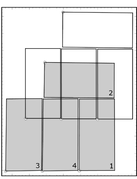
Figure 2: Mosaic combination of WFC pointings. Each of the final mosaics was made up of two pointings, one centred on chip 4 of the WFC, the other centred on chip 2. The shaded (lower) pointing is pointing 2, the unshaded is pointing 1. Chip 2 of pointing 1 is not included in the final mosaic as it does not overlap with any other part of the image. The numbers show the position of each of the WFC chips, which have active regions of $2048\times 4100$ pixels. The field of view of the mosaic is $\sim 41^{\prime}\times 41^{\prime}$.

3 Reductions

There are two critical factors which limit the measurement of low surface brightness features at large radii: the accuracy of flat-fielding and that of sky subtraction. The importance of these is pointed out in several other studies looking for intracluster light; for instance, Feldmeier et al. (2002) spent half their observing time taking blank sky images in order to construct sky flats, whilst Krick, Bernstein & Pimbblet (2006) used a third of their observing time for the same process. Due to the large number of observations we have, and the offsetting between pointings of the same cluster, we were able to construct our sky flats from our object images. This procedure is described in detail below, along with our sky subtraction algorithm.

3.1 Standard Reductions

Data were reduced using a combination of IRAF and Starlink routines. Full two-dimensional debiassing was necessary, after which bad pixels were found (by median combining the frames for each chip on a night-by-night basis) and fixed. The WFC is known to have non-linearities in all its chips, and these were corrected for using the following equations (Mike Irwin, private communication):

.

$$\begin{array}[]{ll}CCD_{1,true}&=x-2.5\times 10^{-6}x^{2}+1.2\times 10^{-11}x^{3}\\ CCD_{2,true}&=x-0.5\times 10^{-7}x^{2}-4.0\times 10^{-12}x^{3}\\ CCD_{3,true}&=x-6.0\times 10^{-7}x^{2}\\ CCD_{4,true}&=x-1.5\times 10^{-7}x^{2}-2.0\times 10^{-12}x^{3}\end{array}$$ (2)

.

Note that $CCD_{i,true}$ are the corrected counts (ADU) and that $x$ are the raw, (bias-subtracted) values.

Twilight flats were used as an initial correction for the images. However, sky flats were needed for the full correction and these were constructed from our object images. As can be seen in figure 2, each final mosaic is made up of two pointings, one with the BCG centred on chip 4 (this is defined as pointing 1) of the WFC, the other centred on chip 2 (pointing 2). Therefore, all chip 4 frames from pointing 1 were automatically rejected from the construction process, as were all chip 2 frames from pointing 2. Every remaining frame was then inspected and rejected if it contained large bright sources or other defects. In order to keep signal-to-noise the same across the mosaic, the same number of frames was used to make the master sky flat for each chip.

The master sky flats were constructed using a procedure based on that of Morrison et al. (1997) and Feldmeier et al. (2002). First, SExtractor (Bertin & Arnouts 1996) was used to pick out sources down to a threshold of $1\sigma$ above the background and create an object mask. The IRAF task mimstat was next used with this mask to calculate the modal value for each accepted frame. The frames were then normalised by their modes and median combined with IRAF’s imcombine, using a sigma-clipping ($\pm 2\sigma$) algorithm. Each of the individual sky frames was finally corrected with this master flat, and their modes were recalculated. The cycle was then restarted, with the original accepted frames now being normalised by their recalculated modes. This cycle of corrections successively reduces the distribution of sky values in the image and allows a more accurate determination of the modal value of the image. 4 such cycles were sufficient as by that point the percentage difference between modal values was of the order of $10^{-8}$. All object frames were divided by these final flats.

Before combining the frames to make the final two-pointing mosaic, a correction was needed to account for the nonlinear ’pincushion’ distortion inherent to the WFC optical system. Calibrated co-ordinate information specific to the WFC is available in the Starlink ASTIMP task in the CCDPACK suite of software. CCDPACK tasks were also used for the registering and mosaicing of the images, and for the level-matching between chips which was necessary due both to the different gain of each WFC chip, and for the background differences between the two pointings.

3.2 Astrometry

For each mosaic, an initial World Coordinate System was fitted using $\sim 10$ stars identified from Digitized Sky Survey (DSS) plates through the ALADIN Java applet (Bonnarel et al. 2000). Tasks from the WCSTools package (Mink 2002) were then used to locate a much larger number of stars (typically $\sim$ 100) from the USNO-A2.0 catalogue (Monet et al. 1998). These positions were refined interactively and the final WCS was set by IRAF tasks using a fifth-order Legendre polynomial. Fitting the WCS allowed us to check that the BCGs being analysed in our images were the ones nearest the cluster X-ray peaks, an important point which has already been mentioned above. The r.m.s. errors in the fitting, combined with the positional errors in the USNO-A2.0 catalogue (Deutsch 1998), give total uncertainities of the order of $<0^{\prime\prime}.8$ for image positions.

3.3 Masking

Accurately modelling the BCG profile at very low surface brightnesses requires that contaminating sources are adequately masked. SExtractor was used to pick out objects for masking and there are two main parameters that need to be set for object detection: the detection threshold and the minimum number of contiguous pixels that constitute an object. We chose to mask down to a threshold of $0.8\sigma$ above the background. However, at this level there is a danger of overmasking as it is easy to mistake noise spikes for real objects if the minimum object area is set too low. To determine an appropriate minimum area, for each image SExtractor was first run with a $0.8\sigma$ threshold for a range of object areas from 5 to 20 pixels and the number of objects detected at each area setting was found. SExtractor was then run again in the same way on the negative version of the image. All objects detected in the negative image should be noise peaks and not real objects. If we assume that noise is distributed equally about the sky level, then the distribution of detections in the positive image minus the distribution of detections in the negative image will give the distribution of real objects as a function of minimum area (figure 3). As a compromise between masking too many noise spikes and not masking enough objects, the minimum detection area was finally set at the area at which the number of real objects was equal to the number of noise spikes being picked up. These detection limits correspond to a magnitude threshold (for point-like objects) of $m_{B}\sim 26.7$ and $m_{r^{\prime}}\sim 25.9$. An examination of the number counts of objects in the masking catalogues shows that we are complete down to $m_{B}\sim 25.8$ and $m_{r^{\prime}}\sim 25.0$.

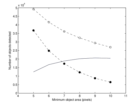
Figure 3: Numbers of objects detected as a function of minimum area for the B-band image of A2029. The open circles show the distribution of detections in the positive image and the filled circles show the distribution of detections in the negative image. The solid line is the difference between these and should be the distribution of real objects. The SExtractor minimum area parameter was chosen as the point where noise and object detections are equal.

SExtractor was then run to produce both an object catalogue and a segmentation image. Shape information from the output catalogue was used to produce an object image, with the major and minor axes of each object being scaled by its magnitude. The object and segmentation image were then combined to produce the final mask. The same mask was used for both $B$ and $r^{\prime}$ versions of each image to ensure consistent colour measurements, with the mask being based on the $r^{\prime}$ image as it is deeper than the $B$ image. Similarly to Krick et al. (2006), for each cluster two additional masks were produced with the magnitude-scaled major and minor axes shrunk by 10% and grown by 10%, in order to investigate the effect mask size has on the extracted BCG profile. Table 3 gives the percentage of each image masked. Typically the masking procedure removes $\sim 25\%$ of the pixels from the images around each BCG, as listed in Table 2. The third column in the table gives the proportion of the area masked around the BCG out to the maximum radius of the software-generated BCG model. Figure 4 shows the ’best’ and ’worst’ cases from this column: The $r^{\prime}$ band image of the BCG in A2256 has $\sim 46\%$ of its area masked whereas only $\sim 14\%$ of the area around the BCG in the $r^{\prime}$ band image of Z4905 is masked.

Table 3: Extent of masking. Column 2 gives the percentage of the total area of the image that has been masked and the values in column 3 give the percentage of the profile area that has been masked in the $B$ and $r^{\prime}$ bands, respectively. These values are different as profiles often extend further in $r^{\prime}$.

Cluster	% of total area	% of profile area
		$B$	$r^{\prime}$
A0971	15.2	22.4	21.4
A1126	14.9	26.4	28.6
A1190	19.4	21.2	21.2
A1246	13.6	26.0	33.3
A1589	17.4	31.8	30.1
A1602	17.4	34.6	25.7
A1668	14.7	21.7	21.7
A1672	16.7	20.8	20.8
A1677	17.7	28.3	33.8
A1728	14.8	15.4	14.1
A1767	18.8	24.6	25.0
A1775	16.3	17.8	17.8
A1795	19.4	19.5	20.2
A1800	19.4	21.9	21.2
A1809	15.1	24.2	26.2
A1831	16.4	30.7	30.6
A1885	13.2	15.6	16.1
A1914	13.8	32.2	32.2
A1927	21.4	21.3	21.2
A1991	16.4	20.2	21.2
A2029	19.7	30.6	25.2
A2033	20.2	27.0	27.0
A2034	19.9	29.1	29.1
A2055	16.3	30.5	30.0
A2061	18.2	27.4	22.9
A2065	16.4	28.6	31.7
A2108	18.8	21.1	21.8
A2110	16.0	19.7	19.7
A2124	14.8	25.5	25.4
A2148	17.4	19.0	18.1
A2175	20.8	27.0	26.7
A2244	24.3	33.3	33.2
A2249	20.9	32.4	30.7
A2254	32.0	45.7	43.7
A2255	22.6	37.2	29.4
A2256	21.1	45.9	33.5
A2312	25.8	27.2	28.6
A2315	21.3	21.8	23.2
A2457	23.4	30.3	30.3
A2495	15.4	18.9	20.0
A2626	19.2	22.9	24.4
A2637	16.2	21.0	19.5
RXJ1326	17.6	17.1	18.9
RXJ1442	13.2	21.6	22.6
RXJ1750	23.0	29.6	28.9
Z4905	12.8	13.6	15.9
Z5029	17.5	22.6	22.1
Z6718	17.4	18.6	18.6
Z9077	23.4	23.7	24.7

Figure 4: Masked images of the BCGs in A2256 (left) and Z4905 (right). Both are $r$ band images with the levels scaled logarithmically. These images represent the extremes of the masking procedure, with Z4905 having 13.6% of the profile area removed from the isophote-fitting process and A2256 having 45.9% removed.

3.4 Sky subtraction

Accurate sky subtraction is crucial when attempting to measure surface brightnesses down to the level we require. We used an iterative procedure to remove the sky, which acted to improve our sky model with each cycle:

1. A large region around and including the BCG was masked out to a radius of 0.5Mpc from the BCG centre. This value was chosen as we did not expect to find any ICL beyond this at the depth of our images (Gonzalez et al. 2005, Zibetti et al. 2005). This was combined with the mask produced through the technique described above and used to reject points from a surface-fitting task (Starlink’s SURFIT). The extent of the background sampled by our images ($\sim 41^{\prime}\times 41^{\prime}$) deems it necessary to allow for large-scale gradients in the sky level and so a planar surface was fit to the background.

2. The IRAF ellipse task (Busko 1996, Jedrzejweski 1987) was used to model and remove any large bright stars and galaxies (including the BCG) from the image. The ellipse ellipticity parameter is normally required to be between 0.05 and 1 but the parameter set was edited to allow it to be as low as 0.001 (the ellipse-fitting algorithm diverges at $e=0$) and fixed at this value to accurately model the circular stellar isophotes.

3. The surface previously subtracted was then added back to the source-removed image and a new planar sky was calculated, as a better estimate of the actual background is made possible by the removal of bright sources.

This cycle was run 3 times for each image. For the first of these cycles, an additional step was included between (2) and (3) in which a new mask was produced. This mask covered the diffraction spikes and saturated regions of the bright stars removed in step (2) and allowed better stellar models in subsequent cycles.

In order to check our large-scale flat-fielding and sky subtraction errors, we followed the approach outlined in Feldmeier et al. (2002). We binned up our final reduced, sky-subtracted images into $50\times 50$ pixel sections and calculated the median value of each bin. Each bin had to have at least half its pixels unmasked for its value to be accepted, and histograms of these medians were then created. Two examples are shown in figure 5. The widths of these histograms around zero are in effect a measure of the above errors, as the dispersion is due to flat-fielding errors and excess contaminating light which we have failed to mask. The mean sky values for the images shown, which are of the clusters A1672 and A2029, were 437.2 ADU and 1145.5 ADU respectively, which we estimate give us uncertainties of 0.16% ($\sigma=0.69$ ADU) and 0.09% ($\sigma=1.04$ ADU) for residual flat-fielding and sky-subtraction errors. The uncertainties for the full sample are provided in table 2.

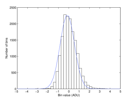
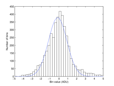
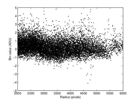
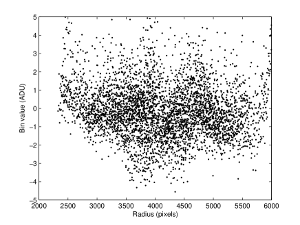
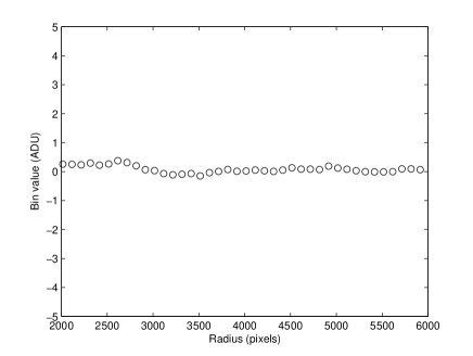
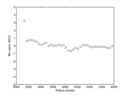
Figure 5: Histograms of background values for the images of A1672 ($B$) (left) and A2029 ($r^{\prime}$) (right), calculated after flat-fielding and sky subtraction. The bins have widths of 0.25ADU and the overlaid Gaussian fits have an r.m.s. of 0.69ADU and 1.04ADU, respectively (corresponding to surface brightnesses of $\mu_{B}=29.34$ and $\mu_{r}=28.51$). These histograms allow us to quantify our large-scale errors, which need to be as low as possible to reliably detect faint ICL. The middle plots give the median value of the bins as a function of distance from the centre of each image, whilst the lower plots show the running median of 100pixel radius intervals. They show that there appears to be no significant correlation of residual value with position.

3.5 Comparison with Star Subtraction

Instead of masking all objects in an image, the usual approach to taking care of contaminating sources in an image is to first subtract off the stars, and then mask out the remaining unwanted features. We opted for full masking as it was a technically less complex approach and we judged it to be less likely to introduce errors in sky subtraction. An incorrect PSF model will have a detrimental effect on the sky model as stars may be under- or oversubtracted, but this is avoided by simply masking out the stars and rejecting them from the fitting. The main driving factor, however, was the speed of the masking process compared to one involving star subtraction, which is an important consideration for our project due to both the large size and number of our images.

To ensure that we were not sacrificing accuracy for speed, for a few test images we implemented a star subtraction algorithm. The basis for this was to produce a good PSF model that would account not only for the central regions of stars but also for the extended outer regions, as faint residual light is our main problem. As in Feldmeier et al. (2002) and Gonzalez, Zabludoff & Zaritsky (2005), we constructed a large-radius PSF using the cores of unsaturated stars and the wings of brighter, saturated stars as these contain high signal-to-noise. This model was used to create a star-subtracted image which was used as the initial input for the iterative masking process described in §3.3. Comparisons of the final 1D profiles calculated by ellipse using the star-subtraction and masking-only methods are shown in figure 6, for two of our tests, A2249 and A2029. It is clear that the profiles agree extremely well, even down to the lowest surface brightnesses we can reach.

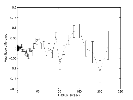
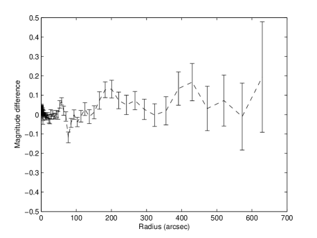
Figure 6: Plots of the difference between the surface brightness profiles calculated using the star-subtraction and masking-only methods, for the BCGs in A2029 (top) and A2249 (bottom). See main text for an explanation of the differences in these approaches. As the profiles show, the simpler and less time-consuming masking-only approach produces profiles which agree very well with the star-subtraction method, even at the faint ends of the profiles, with no appreciable systematic difference in magnitude with radius. The error bars are based on the uncertainty in isophotal intensity.

4 Results

For each of the observed BCGs, figure LABEL:galpics shows a $300^{\prime\prime}\times 300^{\prime\prime}$ image in $r^{\prime}$.

Radial profiles were calculated from the masked image in each pass-band for all target galaxies, using the mask produced from the $r^{\prime}$ band image. We used the masking-only method of removing foreground objects. As discussed in $\S 3.4$, this method is as reliable as subtracting stars using a PSF fit, and is also faster and more robust. As mentioned in $\S 3.3$, we used the IRAF ellipse task to make the measurements. The radii of the isophotes were chosen to follow a geometric progression and the centroids were kept fixed. The resulting surface brightness profiles are plotted in figure LABEL:galpics, along with colour, ellipticity, and position angle profiles. To ensure consistency in colour measurements, colour profiles were calculated using the geometry information for the $r^{\prime}$ band isophotes for both the $r^{\prime}$ and $B$ images.

Error limits for the surface brightness and colour profiles come from combining large-scale errors ($\S 3.4$), an estimate of star/galaxy light missed from the masking procedure (using the ’grown’ and ’shrunk’ masks), and the scatter of intensities along the isophotes. In virtually all cases, the last two sources of uncertainty are negligible, even at the faint ends of the profiles. Instead, the uncertainty is dominated by the effects of flat-field inhomogeneities and imperfect sky subtraction. However, the errors shown in the profiles and table 2 will be an overestimate of the uncertainty as we are considering variations and missed light across the entire image not just the area covered by the host cluster of the BCG.

5 Discussion

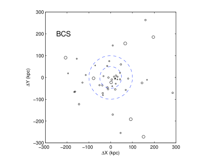
Figure 7: Offset between the BCG centre and the X-ray emission peak of its host cluster (from the BCS). The inner dashed circle has a radius of 50kpc and the outer is 100kpc. The size of each marker is the error in position associated with the calculated offset. The mean offset between the peaks and centres is 129.0kpc, with an r.m.s. of 122.0kpc.

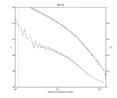
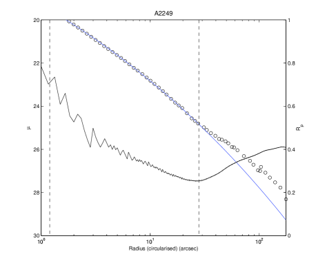
Figure 8: Surface brightness and Petrosian $R_{p}(=1/\eta)$ profiles for the BCGs in A2124 and A2249. Plotting $R_{p}$ to examine the behaviour of the BCG light profile means that determining the limits of the Sérsic fit becomes much less subjective, which is particularly important when the BCG appears to have a halo, as is the case for A2249. Note that the innermost dashed lines denote the seeing radii and the outer dashed line in the plot of A2249 is the radius outside which data is excluded from the Sérsic fit.

We have presented basic data in the form of surface-brightess, ellipticity and position angle profiles for a large sample of BCGs. In a further series of papers we intend to perform a variety of analyses on our data set, including an examination of the morphological properties of the BCGs, the investigation of substructure, and surface brightness profile fitting.

For our 49 clusters we find that in 22 cases the centre of the BCG is less than 100kpc from the centre of the X-ray isophotes taken from the BCS survey (Ebeling et al. 1998, 2000). Cypriano et al. (2004) found a similar alignment for 17 of the 22 clusters they examined for a weak lensing study. We note that the cluster X-ray positions obtained from the NORAS catalogue (Böhringer et al. 2000) have an RMS scatter of 95kpc compared to the BCS positions, so this scatter is largely related to the difficulty of defining the isophotal centre. In two cases there is a discrepancy in excess of 0.5Mpc between the purported X-ray centre and the location of the BCG. Closer examination of these cases reveals that both these objects have significant levels of substructure with obvious large sub-clumps. Such a close agreement between the centre of the mass distribution and the location of the BCG indicates a cuspy mass profile with a small or negligible core, in agreement with modern simulations of large clusters (Navarro, Frenk & White 1996; Moore et al. 1998; Power et al. 2003) which readily produce such profiles. It also supports the contention of Allen (1998) that the discrepancy between X-ray and gravitational lensing mass estimates for clusters of galaxies was due to an overestimation of the core size in so-called non-cooling flow clusters that was not present in the underlying mass distribution. Such a conclusion had already been reached by Smail et al. (1995) using strong lensing measurements.

It is thought that BCGs form early in the history of their host clusters (Merritt 1985, Tremaine 1990) and that in general they will have grown little since then. Work by Conselice, Bershady and Jangren (2000) suggests that quantification of observed asymmetries coupled with colour information may allow us to determine whether a galaxy is involved in an interaction and therefore allow us to see how often events that contribute to the growth of the BCG actually occur at low redshifts.

Substructure within the cD envelope/ICL will also enable us to study the history of interactions. Large tidal debris arcs have been found in the Coma cluster (Trentham & Mobasher 1998; Gregg & West 1998) and the Centaurus cluster (Calcáneo-Roldán et al. 2000). Feldmeier et al. (2002) also report a tidal debris plume in MKW7 and further features in A1914 (Feldmeier et al. 2004). It has been proposed that these features arise from tidal interactions between cluster galaxies and the cluster potential (Moore et al. 1996) and such arcs have been seen in simulations following the evolution of intracluster stars (Willman et al. 2004).

It has long been known that BCGs have shallower surface brightness profiles than the de Vaucouleurs $r^{1/4}$ profile (de Vaucouleurs 1948), and it is this excess light over the $r^{1/4}$ profile which is usually termed the cD envelope. Beginning particularly with the work of Caon, Capaccioli & D’Onofrio (1993), many authors (see Graham & Driver, 2005, for an extensive list) are now favouring the $r^{1/n}$, or Sérsic (Sérsic 1968), profile as the universality of the $r^{1/4}$ is questionable. In addition, the exponent $n$ (often known as the shape parameter), rather than being simply an extra parameter with no physical basis, has been found to correlate with various other observable properties in a way that is not explained by parameter coupling, thus offering a much deeper insight into bulge-type systems than the $r^{1/4}$ law. The value of $n$ correlates with effective radius $r_{e}$ and the total luminosity of the system, such that more luminous galaxies have a larger value of $n$ (e.g. Caon, Capaccioli & D’Onofrio 1993); Graham, Trujillo & Caon (2001) show that $log(n)$ correlates with the the galaxy’s central velocity dispersion; and $n$, effective radius and central surface brightness are tightly distributed about a plane (the photometric plane) for ellipticals (Khosroshahi et al. 2000; Graham 2002; La Barbera et al. 2004; La Barbera et al. 2005; Ravikumar et al. 2006).

However, Sérsic fitting suffers from the following problem: given the presence of an envelope, the range of radii over which the model should be used to fit the surface brightness profile is difficult to determine. Although this problem also occurs with the $r^{1/4}$ law (Schombert 1986), it is made worse in the Sérsic case because of the extra degree of freedom. An interesting solution to this that we have found makes use of the Petrosian index, $\eta$ (Petrosian 1976). This is the ratio of the average intensity within some radius $(R)$ to the intensity at that radius:

.

$$\eta(R)=\frac{2\int_{0}^{R}I(R^{\prime})R^{\prime}dR^{\prime}}{R^{2}I(R)}$$ (3)

.

Figure 8 shows surface brightness profiles of the BCGs in A2124 and A2249, and their corresponding plots of $R_{p}$ ($=1/\eta$) as a function of radius. The monotonic decrease in the $R_{p}$ profile of A2124 implies that there is very little excess light found here, i.e. this galaxy does not appear to have an extended halo, and this can be seen in its surface brightness profile which is well fit at all radii by a Sérsic law. On the contrary, the other BCG shows an increase in $R_{p}$ at a radius of $\sim 30^{\prime\prime}$. The point at which $R_{p}$ increases can be translated as the point where we begin to see an envelope, and where the Sérsic fit to the surface brightness profile becomes unreliable. Note that the innermost dashed lines denote the seeing radii and the outer dashed line in the plot of A2249 is the radius outside which data is excluded from the Sérsic fit. However, we note that although we do see a correspondence in these two examples, a rigorous analysis is required to put this method onto a reliable footing, and we intend to carry this out in future work.

35 of the 49 BCGs show a very clear increase in ellipticity with radius, and this may mark the change from the stellar population of the BCG to that of the intracluster medium. Basilakos, Plionis & Maddox (2000) found that the distribution of ellipticities of clusters in the APM survey has a peak at $\epsilon=0.46$. This agrees well with the values for the outermost isophotes of many of our BCGs, suggesting that perhaps the outer regions are tracing the cluster potential.

As we have already mentioned, one of the major advantages of our data set is that we have imaging in both $B$ and $r^{\prime}$ bands, allowing colour gradients to be measured. Schombert (1988) considered two-component fits in order to derive properties for the cD envelope, and this was taken a step further by Gonzalez et al. (2005), who used full two-dimensional two-component fits. It will be extremely interesting to combine these approaches with colour analysis to understand the properties of the BCG and its envelope.

6 Acknowledgements

We thank the referee, Stefano Zibetti, for the excellent suggestions and useful commments that have significantly improved this manuscript. We would also like to thank Mark Taylor for his help with the Starlink packages used in this work.

PP acknowledges the support of a PPARC studentship. FRP is a PPARC Advanced Fellow. The Isaac Newton Telescope is operated on the island of La Palma by the Isaac Newton Group in the Spanish Observatorio del Roque de los Muchachos of the Instituto de Astrofisica de Canarias.

References

- Allen (1998) Allen S., 1998, MNRAS, 296, 392
- Aragón-Salamanca, Baugh, & Kauffmann (1998) Aragón-Salamanca A., Baugh C.M., & Kauffmann G., 1998, MNRAS, 297, 427
- Arnaboldi (2004) Arnaboldi M., 2004, Recycling Intergalactic and Interstellar Matter, IAU Symposium Series, Vol 217, ed. Pierre-Alain Duc, Jonathan Braine & Elias Brinks
- Basilakos, Plionis & Maddox (2000) Basilakos S., Plionis M., & Maddox S.J., 2000, MNRAS, 316, 779
- Beers & Geller (1983) Beers T.C., & Geller M.J., 1983, ApJ, 274, 491
- Bertin & Arnouts (1996) Bertin E., & Arnouts S., 1996, A&AS, 117, 393
- Bingelli (1982) Bingelli B., 1982, A&A, 107, 338
- Böhringer H. et al. (2000) Böhringer H., et al., 2000, ApJS, 129, 435
- Bonnarel et al. (2000) Bonnarel F., et al., 2000, A&AS, 143, 33
- Burke, Collins & Mann (2000) Burke D.J., Collins C.A., & Mann R.G., 2000, ApJL, 532, L105
- Busko (1996) Busko I.C., 1996, ASPC, 101, 139
- Calcáneo-Roldán et al. (2000) Calcáneo-Roldán C., Moore B., Bland-Hawthorn J., Malin D., Sadler E.M., 2000, MNRAS, 314, 324
- Caon, Capaccioli, & D’Onofrio (1993) Caon N., Capaccioli M., & D’Onofrio M., 1993, 265, 1013
- Collins & Mann (1998) Collins C.A., & Mann R.G., 1998, MNRAS, 297, 128
- Conselice, Bershady, Jangren (2000) Conselice C.J., Bershady M.A., & Jangren A., 2000, ApJ, 529, 886
- Crawford et al. (1999) Crawford C.S., Allen S.W., Ebeling H., Edge A.C., & Fabian A.C., 1999, MNRAS, 306, 857
- Cypriano et al. (2004) Cypriano E.S., Sodré L., Jr., Kneib J.-P., Campusano L.E., 2004, ApJ, 613, 95
- de Vaucouleurs (1948) de Vaucouleurs G., 1948, Ann. d’Ap., 11, 247
- Deutsch (1998) Deutsch E.W., 1998, AJ, 118, 1882
- Dubinski (1998) Dubinski J., 1998, ApJ, 502, 141
- Ebeling et al. (1998) Ebeling H., et al., MNRAS, 301, 881
- Ebeling et al. (2000) Ebeling H., et al., MNRAS, 318, 333
- Edge & Stewart (1991) Edge A.C., & Stewart G.C., 1991, MNRAS, 252, 428
- Feldmeier et al. (2002) Feldmeier J.J., Mihos J.C., Morrison H.L., Rodney S.A., Harding P., 2002, ApJ, 575, 779
- Feldmeier et al. (2004a) Feldmeier J.J., Mihos J.C., Morrison H.L., Harding P., Kaib N., Dubinski J., 2004a, ApJ, 609, 617
- Feldmeier et al. (2004b) Feldmeier J.J., Mihos J.C., Morrison H.L., Harding P., Kaib N., 2004b, Carnegie Observatories Astrophysics Series, Vol. 3: Clusters of Galaxies: Probes of Cosmological Structure and Galaxy Evolution, ed. J.S. Mulchaey, A. Dressler, A. Oemler
- Gonzalez, Zabludoff, & Zaritsky (2005) Gonzalez A.H., Zabludoff A.I., & Zaritsky D., 2005, ApJ, 618, 195
- Graham (2002) Graham A.W., 2002, MNRAS, 334, 859
- Graham & Driver (2005) Graham A.W., & Driver S.P., 2005, PASA, 22, 118
- Gregg & West (1998) Gregg M.D., & West M.J., 1998, Nature, 396, 549
- Jedrzejewski (1987) Jedrzejewski R.I., 1987, MNRAS, 226, 747
- Jones & Forman (1984) Jones C., & Forman W., 1984, ApJ, 276, 38
- Khosroshahi et al. (2000) Khosroshahi H.G., Wadadekar Y., Kembhavi A., & Mobasher B., 2000, 531, L103
- Krick, Bernstein & Pimbblet (2006) Krick J.E., Bernstein R.A., & Pimbblet K.A., 2006, AJ, 131, 168
- La Barbera et al. (2004) La Barbera F., et al., 2004, A&A, 425, 797
- La Barbera et al. (2005) La Barbera F., et al., 2005, MNRAS, 358, 111
- Landolt (1992) Landolt A.U., 1992, AJ, 104, 340
- Malamuth & Richstone (1984) Malamuth E.M., & Richstone D.O., 1984, ApJ, 276, 413
- Merritt (1985) Merritt D., 1985, ApJ, 289, 18
- Miller (1983) Miller G.E., 1983, ApJ, 268, 495
- Mink (2002) Mink D., 2002, ASPC, 281, 169
- Monet et al. (1998) Monet D., et al., 1998, The USNO-A2.0 Catalogue (U.S. Naval Observatory, Washington D.C.)
- Moore et al. (1996) Moore B., Katz N., Lake G., Dressler A., Oemler A., 1996, Nature, 379, 613
- Moore et al. (1998) Moore B., Governato F., Quinn T., Stadel J., Lake G., 1998, ApJ, 499, L5
- Navarro, Frenk & White (1996) Navarro J.F., Frenk C.S., & White S.D.M., 1996, ApJ, 462, 563
- Petrosian (1976) Petrosian V., 1976, ApJ, 209, L1
- Porter, Schneider, & Hoessel (1991) Porter A.C., Schneider D.P., Hoessel J.G., 1991, AJ, 101, 1561
- Postman & Lauer (1994) Postman M., & Lauer T.R., 1994, ApJ, 425, 418
- Power et al. (2003) Power C., et al., 2003, MNRAS, 338, 14
- Ravikumar et al. (2006) Ravikumar C.D., et al., 2006, A&A, 446, 827
- Romer et al. (2000) Romer A.K., et al., 2000, ApJS, 126, 209
- Salzer et al. (2000) Salzer J., et al., 2000, AJ, 120, 80
- Schombert (1986) Schombert J.M., 1986, ApJ, 60, 603
- Schombert (1988) Schombert J.M., 1988, ApJ, 328, 475
- Sérsic (1968) Sérsic J.-L., 1968, Atlas de Galaxias Australes, Observatorio Astronomico, Cordoba
- Smail et al. (1995) Smail I., et al. 1995, MNRAS, 277, 1
- Smith et al. (2002) Smith J.A., et al., 2002, AJ, 123, 2121
- Sommer-Larsen, Romeo, & Portinari (2005) Sommer-Larsen J., Romeo A.D., & Portinari L., 2005, MNRAS, 357, 478
- Tremaine (1990) Tremaine S., 1990, Dynamics and Interactions of Galaxies, ed. R. Wielen, 394
- Trentham & Mobasher (1998) Trentham N., & Mobasher B., 1998, MNRAS, 293, 53
- Willman et al. (2004) Willman B., Governato F., Wadsley J., Quinn T., 2004, MNRAS, 355, 159
- Zabludoff et al. (1993) Zabludoff A.I., Geller M.J., Huchra J.P., Vogeley M.S., 1993, AJ, 106, 1273
- Zibetti et al. (2005) Zibetti S., White S.D.M., Schneider D.P., Brinkmann J., 2005, MNRAS, 358, 949