Evolution of linear perturbations through a bouncing world model:
Is the near Harrison-Zel’dovich spectrum possible via a bounce?

Abstract

We present a detailed numerical study of the evolutions of cosmological linear perturbations through a simple bouncing world model based on two scalar fields. We properly identify the relatively growing and decaying solutions in expanding and collapsing phases. Using a decomposition based on the large-scale limit exact solution of curvature (adiabatic) perturbations with two independent modes, we assign the relatively growing/decaying one in an expanding phase as the $C/d$-mode. In the collapsing phase, the roles are reversed, and the $C/d$-mode is relatively decaying/growing. The analytic solution shows that, as long as the large scale and the adiabatic conditions are met, the $C$- and $d$-modes preserve their nature throughout the bounce. Here, by using a concrete nonsingular bouncing world model based on two scalar fields, we numerically follow the evolutions of the correctly identified $C$- and $d$-modes which preserve their nature through the bounce, thus confirming our previous anticipation based on the analytic solution. Since we are currently in an expanding phase the observationally relevant one in the expanding phase is the relatively growing $C$-mode whose nature is preserved throughout the bounce. The spectrum of $C$-mode generated from quantum fluctuations in the collapsing phase has a quite blue spectrum compared with the near Harrison-Zel’dovich scale-invariant one. Thus, while the large-scale condition is satisfied and the adiabatic condition is met during the bounce, we conclude that it is not possible to obtain the near Harrison-Zel’dovich scale-invariant density spectrum through a bouncing world model as long as the seed fluctuations were generated from quantum fluctuations of the curvature perturbation in the collapsing phase. We also study the tensor-type perturbation. For the tensor-type perturbation, however, both $C$- and $d$-modes (of the tensor-type perturbations) in the collapsing phase survive as the relatively growing $C$-mode in the expanding phase. Due to its growing nature in the collapsing phase, the initial $d$-mode dominates the surviving $C$-mode spectrum after the bounce.

I Introduction

In order to explain the large-scale structures and motions of the galaxy distribution and the temperature anisotropies of cosmic microwave background we need near Harrison-Zel’dovich scale-invariant spectrum for the initial density fluctuations which was suggested in the early 70’s HZ-spectrum . Currently, inflation (early acceleration phase) scenario provides the only known mechanism which can successfully generate seed fluctuations for such cosmological structures. Inflation provides near Harrison-Zel’dovich spectrum rather naturally by amplifying the ever present quantum fluctuations in the matter and space-time in microscopic scales during an early acceleration phase.

Recently, several bouncing cosmological world models were suggested as alternatives to the inflation scenario. The pre-big bang scenario pbb is based on the low-energy tree-level string theory effective action. However, pre-big bang scenario fails to explain the current large-scale structure because the generated spectrum is quite bluer than near Harrison-Zel’dovich spectrum, see pbb-pert . More recently, ekpyrotic and cyclic scenarios Ek were suggested based on the collision of two branes in a five dimensional bulk. According to the authors of these scenarios, near Harrison-Zel’dovich spectrum follows from the $d$-mode of curvature perturbation in the zero-shear gauge ($\varphi_{\chi}$; terms will be explained shortly). Such a claim has been disputed by several authors Lyth ; BF ; hw1 ; hw2 ; HN-bounce . We pointed out that although the $d$-mode is the dominating mode in the collapsing phase it decays away as the background model switches to expanding phase, thus irrelevant observationally hw1 ; hw2 ; HN-bounce . Also the $d$-mode of $\varphi_{\chi}$ is known to exaggerate the perturbations due to overly distorted hypersurface (temporal gauge) condition compared with the curvature perturbation in the comoving gauge ($\varphi_{v}$), see Bardeen-1980 . In fact, the authors of cyclic scenario in Ek claimed that in effective four dimensional space-time their world model goes through a singularity. In such a case not only the background world model, but also the perturbations inevitably become singular, thus we have no tool to handle the situation Lyth . In order to handle the situation theoretically in hw1 ; hw2 ; HN-bounce we have considered several smooth and nonsingular bouncing world model assuming both the background world model and linear perturbations remain valid. The present work is a continuation of our previous studies using a specific bouncing world model and concrete numerical study of perturbations under such a bounce.

Here we summarize our previous reason, for not considering the $d$-mode as seed fluctuations, used in hw1 ; hw2 ; HN-bounce . A scalar-type cosmological perturbation of a single component medium is described by a second-order differential equation. As long as the large-scale condition is met we have an analytic solution with two independent modes which we term $C$- and $d$-modes, see Sec. III.1. We assign the relatively growing/decaying one in an expanding phase as the $C/d$-mode; in the collapsing phase, the roles are reversed, and the $C/d$-mode is relatively decaying/growing. In fact, for $\varphi_{v}$ the $C$-mode simply remains constant in time and the $d$-mode decays in an expanding phase, thus suggesting their names. Since such a large-scale condition is well met near the bounce we are considering, we anticipate the nature of the $C$- and $d$-modes to be preserved even after the bounce. Because the observationally relevant one in the expanding phase is the relatively growing $C$-mode, even in the collapsing phase, we have to consider the seed perturbation in the $C$-mode generated from quantum fluctuations. This shows quite blue spectra both for the pre-big bang and the ekpyrotic (or cyclic) scenarios. Although not successful as alternative to the inflation, these models have spurred interests in the evolution of perturbations through nonsingular bounces in the early universe bounce-pert-others ; FB ; AW . In this work we will show the same conclusion, now using a numerical study of perturbation through a specific nonsingular bouncing world model.

In order to have a realistic bounce in practice, we have to consider an additional field or fluid component which drives the nonsingular bounce in additional to the field or fluid which gives rise to the seed fluctuations for the large-scale structures HN-bounce ; bounce-pert-others . In such cases we have to consider perturbations of the additional field introduced to have bounce, in addition to the field for fluctuation seeds. Even in such cases, however, we expect our above conclusion based on the analytic solutions for the single component is relevant for the analysis; for our previous analytic argument, see Sec. V.C of HN-bounce . Recently, however, authors of AW have reported that by numerical analysis, for a specific collapse phase, the $d$-mode of $\varphi_{v}$ in the collapsing phase survives as the $C$-mode in the expanding phase, thus allowing a scale-invariant spectrum available for that specific collapse, see also Wands-1999 ; FB ; BF . The numerical results in AW show the growing mode ($d$-mode) in a collapsing phase survives as the growing mode ($C$-mode) in an expanding phase. In this work we will show that this is a result based on mixed initial conditions of our precise $C$- and $d$-modes; the latter initial conditions produce evolutions where $C$- and $d$-mode natures are preserved even after the bounce.

In this work, we would like to address and clarify whether switching of $d$-mode to the $C$-mode is possible as the perturbation goes through a nonsingular bounce. We will resolve such an issue by numerically following the evolution of diverse $C$- and $d$-mode initial conditions through a simple toy bounce model based on two scalar fields. In order to have the $C$- and $d$-mode decomposition, the the curvature (adiabatic) perturbations should evolve independently (we will call it the adiabatic condition) from the isocurvature perturbations, and the large-scale condition should be met. Our results show that, as long as the large-scale condition and adiabatic condition are met, we can find our $C$- and $d$-mode initial conditions where the nature of $C$- and $d$-mode are preserved through the bounce; as some background variables diverge near the bounce we will encounter some sharp breakdowns of the above conditions caused by the divergence of the background variables; we will argue that such sharp breakdowns do not have physical impacts on interpreting the $C$- and $d$-mode natures.

In order to get these results which are supported by previous analytic methods in HN-bounce , it is important to find the precise $C$- and $d$-mode initial conditions which allow the proper evolutions of these two modes. Since our realistic bounce model is based on two scalar fields, the naive analytic form $C$- and $d$-mode initial conditions based on analytic solutions of a single component medium are not the precise ones. We will show that the previous different reports were based on taking these naive initial conditions which in fact correspond to mixed initial conditions of our (precise) $C$- and $d$-modes. Under such mixed initial conditions the adiabatic condition breaks down near the bounce, thus one cannot trace the resulting $C$-mode in the expanding phase to the $d$-mode in the collapsing phase. We will show that under such mixed initial conditions the isocurvature perturbations are excited near the bounce. From our study we will conclude that, as long as the large-scale conditions and the adiabatic conditions are met, it is not possible to have near Harrison-Zel’dovich spectrum from the $C$-mode generated from quantum fluctuations during the collapsing phase before bounce. We emphasize the conditions we use to get such a strong conclusion: (i) Einstein’s gravity and linear perturbation theory work throughout the evolution, (ii) quantum fluctuations of a minimally coupled scalar field in a collapsing phase provide seed curvature (adiabatic) mode fluctuations for the large-scale structure, (iii) the large-scale conditions are met during the bounce, (iv) the adiabatic conditions are met during the bounce. We will show that the latter two conditions are often violated subtly near the bounce without affecting curvature perturbation natures in the large-scale limit.

In the case of the tensor-type perturbation (gravitational waves) we will present the $C$-mode which remains constant throughout the bounce. However, the $d$-mode in the collapsing phase generates an additional $C$-mode after the bounce. Since the $d$-mode grows very rapidly during the collapsing phase, the $C$-mode generated by the initial $d$-mode is likely to be dominant over the original $C$-mode initially generated during the collapsing phase. In such a case, it should be the $d$-mode initial condition in the collapsing phase which gives rise to the dominating $C$-mode tensor-type perturbation in an expanding phase after the bounce. We will show that for a collapsing phase with matter-dominated-like equation of state we could have near Harrison-Zel’dovich spectrum for the tensor-type perturbation. Its amplitude, however, should depend on the duration of the collapsing phase after its generation from quantum fluctuations.

In Sec. II we introduce our nonsingular bouncing world model based on an ordinary minimally coupled scalar field together with a ghost scalar field without potential; the latter field causes a nonsingular bounce. In Sec. III we present basic perturbation equations, large-scale analytic solutions and exact solutions under special situations in three different temporal gauge conditions. We include the tensor-type perturbations. In Sec. IV we present our numerical integrations based on our precise initial conditions which give correct behaviors of the $C$- and $d$-modes in both collapsing and expanding phases. We will check the conditions required to have such a decomposition. We compare our results with the ones based on the naive initial conditions which are motivated by the analytic initial conditions in a single component situation. We will show that these latter initial conditions in fact correspond to the mixed initial conditions, and show that as the evolution proceeds certain conditions needed for the mode decomposition are violated near the bounce. We also analyze the tensor-type perturbations. Since perturbation equations and variables often show singular behaviors near the bounce, in this section we carefully examine and explain the evolutions and the required conditions. We also explain the method of finding our precise $C$- and $d$-mode initial conditions. In Sec. V we consider the quantum fluctuations as the initial conditions and present the generated power spectra for the scalar- and tensor-type perturbations. We also present implications of our results. Section VI presents discussion.

In this work, we assume Einstein’s gravity and spatially homogeneous-isotropic background world model with linear perturbations valid throughout the bounce. We set $8\pi G=1=c$ and $\hbar=1$.

II Background

In order to have a collapsing phase followed by an expanding phase which is smoothly connected by a nonsingular bounce we consider a model based on two scalar fields introduced by Allen and Wands in AW . One field $\phi$ is an ordinary minimally coupled scalar field with a positive kinetic energy and a self-interaction potential. The other field $\sigma$ has a negative kinetic energy (a ghost field) without a potential. The ghost field could violates null-energy condition ghost-field , $\mu+p<0$, which is necessary to have a smooth and nonsingular bounce. The ghost scalar field dominates near the singularity and causes a non-singular bounce. The action and the energy-momentum tensor are

$$S=\int\sqrt{-\tilde{g}}\left[{1\over 2}\tilde{R}-{1\over 2}\tilde{\phi}^{,c}\tilde{\phi}_{,c}-\tilde{V}(\tilde{\phi})+{1\over 2}\tilde{\sigma}^{,c}\tilde{\sigma}_{,c}\right]{d^{4}}x,$$

(1)

$$\tilde{T}_{ab}=\left[-{1\over 2}{\tilde{\phi}^{,c}}{\tilde{\phi}_{,c}}+{1\over 2}{\tilde{\sigma}^{,c}}{\tilde{\sigma}_{,c}}-\tilde{V}(\tilde{\phi})\right]\tilde{g}_{ab}$$

$$\qquad+{\tilde{\phi}_{,a}}{\tilde{\phi}_{,b}}-{\tilde{\sigma}_{,a}}{\tilde{\sigma}_{,b}},$$ (2)

where tildes indicate covariant variables; the Latin indices indicate the space-time.

As the background world model we consider a spatially flat, homogeneous and isotropic, Friedmann model. To the background order the Robertson-Walker metric can be written as

$$ds^{2}=a^{2}\left(-d\eta^{2}+g^{(3)}_{\alpha\beta}dx^{\alpha}dx^{\beta}\right),$$ (3)

where $a(\eta)$ is the cosmic scale factor, $\eta$ is a conformal time, and $g^{(3)}_{\alpha\beta}$ could become $\delta_{\alpha\beta}$ in our flat background; the Greek indices indicate the space. The effective fluid quantities are

$$\mu={1\over 2}{\dot{\phi}}^{2}-{1\over 2}{\dot{\sigma}}^{2}+V,\quad p={1\over 2}{\dot{\phi}}^{2}-{1\over 2}{\dot{\sigma}}^{2}-V,$$ (4)

where $\mu$ and $p$ are the energy density and pressure, respectively; a dot indicates a time derivative based on the time $t$ with $dt\equiv ad\eta$. The basic equations for background are

$$H^{2}={1\over 3}\left({1\over 2}{\dot{\phi}}^{2}-{1\over 2}{\dot{\sigma}}^{2}+V\right),$$ (5)

$$\dot{H}=-{1\over 2}({\dot{\phi}}^{2}-{\dot{\sigma}}^{2}),$$ (6)

$$\ddot{\phi}+3H\dot{\phi}+V_{,\phi}=0,$$ (7)

$$\ddot{\sigma}+3H\dot{\sigma}=0,$$ (8)

where $H\equiv{\dot{a}/a}$. Equation (5) and (6) are the Friedmann equations, and Eqs. (7) and (8) are Klein-Gordon equations for each of the scalar fields. We take the potential of the ordinary scalar field to be a simple exponential form

$$V=V_{0}\exp(-\lambda\phi).$$ (9)

We solve Eqs. (5)-(8) numerically to follow the background evolution. We can integrate Eq. (8) to obtain

$$\dot{\sigma}\propto{1\over a^{3}}.$$ (10)

Thus, the energy density and pressure of the ghost field dominate near the bounce. Figure 1 shows the evolution of scale factor and its derivative near the bounce. Figure 2 shows that the energy density of ghost scalar field dominates only near the bounce. Away from the bounce, where the ghost scalar field is negligible, assuming the exponential potential in Eq. (9) we have the power-law expansion or collapse LM

$$a\propto t^{q}\propto\eta^{q\over 1-q},\quad q\equiv{2\over 3(1+w_{\phi})}={2\over\lambda^{2}};$$

$$V\propto e^{-\sqrt{3(1+w_{\phi})}\phi},\quad\dot{\phi}=\sqrt{3(1+w_{\phi})}H,$$ (11)

where $w_{\phi}={p_{(\phi)}/\mu_{(\phi)}}$ with $\mu_{(\phi)}\equiv{1\over 2}\dot{\phi}^{2}+V$ and $p_{(\phi)}\equiv{1\over 2}\dot{\phi}^{2}-V$. Thus, we have $\lambda=\sqrt{3(1+w_{\phi})}$. The value of $\lambda$ determines the evolution of scale factor far away from the bounce. For $\lambda=2$ we have $w_{\phi}=1/3$ and the scale factor evolves like the radiation dominate era, and for $\lambda=\sqrt{3}$ we have $w_{\phi}=0$ which is a matter dominate era. In this work we will take $\lambda=\sqrt{3}$, thus $w_{\phi}=0$.

In Figs. 1 and 2, we show the background evolution through the bounce. In order to help numerical reproduction, we present the precise numerical value of our initial conditions in Table 1. A prime indicates a time derivative based on the conformal time $\eta$.

Figure 1: Evolution of the scale factor and its time derivative. In all figures in this work we take $\lambda=\sqrt{3}$. This leads to matter-dominated-era-like behaviors ($a\propto\eta^{2}\propto t^{2/3}$) away from the bounce. Panel (a) shows evolution of the scale factor. The bounce is nonsingular, and we set $a_{min}\equiv 1$ at the bounce. Panel (b) shows time derivative of the scale factor. At the bounce, the derivative of the scale factor becomes zero.

Figure 2: Evolutions of the equation of state and the energy density ratio of the two fields. Panel (a) shows evolution of the equation of state $w\equiv p/\mu$. The equation of state $w$ is zero at early and late times which behaves like the matter dominated eras. Panel (b) shows the energy density ratio of the two scalar fields: $\mu_{(\phi)}\equiv{1\over 2}\dot{\phi}^{2}+V$ and $\mu_{(\sigma)}\equiv-{1\over 2}\dot{\sigma}^{2}$. The energy density of ordinary scalar field $\phi$ dominates except near the bounce where the ghost field $\sigma$ becomes significant. The bounce is caused by the presence of $\sigma$. The horizontal axis indicates the time axis using the scale factor; time increases from left to right, and $-$ (+) sign denotes the collapsing (expanding) phase.

Table 1: The initial conditions we used for the background evolution. We set $a_{min}\equiv 1$, $V_{0}\equiv 0.01$, and $\lambda=\sqrt{3}$.

variable	initial value
$\eta$	$-$5.0E+02
$\phi$	1.05727052142872E+01
$\phi^{\prime}$	$-$6.6836661819519E$-$03
$\sigma$	$-$1.8136774745271E+00
$\sigma^{\prime}$	7.0552762997745E$-$07
$a$	4.4771380493724E+02
$a^{\prime}$	$-$1.7276454036056E+00

III Perturbations

We introduce completely general perturbed order variables in the Robertson-Walker background. The metric becomes

$$\tilde{g}_{00}=-a^{2}\left(1+2\alpha\right),\quad\tilde{g}_{0\alpha}=-a^{2}\left(\beta_{,\alpha}+B^{(v)}_{\alpha}\right),$$

$$\tilde{g}_{\alpha\beta}=a^{2}\left(g^{(3)}_{\alpha\beta}+2g^{(3)}_{\alpha\beta}\varphi+2\gamma_{,\alpha|\beta}+2C^{(v)}_{(\alpha|\beta)}+2C^{(t)}_{\alpha\beta}\right),$$

(12)

where an index $0$ indicates $\eta$; a vertical bar $\mid$ indicates a covariant derivative based on ${g^{(3)}_{\alpha\beta}}$, and $2C^{(v)}_{(\alpha|\beta)}\equiv C^{(v)}_{\alpha|\beta}+C^{(v)}_{\beta|\alpha}$. The perturbed order variables $\alpha$, $\beta$, $\gamma$ and $\varphi$ indicate the scalar-type perturbations. The transverse $B^{(v)}_{\alpha}$ and $C^{(v)}_{\alpha}$ indicate the vector-type perturbations. The transverse-tracefree $C^{(t)}_{\alpha\beta}$ indicates the tensor-type perturbation. Indices $(v)$ and $(t)$ indicate the vector- and tensor-type perturbations, respectively. In our background world model the three types of perturbations evolve independently to the linear order. We follow conventions in Bardeen-1988 ; hw4 ; hw11 . The energy-momentum tensor can be decomposed into the effective fluid quantities as

$$T^{0}_{0}=-(\mu+\delta\mu),\quad T^{0}_{\alpha}=(\mu+p)(-v_{,\alpha}+v^{(v)}_{\alpha}),$$

$$T^{\alpha}_{\beta}=(p+\delta p)\delta^{\alpha}_{\beta}+\Pi^{\alpha}_{\beta},$$ (13)

where tracefree $\Pi^{\alpha}_{\beta}$ indicates anisotropic stress. For the scalar fields we set

$$\tilde{\phi}=\phi+\delta\phi,\quad\tilde{\sigma}=\sigma+\delta\sigma.$$ (14)

The two scalar fields contribute to the effective fluid quantities as

$$\delta\mu={\dot{\phi}}{\delta\dot{\phi}}-{\dot{\sigma}}{\delta\dot{\sigma}}-({\dot{\phi}}^{2}-{\dot{\sigma}}^{2})\alpha+V_{,\phi}\delta\phi,$$

$$\delta p={\dot{\phi}}{\delta\dot{\phi}}-{\dot{\sigma}}{\delta\dot{\sigma}}-({\dot{\phi}}^{2}-{\dot{\sigma}}^{2})\alpha-V_{,\phi}\delta\phi,$$

$$(\mu+p)v={1\over a}(\dot{\phi}\delta\phi-\dot{\sigma}\delta\sigma),\quad(\mu+p)v^{(v)}_{\alpha}=0,$$

$$\Pi^{\alpha}_{\beta}=0.$$ (15)

When we solve the Einstein equations, we have freedom to choose the spatial and temporal gauge conditions. Practically, it is important to take a gauge which suits the problem, but generally we do not know the suitable gauge condition, a priori. The tensor-type perturbation is gauge-invariant and the vector-type perturbation can be written in a uniquely gauge-invariant form. By using a spatially gauge-invariant combination

$$\chi\equiv a(\beta+\alpha\dot{\gamma}),$$ (16)

instead of $\beta$ and $\gamma$ individually, all scalar-type perturbation variables are spatially gauge-invariant. For the scalar-type perturbation, a proposal made in hw4 ; Bardeen-1988 is that we write the set of equation without fixing the temporal gauge (hypersurface) condition and arrange the equations so that we can implement easily various fundamental temporal gauge conditions. The temporal gauge conditions should be chosen to achieve either mathematical simplicity or physical interpretation.

The complete set of equations describing the scalar-type perturbation without fixing the temporal gauge condition, i.e., in a gauge-ready form, can be found in Eqs. (10)-(15) of HN-multi-CQG . Using Eqs. (4) and (15) for the fluid quantities we have

$$\kappa\equiv 3\left(-\dot{\varphi}+H\alpha\right)-{\Delta\over a^{2}}\chi,$$ (17)

$${\Delta\over a^{2}}\varphi+H\kappa=-{1\over 2}\left[\dot{\phi}\delta\dot{\phi}-\dot{\sigma}\delta\dot{\sigma}-({\dot{\phi}}^{2}-{\dot{\sigma}}^{2})\alpha+V_{,\phi}\delta\phi\right],$$ (18)

$$\kappa+{\Delta\over a^{2}}\chi={3\over 2}\left(\dot{\phi}\delta\phi-\dot{\sigma}\delta\sigma\right),$$ (19)

$$\dot{\chi}+H\chi-\alpha-\varphi=0,$$ (20)

$$\dot{\kappa}+2H\kappa=-\left({\Delta\over a^{2}}+3\dot{H}\right)\alpha+\left\{2\left[\dot{\phi}{\delta\dot{\phi}}-\dot{\sigma}{\delta\dot{\sigma}}-({\dot{\phi}}^{2}-{\dot{\sigma}}^{2})\alpha\right]-V_{,\phi}\delta\phi\right\},$$ (21)

$$\delta\ddot{\phi}+3H\delta\dot{\phi}+V_{,\phi\phi}\delta\phi-{\Delta\over a^{2}}\delta\phi=\dot{\phi}(\kappa+\dot{\alpha}+3H\alpha)+2\ddot{\phi}\alpha,$$ (22)

$$\delta\ddot{\sigma}+3H\delta\dot{\sigma}-{\Delta\over a^{2}}\delta\sigma=\dot{\sigma}(\kappa+\dot{\alpha}+3H\alpha)+2\ddot{\sigma}\alpha.$$ (23)

The scalar fields do not support the vector-type perturbations. The tensor-type perturbation is described by gw

$$\ddot{C}_{\alpha\beta}^{(t)}+3H\dot{C}_{\alpha\beta}^{(t)}-{\Delta\over a^{2}}C_{\alpha\beta}^{(t)}=0.$$ (24)

The presence of scalar fields affects the tensor-type perturbation only through the background evolution.

The gauge transformation property can be found in hw4 ; Bardeen-1988 . Under the gauge transformation ${\hat{x}}^{a}\equiv x^{a}+\tilde{\xi}^{a}$ with ${\xi}^{t}\equiv a\tilde{\xi}^{0}$ $(0=\eta)$ and ${\xi}^{\alpha}\equiv{\xi}^{,\alpha}+{\xi}^{{(v)}\alpha}$ we have

$$\hat{\alpha}=\alpha-{\dot{\xi}}^{t},\quad\hat{\varphi}=\varphi-H{\xi}^{t},$$

$$\hat{\kappa}=\kappa+\left(3\dot{H}+{\Delta\over a^{2}}\right){\xi}^{t},\quad\hat{\chi}=\chi-{\xi}^{t},$$

$$\hat{\delta{\mu}}=\delta\mu-\dot{\mu}{\xi}^{t},\quad\hat{\delta{p}}=\delta p-\dot{p}{\xi}^{t},\quad\hat{v}=v-{1\over a}{\xi}^{t},$$

$$\hat{\delta{\phi}}=\delta\phi-\dot{\phi}{\xi}^{t},\quad\hat{\delta{\sigma}}=\delta\sigma-\dot{\sigma}{\xi}^{t}.$$ (25)

Thus, all variables in our Eqs. (17)-(23) are spatially gauge-invariant. It will be convenient to introduce several gauge invariant combinations

$$\varphi_{v}\equiv\varphi-aHv,\quad\varphi_{\chi}\equiv\varphi-H\chi,\quad\delta\phi_{\chi}\equiv\delta\phi-\dot{\phi}\chi,$$

$$\delta\sigma_{\chi}\equiv\delta\sigma-\dot{\sigma}\chi,\quad\delta\phi_{\delta\sigma}\equiv\delta\phi-{\dot{\phi}\over\dot{\sigma}}\delta\sigma.$$ (26)

Our notation of the gauge-invariant variables explicitly shows the variable and the gauge condition: for example, $\varphi_{v}$ is the same as $\varphi$ in the comoving gauge which sets $v\equiv 0$, etc. It also allows algebraic manipulations like

$$\varphi_{\delta\phi}\equiv\varphi-{H\over\dot{\phi}}\delta\phi\equiv-{H\over\dot{\phi}}\delta\phi_{\varphi},$$ (27)

etc, which is convenient in practice.

III.1 Large-scale solutions with $C$- and $d$-modes

Here, we introduce the large-scale asymptotic solutions with the $C$- and $d$-mode decomposition. The evolution of a single component medium is described by a second-order differential equation which has two independent solutions. In the large-scale asymptotic limit, we decompose these two solutions into the $C$-mode and the $d$-mode. Since we are considering two fields, we have to check whether and when such a decomposition is possible.

Using Eqs. (17)-(20) we have

$$\varphi_{v}=-{H^{2}\over\dot{H}a}\left({a\over H}\varphi_{\chi}\right)^{\cdot}.$$ (28)

Using Eqs. (17), (18), (20), (25), and (28) we can show

$$\dot{\varphi}_{v}={k^{2}\over a^{2}}{H\over\dot{H}}\varphi_{\chi}-{2H\over(\mu+p)^{2}}V_{,\phi}\dot{\phi}{\dot{\sigma}}^{2}\left({\delta\phi\over\dot{\phi}}-{\delta\sigma\over\dot{\sigma}}\right),$$ (29)

where $k$ is the wave number in Fourier space with $\Delta\equiv-k^{2}$. By combining Eqs. (28) and (29) we have

$${H^{2}\over(\mu+p)a^{3}}\left[{(\mu+p)a^{3}\over H^{2}}\dot{\varphi}_{v}\right]^{\cdot}+{k^{2}\over a^{2}}\varphi_{v} = {H\over a^{3}\sqrt{\mu+p}}\left[\hat{v}^{\prime\prime}-\left({z^{\prime\prime}\over z}-k^{2}\right)\hat{v}\right]$$ (30)

$$= -{2H^{2}\over(\mu+p)a^{3}}\left\{{a^{3}\over(\mu+p)H}\left[V_{,\phi}\dot{\phi}{\dot{\sigma}}^{2}\left({\delta\phi\over\dot{\phi}}-{\delta\sigma\over\dot{\sigma}}\right)\right]\right\}^{\cdot},$$

$${\mu+p\over H}\left[{H^{2}\over a(\mu+p)}\left({a\over H}\varphi_{\chi}\right)^{\cdot}\right]^{\cdot}+{k^{2}\over a^{2}}\varphi_{\chi} = {\sqrt{\mu+p}\over a^{2}}\left\{u^{\prime\prime}-\left[{({1/{z}})^{\prime\prime}\over({1/{z}})}-k^{2}\right]u\right\}$$ (31)

$$= -{1\over\mu+p}V_{,\phi}\dot{\phi}{\dot{\sigma}}^{2}\left({\delta\phi\over\dot{\phi}}-{\delta\sigma\over\dot{\sigma}}\right),$$

where

$$\hat{v}=z\varphi_{v},\quad u={a\over{z}H}\varphi_{\chi};\quad z^{2}={a^{2}(\mu+p)\over H^{2}}.$$ (32)

We note that, despite the notation, $z^{2}$ defined in Eq. (32) could have the negative value depending on the sign of $(\mu+p)$. Indeed, in order to have a smooth nonsingular bounce it is necessary to change sign of $(\mu+p)$ near the bounce, see Fig. 3.

In order to make Eqs. (30) and (31) complete we need equations for $({\delta\phi/\dot{\phi}}-{\delta\sigma/\dot{\sigma}})$. From Eqs. (15), (18), (19), (22), and (23) we can derive

$${\mu+p\over a^{3}{\dot{\phi}}^{2}{\dot{\sigma}}^{2}}\left[{a^{3}{\dot{\phi}}^{2}{\dot{\sigma}}^{2}\over\mu+p}\left({\delta\phi\over\dot{\phi}}-{\delta\sigma\over\dot{\sigma}}\right)^{\cdot}\right]^{\cdot}+\left[-3\dot{H}+4\left({V_{,\phi}{\dot{\sigma}}\over\mu+p}\right)^{2}+{k^{2}\over a^{2}}\right]\left({\delta\phi\over\dot{\phi}}-{\delta\sigma\over\dot{\sigma}}\right)=-{2\over H}{V_{,\phi}\over\dot{\phi}}\dot{\varphi}_{v},$$ (33)

$${\mu+p\over a^{3}{\dot{\phi}}^{2}{\dot{\sigma}}^{2}}\left[{a^{3}{\dot{\phi}}^{2}{\dot{\sigma}}^{2}\over\mu+p}\left({\delta\phi\over\dot{\phi}}-{\delta\sigma\over\dot{\sigma}}\right)^{\cdot}\right]^{\cdot}+\left[-3\dot{H}+{k^{2}\over a^{2}}\right]\left({\delta\phi\over\dot{\phi}}-{\delta\sigma\over\dot{\sigma}}\right)\ =-{2\over\dot{H}}{V_{,\phi}\over\dot{\phi}}{k^{2}\over a^{2}}\varphi_{\chi},$$ (34)

where we used Eq. (29) to derive Eq. (34). Equations (30), (31), (33), and (34) provide a complete set of equations in terms of the curvature (adiabatic) perturbation variable $\varphi_{v}$ or $\varphi_{\chi}$, and the isocurvature perturbation variable $({\delta\phi/\dot{\phi}}-{\delta\sigma/\dot{\sigma}})$. We introduce a notation for the isocurvature perturbation variable

$$S_{\phi\sigma}\equiv{\delta\phi\over\dot{\phi}}-{\delta\sigma\over\dot{\sigma}}={\delta\phi_{\delta\sigma}\over\dot{\phi}}.$$ (35)

The above equations are known in the literature in a more general context with multiple minimally coupled scalar fields, see HN-multi-CQG . Here we showed that the general equations in HN-multi-CQG are satisfied when one of the scalar field has negative kinetic term. The gauge-invariant variables $\varphi_{v}$ and $\varphi_{\chi}$ are the spatial curvature perturbation variable $\varphi$ in the comoving gauge ($v\equiv 0$) and the zero-shear gauge ($\chi\equiv 0$), respectively. Thus, both of these two variables represent the curvature (adiabatic) perturbation. The second-order differential equation for $(\delta\sigma/\dot{\sigma}-\delta\phi/\dot{\phi})$ represents the isocurvature perturbation, see HN-multi-CQG . In this work, we are mainly interested in the evolution of the curvature-type perturbation (we call it the curvature mode) where isocurvature perturbation is suppressed; we will show that even in such a case, the isocurvature perturbation does not necessarily vanish, and needs to be monitored.

The large-scale conditions are satisfied if $k^{2}$ terms are negligible in Eqs. (30) and(31), i.e.,

$$k^{2}\ll{z^{\prime\prime}\over z},\quad k^{2}\ll{({1/z})^{\prime\prime}\over({1/z})},$$ (36)

for $\varphi_{v}$ and $\varphi_{\chi}$, respectively. The adiabatic conditions are satisfied if terms in the RHSs of Eqs. (30) and (31) are negligible compared with terms in the LHSs involving $\hat{v}$ and $u$, respectively. That is, our adiabatic conditions are satisfied if

$$\left|{2H^{2}\left\{{a^{3}\over(\mu+p)H}\left[V_{,\phi}\dot{\phi}{\dot{\sigma}}^{2}\left({\delta\phi\over\dot{\phi}}-{\delta\sigma\over\dot{\sigma}}\right)\right]\right\}^{\cdot}\over{a\left(\mu+p\right)\left({z^{\prime\prime}\over z}-k^{2}\right)\varphi_{v}}}\right|<1,$$

$$\left|{a^{2}V_{,\phi}\dot{\phi}{\dot{\sigma}}^{2}\left({\delta\phi\over\dot{\phi}}-{\delta\sigma\over\dot{\sigma}}\right)\over(\mu+p)\left[{({1/{z}})^{\prime\prime}\over({1/{z}})}-k^{2}\right]\varphi_{\chi}}\right|<1,$$ (37)

for $\varphi_{v}$ and $\varphi_{\chi}$, respectively. In order to monitor these conditions it is convenient to have

$${z^{\prime\prime}\over z} = -5a^{2}V-{{a^{\prime}}^{2}\over a^{2}}+2{a^{6}\over{a^{\prime}}^{2}}V^{2}-{a^{3}\over{a^{\prime}}}V_{,\phi}\phi^{\prime}$$

$$+{1\over{\phi^{\prime}}^{2}-{\sigma^{\prime}}^{2}}\Bigg{[}-a^{2}V_{,\phi\phi}{\phi^{\prime}}^{2}-6{a{a^{\prime}}}V_{,\phi}\phi^{\prime}$$

$$+a^{4}\left(V_{,\phi}\right)^{2}+2{a^{5}\over{a^{\prime}}}VV_{,\phi}\phi^{\prime}-a^{4}(V_{,\phi})^{2}{{\phi^{\prime}}^{2}\over{\phi^{\prime}}^{2}-{\sigma^{\prime}}^{2}}\Bigg{]},$$

$${(1/z)^{\prime\prime}\over(1/z)} = a^{2}V+3{{a^{\prime}}^{2}\over a^{2}}+{a^{3}\over{a^{\prime}}}V_{,\phi}\phi^{\prime}$$ (38)

$$+{1\over{\phi^{\prime}}^{2}-{\sigma^{\prime}}^{2}}\Bigg{[}a^{2}V_{,\phi\phi}{\phi^{\prime}}^{2}+2{a{a^{\prime}}}V_{,\phi}\phi^{\prime}-a^{4}(V_{,\phi})^{2}$$

$$+2{a^{5}\over{a^{\prime}}}VV_{,\phi}\phi^{\prime}+3a^{4}(V_{,\phi})^{2}{{\phi^{\prime}}^{2}\over{\phi^{\prime}}^{2}-{\sigma^{\prime}}^{2}}\Bigg{]}.$$

Later we will show that our large-scale conditions and adiabatic conditions are often sharply broken near the bounce. Such sharp divergences occur because some background variables like $\mu+p$, $z$, $H$, and $\dot{\phi}$ often vanish or diverge near the bounce. Later we will argue that such a very brief timescale breaking of our conditions do not have physical impact on interpreting the evolution of curvature (adiabatic) perturbations in the large-scale limit. In Fig. 3 we present evolutions of ${z^{\prime\prime}/z}$, ${(1/z)^{\prime\prime}/(1/z)}$, $\sigma^{\prime}$, $\phi^{\prime}$, and $(\mu+p)$, for later use.

If both the large scale condition and adiabatic condition are satisfied, even in our two component situation, we have the following general solutions

$$\varphi_{v}(k,\eta)=C(k)-2d(k)k^{2}\int^{\eta}{d\eta\over z^{2}},$$ (39)

$$\varphi_{\chi}(k,\eta)={1\over 2}C(k){H\over a}\int^{\eta}{z}^{2}d\eta+d(k){H\over a}.$$ (40)

Notice that the $d$-mode of $\varphi_{v}$ is $(k\eta)^{2}$-higher order in the large-scale expansion compared with the $d$-mode of $\varphi_{\chi}$. To the next order in the large-scale expansion we have HN-multi-CQG

$$\varphi_{v}(k,\eta)=C(k)\left\{1+k^{2}\left[\int^{\eta}{z}^{2}\left(\int^{\eta}{d\eta\over z^{2}}\right)d\eta-\int^{\eta}{z}^{2}d\eta\int^{\eta}{d\eta\over z^{2}}\right]\right\}-2d(k)k^{2}\int^{\eta}{d\eta\over z^{2}},$$ (41)

$$\varphi_{\chi}(k,\eta)={1\over 2}C(k){H\over a}\int^{\eta}{{z}}^{2}d\eta+{H\over a}d(k)\left\{1+k^{2}\left[\int^{\eta}{1\over z^{2}}\left(\int^{\eta}{{z}}^{2}d\eta\right)d\eta-\int^{\eta}{{z}}^{2}d\eta\int^{\eta}{d\eta\over z^{2}}\right]\right\}.$$ (42)

We note that the integrations in Eqs. (39)-(42) do not consider contributions from the lower bounds of integrations; this, in fact, becomes a subtle point in the case of the bounce.

In an expanding universe, $C$-mode is relatively growing and $d$-mode is decaying. In a collapsing phase, however, the $d$-mode grows rapidly and the $C$-mode relatively decays. Actually, the $C$-mode usually remains constant in either phase. Since we are considering two fields, in order to use the concept of $C$- and $d$-mode decomposition, we have to check whether both (i) the adiabatic conditions and (ii) the large-scale conditions are satisfied throughout the evolution.

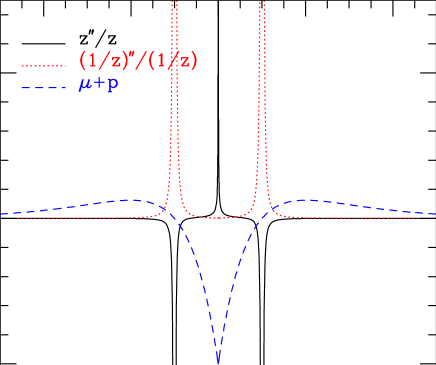
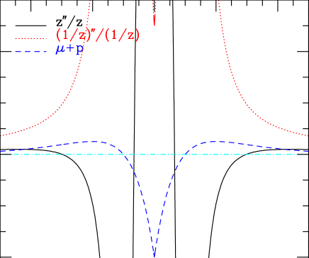
Figure 3: Evolutions of $z^{\prime\prime}/z$, $(1/z)^{\prime\prime}/(1/z)$, $\mu+p$ near the bounce [Panel (a)], and $\phi^{\prime}$, $\sigma^{\prime}$ [Panel (c)]. Panel (b) magnifies Panel (a) in vertical axis. In Panel (a), $(\mu+p)$ is plotted with $500$ times magnification. Panel (b) shows that $z^{\prime\prime}/z=0$ and $\mu+p=0$ occur at different epochs; $z^{\prime\prime}/z=0$ diverges at $\mu+p=0$ and at the bounce. These combinations appear in Eqs. (30)-(34) which we use to distinguish the adiabatic (curvature) and isocurvature modes, and the large and small scales. As these variables (except for $\sigma^{\prime}$) diverge or vanish some of our large-scale conditions or adiabatic conditions often become singular for very brief periods, see Figs. 4-6 and 10-15.

III.2 Equations in three different gauges

We will investigate the behaviors of $C$- and $d$-modes by following their evolutions from the collapsing phase to the expanding phase through our simple non-singular bounce model. In order to obtain numerical results, it is practically important to take a suitable temporal gauge condition. If we have the behavior of any one perturbation variable in any one gauge condition the rest of the variables even in the other gauge conditions can be algebraically derived using our equations in the gauge-ready form in Eqs. (17)-(23) and the gauge-invariant combinations; the latters are made from the gauge-transformation properties in Eq. (25), as in Eq. (26). We have chosen two gauge-invariant combinations $\varphi_{v}$ and $\varphi_{\chi}$ because of their conserved properties in the large-scale limit and popularity in the literature. We could not directly solve $\varphi_{v}$, however, because its equations show singular behavior near the bounce. We prefer a gauge condition that has no singular behavior through the bounce. We find several suitable gauge conditions and numerically solve them independently. The solution of any gauge-invariant variable should be the same independently of the gauge conditions. This naturally provides a way to check the numerical accuracy. For instance, $\varphi_{v}$ and $\varphi_{\chi}$ can be obtained from the solutions known in the uniform-$\sigma$ gauge ($\delta\sigma\equiv 0$) and in the zero-shear gauge ($\chi\equiv 0$) as

$$\varphi_{v}=\varphi_{\delta\sigma}-{a^{\prime}\over a}{\phi^{\prime}\delta\phi_{\delta\sigma}\over{\phi^{\prime}}^{2}-{\sigma^{\prime}}^{2}}=\varphi_{\chi}-{a^{\prime}\over a}{\phi^{\prime}\delta\phi_{\chi}-\sigma^{\prime}\delta\sigma_{\chi}\over{\phi^{\prime}}^{2}-{\sigma^{\prime}}^{2}},$$

$$\varphi_{\chi}=\varphi_{\delta\sigma}-{a^{\prime}\over a^{2}}\chi_{\delta\sigma}.$$ (43)

In the following we consider three different temporal gauge conditions. In each of these temporal gauge conditions, the temporal gauge degree of freedom is fixed completely, thus each of the variables in these gauge conditions has unique gauge-invariant counterparts, see hw4 . Thus, we can regard all the variables as gauge-invariant ones.

III.2.1 Uniform-curvature gauge

The uniform-curvature gauge takes $\varphi\equiv 0$ as the temporal gauge condition. This gauge condition is particularly suitable to handle quantum fluctuations generated during collapsing phase which will provide the initial seed fluctuations for the large-scale structures. This provides our initial conditions for numerical integration. From Eqs. (17)-(19),(22), and (23) we can derive

$$\delta\phi_{\varphi}^{\prime\prime}+2{a^{\prime}\over a}\delta\phi_{\varphi}^{\prime}+k^{2}\delta\phi_{\varphi}+a^{2}\left(V_{,\phi\phi}+{a^{2}\over{a^{\prime}}^{2}}{\phi^{\prime}}^{2}V+2{a\over a^{\prime}}V_{,\phi}\phi^{\prime}\right)\delta\phi_{\varphi}-a^{2}{a^{2}\over{a^{\prime}}^{2}}\sigma^{\prime}\left(V\phi^{\prime}+{a^{\prime}\over a}V_{,\phi}\right)\delta\sigma_{\varphi}$$

$$\quad={1\over a}\left[u^{\prime\prime}_{\delta\phi}+\left(k^{2}-{a^{\prime\prime}\over a}\right)u_{\delta\phi}\right]+\left[aV\left({a^{2}\over{a^{\prime}}^{2}}{\phi^{\prime}}^{2}+2{a\over a^{\prime}}{V_{,\phi}\over V}\phi^{\prime}+{V_{,\phi\phi}\over V}\right)u_{\delta\phi}-a{a\over{a^{\prime}}}\sigma^{\prime}V\left({a\over a^{\prime}}\phi^{\prime}+{V_{,\phi}\over V}\right)u_{\delta\sigma}\right]=0,$$ (44)

$$\delta\sigma_{\varphi}^{\prime\prime}+2{a^{\prime}\over a}\delta\sigma_{\varphi}^{\prime}+k^{2}\delta\sigma_{\varphi}-a^{2}{a^{2}\over{a^{\prime}}^{2}}{\sigma^{\prime}}^{2}V\delta\sigma_{\varphi}+a^{2}{a^{2}\over{a^{\prime}}^{2}}\sigma^{\prime}\left(V\phi^{\prime}+{a^{\prime}\over a}V_{,\phi}\right)\delta\phi_{\varphi}$$

$$\quad={1\over a}\left[u^{\prime\prime}_{\delta\sigma}+\left(k^{2}-{a^{\prime\prime}\over a}\right)u_{\delta\sigma}\right]+\left[-aV{a^{2}\over{a^{\prime}}^{2}}{\sigma^{\prime}}^{2}u_{\delta\sigma}+a{a\over{a^{\prime}}}\sigma^{\prime}V\left({a\over a^{\prime}}\phi^{\prime}+{V_{,\phi}\over V}\right)u_{\delta\phi}\right]=0,$$ (45)

where

$$u_{\delta\sigma}\equiv a\delta\sigma_{\varphi},\quad u_{\delta\phi}\equiv a\delta\phi_{\varphi}.$$ (46)

Away from the bounce, the effect of $\sigma$ is negligible, and we have the power law regime. From Eq. (11) we have $\phi^{\prime}\propto{a^{\prime}/a}$. Thus, we have

$$u^{\prime\prime}_{\delta\sigma}+\left(k^{2}-{a^{\prime\prime}\over a}\right)u_{\delta\sigma}=0,$$ (47)

$$u^{\prime\prime}_{\delta\phi}+\left(k^{2}-{a^{\prime\prime}\over a}\right)u_{\delta\phi}=0.$$ (48)

For a general $\lambda$ we have the following exact solutions

$$u_{(i)}=\sqrt{k|\eta|}[c_{1}(k)H_{\nu}^{(1)}(k|\eta|)+c_{2}(k)H_{\nu}^{(2)}(k|\eta|)],$$

$$\qquad\nu\equiv{3(w-1)\over 2(3w+1)}={3q-1\over 2(q-1)},$$ (49)

where $(i)=\delta\phi$ or $\delta\sigma$; $\lambda$ is related to $q$ and $w$ as in Eq. (11). If we take $\lambda=\sqrt{3}$, thus $w=0$ and $q={2/3}$, we have

$$u_{(i)} =\sqrt{2\over\pi}\Bigg{\{}-\left[\sin(|k\eta|)+{\cos(|k\eta|)\over|k\eta|}\right]\left[c_{1}(k)+c_{2}(k)\right]$$ (50)

$$+i\left[\cos(|k\eta|)-{\sin(|k\eta|)\over|k\eta|}\right]\left[c_{1}(k)-c_{2}(k)\right]\Bigg{\}}.$$

These will provide the initial seed fluctuations. Identification of these classical solutions with the initial fluctuations generated from the quantum fluctuations will be considered in Sec. V. The equations in this gauge, however, show the singular behavior as the background passes through the bounce. Thus, in order to follow the evolution numerically we need to use other gauge conditions which are well-defined throughout the bounce.

III.2.2 Uniform-$\sigma$ gauge

The uniform-$\sigma$ gauge takes $\delta\sigma\equiv 0$ as the temporal gauge condition. Authors of AW used this gauge condition for their numerical calculation. From Eqs. (17), (19), (20), (22), and (23) we have

$$\delta\phi_{\delta\sigma}^{\prime\prime}+2{a^{\prime}\over a}\delta\phi_{\delta\sigma}^{\prime}+a^{2}V_{,\phi\phi}\delta\phi_{\delta\sigma}+k^{2}\delta\phi_{\delta\sigma}+2a^{2}V_{,\phi}\alpha_{\delta\sigma}=0,$$ (51)

$$\varphi_{\delta\sigma}^{\prime\prime}+2{a^{\prime}\over a}\varphi_{\delta\sigma}^{\prime}+{1\over 2}\left({\phi}^{\prime}\delta\phi_{\delta\sigma}^{\prime}-a^{2}V_{,\phi}\delta\phi_{\delta\sigma}\right)-a^{2}V\alpha_{\delta\sigma}-{a^{\prime}\over a}\alpha_{\delta\sigma}^{\prime}=0,$$ (52)

$$\alpha_{\delta\sigma}^{\prime}-3\varphi_{\delta\sigma}^{\prime}+{k^{2}\over a}\chi_{\delta\sigma}=0,$$ (53)

$$\chi_{\delta\sigma}^{\prime}+{a^{\prime}\over a}\chi_{\delta\sigma}-a(\alpha_{\delta\sigma}+\varphi_{\delta\sigma})=0.$$ (54)

Thus, in this gauge we solve sixth-order differential equations. Although, this set of sixth-order differential equations can be easily reduced to a fourth-order differential equation, in order to follow numerically the evolution of perturbations through the bounce without singular behavior these sixth-order differential equations are preferred. In order to provide initial conditions for $\alpha_{\delta\sigma}$ and $\chi_{\delta\sigma}$ we use the following constraint equations

$$\alpha_{\delta\sigma}={a\over a^{\prime}}\left(\varphi^{\prime}_{\delta\sigma}+{1\over 2}\phi^{\prime}\delta\phi_{\delta\sigma}\right),$$ (55)

$$\chi_{\delta\sigma}=a\Bigg{\{}{a\over a^{\prime}}\varphi_{\delta\sigma}-{3\over 2}{1\over k^{2}}\phi^{\prime}\delta\phi_{\delta\sigma}-{1\over 2k^{2}}{a\over a^{\prime}}\left[\phi^{\prime}\delta\phi_{\delta\sigma}^{\prime}-({\phi^{\prime}}^{2}-{\sigma^{\prime}}^{2})\alpha_{\delta\sigma}+a^{2}V_{,\phi}\delta\phi_{\delta\sigma}\right]\Bigg{\}},$$ (56)

which follow from Eqs. (17) and (19) and Eqs. (18) and (19), respectively. Since the initial conditions are provided in the uniform-curvature gauge, in order to construct initial conditions for the variables in the uniform-$\sigma$ gauge it is convenient to have

$$\delta\phi_{\delta\sigma}=\delta\phi_{\varphi}-{\phi^{\prime}\over\sigma^{\prime}}\delta\sigma_{\varphi},\quad{\delta\phi}^{\prime}_{\delta\sigma}={\delta\phi}^{\prime}_{\varphi}+a^{2}V_{,\phi}{\delta\sigma_{\varphi}\over\sigma^{\prime}}-{\phi^{\prime}\over\sigma^{\prime}}\delta\sigma^{\prime}_{\varphi},$$

$$\varphi_{\delta\sigma}=-{a^{\prime}\over a}{\delta\sigma_{\varphi}\over\sigma^{\prime}},\quad\varphi^{\prime}_{\delta\sigma}=-a^{2}V{\delta\sigma_{\varphi}\over\sigma^{\prime}}-{a^{\prime}\over a}{{\delta\sigma}^{\prime}_{\varphi}\over\sigma^{\prime}}.$$ (57)

From Eq. (39) we can read the initial conditions for the $C$- and $d$-modes of $\varphi_{v}$. In order to have the $C$- and $d$-mode decomposition, it is necessary to satisfy the large-scale and the adiabatic conditions. From Eq. (30) the adiabatic condition implies ${\delta\sigma/\dot{\sigma}}={\delta\phi/\dot{\phi}}$. From this, we construct $C$- and $d$-modes of $\varphi_{v}$ and the related variables in the uniform-$\sigma$ gauge. Thus, the initial conditions for the $C$-mode and $d$-mode are, respectively

$$C{\rm-mode}:\delta\phi_{\delta\sigma}=0,\quad{\delta\phi^{\prime}_{\delta\sigma}}=0,\quad\varphi_{\delta\sigma}=C,\quad{\varphi^{\prime}_{\delta\sigma}}=0,$$

$$d{\rm-mode}:\delta\phi_{\delta\sigma}=0,\quad{\delta\phi^{\prime}_{\delta\sigma}}=0,\quad\varphi_{\delta\sigma}=d,\quad{\varphi^{\prime}_{\delta\sigma}}=-{3\over\eta}d.$$ (58)

It is important to notice, however, that these are initial conditions for the $C$- and $d$-modes in an ideal situation when the large-scale and the adiabatic conditions are satisfied exactly. Since both of these conditions are not satisfied exactly in the two-component medium, we have to find precise $C$- and $d$-mode initial conditions which have correct behaviors in the initial phase and preferably throughout the bounce.

In Sec. IV we will present evolution of perturbations under such precise initial conditions (we call these ‘our initial $C$- and $d$-mode’ initial conditions) which preserve the $C$- and $d$-mode natures throughout the bounce; we will show that, under this evolution, the isocurvature perturbation is not excited near the bounce. We will also present the perturbation behaviors under the naive initial conditions based on the analytic solutions in an ideal situation in Eq. (58) (we call these ‘analytic $C$- and $d$-mode’ initial conditions) which fail to produce the desired results. In short, the initial conditions in Eq. (58), in fact, correspond to mixtures of the $C$- and $d$-modes in the initial phase, and lead to loss of these mode identities as the evolution proceeds through the bounce; under this evolution, the isocurvature perturbation is also excited near the bounce, see Sec. IV.

III.2.3 Zero-shear gauge

The zero-shear gauge takes $\chi\equiv 0$ as the temporal gauge condition. From Eqs. (17), (19), (20), (22), and (23) we have

$$\varphi^{\prime}_{\chi}=-{a^{\prime}\over a}\varphi_{\chi}-{1\over 2}(\phi^{\prime}\delta\phi_{\chi}-\sigma^{\prime}\delta\sigma_{\chi}),$$ (59)

$$\delta\phi_{\chi}^{\prime\prime}+2{a^{\prime}\over a}\delta\phi_{\chi}^{\prime}+a^{2}V_{,\phi\phi}\delta\phi_{\chi}+k^{2}\delta\phi_{\chi}=4\phi^{\prime}\left[{a^{\prime}\over a}\varphi_{\chi}+{1\over 2}(\phi^{\prime}\delta\phi_{\chi}-\sigma^{\prime}\delta\sigma_{\chi})\right]+2a^{2}V_{,\phi}\varphi_{\chi},$$ (60)

$$\delta\sigma_{\chi}^{\prime\prime}+2{a^{\prime}\over a}\delta\sigma_{\chi}^{\prime}+k^{2}\delta\sigma_{\chi}=4\sigma^{\prime}\left[{a^{\prime}\over a}\varphi_{\chi}+{1\over 2}(\phi^{\prime}\delta\phi_{\chi}-\sigma^{\prime}\delta\sigma_{\chi})\right].$$ (61)

In order to construct the initial conditions in this gauge we need the following relations

$$\delta\phi_{\chi}=\delta\phi_{\delta\sigma}-{{\phi^{\prime}}\over a}\chi_{\delta\sigma},\quad\delta\sigma_{\chi}=-{{\sigma^{\prime}}\over a}\chi_{\delta\sigma},\quad\delta\phi_{\chi}^{\prime}=\delta\phi_{\delta\sigma}^{\prime}+3{a^{\prime}\over a^{2}}\phi^{\prime}\chi_{\delta\sigma}+aV_{,\phi}\chi_{\delta\sigma}-{\phi^{\prime}\over a}\chi_{\delta\sigma}^{\prime},$$

$$\delta\sigma_{\chi}^{\prime}=3{a^{\prime}\over a^{2}}\sigma^{\prime}\chi_{\delta\sigma}-{\sigma^{\prime}\over a}\chi_{\delta\sigma}^{\prime},\quad\varphi_{\chi}=\varphi_{\delta\sigma}-{a^{\prime}\over a^{2}}\chi_{\delta\sigma},$$ (62)

where

$$\chi_{\delta\sigma} = {a^{2}\over a^{\prime}}\Bigg{\{}\varphi_{\delta\sigma}+{1\over 2k^{2}}\Bigg{[}{a\over a^{\prime}}\left({\phi^{\prime}}^{2}-{\sigma^{\prime}}^{2}\right){\varphi}^{\prime}_{\delta\sigma}-\phi^{\prime}\delta\phi^{\prime}_{\delta\sigma}-a^{2}\left(V_{,\phi}+{a\over a^{\prime}}\phi^{\prime}V\right)\delta\phi_{\delta\sigma}\Bigg{]}\Bigg{\}},$$

$$\chi^{\prime}_{\delta\sigma} = -{a^{\prime}\over a}\chi_{\delta\sigma}+{a^{2}\over a^{\prime}}\varphi^{\prime}_{\delta\sigma}+a\varphi_{\delta\sigma}+{a^{2}\over 2a^{\prime}}\phi^{\prime}\delta\phi_{\delta\sigma}.$$ (63)

Relations in Eq. (63) follow from Eqs. (54)-(56). Equations in this gauge also behave well throughout the bounce. Numerical results in this gauge condition should coincide with the ones from the uniform-$\sigma$ gauge for any gauge-invariant combination which provides a self-consistent numerical check.

III.3 Tensor-type perturbations

The tensor-type perturbations correspond to the gravitational waves. It is described by Eq. (24). The scalar fields do not directly contribute to the tensor-type perturbations, i.e., $\Pi_{\alpha\beta}\equiv 0$. Equation (24) becomes

$${1\over a^{3}}\left(a^{3}\dot{C}_{\alpha\beta}^{(t)}\right)^{\cdot}+{k^{2}\over a^{2}}C_{\alpha\beta}^{(t)}$$

$$\qquad={1\over a^{3}}\left[\hat{v}_{t}^{\prime\prime}-\left({a^{\prime\prime}\over a}-k^{2}\right)\hat{v}_{t}\right]=0,$$ (64)

where $\hat{v}_{t}\equiv aC^{(t)}_{\alpha\beta}$. Notice the similarity of this equation compared with Eq. (30) for $\varphi_{v}$. In the large-scale limit we have

$$C_{\alpha\beta}^{(t)}(k,\eta)=\bar{C}_{\alpha\beta}(k)+\bar{d}_{\alpha\beta}(k)\int^{\eta}{1\over a^{2}}d\eta,$$ (65)

where $\bar{C}_{\alpha\beta}$ and $\bar{d}_{\alpha\beta}$ are integration constants. To the next order in the large-scale expansion we have

$$C_{\alpha\beta}^{(t)}(k,\eta) = \bar{C}_{\alpha\beta}(k)\Bigg{\{}1+k^{2}\Bigg{[}\int^{\eta}\left({a^{2}}\int^{\eta}{1\over a^{2}}d\eta\right)d\eta$$ (66)

$$-\int^{\eta}{1\over a^{2}}d\eta\int^{\eta}{a^{2}}d\eta\Bigg{]}\Bigg{\}}+\bar{d}_{\alpha\beta}(k)\Bigg{\{}\int^{\eta}{1\over a^{2}}d\eta$$

$$+k^{2}\Bigg{[}\int^{\eta}{a^{2}}\left(\int^{\eta}{1\over a^{2}}d\eta\right)\left(\int^{\eta}{1\over a^{2}}d\eta\right)d\eta$$

$$-\left(\int^{\eta}{1\over a^{2}}d\eta\right)\int^{\eta}\left({a^{2}}\int^{\eta}{1\over a^{2}}d\eta\right)d\eta\Bigg{]}\Bigg{\}}.$$

The above solutions can be compared with Eqs. (39),(41) for $\varphi_{v}$.

For

$${a^{\prime\prime}\over a}={n_{g}\over\eta^{2}},\quad n_{g}\equiv{q(2q-1)\over(1-q)^{2}},$$ (67)

Eq. (64) has an exact solution

$$C_{\alpha\beta}^{(t)}(k,\eta) = {\sqrt{|\eta|}\over a}\Big{[}\tilde{c}_{1\alpha\beta}({k})H_{\nu_{g}}^{(1)}(k|\eta|)$$ (68)

$$+\tilde{c}_{2\alpha\beta}({k})H_{\nu_{g}}^{(2)}(k|\eta|)\Big{]},$$

$$\nu_{g}\equiv{1\over 2}{3q-1\over 1-q}.$$

For $q=2/3$, we have

$$C_{\alpha\beta}^{(t)}(k,\eta) = {1\over a}\sqrt{2\over\pi k}\Bigg{\{}\Bigg{[}-\cos(|k\eta|)+{\sin(|k\eta|)\over|k\eta|}\Bigg{]}\Big{[}\tilde{c}_{1\alpha\beta}({k})$$ (69)

$$+\tilde{c}_{2\alpha\beta}({k})\Big{]}-i\Big{[}\sin(|k\eta|)+{\cos(|k\eta|)\over|k\eta|}\Big{]}$$

$$\times\Big{[}\tilde{c}_{1\alpha\beta}({k})-\tilde{c}_{2\alpha\beta}({k})\Big{]}\Bigg{\}}.$$

IV Numerical results

IV.1 Scalar-type perturbations

IV.1.1 Our $C$- and $d$-modes

In Figs. 4(a), 4(b), 6(a), and 6 (b), we present evolutions of ‘our $C$- and $d$-modes’. These are based on our $C$- and $d$-mode initial conditions presented in Table 2. These figures apparently show that evolutions away from the bounce coincide with the known behaviors of the $C$- and $d$-modes based on the large-scale analytic solutions in Eqs. (39) and (40). These analytic solutions are valid when both the large-scale conditions and the adiabatic conditions are satisfied.

In Fig. 5 we examine the large-scale conditions using Eq. (36). Figure 5(a) apparently shows that the large-scale condition for $\varphi_{v}$ is sharply broken four times near the bounce at $z^{\prime\prime}/z=0$, see Fig. 3. Despite these sharp divergences in our large-scale condition, we argue that these do not have physical impact on interpreting the $C$- and $d$-mode natures of $\varphi_{v}$ in Figs. 4(a) and 6(a). This is because our large-scale condition is sharply broken as the $z^{\prime\prime}/z$ term in Eq. (30) crosses zero, thus becomes smaller than $k^{2}$-term, for very brief time intervals, see Fig. 3. Figure 5(b) shows that the large-scale condition is well satisfied for $\varphi_{\chi}$. The large-scale conditions involve only the background evolution and the wavenumber. Thus, the same large-scale condition applies to both $C$- and $d$-modes independently of the initial conditions for perturbations.

In Figs. 4(c), 4(d), 6(c), and 6(d) we examine adiabatic conditions using Eq. (37). All these figures show that the adiabatic conditions are sharply broken near the bounce. These occur at $z^{\prime\prime}/z=0$, $\mu+p=0$, or $\varphi_{\chi}=0$. Despite these sharp divergences in our adiabatic conditions, we argue that these do not have physical impact on interpreting the $C$- and $d$-mode natures of $\varphi_{v}$ in Figs. 4(a) and 6(a). We have two reasons. First, $\varphi_{v}$ in Figs. 4(a) and 6(a) shows that the $C$- and $d$-mode natures are preserved away from the bounce. Second, later in Figs. 12 and 13 we will show that for our $C$- and $d$-modes the isocurvature perturbation is not excited near the bounce.

Compared with the above sharp spikes in the adiabatic conditions, Fig. 6(c) shows that the adiabatic condition for $\varphi_{v}$ is severely broken near the bounce region. Remember that the $d$-mode of $\varphi_{v}$ in Eq. (39) is higher order in the large-scale expansion compared with the same mode of $\varphi_{\chi}$ in Eq. (40); this happens because the leading order large-scale solution of the $d$-mode of $\varphi_{v}$ has canceled out, see Eqs. (28) and (42). Thus, as the $d$-mode of $\varphi_{v}$ is $(k/aH)^{2}$-factor smaller than the $d$-mode of $\varphi_{\chi}$ we could have such a breakdown in Fig. 6(c) without affecting the $d$-mode nature of $\varphi_{v}$ before and after the bounce.

Based on the above arguments, we suggest that ‘our $C$- and $d$-mode initial conditions’ in Table 2 produce the proper $C$- and $d$-modes which are valid throughout the bounce, as presented in Figs. 4(a), 4(b), 6(a), and 6(b). In order to obtain these numerical results producing proper $C$- and $d$-mode decomposition, we have to find the precise initial condition; the method will be explained in Sec. IV.1.3.

In an ideal situation we may use the initial conditions of $\varphi_{v}$ and $\varphi_{\chi}$ in Eq. (58) which are valid when the large-scale and the adiabatic conditions are satisfied exactly; these initial conditions are summarized in Table 3, and numerical results will be presented in Sec. IV.1.2. Since these two conditions are not exactly satisfied in reality, we have to find more accurate initial conditions which allow the correct $C$- and $d$-mode behavior at the initial phase, and preferably throughout the bounce. The correct initial conditions we found are presented in Table 2, and the numerical results are presented in Figs. 4 and 6.

As noted in Sec. III.2, we solve numerically two independent sets of equations based on two different temporal gauge conditions: these are Eqs. (51)-(54) in the uniform-$\sigma$ gauge, and Eqs. (59)-(61) in the zero-shear gauge. We derive initial conditions for variables in the zero-shear gauge using relations between the uniform-$\sigma$ gauge and the zero-shear gauge in Eq. (62). Any gauge-invariant combination of variables should show the same behavior independently of the gauge conditions we took. This provides a numerical check of the accuracy of our integration. Although evolutions of $\varphi_{v}$ and $\varphi_{\chi}$ in Figs. 4 and 6 sometimes show singular behaviors near the bounce, these are due to the singular behavior of background variables multiplied to form these gauge-invariant combinations, e.g., see Eq. (43). In Figs. 7 and 8 we show that during our numerical integration the original variables used in the integration behave smoothly.

In Figure 9, we show the $C$-mode evolution of $\varphi_{v}$ and $\varphi_{\chi}$ for a different scale which enter the horizon at later epoch; here we set $k=10^{-6}$ whereas in other figures we used $k=0.0005$, and the initial conditions differ from the other figures.

Our results in Figs. 4 and 6 show that by taking the correct initial conditions representing the $C$- and $d$-modes for $\varphi_{v}$ and $\varphi_{\chi}$, the identities of $C$- and $d$-modes remain valid throughout the bounce. That is, the $C$-mode remains as the $C$-mode throughout the bounce, and similarly for the $d$-mode. Although in the collapsing phase it is the $d$-mode which is relatively growing, it decays away in the expanding phase. Thus, if we are interested in the relatively growing mode in the final expanding phase we have to consider the $C$-mode even in the collapsing phase. This is one of the major points we have emphasized in our previous works based on analytic arguments in hw1 ; hw2 ; HN-bounce , and here we confirm it by using the numerical integration based on a specific bounce model.

Table 2: The initial conditions which give the precise (thus, correct) $C$- and $d$-mode behaviors in both collapsing and expanding phases away from the bounce. We call these ‘our $C$- and $d$mode initial conditions, or simply ‘our $C$- and $d$-modes. We take $k=0.0005$ and the initial $\eta=-500$. The numerical results based on these initial conditions are presented in Figs. 4-8.

variable	C-mode	d-mode
$\delta\phi_{\delta\sigma}$	$-$7.8058229814554E$-$06	$-$1.5568456514629E$+$03
$\delta\phi_{\delta\sigma}^{\prime}$	4.6325084877449E$-$08	8.9724639867256E+00
$\varphi_{\delta\sigma}$	5.4370235008682E$-$06	$-$8.9884525573535E$+$02
$\varphi_{\delta\sigma}^{\prime}$	2.7003984444483E$-$08	5.1802544967425E$+$00
$\varphi_{v}$	9.9439752296909E$-$06	1.0015746283898E$-$05
$\varphi_{v}^{\prime}$	2.5769163366172E$-$10	5.8225396948330E$-$08

Figure 4: Evolutions of our $C$-modes for $\varphi_{v}$ and $\varphi_{\chi}$, and the adiabatic conditions; the large-scale conditions are presented in Fig. 5. Panels (a) and (b) show the behaviors of our $C$-modes for $\varphi_{v}$ and $\varphi_{\chi}$. We use the initial conditions in Table. 2. Panels (c) and (d) show the adiabatic conditions for $\varphi_{v}$ and $\varphi_{\chi}$, respectively; for $\varphi_{v}$ and $\varphi_{\chi}$ we plot the LHSs of Eq. (37). Panel (c) shows that the adiabatic condition for $\varphi_{v}$ is broken by sharp peaks (divergences) six times near the bounce; we can show that the four sharp peaks at the outer edge and the inner edge surrounding the bounce are caused by $z^{\prime\prime}/z=0$, and the other two sharp peaks in the middle are caused by $\mu+p=0$. The adiabatic condition for $\varphi_{\chi}$ in Panel (d) also shows two sharp peaks just before the bounce because $\varphi_{\chi}$ crosses zero at these two points; see Eq. (37) and Fig. 7(f) which shows evolution of $\varphi_{\chi}$ in a linear scale. Later, in Fig. 12 we will show that the isocurvature perturbation is not affected by the presence of these sharp peaks in the adiabatic condition and in the large-scale condition; the latter will be presented in Fig. 5. Based on this observation and the physical behaviors of the curvature variables throughout the bounce, we suggest that such peaks do not have physical impact on the $C$- and $d$-mode natures of the perturbation. Panel (a) shows a spike in the evolution of $\varphi_{v}$ just after the bounce; it actually have two spikes at $\mu+p=0$, see Eq.  (43) and Fig. 7. Away from the bounce we have $\varphi_{\chi}=(3/5)\varphi_{v}$ which is the well known ratio for $w=0$ background.

Figure 5: Large-scale conditions for $\varphi_{v}$ and $\varphi_{\chi}$. Panels (a) and (b) show the large-scale conditions for $\varphi_{v}$ and $\varphi_{\chi}$ equations; for $\varphi_{v}$ and $\varphi_{\chi}$ we plot $k^{2}/(z^{\prime\prime}/z)$, and $k^{2}/[(1/z)^{\prime\prime}/(1/z)]$, respectively. As the large-scale conditions involve only the background evolution and the wavenumber, the same large-scale conditions apply to both $C$- and $d$-modes independently of the initial condition. Panel (a) shows that the large-scale condition for $\varphi_{v}$ is broken four times by sharp peaks (divergences) near the bounce. These divergences occur at $z^{\prime\prime}/z=0$. As explained in Fig. 4, as the isocurvature perturbation is not affected by the presence of these sharp peaks in the large-scale condition, such peaks are not supposed to have physical impact on interpreting the $C$- and $d$-mode natures.

Figure 6: Evolutions of our $d$-modes for $\varphi_{v}$ and $\varphi_{\chi}$, and the adiabatic conditions; the large-scale conditions are presented in Fig. 5. Panels (a) and (b) show the behaviors of $d$-modes for $\varphi_{v}$ and $\varphi_{\chi}$, respectively. We use the initial conditions in Table 2. Both $\varphi_{v}$ and $\varphi_{\chi}$ cross zero at the bounce, see Figs. 8(d) and 8(e) which show the evolution in linear scale. $\varphi_{v}$ diverges twice near the bounce at $\mu+p=0$, see Eq. (43) and Fig. 8(d). Panels (c) and (d) show the adiabatic conditions for $\varphi_{v}$ and $\varphi_{\chi}$. Although, the adiabatic condition for $\varphi_{v}$ equation is severely broken near the bounce, we interpret this happens because the $d$-mode of $\varphi_{v}$ is $(k/aH)^{2}$-order higher in the large-scale expansion compared with the same mode of $\varphi_{\chi}$, i.e, the leading order $d$-mode of $\varphi_{v}$ has been canceled out; see Eqs. (39) and (40), or Eqs. (41) and (42). Panel (c) also shows four sharp peaks (divergences) near the bounce which are caused by $z^{\prime\prime}/z=0$; compared with Fig. 4(c), the two sharp peaks potentially caused by $\mu+p=0$ disappeared because the $d$-mode of $\varphi_{v}$ diverges in proportion to $1/(\mu+p)$, e.g., see Eq. (39) and Panel (a). The adiabatic condition for $\varphi_{\chi}$ has one sharp peak at the bounce because $\varphi_{\chi}$ crosses zero at this points; see Eq. (37) and Fig. 8(e). As explained in Fig. 4, the isocurvature perturbation is not affected by the presence of these sharp peaks in the adiabatic condition, and the $d$-mode before the bounce remains as the $d$-mode after the bounce. Thus, such peaks do not have physical impact on the $d$-mode natures of the perturbations.

Figure 7: The raw behaviors of gauge-invariant variables numerically solved using Eqs. (51)-(54) for $C$-modes of $\varphi_{v}$ and $\varphi_{\chi}$. Panels (a)-(c),(e) show that the variables we used in numerical integration behave smoothly throughout the evolution. We obtain the behaviors of $\varphi_{v}$ and $\varphi_{\chi}$ in Panels (d) and (f) using Eq. (43). Panel (c) magnifies Panel (b) near the bounce region. This figure explains why we have only one sharp spike after the bounce visible in Panel (d) and Fig. 4(a); the spikes are caused by vanishing $\mu+p$ in Eq. (43). The arrows indicate the epochs where $\mu+p=0$.

Figure 8: The same as Fig. 7, now, for the $d$-mode. Panels (a)-(c) show that the variables we used in numerical integration behave smoothly throughout the evolution.

Figure 9: Long term evolution of the $C$-mode. This figure shows the evolutions of $C$-modes using $k=10^{-6}$. The inset figure shows that the scale becomes subhorizon near $\log{(a/a_{min})}=10$. Both $\varphi_{v}$ and $\varphi_{\chi}$ begin oscillations as the scale comes inside the (visual) horizon. In a realistic situation, the horizon crossing of relevant cosmic scales should occur long after the bounce.

IV.1.2 Analytic $C$- and $d$-modes

In Figs. 10(a), 10(b), 11(a), and 11(b) we present some generic behaviors of imprecisely imposed $C$- and $d$-mode initial conditions. Unless we set up initial conditions precisely as in ‘our $C$- and $d$-modes’ presented in Table 2, it is very likely that the curvature perturbations behave similar to the ones in Figs. 10(a), 10(b), 11(a), and 11(b). What is actually presented in these figures is based on ‘analytic $C$- and $d$-mode’ initial conditions in Table 3. These initial conditions are based on the large-scale limit solutions of adiabatic perturbation in Eqs. (39) and (40). Thus, these are valid for an ideal situation assuming exact validity of the adiabatic condition and the large-scale limit.

In Figs. 10(c), 10(d), 11(c), and 11(d) we present the adiabatic conditions. The large-scale conditions are the same as in Fig. 5. Detailed descriptions of the evolutions and the adiabatic conditions can be found in the figure captions. Sharp spikes away from the bounce in the adiabatic conditions in Figs. 10(c), 10(d), and 11(d) occur at $\varphi_{v}=0$ or $\varphi_{\chi}=0$ which can be identified in Figs. 10(a), 10(b), and 11(b). The curvature perturbations vanish at these points as the dominating mode changes between the $C$-mode and the $d$-mode. Sharp spikes at the bounce in Figs. 10(d) and 11(d) occur because $\varphi_{\chi}=0$ at the bounce. Even in our $d$-mode case we have $\varphi_{\chi}=0$ at the bounce, see Fig. 6. Figures 10(b) and 11(b) are effectively the same; although we call Fig. 10(b) an analytic $C$-mode, apparently, the initial condition is dominated by the $d$-mode from the beginning.

The adiabatic conditions for $\varphi_{v}$ in 10(c) and 11(c) are severely broken near the bounce. Evolutions of $\varphi_{v}$ in Figs. 10(a) and 11(a) also show switching of the $d$-mode before the bounce into the $C$-mode after the bounce. Furthermore, Figures 12 and 13 show that, for the analytic $C$- and $d$-modes, the isocurvature perturbation is significantly excited at the bounce. Based on these observations we conclude that we cannot trace the $C$-modes after the bounce to the $d$-modes before the bounce in Figs. 10(a) and 11(a). This conclusion should be compared with the one made in our $d$-mode case. Although, the adiabatic condition for our $d$-mode is also severely broken near the bounce [see Fig. 6(c)], there we have argued how this could happen for the $d$-mode of $\varphi_{v}$ without affecting the $d$-mode nature before and after the bounce. In our $d$-mode case, Fig. 6(a) shows that the $d$-mode nature is preserved before and after the bounce, and Fig. 13 shows that the isocurvature perturbation is not excited near the bounce.

The evolutions show that each mode is soon dominated by the relatively growing mode (the $d$-mode in a collapsing phase, and the $C$-mode in an expanding phase are the relatively growing). In fact, these analytic initial conditions correspond to mixtures of our precise $C$- and $d$-mode initial conditions. Based on these observations we conclude that we cannot trace the final $C$-modes after the bounce in all these figures to the ones provided initially.

Table 3: The analytic initial conditions in Eq. (58). This initial condition is valid for an ideal situation assuming exact validity of the adiabatic condition, and taking the leading order solution in large-scale expansion presented in Eqs. (39) and (40). We call these ‘analytic $C$- and $d$-mode initial conditions’, or simply ‘analytic $C$- and $d$-modes’. We take $k=0.0005$ and the initial $\eta=-500$. The numerical results based on these initial conditions are presented in Figs. 10 and 11.

variable	C-mode	d-mode
$\delta\phi_{\delta\sigma}$	0.	0.
$\delta\phi_{\delta\sigma}^{\prime}$	0.	0.
$\varphi_{\delta\sigma}$	1.0E$-$05	1.0E$-$05
$\varphi_{\delta\sigma}^{\prime}$	0.	$-$3./$\eta\times\varphi_{\delta\sigma}$
$\varphi_{v}$	1.0E$-$05	1.0E$-$05
$\varphi_{v}^{\prime}$	0.	$-$3./$\eta\times\varphi_{v}$

Figure 10: Evolutions under the ‘analytic $C$-mode’ initial condition in Table 3 which is valid for an ideal situation based on an analytic solution. This figures is the same as Fig. 4, now for an analytic $C$-mode initial condition. Panels (a) and (b) show evolutions of $\varphi_{v}$ and $\varphi_{\chi}$. Panels (c) and (d) show adiabatic conditions for $\varphi_{v}$ and $\varphi_{\chi}$. The large-scale conditions are the same as in Fig. 5. Compared with ‘our $C$-mode’ presented in Fig. 4, which shows that the $C$-mode nature is maintained before and after the bounce, the present ‘analytic $C$-mode’ leads to mixed behaviors of the $C$- and $d$-modes. In the present case, the initial condition in Table 3 corresponds to a mixture of our precise $C$- and $d$-modes presented in Figs. 4 and 6, respectively. Panels (c) and (d) show that the present initial conditions lead to failures of the adiabatic conditions both for $\varphi_{v}$ and $\varphi_{\chi}$ during the evolution. Two sharp spikes away from the bounce in Panels (c) and (d) are caused because the curvature variables $\varphi_{v}$ and $\varphi_{\chi}$ vanish as the dominating mode switches between the $C$-mode and the $d$-mode, see Panels (a) and (b). The sharp spike at the bounce in Panel (d) is caused because $\varphi_{\chi}$ vanishes at the bounce; apparently, the behavior of $\varphi_{\chi}$ shows its $d$-mode nature before and after the bounce, thus vanishes at $H=0$, see Eq. (40). As in our $C$-mode in Fig. 4, such a sharp peak does not affect the $d$-mode nature of $\varphi_{\chi}$ at the bounce. The adiabatic condition for $\varphi_{v}$ in Panel (c), however, is severely broken near the bounce. The evolution of $\varphi_{v}$ in Panel (a) also shows switching of the $d$-mode before the bounce into the $C$-mode after the bounce. Furthermore, later in Fig. 12 we will show that, for the analytic $C$-mode, the isocurvature perturbation is significantly excited at the bounce. Based on these observations we conclude that we cannot trace the $C$-mode after the bounce to the one provided initially.

Figure 11: The same figures as in Fig. 10, now for the analytic $d$-mode initial condition in Table 3. Compared with ‘our $d$-mode’ presented in Fig. 6, which show that the $d$-mode nature is maintained before and after the bounce, the present ‘analytic $d$-mode’ leads to mixed behaviors of the $C$- and $d$-modes. In the present case, the initial condition in Table 3 corresponds to a mixture of our precise $C$- and $d$-modes presented in Figs. 4 and 6, respectively. Panels (c) and (d) show that the present initial conditions lead to failures of the adiabatic conditions both for $\varphi_{v}$ and $\varphi_{\chi}$ during the evolution. One sharp spike away from the bounce in Panel (d) is caused because $\varphi_{\chi}$ vanishes as the dominating mode switches from $d$-mode to $C$-mode, see Panel (b). As explained in Fig. 10, the sharp spike at the bounce in Panel (d), caused by vanishing $\varphi_{\chi}$ at $H=0$, does not affect the $d$-mode nature of $\varphi_{\chi}$ at the bounce. As in Fig. 10, the adiabatic condition for $\varphi_{v}$ in Panel (c) is severely broken near the bounce. The evolution of $\varphi_{v}$ in Panel (a) also shows switching of the $d$-mode before the bounce into the $C$-mode after the bounce. Later in Fig. 13 we will show that, for the analytic $d$-mode, the isocurvature perturbation is significantly excited at the bounce. Based on these observations we conclude that we cannot trace the $d$-mode after the bounce to the one provided initially. The adiabatic condition for $\varphi_{v}$ is also severely broken for ‘our $d$-mode’ in Fig. 6. In the case of our $d$-mode, in Fig. 6 we have argued that this happens because the $d$-mode of $\varphi_{v}$ is $(k/aH)^{2}$-order smaller than the $d$-mode of $\varphi_{\chi}$, thus quite small, see Eq. (39). Furthermore, in the case of our $d$-mode the isocurvature perturbation is not excited near the bounce, despite the apparent breakdown of the adiabatic condition for $\varphi_{v}$, see Fig. 13.

Figure 12: Evolutions of the isocurvature perturbation variable $S_{\phi\sigma}$ for ‘our $C$-mode’ (solid line) and the ‘analytic $C$-mode’ (dotted line). Panel (b) magnifies Panel (a) near the bounce. Panel (c) shows Panel (a) in logarithmic scale. The sharp divergences at the bounce occur because we have $\dot{\phi}=0$ at the bounce. For our $C$-mode, $S_{\phi\sigma}$ nearly vanishes near $\log{(a/a_{min})}\simeq-.2$; this is because we have found our $C$-mode initial condition beginning at this epoch, see the text for explanation. Although Figs. 4(c) and (d) show that the adiabatic conditions for our $C$-modes of $\varphi_{v}$ and $\varphi_{\chi}$ are broken by sharp peaks near the bounce, the above figures show that the isocurvature variable $S_{\phi\sigma}$ show smooth behavior near the bounce. As explained in Fig. 4, such sharp divergences occur because we have $\mu+p=0$ near the bounce and $\varphi_{\chi}$ crosses zero twice near the bounce, see Fig. 4(b). In case of the analytic $C$-mode, Figs. 10(c) and (d) show that the adiabatic conditions are severely broken near the bounce, and are sharply broken in two places away from the bounce. As explained in Fig. 10, the two sharp spikes away from the bounce occur because of the change in dominating mode between $C$-mode and $d$-mode, where the curvature variables $\varphi_{v}$ or $\varphi_{\chi}$ vanish. The above figures show that for the analytic $C$-mode the isocurvature variable significantly changes its behavior at the bounce. Based on these behaviors, we argue that for our $C$-mode initial condition although the adiabatic conditions are broken by sharp peaks near the bounce, because the isocurvature perturbation shows the smooth behavior, the isocurvature perturbation does not give physical impact on the adiabatic nature of our $C$-mode throughout the bounce. Thus, although our $C$-mode initial condition shows apparently non-vanishing isocurvature mode (see Table 2), we argue that our $C$-mode initial condition keeps the adiabatic nature throughout the bounce. On the other hand, for the analytic $C$-mode, the adiabatic conditions are severely broken near the bounce, and the isocurvature perturbation shows sharp change at the bounce. Thus, we argue that the isocurvature perturbation gives physical impact on the adiabatic nature of the analytic $C$-mode; this analytic $C$-mode is based on an initial condition with ‘precise’ adiabatic condition (see Table 3). That is, for the analytic $C$-mode, although the initial condition is imposed assuming the adiabatic condition is exactly met, as the evolution proceeds the isocurvature perturbation is also excited, especially near the bounce. Thus, the numerical evolution shows that after the bounce the analytic initial $C$-mode in fact becomes a substantial mixture of the adiabatic and isocurvature modes.

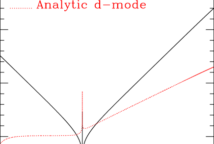
Figure 13: Evolutions of the isocurvature perturbation variable $S_{\phi\sigma}$ for our $d$-mode (solid line) and the analytic $d$-mode (dotted line). Panel (b) magnifies Panel (a) near the bounce. Panel (c) shows Panel (a) in logarithmic scale. The sharp divergences at the bounce occur because we have $\dot{\phi}=0$ at the bounce. For our $d$-mode $S_{\phi\sigma}$ nearly vanishes just before bounce near $\log{(a/a_{min})}\simeq 0.$; this is because we have found our $d$-mode initial condition beginning at this epoch, see the text for explanation. Figure 6 (c) shows that the adiabatic conditions for our $d$-modes of $\varphi_{v}$ are severely broken near the bounce. However, in Fig. 6 we argued that the $d$ mode of $\varphi_{v}$ is $(k/aH)^{2}$-order higher in the large-scale expansion compared with the $d$-mode of $\varphi_{\chi}$; i.e., the leading order $d$-mode of $\varphi_{v}$ has been canceled out, see Eqs. (39)-(42). Notice that in Fig. 6(d) the adiabatic condition for $d$-mode of $\varphi_{\chi}$ is well satisfied. Based on this observation, in Fig. 6 we have argued that despite the apparent severe breaking of the adiabatic condition for $\varphi_{v}$ the adiabatic nature of our $d$-mode initial condition is preserved throughout the bounce. In order to reinforce our such an argument in this figure we show the evolution of isocurvature perturbation variable $S_{\phi\sigma}$. The above figures show smooth behavior of our $d$-mode near the bounce. In case of the analytic $d$-mode, Figs. 11 (c) and (d) show that the adiabatic condition for $\varphi_{v}$ is severely broken near the bounce, and the adiabatic condition for $\varphi_{\chi}$ is sharply broken at the bounce and away from the bounce. As explained in Fig. 11, one sharp spike for $\varphi_{\chi}$ away from the bounce occurs because of the change of dominating mode between $d$ and $C$ mode, where the curvature variable $\varphi_{\chi}$ vanishes. However, in contrast with our $d$-mode, the above figure shows that for the analytic $d$-mode the isocurvature perturbation variable significantly changes its behavior at the bounce. Based on these behaviors we argue the following. Although the adiabatic condition for $\varphi_{v}$ of our $d$-mode initial condition is severely broken near the bounce, because the isocurvature perturbation shows the smooth behavior, the isocurvature perturbation does not give physical impact on the adiabatic nature of our $d$-mode throughout the bounce. Thus, although our $d$-mode initial condition shows apparently non-vanishing isocurvature mode (see Table 2), we argue that our $d$-mode initial condition keeps the adiabatic nature throughout the bounce. On the other hand, for the analytic $d$-mode both the adiabatic conditions are severely broken near the bounce and the isocurvature perturbation shows sharp change at the bounce. Thus, we argue that the isocurvature perturbation gives the physical impact on the adiabatic nature of the analytic $d$-mode; this analytic $d$-mode is based on an initial condition with ‘precise’ adiabatic condition (see Table 3). That is, for the analytic $d$-mode, although the initial condition is imposed assuming the adiabatic condition is exactly met, as the evolution proceeds the isocurvature perturbation is also excited, especially near the bounce. Thus, the numerical evolution shows that after the bounce the analytic initial $d$-mode in fact becomes a substantial mixture of the adiabatic and isocurvature modes.

IV.1.3 Method of finding our $C$- and $d$-modes

Here, we explain how we found ‘our $C$- and $d$-mode initial conditions’ which lead to correct behaviors of the $C$- and $d$-mode throughout the bounce. Since the $d$-mode is rapidly growing in a collapsing phase, thus dominating, we can easily find $d$-mode in that phase; similarly it is easy to find $C$-mode in an expanding phase. However, unless we impose a quite precise initial condition, it is very likely that, the relatively growing mode in that phase soon dominates the evolution. Thus, after the bounce a $d$-mode before the bounce is likely to switch to a dominating mode in an expanding phase which is the $C$-mode. We have shown that our $C$- and $d$-modes can be identified as the proper $C$- and $d$-mode which preserve their nature before and after the bounce. An imprecise initial condition, which tends to reproduce only the dominating solutions, can be regarded as a mixture of our (precise) $C$- and $d$-mode initial conditions. In Sec. IV.1.2, we showed that such a mixed initial condition leads to the break down of the adiabatic condition near the bounce and excitation of the iscurvature perturbation. Without a precise initial condition, it is hard to maintain $d$-mode nature after the bounce. Similarly, it is quite difficult to find $C$-mode initial condition which maintains its $C$-mode nature during the collapsing phase.

In order to find the precise initial condition for the $d$-mode we begin with the analytic initial condition imposed close to the bounce, and integrate forward and backward in time; the analytic initial condition is presented in Eq. (58) which is based on Eqs. (39) and (40). Our $d$-mode initial condition found in this way is presented in Table 2. As we have shown this $d$-mode initial condition leads to “the $d$-mode” which maintains its $d$-mode natures even after the bounce; see Fig. 6(a) and 6(b). Since the analytic initial condition in Eq. (58) assumes the exact adiabatic condition, the isocurvature perturbation of our $d$-mode naturally vanishes near the bounce, i.e., $S_{\phi\sigma}=0$; see Fig. 13.

Our $C$-mode initial condition is also found similarly. The $C$-mode behavior of $\varphi_{v}$ can be found if we begin with the analytic initial condition imposed close to the bounce, and integrate forward and backward in time. The behavior of $\varphi_{\chi}$ found in this way, however, shows $d$-mode behavior shortly before and shortly after the bounce. In order to find the $C$-mode behavior of $\varphi_{\chi}$ without appearance of the $d$-mode behavior near the bounce as in Fig. 4(b), we should begin with the analytic initial condition imposed away from bounce, and integrate forward and backward in time. In order to have the $C$-mode behavior in Fig. 4, we used the initial condition found by imposing the analytic initial condition at a point where $S_{\phi\sigma}$ vanishes (we call it an $S_{\phi\sigma}=0$ condition) in Fig. 12(c). In this way, behaviors of $C$-modes in Fig. 4, however, depend on whether we found our initial condition by imposing $S_{\phi\sigma}=0$ before or after the bounce as in Figs. 12(c) and 14(f). The $C$-mode behaviors in Figs. 4 and 7 are related to Fig. 12(c). In Fig. 14 we present the counterparts of Figs. 4 and 7 now related to Fig. 14(f). Comparison of these figures will show that near the bounce Fig. 14 is the reflection of Figs. 4 and 7 at the bounce. In Fig. 15 we present an additional case where we begin by imposing the analytic initial condition at one of the epochs of vanishing $\mu+p$. In this way, $\varphi_{\chi}=0$ at only one point, see Fig. 15(b) and 15(e). If we begin by imposing $S_{\phi\sigma}=0$ condition closer to or more away from the bounce we will have $d$-mode behavior of $\varphi_{\chi}$ near the bounce region. Thus, the $C$-mode behaviors in Figs. 4(b), 14(b), and 15(b) are closest to the analytic behavior of $C$-mode of $\varphi_{\chi}$ in Eq. (40).

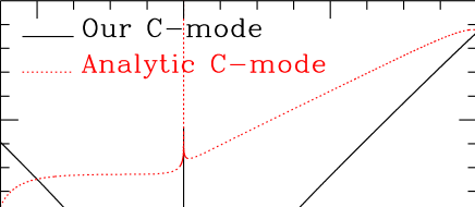
Figure 14: The same $C$-mode as in Figs. 4 and 7 now using slightly different way of finding our $C$-mode initial condition explained in the text. Panels (a)-(d) correspond to Figs. 4(a)-(d). Panel (e) corresponds to Fig. 7(f). Panel (f) corresponds to Fig. 12(c). Near the bounce these figures show reflection symmetry at the bounce compared with Figs. 4, 7(f), and 12(c). Figs. 7(a), 7(b), and 7(e) almost remain the same.

Figure 15: The same $C$-mode as in Figs. 4, 7(f), and 12(c) or Fig. 14, now for a particular way of finding our $C$-mode initial condition explained in the text. We imposed the analytic initial condition at one of the two $\mu+p=0$ epochs. Thus, Panels (a) and (c) have one less peak compared with Figs. 4(a) and (c); in Panel (a) we do not have a spike at the location of first arrow, whereas we do have such a spike in Fig. 4(a) though not visible. Evolution of $\varphi_{\chi}$ in Panel (b) shows only one vanishing point, see Panel (e). In Panel (d), the adiabatic condition of $\varphi_{\chi}$ also has one peak which is caused by vanishing $\varphi_{\chi}$. Panel (f) corresponds to Fig. 12(c), and shows slightly different location of minimum $S_{\phi\sigma}$.

IV.2 Tensor-type perturbations

The evolution of tensor-type perturbation is described by Eq. (64). Figures 16-18 show diverse behaviors of the tensor-type perturbation depending on initial conditions. Using the $\bar{C}_{\alpha\beta}$-mode initial condition in Eq. (65), Fig. 16 shows a conserved evolution of $C^{(t)}_{\alpha\beta}$ throughout the bounce: thus, we can clearly identify this as the $\bar{C}_{\alpha\beta}$-mode in Eq. (65). However, although we naively expected to be able to find a precise ${\bar{d}}_{\alpha\beta}$-mode initial condition in the collapsing phase which will be preserved as the same ${\bar{d}}_{\alpha\beta}$-mode even in the expanding phase, the numerical result in Fig. 17 shows that the ${\bar{d}}_{\alpha\beta}$-mode initial condition switches to the $\bar{C}_{\alpha\beta}$-mode.

This result differs from our following naive anticipation. The equation for tensor-type perturbation is quite similar to the one for $\varphi_{v}$ in an adiabatic limit: compare Eq. (64) with Eq. (30). In large-scale limits we have analytic solutions in Eqs. (65) and (39). In case of $d$-mode for the scalar-type perturbation in Fig. 6(a) we presented a proper $d$-mode evolution before and after the bounce. Thus, previously we anticipated that even for the tensor-type perturbation similarly we can find the proper initial condition which produces the ${\bar{d}}_{\alpha\beta}$-mode before the bounce continuing as the ${\bar{d}}_{\alpha\beta}$-mode after the bounce. In the following paragraph we can show that it is not possible to have such a behavior. Thus, any $\bar{d}_{\alpha\beta}$-mode initial condition in a collapsing phase is later dominated by an apparent $\bar{C}_{\alpha\beta}$-mode solution in an expanding era. This implies that we do not have the proper $\bar{d}_{\alpha\beta}$-mode which preserves its nature throughout the bounce. Figure 17(b) shows that the initially supplied $\bar{d}_{\alpha\beta}$-mode still survives as the same $\bar{d}_{\alpha\beta}$-mode even in the expanding era. Figure 17(a) shows that, after the bounce, $C^{(t)}_{\alpha\beta}$ is simply dominated by an additional $\bar{C}_{\alpha\beta}$-mode appearing after the bounce; this apparently comes from the lower-bound of integration of Eq. (65).

Here we can show why it is not possible to find the initial condition which remains as the $\bar{d}_{\alpha\beta}$-mode after the bounce. If the $\bar{d}_{\alpha\beta}$-mode in the collapsing phase could somehow switch to the same mode in the expanding phase, at the bounce $C^{(t)\prime}_{\alpha\beta}$ should either change its sign or cease to be differentiable. However, from Eq. (65), for $k=0$, we have

$$C^{{(t)}\prime}_{\alpha\beta}={\bar{d}_{\alpha\beta}(k)\over a^{2}},$$ (70)

where $\bar{d}_{\alpha\beta}$ is a temporal constant. Thus, once the sign of $\bar{d}_{\alpha\beta}$ is decided, then its sign is fixed throughout the evolution, and $C^{(t)\prime}_{\alpha\beta}$ is always differentiable. In case of the large-scale solution of $\varphi_{v}$ in Eq. (39), changing sign of $z^{2}$ plays an important role in explaining the different behaviors between $d$-mode of $\varphi_{v}$ and $\bar{d}_{\alpha\beta}$-mode of $C^{(t)}_{\alpha\beta}$; Fig. 8(d) shows that $\varphi_{v}$ does not only change its sign but also is not differentiable in a couple of places. For a non-vanishing $k$, from Eq. (66) we have

$$C^{{(t)}\prime}_{\alpha\beta}={\bar{d}_{\alpha\beta}\over a^{2}}-{k^{2}\over a^{2}}\left[\int^{\eta}{a^{2}}C^{(t)}_{\alpha\beta}(k,\eta)d\eta\right].$$ (71)

Since we are considering the ${\bar{d}}_{\alpha\beta}$-mode solution in the large-scale limit, the large-scale second-order correction term (the second term in RHS) in Eq. (71) should be negligible compared with the leading order term in Eq. (70); thus, the sign of $C^{{(t)}\prime}_{\alpha\beta}$ cannot be changed in that limit. This confirms that our numerical result for the ${\bar{d}}_{\alpha\beta}$-mode presented in Fig. 17(a) is unavoidable.

In Fig. 18, we present an evolution of initially near $\bar{C}_{\alpha\beta}$-mode which transits to the $\bar{d}_{\alpha\beta}$-mode after the bounce. Compared with the precise $\bar{C}_{\alpha\beta}$-mode in Fig. 16, in this Figure we introduced a small amount of initially negligible but non-vanishing $\bar{d}_{\alpha\beta}$-mode. The time derivative of $C^{(t)}_{\alpha\beta}$ in Fig. 18(b) shows that the apparent $\bar{d}_{\alpha\beta}$-mode in the expanding phase is exactly the one provided initially. After the bounce, the initially dominating $\bar{C}_{\alpha\beta}$-mode has been canceled out by a contribution from the lower-bound of integration of Eq. (65).

Table 4: The initial conditions for tensor-type perturbation with $k=0$. For $k=0$ the large-scale condition is met exactly. We take initial $\eta=-500$. Results based on these initial conditions are presented in Figs. 16-17.

variable	C-mode	d-mode
$C_{\alpha\beta}^{(t)}$	1.0E$-$05	1.0E$-$05
${C^{(t)}_{\alpha\beta}}^{\prime}$	0.	$-3./\eta\times C_{\alpha\beta}^{(t)}$

Figure 16: Evolution of $\bar{C}_{\alpha\beta}$-mode tensor-type perturbation. The behavior of $\bar{C}_{\alpha\beta}$-mode is similar to the C-mode of $\varphi_{v}$. The $\bar{C}_{\alpha\beta}$-mode nature of this mode is preserved throughout the bounce; i.e., the time derivative of $C^{(t)}_{\alpha\beta}$ vanishes throughout the evolution.

Figure 17: Panel (a) shows the behavior of initial $\bar{d}_{\alpha\beta}$-mode which apparently transits to the $\bar{C}_{\alpha\beta}$-mode after the bounce. It is not possible to find the initial condition which maintains the $\bar{d}_{\alpha\beta}$-mode behavior throughout the bounce: see the main text. Figure (b) presents the time derivative of $C^{(t)}_{\alpha\beta}$ which clearly shows that the initially provided $\bar{d}_{\alpha\beta}$-mode is present even after the bounce, this coincides with the analytic solution in Eq. (70). Meanwhile, Panel (a) shows that the initially introduced $\bar{d}_{\alpha\beta}$-mode is dominated by a newly generated $\bar{C}_{\alpha\beta}$-mode after the bounce. We take the initial condition in Table 4, thus $k=0$. Even in the case of nonvanishing $k$, the large-scale condition which compares $k^{2}$ with $a^{\prime\prime}/a$ term in Eq. (64) is well satisfied near the bounce.

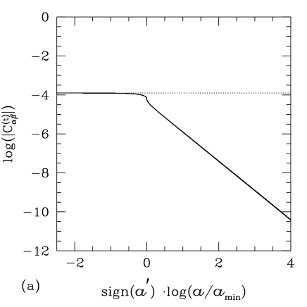
Figure 18: Panel (a) shows the behavior of initially near $\bar{C}_{\alpha\beta}$-mode which transits to the $\bar{d}_{\alpha\beta}$-mode after the bounce. As we are considering $k=0$ limit, the precise $\bar{C}_{\alpha\beta}$-mode in Fig. 16 sets $C^{(t)\prime}_{\alpha\beta}=0$. In this Figure we introduced a small negative value of $C^{(t)\prime}_{\alpha\beta}$= $-$1.9463109018142E-07$\times{C}^{(t)}_{\alpha\beta}$. This means that the present initial condition is a mixture of the dominating $\bar{C}_{\alpha\beta}$-mode plus a initially negligible but non-vanishing amount of the $\bar{d}_{\alpha\beta}$-mode. Panel (b) presents the time derivative of $C^{(t)}_{\alpha\beta}$ which shows that the apparent $\bar{d}_{\alpha\beta}$-mode in the expanding phase is actually the one provided initially.

V Power spectra

V.1 Scalar-type perturbations

As the origin of seed fluctuations for the large-scale structure we consider quantum fluctuations of the fields and the space-time metric ever present in the collapsing phase. Assuming certain dynamics of the scale factor we have the perturbation equations described by Bessel equations with the solutions in Hankel functions as in Eq. (49). The canonical quantization process well known in the literature leads to the same equations and solutions applicable to the quantum fluctuations. In order to correspond the large-scale solutions with the $C$- and $d$-mode decomposition in Eqs. (39) and (40) to the exact solutions with Hankel functions in Eq. (49), we follow hw2 . The power spectrum and spectral index are defined as

$$\mathcal{P}_{x}={k^{3}\over 2\pi^{2}}|x|^{2},\quad n_{S}-1\equiv{d\ln{\mathcal{P}_{x}}\over d\ln{k}},$$ (72)

where $x$ can be $\varphi_{v}(k,\eta)$ or $\varphi_{\chi}(k,\eta)$ in the Fourier space.

In the power-law case away from the bounce where the ghost field is negligible, Eqs. (30) and (31) lead to Bessel equations. Using the quantization based on the action formulation, we have the exact mode function solutions

$$\varphi_{v}(k,\eta)$$

$$\qquad=\left|{H\over\dot{\phi}}\right|{\sqrt{\pi|\eta|}\over 2a}[c_{1}(k)H_{\nu_{v}}^{(1)}(k|\eta|)+c_{2}(k)H_{\nu_{v}}^{(2)}(k|\eta|)],$$

$$\varphi_{\chi}(k,\eta)$$

$$\qquad={H\sqrt{\pi|\eta|}\over 2k\sqrt{2q}}[c_{1}(k)H_{\nu_{u}}^{(1)}(k|\eta|)+c_{2}(k)H_{\nu_{u}}^{(2)}(k|\eta|)],$$

$$\qquad\nu_{v}\equiv{3q-1\over 2(q-1)},\quad\nu_{u}\equiv{q+1\over 2(q-1)}.$$ (73)

The Hankel functions can be expanded as HM

$$H_{\nu}^{(1,2)}(k|\eta|) = \sum_{n=0}^{\infty}{1\over n!}\Bigg{[}-{(k|\eta|)^{2}\over 4}\Bigg{]}^{n}{1\over\sin\nu\pi}\times\Bigg{[}\Bigg{(}{k|\eta|\over 2}\Bigg{)}^{\nu}$$ (74)

$$\times{\pm ie^{\mp i\nu\pi}\over\Gamma(\nu+n+1)}+\Bigg{(}{k|\eta|\over 2}\Bigg{)}^{-\nu}$$

$$\times{\mp i\over\Gamma(-\nu+n+1)}\Bigg{]}.$$

In large scale limit, the first (second) term in the parenthesis dominates for $\nu<0$ $(\nu>0)$. In Eqs. (39) and (40) the leading orders of the $C$-modes are time independent whereas the leading orders of the $d$-modes behave as $\varphi_{v}\propto|\eta|^{2\nu_{v}}$ and $\varphi_{\chi}\propto|\eta|^{2\nu_{u}}$. Since

$$\varphi_{v}(k,\eta)\propto|\eta|^{\nu_{v}}H_{\nu_{v}}^{(1,2)}(k|\eta|),$$

$$\varphi_{\chi}(k,\eta)\propto k^{-1}|\eta|^{\nu_{u}}H_{\nu_{u}}^{(1,2)}(k|\eta|),$$ (75)

we can easily identify the first and the second terms in the parenthesis of Eq. (74) as the $d$-mode and the $C$-mode, respectively.

After taking the simple vacuum choice $c_{1}=1$ and $c_{2}=0$, the spectral indices for the $C$-mode and $d$-mode of $\varphi_{v}$ and $\varphi_{\chi}$ can be read as hw2

$$(n_{S}-1)_{\varphi_{v},C}=(n_{S}-1)_{\varphi_{\chi},C}={2\over 1-q},$$

$$(n_{S}-1)_{\varphi_{v},d}={4-6q\over 1-q},\quad(n_{S}-1)_{\varphi_{\chi},d}=-{2q\over 1-q}.$$

(76)

Notice that for the $C$-mode, the spectral index of $\varphi_{v}$ and $\varphi_{\chi}$ coincide.

The near Harrison-Zel’dovich scale-invariant spectrum corresponds to $n_{S}-1\simeq 0$ which is consistent with current observations of the cosmic microwave background radiation CMB and the large-scale structures LSS . The ekpyrotic or the cyclic scenario has $0<q\ll 1$, thus from Eq. (76) these scenarios have a scale-invariant spectrum for $d$-mode of $\varphi_{\chi}$, but these have a quite blue spectrum with $n_{S}-1\simeq 2$ for the $C$-mode hw2 ; incidentally, we have $n_{S}-1\simeq 4$ for the $d$-mode of $\varphi_{v}$. Although the $d$-mode of $\varphi_{\chi}$ shows a scale-invariant spectrum, we have shown that the $d$-mode eventually decays away in the expanding phase. Thus, we cannot see this spectrum in the current expanding phase of the universe. The observationally relevant one is the $C$-mode spectrum. Thus, for the ekpyrotic or the cyclic scenarios we have $n_{S}-1\simeq 2$ which is too blue compared with observations. Here, we assume a smooth nonsingular bounce with valid linear perturbation through the bounce; this differs from the original ekpyrotic/cyclic scenarios where the effective four dimensional spacetime goes through a singularity Ek . In the pre-Big Bang scenario we have $q=1/3$, thus $n_{S}-1=3$ for the $C$-mode pbb-pert .

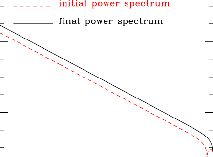
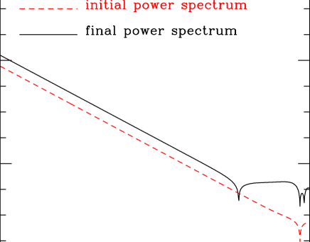
Figure 22: The same as Fig. 19, now for $d$-mode of $\varphi_{\chi}$. Panel (a) shows that the spectral index for our $d$-mode is $n_{S}-1=-4$ which agrees with our analytic result in Eq. (76). In case of analytic $d$-mode, only for large-scale ($\log{k}<-4$) perturbation the spectral index coincides with our $d$-mode case. In both Panels (a) and (c), due to time dependent evolution of $\varphi_{\chi}$, the amplitudes of power spectrum depend on our choice of initial and final epochs. Panels (b) and (d) show typical evolution of $\varphi_{v}$ corresponding to Panels (a) and (c), respectively, for two different wavenumbers. Panel (d) shows why the power spectrum at large wavenumber is enhanced compared with the one at small wavenumber.

In our simple bounce model case with $q={2/3}$, we have a scale-invariant spectrum for $d$-mode of $\varphi_{v}$, but the $d$-mode is meaningless because it decays away in an expanding phase. Our model shows a quite blue spectra for $C$-mode with $n_{S}-1=6$. In Figs. 19-22 we present the power spectra of $C$- and $d$-modes of $\varphi_{v}$ and $\varphi_{\chi}$ based on numerical integrations; we also present characteristic evolutions of $\varphi_{v}$ and $\varphi_{\chi}$. The initial spectra are based on the large-scale limit of Hankel function solutions in Eq. (73) which have their origins in quantum fluctuations in the collapsing phase. The spectral indices of final power spectra coincide with our analytic estimations made in Eq. (76). In Figs. 19-22 we present the initial and final power spectra from the analytic $C$- and $d$-modes together, and the characteristic evolutions of $\varphi_{v}$ and $\varphi_{\chi}$.

Based on numerical evolutions of certain initial conditions which are similar to the ‘analytic $C$- and $d$-modes’ of ours, the authors of AW reported that the $d$-mode in the collapsing phase survives as the $C$-mode in the expanding phase, see Fig. 11(a); similar results were also reported in Wands-1999 ; BF ; FB . This result leads these authors to claim that for $q=2/3$ the quantum fluctuations in the collapsing phase give rise to a scale-invariant spectrum in an expanding phase. Our numerical result in Fig. 21(c) apparently confirms this result. However, based on the behaviors of our $C$- and $d$-modes, the initial conditions used in these analytic $C$- and $d$-modes are mixture of the pure (our) $C$- and $d$-modes. Under these initial conditions, as the evolution proceeds we have shown that the isocurvature perturbation is also excited near the bounce, see Fig. 13. Thus, it is not correct to interpret that the final $C$-mode spectrum in the expanding phase is generated from the initial $d$-mode spectrum in the collapsing phase. In our interpretation, although the evolution begins with near $d$-mode (which is actually a mixture of our, thus precise, $C$- and $d$-modes), as we approach the bounce not only the $C$- and $d$-modes but also additional two isocurvature-type perturbations are all excited; this eventually leaves only the dominating mode (which is the $C$-mode in an expanding phase) after the bounce. In any case, our numerical result in Fig. 21(c) shows that near Harrison-Zel’dovich spectrum can be generated from the analytic $d$-mode initial condition with the help of the isocurvature perturbation simultaneously excited near the bounce. In case of our $C$- and $d$-modes where the $C$- and $d$-mode natures are preserved before and after the bounce, and the isocurvature perturbation is not excited. In that case, near Harrison-Zel’dovich spectrum in the $d$-mode of $\varphi_{v}$ is observationally not relevant.

A scale-invariant spectrum for the $C$-mode can be obtained for $q\gg 1$ which is the power-law inflation in an expanding phase. In the collapsing phase, however, $q>1$ implies that the relevant scales come inside the horizon near the bounce, thus invalidating the large-scale condition we used to get the above result. In the sub-horizon scale the modes oscillate, and lose their previous large-scale identity of the $C$- and the $d$-modes hw2 . From Eq. (76), for any model with $q<1$ during the quantum generation stage, we have $n_{S}-1>0$, thus having a blue spectrum.

Therefore, we conclude that while the large-scale condition is satisfied and the adiabatic condition is met (i.e., the isocurvature perturbation is not excited) during the bounce, it is not possible to obtain near Harrison-Zel’dovich scale-invariant density spectrum through a bouncing world model as long as the seed fluctuations were generated from quantum fluctuations of the curvature perturbation in the collapsing phase. This conclusion assumes that Einstein gravity is dominating throughout the bounce including the quantum generation stage.

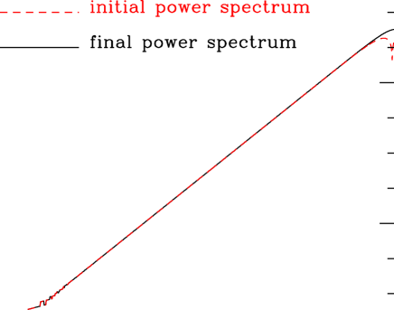
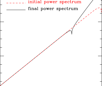
Figure 19: Power spectra and typical evolutions for the $C$-mode of $\varphi_{v}$. Panel (a) shows the initial and the final power spectra for our $C$-mode of $\varphi_{v}$. Panel (a) shows that the spectral index is $n_{S}-1=6$ which agrees with our analytic result in Eq. (76). Panel (c) shows the initial and the final power spectra for the analytic $C$-mode of $\varphi_{v}$. In this case, only for large-scale ($\log{k}<-4.5$) perturbation the spectral index coincides with our $C$-mode case. Panels (b) and (d) show typical evolutions of $\varphi_{v}$ corresponding to Panels (a) and (c), respectively, for two different wavenumbers. Panel (d) shows why the power spectrum at large wavenumber is enhanced compared with the one at small wavenumber. In Figs. 19-22 we take initial epoch at $\eta=-500$ [sign$(a^{\prime})\cdot$log$({a_{i}/a_{min}})\simeq-2.65$] and final epoch at $\eta=300$ [sign$(a^{\prime})\cdot$log$({a_{f}/a_{min}})\simeq 2.25$]. In order to get these power spectra, as the initial conditions both for our and analytic $C$- and $d$-modes, we use the Hankel function solutions in Eq. (73) in the large scale limit. In order to find our $C$- and $d$-mode initial conditions for different wavenumbers we use the same method explained in Sec. IV.1.3.

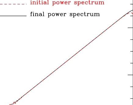
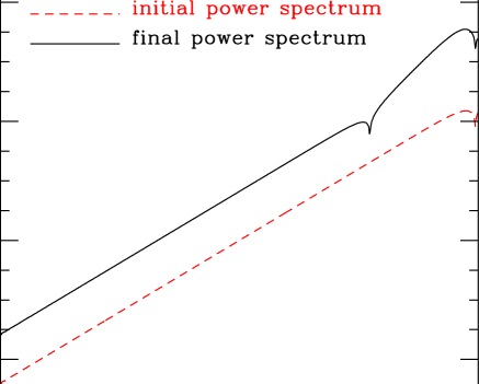
Figure 20: The same as Fig. 19, now for $C$-mode of $\varphi_{\chi}$. Panel (a) shows that the spectral index for our $C$-mode is also $n_{S}-1=6$ which agrees with our analytic result in Eq. (76). In case of analytic $C$-mode, only for large-scale ($\log{k}<-4$) perturbations the spectral index coincides with our $C$-mode case. In this case, however, due to time dependent evolution of $\varphi_{\chi}$, the amplitude of power spectrum simply depends on our choice of initial and final epochs. Panels (b) and (d) show typical evolution of $\varphi_{v}$ corresponding to Panels (a) and (c), respectively, for two different wavenumbers. Panel (d) shows why the power spectrum at large wavenumber is enhanced compared with the one at small wavenumber.

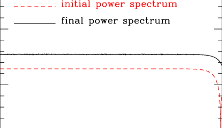
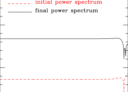
Figure 21: The same as Fig. 19, now for $d$-mode of $\varphi_{v}$. Panel (a) shows that the spectral index for our $d$-mode gives near Harrison-Zel’dovich scale-invariant spectrum ($n_{S}-1=0$) which agrees with our analytic result in Eq. (76). Panel (c) shows that the spectral index of the analytic $d$-mode also gives $n_{S}-1=0$. Panels (b) and (d) show typical evolution of $\varphi_{v}$ corresponding to Panels (a) and (c), respectively, for two different wavenumbers; these evolutions show why the final spectral indices resemble the initial ones. In both Panels (a) and (c), due to time dependent evolution of $\varphi_{\chi}$, the amplitudes of power spectrum depend on our choice of initial and final epochs. For $\log(k)>-2.5$ the scale comes inside the horizon when the final spectra are measured. Although the figure is not presented in AW , based on the power spectrum in Panel (c) the authors of AW reported that the bouncing world model can generate scale-invariant spectrum.

V.2 Tensor-type perturbations

The quantum fluctuations of the space-time metric detached from the fields provide seed fluctuations for the tensor-type perturbation (gravitational waves). For tensor-type perturbation, the power spectrum and spectral index are defined as

$$\mathcal{P}_{C_{\alpha\beta}^{(t)}}({\bf k},\eta)\equiv 2\sum_{l}{\mathcal{P}_{h_{l}}({\bf k},\eta)}\equiv 2\sum_{l}{k^{3}\over 2\pi^{2}}|h_{lk}|^{2},$$

$$n_{T}\equiv{d\ln{\mathcal{P}_{C^{(t)}_{\alpha\beta}}}\over d\ln{k}},$$ (77)

where we introduced a decomposition based on the two polarization states gw-quantum

$$C^{(t)}_{\alpha\beta}({\bf x},t) \equiv \sqrt{Vol}\int{d^{3}k\over(2\pi)^{3}}C^{(t)}_{\alpha\beta}({\bf x},t;{\bf k})$$

$$\equiv \sqrt{Vol}\int{d^{3}k\over(2\pi)^{3}}\sum_{l}e^{i{\bf k\cdot x}}h_{l{\bf k}}(t)e^{(l)}_{\alpha\beta}({\bf k}),$$

$$h_{l}({\bf x},t) \equiv {1\over 2}\sqrt{Vol}\int{d^{3}k\over(2\pi)^{3}}C^{(t)}_{\alpha\beta}({\bf x},t;{\bf k})e^{(l)\alpha\beta}({\bf k})$$ (78)

$$= \sqrt{Vol}\int{d^{3}k\over(2\pi)^{3}}e^{ik\cdot x}h_{lk}(t),$$

with $l=+,\times$; the polarization tensors $e^{(+)}_{\alpha\beta}$ and $e^{(\times)}_{\alpha\beta}$ indicate the plus (+) and cross ($\times$) polarization states with $e^{(l)}_{\alpha\beta}({\bf k})e^{(l^{\prime})\alpha\beta}({\bf k})=2\delta_{ll^{\prime}}$.

In order to correspond our large-scale solution in Eq. (65) to the exact solution in Eq. (68), we follow a similar reasoning used for the $\varphi_{v}$. In Eq. (65) the leading order of the $\bar{C}_{\alpha\beta}$-mode is time independent whereas the leading order of $\bar{d}_{\alpha\beta}$-mode behaves as $C_{\alpha\beta}^{(t)}\propto|\eta|^{-2\nu_{g}}$. Since

$$C_{\alpha\beta}^{(t)}(k,\eta)\propto|\eta|^{-\nu_{g}}H_{\nu_{g}}^{(1,2)}(k|\eta|),$$ (79)

we can easily identify the first term in the parenthesis of Eq. (74) as the $\bar{C}_{\alpha\beta}$-mode and second term as the $\bar{d}_{\alpha\beta}$-mode. We can read the spectral indices for $\bar{C}_{\alpha\beta}$ and $\bar{d}_{\alpha\beta}$ as

$$n_{T,\bar{C}_{\alpha\beta}}={2\over 1-q},\quad n_{T,\bar{d}_{\alpha\beta}}={4-6q\over 1-q}.$$ (80)

These spectral indices of tensor-type perturbation coincide with the spectral indices of the $\varphi_{v}$ in Eq. (76).

From the classical evolution of the tensor-type perturbation studied in Sec. IV.2 we notice that both the initial $\bar{C}_{\alpha\beta}$- and $\bar{d}_{\alpha\beta}$-modes survive as the $\bar{C}_{\alpha\beta}$-mode after the bounce. If both modes are generated from the quantum fluctuations with comparable amplitude, as the collapsing phase proceeds the initial $\bar{C}_{\alpha\beta}$-mode becomes negligible compared with the initial $\bar{d}_{\alpha\beta}$-mode. Thus, after the bounce the dominant $\bar{C}_{\alpha\beta}$-mode should have origin from the initial $\bar{d}_{\alpha\beta}$-mode; as the $\bar{d}_{\alpha\beta}$-mode grows rapidly in the collapsing phase, its final amplitude surely depends on the duration of the collapse after its quantum origin. This is in contrast to the situation of the scalar-type perturbation where the initial $d$-mode remains as the $d$-mode even after the bounce, thus decays away in the expanding phase.

In the pre-big bang scenario with $q=1/3$, we have $n_{T,{\bar{C}_{\alpha\beta}}}=3$ and $n_{T,{\bar{d}_{\alpha\beta}}}=3$. In the ekpyrotic or cyclic models with $q\simeq 0$, we have $n_{T,{\bar{C}_{\alpha\beta}}}=2$ and $n_{T,{\bar{d}_{\alpha\beta}}}=4$. Notice that it is the $\bar{d}_{\alpha\beta}$-mode initial condition in the collapsing phase which survives as the dominating $\bar{C}_{\alpha\beta}$-mode after the bounce in case of the tensor-type perturbation. Thus, the dominating $\bar{C}_{\alpha\beta}$-mode perturbation in expanding phase produced in the ekpyrotic and cyclic scenarios has $n_{T}=4$ spectrum; this also differs from $n_{T}=2$ which is claimed by the authors of these scenarios Ek . Meanwhile, in our simple bounce model with $q=2/3$, we have $n_{T,{\bar{C}_{\alpha\beta}}}=6$ and $n_{T,{\bar{d}_{\alpha\beta}}}=0$. From Eq. (80) we notice that only for $q=2/3$, thus $w=0$, we have a scale-invariant near Harrison-Zel’dovich type spectrum $n_{T,{\bar{d}_{\alpha\beta}}}=0$ for the tensor-type perturbation. In Fig. 23 we present the final spectra of the initial $\bar{C}_{\alpha\beta}$- and $\bar{d}_{\alpha\beta}$-modes in case of $w=0$; these numerical results coincide with our analytic estimation made above.

Figure 23: This figure shows the final power spectra for initial ${\bar{C}}_{\alpha\beta}$- and ${\bar{d}}_{\alpha\beta}$-modes. The initial ${\bar{d}}_{\alpha\beta}$-mode has a scale-invariant spectrum with $n_{T,\bar{d}_{\alpha\beta}}=0$, and ${\bar{C}}_{\alpha\beta}$-mode has very blue spectrum with $n_{T,\bar{C}_{\alpha\beta}}=6$; these agree with our analytic result in Eq. (80). The amplitudes of power spectra depend on background properties. For $\log(k)>-2$ the scale comes inside the horizon when the final spectra are measured.

VI Discussion

In order to explain the origin of large-scale structure in the universe, several models of bouncing scenarios pbb ; Ek were suggested as possible alternatives to the inflation. The pre-big bang scenario in pbb failed to produce the observationally required scale-invariant spectrum for scalar-type perturbation; this model has $q=1/3$ thus leads to $(n_{S}-1)_{\varphi_{v},C}\simeq 3$ and $n_{T,\bar{d}_{\alpha\beta}}\simeq 3$. Whereas, the authors of ekpyrotic or cyclic scenarios Ek claimed that their scenarios successfully produce the required spectrum. The latter authors find that the quantum fluctuations of $d$-mode of $\varphi_{\chi}$ show near Harrison-Zel’dovich scale-invariant spectrum and claimed that this mode gives rise to the $C$-mode after the bounce. As long as the adiabatic condition and the large-scale condition are met during the bounce (and, of course, assuming the linear perturbation theory survives the bounce) from the analytic point of view we can see that $d$-mode before the bounce remains as the same $d$-mode after the bounce and similarly for the $C$-mode. Since the $d$-mode is transient in an expanding phase, we have to consider the $C$-mode as the proper seed for the large-scale structure. For the ekpyrotic or cyclic scenarios with $0<q\ll 1$ the quantum fluctuations of the $C$-mode of both $\varphi_{\chi}$ and $\varphi_{v}$ show very blue spectra with $n_{S}-1\simeq 2$, thus fail to explain the observation.

In this work we have confirmed the above expectation based on analytic arguments made in HN-bounce by following the $C$- and $d$-modes numerically in a simple nonsingular bouncing world model. We found the $C$- and $d$-mode initial conditions in which the nature of the $C$- and $d$-modes are preserved through our nonsingular bounce world model. Thus, we have shown that the scale-invariant spectrum claimed by the proponents of ekpyrotic or cyclic models is not possible if the bounce occurs non-singularly as in our toy bounce model. In the original ekpyrotic/cyclic scenarios based on five dimension the effective four dimensional spacetime goes through a singularity Ek , and the situation cannot be handled using perturbation theory in Einstein gravity. Our results also imply that it is not possible to generate near Harrison-Zel’dovich scale-invariant spectrum from the quantum fluctuations in the collapsing phase as long as the isocurvature perturbation is not excited significantly near the bounce. We state again the assumptions we made to get such a conclusion: (i) Einstein’s gravity and linear perturbation theory work throughout the evolution, (ii) quantum fluctuations of a minimally coupled scalar field in a collapsing phase provide seed curvature (adiabatic) mode fluctuations for the large-scale structure, (iii) the large-scale conditions are met during the bounce, (iv) the adiabatic conditions are met during the bounce. We have carefully examined that the latter two conditions are often violated subtly near the bounce without affecting curvature perturbation natures in the large-scale limit.

In our simple bounce model we introduced a ghost field $\sigma$ only to have a natural bounce in the background. The presence of additional ghost field in addition to the ordinary minimally coupled scalar field $\phi$ (which is introduced to have curvature-type seed fluctuations), however, forces us to handle a fourth-order differential equation for the scalar-type perturbation. In order to have a nonsingular bounce we need $\sigma$ to be important only near the bounce. However, the presence of ghost field could potentially generates the isocurvature-type perturbation $S_{\phi\sigma}$ due to the perturbed ghost field near the bounce. Our above conclusion forbidding near Harrison-Zel’dovich spectrum from the bouncing model is based on assuming no isocurvature perturbation being excited near the bounce (i.e., the adiabatic conditions are well met during the bounce). Under this condition we have found the $C$- and $d$-modes which preserve their nature before and after the bounce.

By using the analytic $C$- and $d$-mode initial conditions we have shown that it is actually possible to have near Harrison-Zel’dovich spectrum from the analytic $d$-mode initial condition of $\varphi_{v}$ for $q=2/3$, see Figs. 21(c) and 21(d); this result was reported in AW ; Wands-1999 ; BF ; FB . In this case, although Fig. 21(d) shows that the initial $d$-mode before the bounce is switched into an apparently $C$-mode after the bounce, such a transition occurs because isocurvature perturbation is significantly excited near the bounce; i.e., under such an initial condition all four modes (two $C$- and $d$- curvature modes and two isocurvature modes) are excited near the bounce, thus mixing modes before and after the bounce. Our numerical results show that, unless we impose a rather precise initial conditions, it is very likely that we can easily have only relatively dominating mode during the evolution: these are the $d$-mode in a collapsing phase, and the $C$-mode in an expanding phase. Figures 10(a), 10(b), 11(a), and 11(b) based on the analytic $C$- and $d$-modes clearly show such mixed behaviors between the $C$- and $d$-modes. We have shown that these are because the analytic $C$- and $d$-mode initial conditions can be viewed as mixtures of our (precise) $C$- and $d$-modes, i.e., imprecise. In addition, even the isocurvature perturbation caused by the presence of the ghost field is excited near the bounce.

We have shown that for the tensor-type perturbation, however, it is the $\bar{d}_{\alpha\beta}$-mode initial condition which survives as the dominating $\bar{C}_{\alpha\beta}$-mode in the expanding phase. Thus, for the ekpyrotic or cyclic scenarios with $0<q\ll 1$, we have $n_{T,\bar{d}_{\alpha\beta}}\simeq 4$; this also differs from the predictions made by the original authors of these scenarios who claimed $n_{T,\bar{C}_{\alpha\beta}}\simeq 2$ as the dominating mode.

In conclusion, as long as the large-scale condition and the adiabatic condition are satisfied, we numerically show that the $C$-mode in a collapsing phase leads to the observationally relevant quantity in the expanding phase. The $d$-mode, in contrast, remains as the same $d$-mode even after the bounce. Thus, under these conditions, it is not possible to obtain a scale-invariant spectrum in the bounce cosmological model based on the quantum fluctuations in the collapsing phase. Equation (76) shows that only for $q\gg 1$ during quantum generation stage the bounce model can produce near Harrison-Zel’dovich scale-invariant density spectrum. However, since this leads to a violation of the large-scale condition near the bounce we cannot use this result; the modes are mixed up and begin to oscillate, thus we cannot trace the $C$- and $d$-mode nature through the bounce. That is, as the scales come inside the horizon, perturbations start oscillations and lose their large-scale memory of the original $C$- and $d$-modes. For the tensor-type perturbation, it is the initial $\bar{d}_{\alpha\beta}$-mode which survives as the dominating $\bar{C}_{\alpha\beta}$-mode in the expanding phase.

We may summarize the final spectral indices for the scalar- and tensor-type perturbations as

$$(n_{s}-1)_{C}={2\over 1-q},\quad n_{T,{\bar{d}_{\alpha\beta}}}={4-6q\over 1-q},$$ (81)

where we have $a\propto|t|^{q}$ during the quantum generation stage before bounce. Meanwhile, if the initial seed fluctuations were generated from quantum fluctuations during expanding phase (without or after bounce), the observationally relevant perturbations have

$$(n_{s}-1)_{C}={2\over 1-q}=n_{T,{\bar{C}_{\alpha\beta}}},$$ (82)

which is the well known result in the literature Stewart-Lyth-1993 ; hw1 . Notice the difference in the gravitational wave power spectrum generated between the bounce and the inflation scenarios.

Our analysis in this work is based on a specific nonsingular bounce model with two scalar fields. Using this specific model we were able to follow numerically the evolutions of scalar- and tensor-type perturbations through the bounce. We have shown that the nature of large-scale decomposition of the adiabatic solutions far away from the bounce, i.e., the $C$- and $d$-modes, is preserved throughout the bounce as long as the two conditions (the large-scale and adiabatic ones) are met. Throughout the bounce we have numerically monitored that these conditions are physically met as long as we take the correct and precise initial conditions which assure the $C$- and $d$-mode natures; we also have monitored the evolution of isocurvature perturbation. In order to help readers to reproduce our numerical results, in Table 2 we have provided the precise initial conditions we used. Because the above argument was originally based on the analytic solutions with general equation of state or field potential, our numerical analysis based on specific bounce model may have more generic implications which go beyond the specific model we used. Our concrete numerical study assures that our previous conclusions based on analytic reasons in hw1 ; hw2 ; HN-bounce are valid.

In this work, we have assumed Einstein’s gravity and spatially homogeneous-isotropic background world model with linear perturbations are valid throughout the bounce. In realistic situation, however, it is likely that in the collapsing phase as the model approaches the bounce the perturbations of all three types grow rapidly and eventually become nonlinear, thus invalidating the spatially homogeneous-isotropic Friedmann background world model. Furthermore, as the scale factor shrinks we reach the high energy scale where quantum corrections of Einstein’s gravity likely lead to serious correction terms in the gravity itself. Although we have used a ghost field as the bounce agent in Einstein’s gravity, it is also likely that the quantum correction terms can cause nonsingular bounce more naturally bounce-pert-others . In this work we have assumed that the linear perturbation theory survives throughout the bounce which certainly restricts the allowed bounce model.

Acknowledgments

We thank Drs. Hyerim Noh and Ewan Stewart for useful discussions. This work was supported by the Korea Research Foundation Grant No. 2003-015-C00253 and KNURT (Kyungpook National University Research Team) Fund 2002.

References

- (1) E.R. Harrison, Phys. Rev. D 1, 2726 (1970); Ya.B. Zel’dovich, Mon. Not. R. Astr. Soc. 160, 1 (1972).
- (2) M. Gasperini and G. Veneziano, Astropart. Phys. 1, 317 (1993).
- (3) R. Brustein, M. Gasperini, M. Giovannini, V. F. Mukhanov and G. Veneziano, Phys. Rev. D 51, 6744 (1995); J. Hwang, Astropart. Phys. 8, 201 (1998).
- (4) J. Khoury, B.A. Ovrut, P.J. Steinhardt and N. Turok, Phys. Rev. D 64, 123522 (2001); 66, 046005 (2002); P.J. Steinhardt, N. Turok, Science 296, 1436 (2002).
- (5) D.H. Lyth, Phys. Lett B 524 1 (2002); 526, 173 (2002)
- (6) R. Brandenberger, F. Finelli, JHEP 0111, 056 (2001)
- (7) J. Hwang, Phys. Rev. D 65 063514 (2002).
- (8) J. Hwang, H. Noh, Phys. Lett. B 545, 207 (2002).
- (9) J. Hwang, H. Noh, Phys. Rev. D 65 124010 (2002).
- (10) J.M. Bardeen, Phys. Rev. D 22, 1882 (1980).
- (11) A.A. Starobinsky, Sov. Phys. JETP Lett. 30, 682 (1979); C. Cartier, E.J. Copeland, M. Gasperini, Nucl. Phys. B 607, 406 (2001); R.H. Brandenberger, S.E. Joras, J. Martin, Phys. Rev. D 66, 083514 (2002); R. Durrer, F. Vernizzi, Phys. Rev. D 66, 083503 (2002); J. Martin, P. Peter, N. Pinto-Neto, D.J. Schwarz, Phys. Rev. D 65, 123513 (2002); P. Peter, N. Pinto-Neto, Phys. Rev. D 66, 063509 (2002); S. Tsujikawa, Phys. Lett. B 526, 179 (2002); S. Tsujikawa, R. Brandenberger, F. Finelli, Phys. Rev. D 66, 083513 (2002); M. Gasperini, M. Giovannini, G. Veneziano, Phys. Lett. B 569, 113 (2003); C. Gordon, N. Turok, Phys. Rev. D 67, 123508 (2003); F. Finelli, JCAP 0310, 011 (2003); F. Finelli, Phys. Lett. B 575, 165 (2003); J. Martin, P. Peter, Phys. Rev. D 68, 103517 (2003); J. Martin, P. Peter, N. Pinto-Neto, D. J. Schwarz, Phys. Rev. D 67 028301 (2003); P. Peter, N. Pinto-Neto, D.A. Gonzalez, JCAP 0312, 003 (2003); M. Gasperini, M. Giovannini, G. Veneziano, Nucl. Phys. B 694, 206 (2004); N. Deruelle, A. Streich, Phys. Rev. D 70, 103504 (2004); P. Creminelli, A. Nicolis, M. Zaldarriaga, Phys. Rev. D71, 063505 (2005); V. Bozza, G. Veneziano, Phys. Lett. B625, 177 (2005); V. Bozza, G. Veneziano, JCAP 0509, 007 (2005); T.J. Battefeld, G. Geshnizjani, Phys. Rev. D 73, 048501 (2006); T.J. Battefeld, G. Geshnizjani, Phys. Rev. D 73, 064013 (2006); V. Bozza, JCAP 0602, 009 (2006).
- (12) L.E. Allen, D. Wands, Phys. Rev. D 70, 063515 (2004).
- (13) F. Finelli, R. Brandenberger, Phys. Rev. D 65, 103522 (2002).
- (14) D. Wands, Phys. Rev. D 60, 023507 (1999).
- (15) R.V. Buniy, S.D.H. Hsu, Phys. Lett. B 632, 543 (2006).
- (16) F. Lucchin, S. Matarrese, Phys. Rev. D 32, 1316 (1985).
- (17) J.M. Bardeen, Cosmology and Particle physics, edited by L Fang and A Zee (London:Gordon and Breach) (1988).
- (18) J. Hwang, Astrophys. J. 375 443 (1991).
- (19) J. Hwang, H. Noh, Phys. Rev. D 71, 063536 (2005).
- (20) J. Hwang, H. Noh, Class. Quant. Grav. 19, 527 (2002).
- (21) E.M. Lifshitz, J. Phys. (USSR) 10, 116 (1946); L.P. Grishchuk, Sov. Phys.JETP 40, 409 (1975).
- (22) M. Abramowitz, I. A. Stegun (Eds.), Handbook of Mathematical Functions, Dover, New York, 1972.
- (23) G.F. Smoot, et al., Astrophys. J. 396, L1 (1992); D.N. Spergel, et al., Astrophys. J. Suppl 148, 175 (2003); M. Tegmrk, et al., Phys. Rev. D 69, 103501 (2004).
- (24) M. Colless, et al., 2003, Preprint astro-ph/0306581; K. Abazajian, et al. in http://www.sdss.org/dr3/ (2004).
- (25) L.H. Ford, L. Parker, Phys. Rev. D 16, 1601 (1977); L. F. Abbott, M. B. Wise, Nucl. Phys. B 264, 541 (1984); A. A. Starobinsky, Sov. Astron. Lett 11, 133 (1985); B. Allen, S. Koranda, Phys. Rev. D 50, 3713 (1994). J. Hwang, Class. Quant. Grav. 15, 1401 (1998).
- (26) E.D. Stewart, D.H. Lyth, Phys. Lett. B 302, 171 (1993).