The DEEP2 Galaxy Redshift Survey: Clustering of Quasars and Galaxies at $z=1$

Abstract

We present the clustering of DEEP2 galaxies at $0.7<z<1.4$ around quasars identified using both the SDSS and DEEP2 surveys. We measure the two-point cross-correlation of a sample of 36 optically-selected, spectroscopically-identified quasars from the SDSS and 16 more found in the DEEP2 survey with the full DEEP2 galaxy sample over scales $0.1<r_{p}<10$ $h^{-1}$ Mpc. The clustering amplitude is found to be similar to the auto-correlation function of DEEP2 galaxies, with a relative bias of $b=0.89\pm 0.24$ between quasars and DEEP2 galaxies at $z\sim 1$. No significant dependence is found on scale, quasar luminosity, or redshift over the ranges we probe here. The clustering amplitude errors are comparable to those from significantly larger quasar samples, such as the 2dF QSO Redshift Survey. This results from the statistical power of cross-correlation techniques, which exploit the fact that galaxies are much more numerous than quasars. We also measure the local environments of quasars using the $3^{\rm rd}$-nearest-neighbor surface density of surrounding DEEP2 galaxies. Quasars are found in regions of similar mean overdensity as blue DEEP2 galaxies; they differ in environment from the red DEEP2 galaxy population at $2\sigma$ significance. Our results imply that quasars do not reside in particularly massive dark matter halos at these redshifts, with a mean dark matter halo mass of $M_{200}\sim 3\times 10^{12}M_{\sun}$ in a concordance $\Lambda$CDM cosmology.

1. Introduction

There is growing evidence that most galaxies have a supermassive black hole in their nucleus (for a review, see e.g. Richstone et al. 1998). Accretion onto these supermassive black holes likely powers quasars, which now appear to be highly relevant for galaxy formation and evolution models. In particular, the observed correlation between black hole mass and the velocity dispersion of stars in the bulge components of galaxies (Gebhardt et al. 2000; Ferrarese & Merritt 2000) indicates some form of feedback or connection between the growth of black holes and their parent galaxies. In addition, quasar or active galactic nuclei (AGN) feedback may play a significant role in reproducing the observed color-magnitude diagram at high redshift (Springel, Di Matteo, & Hernquist 2005; Croton et al. 2006).

It remains unclear what physical mechanism fuels quasars and what impact their presence has on galaxy formation and evolution. Quasar clustering measurements can be used to infer their lifetimes and large-scale environments, which help address these issues. Clustering measurements lead to an estimate of the mean dark matter halo mass of a given population, by using semi-analytic methods or cosmological dark matter N-body simulations to relate the observed number density and clustering strength of a data sample to its parent dark matter halo population (e.g., Kaiser 1984; Efstathiou et al. 1988; Cole & Kaiser 1989; Mo & White 1996; Sheth & Tormen 1999). This allows the population to be placed in a cosmological context, useful for comparisons with simulations and galaxy evolution models. Quasar clustering analyses can further constrain the physics behind the creation and fueling of quasars from the lifetimes inferred by the ratio of the quasar number densities to those of their parent dark matter halos (Haiman & Hui 2001; Martini & Weinberg 2001; Wyithe & Loeb 2005).

The advent of the 2dF QSO Redshift Survey (Croom et al. 2004b) allowed the first robust measurements of the quasar clustering amplitude using a large sample covering sizeable areas of the sky, $\sim 20,000$ objects in $\sim 700$ square degrees (Croom et al. 2002; Porciani, Magliocchetti, & Norberg 2004; Croom et al. 2005). Their main results are: 1) quasars between redshift $0.3<z<2.2$ show similar clustering as local galaxies, well-fit by a power-law with a clustering scale-length of $r_{0}=4.8\ (+0.9/-1.5)$ $h^{-1}$ Mpc and a slope of $\gamma=1.5\pm 0.2$; 2) the clustering amplitude shows little dependence on quasar luminosity (within the large error bars); and 3) that amplitude increases with redshift from $0.5<\bar{z}<2.5$. Myers et al. (2006) confirm these conclusions using the projected angular clustering of $\sim$80,000 quasars in the Sloan Digital Sky Survey (SDSS). These results generally support a picture in which quasar luminosity is not strongly correlated with the parent dark matter halo mass, and characteristic quasar host halo masses are $\sim 10^{12}-10^{13}M_{\sun}$ at $z\sim 1-2$. Additionally, only a few percent of the potential parent halos actually host a quasar (Porciani, Magliocchetti, & Norberg 2004), and the inferred quasar lifetime is not long, $\sim 10^{7}$ years.

Unfortunately, the error bars on the clustering amplitudes estimated from the quasar auto-correlation function are still large, due to their relatively low number density. Studying the clustering of galaxies around quasars (by measuring the cross-correlation function of quasars and galaxies) can afford more precise measurements of the clustering amplitude of quasars, as the number density of galaxies is much higher (e.g., Kauffmann & Haehnelt 2002). It also provides a measure of the local environment in which quasars reside, which is relevant to understanding the physics of quasar fueling.

It has long been known that quasars are associated with enhancements in the distribution of galaxies (Bahcall, Schmidt, & Gunn 1969; Seldner & Peebles 1979; Yee & Green 1984, 1987; Bahcall & Chokshi 1991; Laurikainen & Salo 1995; Smith, Boyle, & Maddox 1995; Hall & Green 1998; Smith, Boyle, & Maddox 2000). However, there has been significant scatter in these measurements of quasar-galaxy correlations (see Brown, Boyle, & Webster 2001, Table 1 for a compilation of recent studies) caused by heterogeneous quasar samples, methodology, and imaging depths. Large surveys such as the 2dF and SDSS provide homogeneous samples of $\sim 10,000$ quasars/AGN surrounded by $\sim 100,000$ galaxies, providing an opportunity to robustly study the clustering of galaxies around low redshift quasars.

For quasars at $z<0.3$, Croom et al. (2004a) show that the quasar-galaxy cross-correlation function in 2dF data is the same as the galaxy auto-correlation function, measured in redshift space on scales of $s=1-20$ $h^{-1}$ Mpc. Wake et al. (2004) measure the clustering amplitude of AGN in redshift space for $z<0.2$ in the SDSS DR1 data, where AGN are selected using classic emission-line ratio diagnostics and they have excluded broad-line quasars. They find that AGN have a similar clustering strength as galaxies in the same redshift range, with a small anti-bias with respect to the full SDSS galaxy sample of $b=0.92\pm 0.03$ on scales $s\sim 0.4-20$ $h^{-1}$ Mpc. Comparing their results to dark matter simulations, they conclude that the minimum host dark matter halo mass for these AGN is $M_{min}=2\times 10^{12}M_{\sun}$. Constantin & Vogeley (2006) compare the redshift-space auto-correlation function of narrow-line AGN in SDSS data and find that Seyferts are less clustered than the full galaxy sample, while LINERS show similar clustering properties to all galaxies. (Serber et al. 2006) study the environments of $z<0.4$ luminous ($M_{i}<-22$) quasars in the SDSS and find that quasars cluster similarly to $L^{*}$ galaxies on scales $\sim 1$ $h^{-1}$ Mpc, in agreement with the aforementioned studies. However, on smaller scales at $r<100$ $h^{-1}$ kpc they find that quasars reside in regions overdense by a factor of $1.4-3$ compared to regions around $L^{*}$ galaxies, with the larger density enhancement occurring for the most luminous quasars ($M_{i}<-23.3$) in their sample.

At higher redshifts Adelberger & Steidel (2005) measure the cross-correlation of 79 AGN and $\sim$1600 Lyman-break galaxies at $2<z<3$. They find that the cross-correlation scale-length is $r_{0}\sim 5\pm 2$ $h^{-1}$ Mpc, similar to the clustering amplitude of Lyman-break galaxies themselves, and does not depend on AGN luminosity, from which they infer that brighter and fainter AGN reside in dark matter halos of similar mass and therefore fainter AGN are longer lived.

In this paper we present the first measurements of the quasar-galaxy cross-correlation function at $z\sim 1$, using data from the SDSS and DEEP2 galaxy redshift surveys. Because the selection function of DEEP2 galaxies has been precisely quantified, we are able to robustly correct for small-scale selection biases in the galaxy sample allowing us to measure the clustering strength as a function of scale from $0.1<r<10$ $h^{-1}$ Mpc. We also present measurements of the mean local environment of quasars at $z\sim 1$, compared to galaxies in the DEEP2 survey. The layout of the paper is as follows: §2 presents the quasar and galaxy data samples; §3 discusses the methods used to estimate the cross-correlation function; clustering and environment results are presented in §4 and §5 and discussed in §6.

2. SDSS Quasar and DEEP2 Galaxy Samples

We use data from both the SDSS and DEEP2 redshift surveys where they overlap – ie., in the DEEP2 fields – in the redshift range $0.7<z<1.4$. There are 36 spectroscopically-identified quasars from the SDSS and an additional 16 quasars in the DEEP2 Galaxy Redshift Survey in the volume sampled by DEEP2 galaxies. We measure cross-correlation statistics for three quasar/AGN samples: 1) all SDSS quasars, 2) all SDSS and DEEP2 quasars brighter than $M_{B}<-22$, and 3) all SDSS and DEEP2 quasars and an additional 7 DEEP2 type 1 AGN (labeled as the ’all quasars’ sample).

Redshifts and $M_{B}$ magnitudes for quasars in both the SDSS and DEEP2 samples are shown in Fig. 1, and details of each sample are given below. The median redshifts of the SDSS quasar sample, the DEEP2 quasar and AGN sample, and the full combined sample are $z_{median}=1.01$, 0.80, and 0.99, respectively. The redshifts of the quasars used in this study were computed via cross-correlation with a composite quasar template. For the SDSS quasars, the spectral coverage is 3800-10000 Å; in the redshift range $z=0.7-1.4$ the MgII 2798 Å and [OIII] 5007 Å emission lines dominate measurements of the quasar redshift. For the DEEP2 observations, the smaller spectral coverage of $\sim$6200-9400 Å results in either MgII or [OIII] being present. Boroson (2005) find that the [OIII] emission line has an average shift of 40 km s^-1 and a dispersion of $<$100 km s^-1 about the systemic reference frame defined by low-ionization forbidden lines. Richards et al. (2002a) find that the MgII emission line has a median shift of 97 km s^-1 and a dispersion of 269 km s^-1 about [OIII] (assumed to be systemic). Thus a very conservative estimate of the errors in the quasar redshifts due to both shifts from systemic and errors in the redshift determination would be $<$ 500 km s^-1, or $dz<0.003$, which corresponds to 5 $h^{-1}$ Mpc at $z=1.0$.

2.1. The SDSS Quasar Sample

The SDSS uses a dedicated 2.5m telescope and a large format CCD camera (Gunn et al. 1998, 2006) at the Apache Point Observatory in New Mexico to obtain images in five broad bands ($u$, $g$, $r$, $i$ and $z$, centered at 3551, 4686, 6166, 7480 and 8932 Å, respectively; Fukugita et al. 1996; Stoughton et al. 2002) of the high Galactic latitude sky in the Northern Galactic Cap. Based on these imaging data, spectroscopic targets chosen by various selection algorithms are observed with two double spectrographs producing spectra covering 3800–9200 Å with a spectral resolution ranging from 1800 to 2100. Details of the spectroscopic observations can be found in York et al. (2000), Castander et al. (2001), and Stoughton et al. (2002). Additional details on the SDSS data products can be found in Abazajian et al. (2003, 2004, 2005).

We briefly summarize the essential details about the SDSS quasar catalog, and refer the reader to (Schneider et al. 2005) for a more thorough discussion. In the redshift range of interest to us here $0.7<z<1.4$, the primary SDSS low redshift target selection algorithm Richards et al. (2002b) imposes an $i$ magnitude limit of 19.1, and the SDSS quasar catalog has very high completeness Vanden Berk et al. (2005) above this limit. Supplementing this primary quasar selection are quasars targeted by other SDSS target selection criteria (Blanton et al. 2003) and most of the quasars with $0.7<z<1.4$ that have $i>19.1$ were selected in this way, although no attempt at completeness is made for these serendipitous targets. The official SDSS Third Data Release Quasar Catalog contains 46,420 quasars (Schneider et al. 2005). We have used an unofficial quasar catalog based on the Princeton/MIT spectroscopic reductions (Schlegel et al. 2006), which differs slightly from the official catalog .

The quasar catalog was matched to the DEEP2 survey area, resulting in a total of 36 quasars in the redshift range $0.7<z<1.4$. Six of the quasars were also observed by the DEEP2 Galaxy Redshift Survey. Spectra of all of these objects were visually inspected to verify that they were indeed broad-line quasars at the specified redshift. Coordinates, redshift, absolute magnitudes, and SDSS photometry are presented in Table 1. Absolute $M_{B}$ magnitudes are computed from the cross-filter K-correction, $K_{Bi}(z)$ between SDSS i-band and Johnson B-band using the composite quasar spectrum of Vanden Berk et al. (2001) Johnson-B and SDSS $i$ filter curves. If we restrict the sample to only those quasars above the SDSS flux $i<19.1$ (for low redshift quasars), we would be left with only 12 objects in the DEEP2 area, making a statistically significant measurement of quasar-galaxy clustering very difficult. To maximize the number of quasars, we thus considered all 36; however, the incompleteness of the SDSS at these fainter magnitudes implies that we do not know their redshift or angular selection functions. In § 3 we describe how we overcome this unknown quasar selection function to compute the quasar-galaxy cross-correlation function.

2.2. The DEEP2 Quasar and Galaxy Samples

The DEEP2 Galaxy Redshift Survey is a three-year project using the DEIMOS spectrograph (Faber et al. 2003) on the 10m Keck II telescope to survey optical galaxies at $z\simeq 1$ in a comoving volume of approximately 5$\times$10⁶ $h^{-3}$ Mpc³. Using $\sim 1$ hr exposure times, the survey has measured redshifts for $\sim 30,000$ galaxies in the redshift range $0.7<z<1.5$ to a limiting magnitude of $R_{\rm AB}=24.1$ (Coil et al. 2004a; Faber et al. 2006). The survey covers three square degrees of the sky over four widely separated fields to limit the impact of cosmic variance. Due to the high resolution ($R\sim 5,000$) of the DEEP2 spectra, redshift errors, determined from repeated observations, are $\sim 30$km s^-1. Details of the DEEP2 observations, catalog construction and data reduction can be found in Davis et al. (2003); Coil et al. (2004b); Davis, Gerke, & Newman (2004); Faber et al. (2006). Restframe $(U-B)$ colors have been derived as described in (Willmer et al. 2006); here they are in AB magnitudes.

In the DEEP2 dataset we have spectroscopically identified 9 additional broad-line quasars which were not observed by SDSS and another 7 type 1 AGN with both broad and narrow emission lines in the redshift range $0.7<z<1.4$; their properties are listed in Table 2. For the rest of this paper we refer to these objects solely as quasars. For objects with SDSS $i<21.0$, absolute $M_{B}$ magnitudes were computed as above for the SDSS quasars; others use the observed DEEP2 R magnitude to estimate K-corrections. Due to the limited spectral range observed by DEEP2, quasars between $0.9<z<1.3$ are not likely to be identified as no broad emission lines would be visible in the spectra. We use as a galaxy sample for cross-correlation purposes all DEEP2 galaxies within 30 $h^{-1}$ Mpc of the SDSS and DEEP2 quasars; this results in a sample of $\sim$5000 DEEP2 galaxies. Because the clustering of the full DEEP2 flux-limited galaxy sample happens to be flat with redshift between $0.7<z<1.4$, there are no strong biases introduced as a function of redshift by using the full galaxy sample.

To convert measured redshifts to comoving distances along the line of sight we assume a flat $\Lambda$CDM cosmology with $\Omega_{\rm m}=0.3$ and $\Omega_{\Lambda}=0.7$. We define $h\equiv{\rm{\it H}_{0}/(100\ km\ s^{-1}\ Mpc^{-1}})$ and quote correlation lengths, $r_{0}$, in comoving $h^{-1}$ Mpc.

3. Measuring the Cross-Correlation Function

The two-point auto-correlation function $\xi(r)$ is defined as a measure of the excess probability above Poisson of finding an object in a volume element $dV$ at a separation $r$ from another randomly chosen object,

$$dP=n[1+\xi(r)]dV,$$ (1)

where $n$ is the mean number density of the object in question (Peebles 1980). The cross-correlation function is the excess probability above Poisson of finding an object from a given sample at a separation $r$ from a random object in another sample. Here we measure the cross-correlation between quasars and galaxies:

$$dP(G|Q)=n_{G}[1+\xi_{QG}(r)]dV,$$ (2)

which is the probability of finding a galaxy ($G$) in a volume element $dV$ at a separation $r$ from a quasar ($Q$), where $n_{G}$ is the number density of galaxies.

To estimate the cross-correlation function between our quasar and galaxy samples, we measure the observed number of galaxies around each quasar as a function of distance, divided by the expected number of galaxies for a random distribution. We use the estimator

$$\xi=\frac{QG}{QR}-1,$$ (3)

where $QG$ are quasar-galaxy pairs and $QR$ are quasar-random pairs at a given separation, where the pair counts have been normalized by $n_{G}$ and $n_{R}$, respectively, the mean number densities in the full galaxy and random catalogs. This estimator is preferred here as it does not require knowledge of the quasar selection function, only the galaxy selection function, which is well-quantified. For each quasar we create a random catalog with the same redshift distribution as all DEEP2 galaxies and the same sky coverage as the DEEP2 galaxies in that field, applying the two-dimensional window function of the DEEP2 data in the plane of the sky. Our redshift success rate is not entirely uniform across the survey; some slitmasks are observed under better conditions than others and therefore yield a higher completeness. This spatially-varying redshift success rate is taken into account in the spatial window function. We also mask the regions of the random catalog where the photometric data are affected by saturated stars or CCD defects.

Redshift-space distortions due to peculiar velocities along the line-of-sight and uncertainties in the systemic redshifts of the quasars (Richards et al. 2002b) will introduce systematic effects to the estimate of $\xi(r)$. To uncover the real-space clustering properties of galaxies around quasars we measure $\xi$ in two dimensions, both perpendicular to ($r_{p}$) and along ($\pi$) the line of sight. In applying the above estimator to galaxies, pair counts are computed over a two-dimensional grid of separations to estimate $\xi(r_{p},\pi)$. To recover $\xi(r)$, $\xi(r_{p},\pi)$ is integrated along the $\pi$ direction and projected along the $r_{p}$ axis. As redshift-space distortions affect only the line-of-sight component of $\xi(r_{p},\pi)$, integrating over the $\pi$ direction leads to a statistic $w_{p}(r_{p})$, which is independent of redshift-space distortions. Following Davis & Peebles (1983),

$$w_{p}(r_{p})=2\int_{0}^{\infty}d\pi\ \xi(r_{p},\pi)=2\int_{0}^{\infty}dy\ \xi(r_{p}^{2}+y^{2})^{1/2},$$ (4)

where $y$ is the real-space separation along the line of sight. Here we integrate to a maximum separation in the $\pi$ direction of 20 $h^{-1}$ Mpc, as the signal to noise degrades quickly for larger separations where $\xi$ becomes small.

If $\xi(r)$ is modeled as a power-law, $\xi(r)=(r/r_{0})^{-\gamma}$, and $w_{p}(r_{p})$ is integrated to $\pi_{max}=\infty$, then $r_{0}$ and $\gamma$ can be extracted from the projected correlation function, $w_{p}(r_{p})$, using an analytic solution to Equation 4:

$$w_{p}(r_{p})=r_{p}\left(\frac{r_{0}}{r_{p}}\right)^{\gamma}\frac{\Gamma(\frac{1}{2})\Gamma(\frac{\gamma-1}{2})}{\Gamma(\frac{\gamma}{2})},$$ (5)

where $\Gamma$ is the gamma function. A power-law fit to $w_{p}(r_{p})$ will then recover $r_{0}$ and $\gamma$ for the real-space correlation function, $\xi(r)$. However, $\xi(r)$ is not expected to be a power-law to very large scales, and we have integrated to $\pi_{max}=20$ $h^{-1}$ Mpc, not $\infty$. Instead, we recover $r_{0}$ and $\gamma$ by numerically integrating Eqn. 4 to $\pi_{max}=20$ $h^{-1}$ Mpc and determining the values of $r_{0}$ and $\gamma$ which minimize $\chi^{2}$. We include redshift-space distortions on large scales due to coherent infall of galaxies (Kaiser (1987), see Hamilton (1992) and section 4.1 of Hawkins et al. (2003) for the relevant equations for the correlation function), where for $\beta=\Omega_{m}^{0.6}/b$ we assume a linear bias relative to the dark matter of $b=1.3$ (see Coil et al. (2006) for the bias of DEEP2 galaxies) and $\Omega_{m}=0.24$ at $z=0$ (Spergel et al. 2006). This method assumes that $\xi(r)$ is a power-law only to a scale of $\pi_{max}$ and results in $r_{0}$ and $\gamma$ values within a few % of those obtained using Eqn. 5, for our value of $\pi_{max}=20$ $h^{-1}$ Mpc. Deviations from Eqn. 5 are significant only on larger scales, where $r_{p}/\pi_{max}\gtrsim 0.25$. We note that comparisons to simulations or models that directly compute $w_{p}(r_{p})$ to the same $\pi_{max}$ as in the data, such as that of Conroy, Wechsler, & Kravtsov (2006), do not suffer from this effect as they do not use the quoted power-law fits to the data.

To test directly the possible effects of quasar redshift errors, we convolve $\xi(r_{p},\pi)$ with a 500 km s^-1 Gaussian (the upper limit of the actual error) in the $\pi$ direction upon the integral from $-\pi_{max}$ to $+\pi_{max}$. For $\pi_{max}=20$ $h^{-1}$ Mpc we find that the measured $w_{p}(r_{p})$ is 0.4% lower at $r_{p}=1$ $h^{-1}$ Mpc and 2% lower at $r_{p}=10$ $h^{-1}$ Mpc than if there were no redshift errors. We therefore conclude that redshift errors are negligable.

4. Quasar-Galaxy Clustering Results

We show the cross-correlation function results in Fig. 2. The left panel is the projected cross-correlation function between the SDSS quasar sample and DEEP2 galaxies; the dashed line is the observed correlation function and the solid line has been corrected for slitmask target effects using the mock catalogs of Yan, White, & Coil (2004). For a full discussion of the slitmask targeting effect see Section 3.3 of Coil et al. (2004a). Briefly, the issue is that when observing galaxies with multi-object slitmasks, the spectra cannot overlap on the CCD array; therefore, objects that lie near each other in the direction on the sky that maps to the wavelength direction on the CCD cannot be simultaneously observed. This will necessarily result in under-sampling the regions with the highest density of targets on the plane of the sky, which leads to underestimating the correlation function on small scales. The effect is not large (as can be seen in the left panel of Fig. 2) and for the DEEP2 survey leads to underestimating the correlation length by 2-3% (Coil et al. 2006). To correct for this effect we use the ratio of the projected cross-correlation function in the mock catalogs between a sample of randomly-selected galaxies in the catalog (acting as a quasar sample) with the full sample of other galaxies and a subsample that would have been selected to be observed on slitmasks after the slitmask targeting code is applied. For the SDSS quasar sample, the correction is smaller than for the DEEP2 quasar sample, as the SDSS objects do not suffer slit collisions with DEEP2 targets. We therefore correct for the SDSS sample using random galaxies in the mock catalogs before target selection (acting as SDSS quasars) with galaxies after target selection (acting as DEEP2 galaxies), while for the DEEP2 quasars we use galaxies in the mock catalogs after target selection for both the quasar and tracer samples.

Error bars on $w_{p}(r_{p})$ are estimated in two ways; the solid error bars are derived from jacknife resampling the quasar sample while the dotted error bars show the standard deviation across twelve independent mock catalogs. To derive the error in the mock catalogs, we use 45 randomly-selected galaxies in each catalog (chosen before the slitmask target selection is applied) to act as proxies for quasars. We then calculate the cross-correlation function with the rest of the galaxy sample, in the same manner as is calculated for the DEEP2 data. The error in the mock catalogs are quite comparable to the jacknife errors; we use the jacknife errors throughout this paper to be conservative, as they are slightly larger.

The right panel of Fig. 2 shows results for each of the three quasar samples, where the errors shown are from jacknife resampling within each dataset. There are no statistically significant differences in the bias in the three samples, which reflects a lack of luminosity-dependence in the quasar-galaxy cross-correlation for the range of quasar luminosities that we probe here. We also split the SDSS quasar sample by luminosity at $M_{B}=-23.5$ and find no difference at the 1 $\sigma$ level between the fainter and brighter quasar samples, which have median magnitudes of $M_{B}=-22.8$ and $M_{B}=-24.1$. Croom et al. (2005) similarly fail to find any dependence of the quasar auto-correlation on luminosity.

Power-law fits are derived for each sample and results are given in Table 3. Fits are given over the full $r_{p}$ range ($0.1<r_{p}<10$ $h^{-1}$ Mpc) and for the larger scales only, $1<r_{p}<10$ $h^{-1}$ Mpc. Differences in fits on the two different scale ranges result in $r_{0}$ and $\gamma$ values that are within 1 $\sigma$ of each other; fitting just on larger scales results in a somewhat steeper slope and larger correlation length.

We calculate the relative bias of quasars to DEEP2 galaxies by dividing the quasar-galaxy cross-correlation function by the auto-correlation function of DEEP2 galaxies, shown in the left panel of Fig 3. To minimize differences in the galaxy population used for the cross-correlation function with quasars and the galaxy auto-correlation function, we calculate $w_{p}(r_{p})$ for the DEEP2 galaxies here by selecting 30 random galaxies around each quasar (1560 galaxies in total), within a half-length of $\Delta z=0.1$ and in the same field in the plane of the sky, and then measuring the cross-correlation of those galaxies with all of the surrounding DEEP2 galaxies. This ensures that the galaxies used in both the quasar-galaxy cross-correlation and the galaxy auto-correlation functions have the same redshift, magnitude and color distributions, and further ensures that the same volume has been used in both measurements, reducing cosmic variance errors in the relative bias. However, using the auto-correlation function of the full DEEP2 galaxy sample over all redshifts does not change the results. The right panel of Fig. 3 shows the relative bias of quasars to DEEP2 galaxies as a function of scale. The mean relative bias on scales $0.1<r_{p}<10$ $h^{-1}$ Mpc and $1<r_{p}<10$ $h^{-1}$ Mpc is given in Table 3; there is no significant scale-dependence. The errors on the relative bias are estimated from jacknife resampling of bias measurements, which include covariance between adjacent $r_{p}$ bins. The relative bias is found to be $\sim 0.90\pm 0.25$ for each of the samples, consistent with the quasar samples having the same clustering amplitude as DEEP2 galaxies. We have further divided the quasar sample into two redshift bins, $0.7<z<1.0$ and $1.0<z<1.4$, and find no difference in the bias between the two samples.

We further show the relative bias of red and blue DEEP2 galaxies to the DEEP2 galaxy sample in Fig. 3, where we have again measured the cross-correlation of the same 30 random galaxies within $\Delta z=0.1$ of each quasar (1560 galaxies total) with the surrounding DEEP2 galaxies with either red or blue colors, where the division is defined as $(U-B)=1.0$, near the valley between the red and blue populations of the DEEP2 color-magnitude diagram (see Fig. 3 of Cooper et al. (2006)). The relative biases for red and blue galaxies are measured in the same way as for quasars, where we divide by the auto-correlation function of DEEP2 galaxies. The red galaxy relative bias is $1.36\pm 0.10$ on scales $0.1<r_{p}<10$ $h^{-1}$ Mpc and $1.41\pm 0.12$ on scales $1<r_{p}<10$ $h^{-1}$ Mpc, $2\sigma$ higher than the quasar relative bias, while the blue relative bias is $0.95\pm 0.02$ on the same scales, consistent with the quasar relative bias.

We note that cleaner measures of the red and blue galaxy relative bias are possible using the auto-correlation function of the full DEEP2 dataset over all redshifts, and the results on scales $r_{p}>1$ $h^{-1}$ Mpc are consistent with what is found using the smaller galaxy sample around quasars here. However, red galaxies in the DEEP2 data are seen to have a steeper correlation slope than blue galaxies (Coil et al. 2004, Coil et al. in prep.), which is not reflected in this sample (see the right panel of Fig. 3). The relative bias on scales $r_{p}=1-10$ $h^{-1}$ Mpc is consistent with what is seen here.

5. Quasar Environments at $z\sim 1$

For each SDSS and DEEP2 quasar in our sample, we also estimate the local environment using the $3^{\rm rd}$-nearest-neighbor surface density of surrounding DEEP2 galaxies. This estimator proved to be the most robust indicator of local overdensity for high redshift surveys in the tests of Cooper et al. (2005). Like the projected cross-correlation function, this statistic provides a measure of the density of galaxies surrounding sources of a given type, such as quasars; however, it is measured on an adaptive scale (typically $\sim 2$ $h^{-1}$ Mpcfor DEEP2 samples), rather than as a function of scale.

We measure the $3^{\rm rd}$-nearest-neighbor surface density of DEEP2 galaxies, $\Sigma_{3}$, within a line-of-sight velocity window of $\pm 1000\ {\rm km}/{\rm s}$; it is related to the projected distance to the $3^{\rm rd}$-nearest neighbor, $D_{p,3}$, as $\Sigma_{3}=3/(\pi D_{p,3}^{2})$. We likewise measure the local surface density about individual DEEP2 galaxies for comparison samples; here we compute the mean overdensity for all DEEP2 galaxies and blue and red galaxies (defined as in §3) separately. To correct for the redshift dependence of the sampling rate of the DEEP2 survey, each surface density value is divided by the median $\Sigma_{3}$ of galaxies at that redshift; correcting the measured surface densities in this manner converts the $\Sigma_{3}$ value into measures of overdensity relative to the median density (given by the notation $1+\delta_{3}$ here). For complete details on the determination of the galaxy environments and corrections for variations in selection in redshift and on the sky, we refer the reader to Cooper et al. (2006).

In Table 4, we compare the mean overdensity of the quasar population to three DEEP2 galaxy samples, all of which are measured over the redshift range $0.75<z<1.35$. Errors are computed using the standard deviation of the overdensity distribution divided by the square root of the number of objects. The DEEP2 galaxy samples all have standard deviation $\sigma(log(1+\delta))=0.64$, while the quasar sample has $\sigma(log(1+\delta))=0.57$. To be conservative, we assume that the $\sigma$ on the quasar sample is low by chance and use the same value as the galaxy samples. We find that the mean local environment of the quasars is consistent with the mean environment of the full DEEP2 galaxy population and the blue galaxy population, while red galaxies in DEEP2 are found in more overdense environments than the quasars at a $2\sigma$ level. This is quite consistent with the cross-correlation results from the previous section.

6. Discussion and Conclusions

We show that quasar host galaxies at $z\sim 1$ have similar clustering properties and local environments to typical DEEP2 galaxies. This implies that quasar host galaxies at $z\sim 1$ have dark matter halo masses comparable to those of DEEP2 galaxies and are not strongly biased relative to the galaxy population. They have similar local environments to and cluster much like blue, star-forming galaxies rather than red galaxies.

We find that $r_{0}\sim 3.4\pm 0.7$ $h^{-1}$ Mpc for the quasar-galaxy cross-correlation, while we have measured $r_{0}\sim 3.75$ $h^{-1}$ Mpc for the full DEEP2 galaxy sample (Coil et al. 2006). Assuming a linear bias, such that $\xi_{QG}=(\xi_{QQ}*\xi_{GG})^{0.5}$, then if $\gamma$ is identical our inferred quasar clustering scale-length is $r_{0}\sim 3.1\pm 0.6$ $h^{-1}$ Mpc. In Coil et al. (2006) the DEEP2 galaxies as a whole are shown to have a bias of $b\sim 1.3$ relative to the underlying dark matter (for $\sigma_{8}=0.9$), which implies a bias of $b\sim 1.2\pm 0.3$ for quasars. Following Sheth & Tormen 1999, this implies a minimum dark matter halo mass of $M_{min}\sim 7\times 10^{11}M_{\sun}$, corresponding to a mean halo mass (containing one galaxy per halo) of $M_{200}\sim 3\times 10^{12}M_{\sun}$ for a concordance cosmology with $h=0.7$, where $M_{200}$ is the mass within the radius where the overdensity is 200$\times$ the background density. Our results here imply that quasars reside in halos of similar masses as the DEEP2 galaxies.

6.1. Comparison to Other Observations

These results are consistent with other findings that AGN cluster similarly to galaxies (Wake et al. 2004; Adelberger & Steidel 2005; Constantin & Vogeley 2006), but here are extrapolated to quasar luminosities. The quasar clustering amplitude and bias we find here are on the low end of what was measured in 2dF data using the quasar auto-correlation function (Porciani, Magliocchetti, & Norberg 2004; Croom et al. 2005), though within the 3 $\sigma$ errors. Porciani, Magliocchetti, & Norberg (2004) report that $r_{0}=4.7\pm 0.7$ for a slope of $\gamma=1.8$, corresponding to a quasar bias of $1.8(+0.2/-0.24)$ at $z=1.06$. Our clustering amplitude and inferred bias are 1.7$\sigma$ and 1.6$\sigma$ lower than these results. They quote a minimum dark matter halo mass of $M_{min}=1\times 10^{12}M_{\sun}$ and a characteristic mass of $M=1\times 10^{13}M_{\sun}$, similar to what we find within the errors.

Croom et al. (2005) measure a redshift-space $\xi(s)$, not a real-space $\xi(r)$, which is not easy to compare with our results as $\xi(s)$ is not a power-law and the results therefore depend on the range of scales fit. They attempt to model redshift space distortions and recover $\xi(r)$, but systematic uncertainties in this modeling make a direct comparison here difficult. Their inferred bias, averaged over the redshift range $0.3<z<2.2$, is $2.02\pm 0.07$, 2.7$\sigma$ higher than what we measure at $z\sim 1$.

Myers et al. (2006) employ a lightly different technique in interpreting the angular projected correlation function for quasars as a function of redshift, where they quote the inferred correlation length at $z=0$. From their Table 1, using the weighted mean of $r_{0}(z=0)$ in the $z_{phot}=0.75$ and $z_{phot}=1.20$ bins (using the $dN/dz$ from spectra for the redshift distribution of quasars) and using their model for the redshift evolution of quasar clustering, the inferred $r_{0}(z=0.9)=4.23\pm 0.48$ $h^{-1}$ Mpc, 1.5$\sigma$ higher than what is found here.

Overall we find a quasar clustering amplitude and bias that are $\sim 1-2\sigma$ lower than previous results. Our measurements have comparable error bars to these other studies, which have significantly larger quasar samples. This shows the power of using cross-correlations with galaxy samples instead of auto-correlations of quasar samples alone.

6.2. Comparison to Theoretical Models

Our results can also be compared to theoretical models of how quasars that are fueled by galaxy mergers should cluster at $z=1$. Kauffmann & Haehnelt (2002) model the quasar-galaxy cross-correlation function using a semi-analytic model in which quasars are fueled by major galaxy mergers (Kauffmann & Haehnelt 2000). In this model, the peak quasar luminosity depends on the mass of gas accreted by the black hole, and the quasar luminosity declines exponentially after the merger event. This leads to a natural prediction that brighter quasars reside in more massive galaxies, so that the quasar clustering amplitude should be luminosity-dependent in a manner which is sensitive to quasar lifetimes. They also predict that the relative bias of quasars to galaxies should be roughly scale-independent on scales $r>1$ $h^{-1}$ Mpc, but rises on smaller scales due to merging events. Their model indicates that the relative bias of quasars to galaxies decreases at higher redshift and is $\sim 1$ at $z=1$, in accord with the results presented here. Recent measurements of the quasar auto-correlation function do not show a strong dependence of clustering on luminosity (Croom et al. 2005), which may be problematic for this paradigm, although the errors on the observations are still large enough ($\sim$30% in the 2dF data) to be consistent with its predictions.

More recently, Hopkins et al. (2005a) present an alternative model for quasar lifetimes in which bright and faint quasars are in similar physical systems but are in different stages of their life cycles. This work is inspired by numerical simulations of galaxy mergers Springel, Di Matteo, & Hernquist (2005) which incorporate black hole growth and feedback. Whereas the Kauffmann & Haehnelt (2000) model assumes an exponential decline of the quasar luminosity with time, in the Hopkins et al. (2005a) scenario quasars spend more time on the lower-luminosity end of their light curves. The Hopkins et al. approach is also able to explain both the optical and X-ray quasar luminosity functions (Hopkins et al. 2005b).

Lidz et al. (2006) build on this model, postulating from simulations that halo mass is strongly correlated with the peak quasar luminosity, but only indirectly connected to the highly variable instantaneous luminosity. This leads to predictions that faint and bright quasars reside in similar–mass dark matter halos and that quasar clustering should depend only weakly on luminosity. Based on this hypothesis, they estimate the mass distribution of dark matter halos that host active quasars at $z=2$ and the characteristic dark matter halo masses of active quasars at $0<z<3$ from the observed quasar luminosity function. Their model interprets the observed luminosity evolution of quasars as a slow ’downsizing’ in the quasar population from $z=2$ to $z=0$, in that at lower redshifts less massive halos host active quasars. At $z=1$, the characteristic parent halo mass (defined as the peak of the lognormal distribution) is estimated to be $M\sim 1\times 10^{13}M_{\sun}$, broadly consistent with our results though somewhat higher than what we find here. However, from the inferred halo mass distribution of quasars they predict that the mean quasar bias at $z=1$ will be $b=1.95$ (for $\sigma_{8}=0.9$), significantly different from our measurement.

In contrast, the semi-analytic model of Croton et al. (2006) combines the Kauffmann & Haehnelt (2000) prescription of merger-driven black hole growth with an independent low energy ‘radio mode’ heating mechanism efficient at late times. Because this model assumes that some fraction of cold gas must be present to trigger a ‘quasar’ phase during a galaxy merger, gas-free galaxies are not expected to shine as quasars. Thus, this model predicts that active quasars should only occur below a maximum dark matter halo mass where the heating mechanism has yet to switch on, the so-called ’quenching mass’. Above the quenching mass, gas in the IGM will be hot enough to suppress the infall of new cold gas onto galaxies, so that black holes are only fed slowly (e.g., Churazov et al. 2005). Common, group-scale halos will generally pass this mass threshold ($\sim 3\times 10^{11}M_{\sun}$) at $z\sim 1-2$. At lower redshifts, then, only those mergers which occur outside of group environments will contain the requisite cold gas to fuel a strong AGN. Simply put, in this scenario quasar activity is quenched in dense environments for much the same reasons that star formation is, and our finding that quasars at $z\sim 1$ cluster very similarly to bright star-forming galaxies at the same redshifts is not necessarily surprising.

6.3. Implications for Galaxy Evolution

Our findings support a picture where quasars at $z\sim 1$ are a transient phase in the life of normal galaxies, given that they cluster similarly. This does not necessarily imply that all galaxies have hosted a quasar at some point, however, but just that the galaxies that do at $z\sim 1$ are found in fairly typical dark matter halos. Porciani, Magliocchetti, & Norberg (2004) compare the observed abundance of quasars to the number density of dark matter halos with masses corresponding to the observed clustering properties; they conclude that at $z=1$ only 1% of all potential host dark matter halos actually harbor a quasar. A direct comparison of the quasar number density derived from the 2dF QSO luminosity function (Boyle et al. 2000) at $z=0.8$ to the number density of DEEP2 galaxies (Willmer et al. 2006) leads to the conclusion that roughly one out of every $\sim 400$ DEEP2 galaxies hosts a quasar with $M_{B}<-22$, and twice as many host a quasar with $M_{B}<-21$.

If quasars are fueled by galaxy mergers, then the clustering amplitude on small scales ($\lesssim 0.1$ $h^{-1}$ Mpc) should rise relative to large scales. There is no significant scale-dependence seen for the scales investigated here ($0.1<r_{p}<10$ $h^{-1}$ Mpc), but Hennawi et al. (2005) find that on scales $r_{p}<100h^{-1}kpc$ there is a strong increase in the quasar clustering amplitude above a power-law extrapolation in the range $0.7<z<3.0$. Similarly, a small scale excess of L^∗ galaxies was detected around low redshift ($z<0.4$) AGN by Serber et al. (2006). Our quasar sample is too small to provide clustering measures with reasonable errors on these scales and so we are not able to address this question here (there are only a total of 5 galaxies contributing to the smallest $r_{p}$ bin shown). However, the quasar-galaxy cross-correlation function is much better suited to address such small-scale behavior than the quasar auto-correlation function, as the galaxy population has a much higher number density than the quasar population. Much improved statistics could be obtained by surveying the galaxy population densely in the neighborhood of known quasars.

Models that propose that major mergers between blue galaxies fuel quasars, which in turn quench star-formation and lead to the formation of red-sequence galaxies, have to match the observed clustering of quasars relative to galaxies. We find evidence that quasars cluster more like blue galaxies than red, which may pose a problem if most red galaxies form rapidly from quasars. If quasars are in blue galaxies that will soon migrate to the red sequence, then we might expect them to have an intermediate clustering amplitude between the average blue and red galaxy populations, which is consistent with, but not favored by, our findings. One could better reconcile the data with these models if different subsets of the red galaxy population have different clustering; e.g., older red galaxies may be more clustered than galaxies that have recently undergone a quasar phase and joined the red sequence. We note, however, that both the DEEP2 and COMBO-17 surveys find that the red sequence population grows rapidly from $z\sim 1$ to $z\sim 0$ (Faber et al. 2006). This implies that the red sequence population is dominated by number by relatively young galaxies at $z\sim 1$; this is also found from stellar population measurements by Schiavon et al. (2006). This then requires that the rare, older red sequence galaxies must be that much more strongly clustered than younger ones to match their observed overall correlation function.

In this paper we have used a relatively small quasar sample (52 objects) to show that quasars have comparable clustering properties and reside in similar environments and dark matter halos as DEEP2 galaxies. We find tentative ($2\sigma$) evidence that the quasar clustering amplitude matches that of blue galaxies at $z\sim 1$ more than red galaxies, and that quasars are only modestly biased relative to dark matter ($b\sim 1.3$). This paper shows the potential of cross-correlation techniques and points the way to future studies. We hope to improve on these results using additional quasars that are spectroscopically confirmed in the DEEP2 fields, particularly radio and X-ray sources identified in the Extended Groth Strip, a DEEP2 field with considerable multi-wavelength data. With smaller measurement errors we may be able to distinguish between different models of quasar formation and evolution, as discussed above.

Table 1SDSS Quasars in the DEEP2 Fields

Name	z	$M_{B}$	RA (J2000)	Dec (J2000)	$u$	$g$	$r$	$i$	$z$
SDSSJ0226$+$0022	1.008	0-23.0	02:26:55.25	$+$00:22:11.2	20.44	20.32	20.11	20.17	20.14
SDSSJ0226$+$0023	0.984	0-22.9	02:26:56.52	$+$00:23:47.7	20.48	20.38	20.22	20.24	20.08
SDSSJ0227$+$0048	1.108	0-23.2	02:27:26.10	$+$00:48:27.6	20.33	20.44	20.17	20.21	20.28
SDSSJ0228$+$0030	1.013	0-23.2	02:28:37.60	$+$00:30:10.3	20.10	19.99	19.79	20.01	19.90
SDSSJ0228$+$0033	0.768	0-22.8	02:28:38.62	$+$00:33:20.2	20.04	19.74	19.73	19.86	19.62
SDSSJ0228$+$0046	1.287	0-25.2	02:28:39.33	$+$00:46:23.0	19.25	18.88	18.64	18.52	18.50
SDSSJ0228$+$0030	0.720	0-24.3	02:28:41.08	$+$00:30:49.5	18.24	18.01	18.10	18.21	18.05
SDSSJ0229$+$0039	1.209	0-23.7	02:29:08.58	$+$00:39:08.1	20.85	20.52	20.00	19.85	20.10
SDSSJ0229$+$0046	0.787	0-22.5	02:29:59.59	$+$00:46:32.0	21.10	20.73	20.54	20.20	19.89
SDSSJ0230$+$0049	1.284	0-24.5	02:30:56.75	$+$00:49:33.6	19.33	19.36	19.16	19.16	19.25
SDSSJ0231$+$0024	1.049	0-22.9	02:31:01.49	$+$00:24:03.1	20.74	20.51	20.22	20.38	20.74
SDSSJ0231$+$0051	1.211	0-24.0	02:31:15.42	$+$00:51:42.2	19.95	19.91	19.63	19.54	19.38
SDSSJ0231$+$0044	1.266	0-24.1	02:31:23.80	$+$00:44:25.9	20.41	20.19	19.67	19.49	19.46
SDSSJ1415$+$5205	0.985	0-24.5	14:15:33.90	$+$52:05:58.2	18.97	18.84	18.63	18.71	18.66
SDSSJ1416$+$5218	1.284	0-25.9	14:16:42.44	$+$52:18:12.9	18.04	18.04	17.82	17.78	17.88
SDSSJ1646$+$3503	0.859	0-23.4	16:46:34.71	$+$35:03:17.6	19.98	19.47	19.41	19.51	19.41
SDSSJ1647$+$3505	0.861	0-22.8	16:47:33.24	$+$35:05:41.7	20.20	19.95	19.92	20.14	20.10
SDSSJ1649$+$3452	0.739	0-24.2	16:49:12.23	$+$34:52:52.6	19.16	18.68	18.51	18.42	18.23
SDSSJ1650$+$3451	1.300	0-24.5	16:50:46.31	$+$34:51:38.4	19.49	19.50	19.23	19.23	19.29
SDSSJ1651$+$3506	0.753	0-22.5	16:51:16.41	$+$35:06:35.3	20.28	20.01	20.02	20.10	19.83
SDSSJ1652$+$3500	1.381	0-23.9	16:52:49.27	$+$35:00:57.0	20.29	20.13	19.96	19.94	20.01
SDSSJ2325$+$0019	1.203	0-24.2	23:25:36.23	$+$00:19:08.6	19.66	19.67	19.25	19.33	19.44
SDSSJ2326$+$0009	1.034	0-23.3	23:26:26.15	$+$00:09:22.2	19.25	19.94	19.82	19.94	20.13
SDSSJ2326$-$0003	1.277	0-23.7	23:26:32.90	$-$00:03:26.7	20.06	20.19	19.88	19.99	20.11
SDSSJ2326$+$0021	1.258	0-23.4	23:26:34.71	$+$00:21:49.7	20.55	20.58	20.26	20.19	20.33
SDSSJ2326$-$0005	1.030	0-22.4	23:26:38.12	$-$00:05:24.7	21.48	21.18	20.74	20.84	20.24
SDSSJ2327$-$0002	1.235	0-23.8	23:27:23.69	$-$00:02:43.2	20.14	20.07	19.77	19.82	19.83
SDSSJ2327$+$0006	0.884	0-23.6	23:27:42.67	$+$00:06:53.9	18.76	19.22	19.19	19.32	19.31
SDSSJ2327$-$0000	0.986	0-22.7	23:27:57.24	$-$00:00:35.9	20.82	20.86	20.36	20.46	20.30
SDSSJ2329$+$0012	1.210	0-24.6	23:29:03.41	$+$00:12:26.9	19.99	19.48	19.08	18.89	18.97
SDSSJ2329$+$0009	0.881	0-23.1	23:29:51.46	$+$00:09:42.8	19.53	20.01	19.84	19.88	19.77
SDSSJ2330$+$0017	0.705	0-23.6	23:30:20.72	$+$00:17:27.6	19.57	18.96	18.93	18.82	18.80
SDSSJ2330$+$0008	0.994	0-23.8	23:30:23.48	$+$00:08:11.9	18.92	19.47	19.28	19.34	19.38
SDSSJ2332$+$0001	0.716	0-22.1	23:32:30.42	$+$00:01:37.7	20.01	20.34	20.29	20.35	19.86
SDSSJ2333$-$0004	0.697	0-22.6	23:33:15.90	$-$00:04:52.9	20.11	19.79	19.77	19.85	19.66
SDSSJ2333$-$0003	0.919	0-22.4	23:33:29.01	$-$00:03:08.2	21.20	20.96	20.81	20.61	20.49

Note. — The redshift and B-band absolute magnitude of the quasar are designated by z and $M_{\rm B}$, respectively. Extinction corrected SDSS five band PSF photometry are given in the columns $u$, $g$, $r$, $i$, and $z$. Absolute magnitudes $M_{\rm B}$ are computed from the cross filter K-correction $K_{Bi}(z)$, between apparent magnitude $i$ and absolute magnitude $B$, which was computed from the SDSS composite quasar spectrum of Vanden Berk et al. (2001).

Table 2Additional DEEP2 quasars and broad-lined AGN

Name	z	$M_{B}$	RA (J2000)	Dec (J2000)	$u$	$g$	$r$	$i$	$z$	$B$	$R$	$I$
DEEP2J0226$+$0033	0.764	0-21.1	02:26:50.11	$+$00:33:04.5	22.78	22.71	22.40	21.49	20.93	22.40	21.49	20.87
DEEP2J0228$+$0034	0.708	0-21.4	02:28:13.57	$+$00:34:55.5	21.78	21.19	21.16	21.05	20.76	21.07	21.06	20.63
DEEP2J1421$+$5306	1.327	0-23.8	14:21:16.68	$+$53:06:07.4	22.51	21.23	20.30	19.92	19.77	21.30	20.05	19.61
DEEP2J1649$+$3508	0.769	0-20.4	16:49:08.03	$+$35:08:08.6	22.57	21.69	21.51	21.64	21.70	22.29	22.23	21.49
DEEP2J1651$+$3443	0.731	0-21.7	16:51:04.66	$+$34:43:06.3	21.45	21.26	21.12	20.82	20.66	21.19	20.87	20.55
DEEP2J1652$+$3447	0.804	0-21.3	16:52:36.39	$+$34:47:22.4	21.83	21.41	21.20	21.12	20.92	21.48	21.37	21.07
DEEP2J1652$+$3506	0.841	0-20.8	16:52:56.13	$+$35:06:32.3	…	…	…	…	…	23.54	21.95	21.16
DEEP2J2327$+$0017	0.954	0-22.8	23:27:07.68	$+$00:17:24.7	21.41	20.98	20.54	20.27	19.96	21.17	20.40	19.89
DEEP2J2327$-$0001	0.771	0-21.7	23:27:40.09	$-$00:01:44.0	21.46	21.16	20.98	20.96	20.69	21.19	21.09	20.67
DEEP2J2328$+$0012	0.748	0-22.0	23:28:17.64	$+$00:12:07.4	20.79	20.66	20.57	20.56	19.92	21.25	20.75	20.28
DEEP2J2329$+$0018	1.387	0-21.1	23:29:04.80	$+$00:18:08.6	22.00	22.17	22.22	22.07	21.46	22.91	22.73	22.61
DEEP2J2329$+$0006	0.743	0-21.5	23:29:22.77	$+$00:06:22.2	21.75	21.39	21.25	21.10	21.23	21.09	21.05	20.87
DEEP2J2329$+$0015	1.391	0-22.2	23:29:29.52	$+$00:15:49.0	22.63	22.65	22.44	22.57	22.30	21.76	21.68	21.74
DEEP2J2329$+$0025	1.387	0-20.9	23:29:51.92	$+$00:25:18.0	22.84	23.01	23.07	22.75	21.66	23.09	22.97	22.88
DEEP2J2330$+$0014	1.387	0-21.0	23:30:06.28	$+$00:14:59.4	…	…	…	…	…	23.63	22.80	22.19
DEEP2J2333$+$0005	1.386	0-23.5	23:33:55.08	$+$00:05:46.3	20.38	20.95	20.32	20.37	20.42	20.44	20.37	20.45

Table 3Power-law fits to Clustering Results for Quasar Samples

	($0.1<r_{p}<10$ $h^{-1}$ Mpc)			($1<r_{p}<10$ $h^{-1}$ Mpc)
Sample	$r_{0}$	$\gamma$	Relative	$r_{0}$	$\gamma$	Relative
	$h^{-1}$ Mpc		Bias	$h^{-1}$ Mpc		Bias
SDSS $M_{B}<-22$	$2.95\pm 0.44$	$1.72\pm 0.26$	$0.80\pm 0.35$	$3.20\pm 0.51$	$1.86\pm 0.24$	$0.75\pm 0.28$
SDSS+DEEP2 $M_{B}<-22$	$3.35\pm 0.50$	$1.83\pm 0.27$	$0.90\pm 0.26$	$3.56\pm 0.57$	$1.96\pm 0.25$	$0.85\pm 0.27$
SDSS+DEEP2 All Quasars	$3.31\pm 0.70$	$1.55\pm 0.23$	$0.86\pm 0.23$	$3.39\pm 0.71$	$1.53\pm 0.21$	$0.89\pm 0.24$

Table 4Environment Measures for Quasars and DEEP2 Galaxies

Sample	No. Objects	log(1+$\delta$)
All  DEEP2 Galaxies	16,761	$0.031\pm 0.005$
Blue DEEP2 Galaxies	14,282	$0.004\pm 0.005$
Red  DEEP2 Galaxies	2,479	$0.190\pm 0.013$
SDSS+DEEP2 Quasars	52	$0.010\pm 0.089$

Figure 1.— The redshifts and absolute $M_{B}$ magnitudes for broad-lined quasars in our sample, from both the SDSS (astericks) and DEEP2 (squares) surveys. We define three quasar samples for cross-correlating with the DEEP2 galaxies, as detailed in the text. The lack of quasars identified in DEEP2 between $0.9<z<1.3$ is due to the limited spectral range of the high-resolution DEEP2 spectra; there are no strong quasar emission lines observed at these redshifts.

Figure 2.— Left: The projected cross-correlation function, $w_{p}(r_{p})$, between SDSS quasars and the DEEP2 galaxy sample. The observed correlation function is shown as a dashed line, while the solid line shows results corrected for the DEEP2 target slitmask algorithm. The solid error bars are derived from jacknife resampling, while the dotted error bars reflect the standard deviation in the mock galaxy catalogs. Right: The projected correlation function for all three quasar samples, shown with jacknife errors.

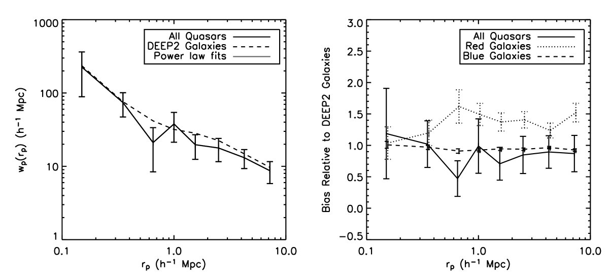
Figure 3.— Left: The projected cross-correlation function between SDSS and DEEP2 quasars and all DEEP2 galaxies is shown as a solid line, while the dashed line shows the auto-correlation function of DEEP2 galaxies within $\Delta z=0.1$ of the quasars (see text for details). Right: The solid line shows the relative bias between quasars and all DEEP2 galaxies as a function of scale, while the dotted (dashed) lines shows the relative bias between red (blue) galaxies and all galaxies in the DEEP2 data.

References

- Abazajian et al. (2003) Abazajian, K., et al. 2003, AJ, 126, 2081
- Abazajian et al. (2004) Abazajian, K., et al. 2004, AJ, 128, 502
- Abazajian et al. (2005) Abazajian, K., et al. 2005, AJ, 129, 1755–1759
- Adelberger & Steidel (2005) Adelberger, K. L., & Steidel, C. C. 2005, Accepted to ApJ (astro-ph/0505210)
- Bahcall, Schmidt, & Gunn (1969) Bahcall, J. N., Schmidt, M., & Gunn, J. E. 1969, ApJ, 157, L77
- Bahcall & Chokshi (1991) Bahcall, N. A., & Chokshi, A. 1991, ApJ, 380, L9
- Blanton et al. (2003) Blanton, M. R., et al. 2003, AJ, 125, 2276
- Boroson (2005) Boroson, T. 2005, AJ, 130, 381
- Boyle et al. (2000) Boyle, B. J., et al. 2000, MNRAS, 317, 1014
- Brown, Boyle, & Webster (2001) Brown, M. J. I., Boyle, B. J., & Webster, R. L. 2001, AJ, 122, 26
- Castander et al. (2001) Castander, F. J., et al. 2001, AJ, 121, 2331
- Churazov et al. (2005) Churazov, E., et al. 2005, MNRAS, 363, L91
- Coil et al. (2004a) Coil, A. L., et al. 2004a, ApJ, 609, 525
- Coil et al. (2006) Coil, A. L., et al. 2006, ApJ, 644, 671
- Coil et al. (2004b) Coil, A. L., Newman, J. A., Kaiser, N., Davis, M., Ma, C., Kocevski, D. D., & Koo, D. C. 2004b, ApJ, 617, 765
- Cole & Kaiser (1989) Cole, S., & Kaiser, N. 1989, MNRAS, 237, 1127
- Conroy, Wechsler, & Kravtsov (2006) Conroy, C., Wechsler, R. H., & Kravtsov, A. V. 2006, Submitted to ApJ (astro-ph/0512234)
- Constantin & Vogeley (2006) Constantin, A., & Vogeley, M. 2006, astro-ph/0601717
- Cooper et al. (2006) Cooper, M., et al. 2006, submitted to MNRAS (astro-ph/0603177)
- Cooper et al. (2005) Cooper, M. C., et al. 2005, ApJ, 634, 833
- Croom et al. (2004a) Croom, S., et al. 2004a, In ASP Conf. Ser. 311: AGN Physics with the Sloan Digital Sky Survey, p. 457
- Croom et al. (2002) Croom, S. M., et al. 2002, MNRAS, 335, 459
- Croom et al. (2004b) Croom, S. M., et al. 2004b, MNRAS, 349, 1397
- Croom et al. (2005) Croom, S. M., et al. 2005, MNRAS, 356, 415
- Croton et al. (2006) Croton, D. J., et al. 2006, MNRAS, 365, 11
- Davis et al. (2003) Davis, M., et al. 2003, Proc. SPIE, 4834, 161 (astro-ph 0209419)
- Davis & Peebles (1983) Davis, M., & Peebles, P. J. E. 1983, ApJ, 267, 465
- Davis, Gerke, & Newman (2004) Davis, M., Gerke, B. F., & Newman, J. A. 2004, In Proceedings of ”Observing Dark Energy: NOAO Workshop”, Mar 18-20, 2004
- Efstathiou et al. (1988) Efstathiou, G., Frenk, C. S., White, S. D. M., & Davis, M. 1988, MNRAS, 235, 715
- Faber et al. (2003) Faber, S., et al. 2003, Proc. SPIE, 4841, 1657
- Faber et al. (2006) Faber, S. M., et al. 2006, accepted to ApJ, astro-ph/0506044
- Ferrarese & Merritt (2000) Ferrarese, L., & Merritt, D. 2000, ApJ, 539, L9
- Fukugita et al. (1996) Fukugita, M., et al. 1996, AJ, 111, 1748
- Gebhardt et al. (2000) Gebhardt, K., et al. 2000, ApJ, 539, L13
- Gunn et al. (1998) Gunn, J. E., et al. 1998, AJ, 116, 3040
- Gunn et al. (2006) Gunn, J. E., et al. 2006, AJ, 131, 2332
- Haiman & Hui (2001) Haiman, Z., & Hui, L. 2001, ApJ, 547, 27
- Hall & Green (1998) Hall, P. B., & Green, R. F. 1998, ApJ, 507, 558
- Hamilton (1992) Hamilton, A. J. S. 1992, ApJ, 385, L5
- Hawkins et al. (2003) Hawkins, E., et al. 2003, MNRAS, 346, 78
- Hennawi et al. (2005) Hennawi, J., et al. 2005, Submitted to AJ (astro-ph/0504535)
- Hopkins et al. (2005a) Hopkins, P. F., et al. 2005a, ApJ, 625, L71
- Hopkins et al. (2005b) Hopkins, P. F., et al. 2005b, ApJ, 632, 81
- Kaiser (1984) Kaiser, N. 1984, ApJ, 284, L9
- Kaiser (1987) Kaiser, N. 1987, MNRAS, 227, 1
- Kauffmann & Haehnelt (2000) Kauffmann, G., & Haehnelt, M. 2000, MNRAS, 311, 576
- Kauffmann & Haehnelt (2002) Kauffmann, G., & Haehnelt, M. G. 2002, MNRAS, 332, 529
- Laurikainen & Salo (1995) Laurikainen, E., & Salo, H. 1995, A&A, 293, 683
- Lidz et al. (2006) Lidz, A., et al. 2006, Submitted to ApJ (astro-ph/0507361)
- Martini & Weinberg (2001) Martini, P., & Weinberg, D. H. 2001, ApJ, 547, 12
- Mo & White (1996) Mo, H. J., & White, S. D. M. 1996, MNRAS, 282, 347
- Myers et al. (2006) Myers, A. D., et al. 2006, ApJ, 638, 622
- Peebles (1980) Peebles, P. J. E. 1980. The Large-Scale Structure of the Universe, Princeton, N.J., Princeton Univ. Press
- Porciani, Magliocchetti, & Norberg (2004) Porciani, C., Magliocchetti, M., & Norberg, P. 2004, MNRAS, 355, 1010
- Richards et al. (2002a) Richards, G. T., et al. 2002a, AJ, 124, 1
- Richards et al. (2002b) Richards, G. T., et al. 2002b, AJ, 123, 2945
- Richstone et al. (1998) Richstone, D., et al. 1998, Nature, 395, A14
- Schiavon et al. (2006) Schiavon, R., et al. 2006, submitted to ApJL, astro-ph/0602248
- Schlegel et al. (2006) Schlegel, D. J., et al. 2006, in preparation
- Schneider et al. (2005) Schneider, D. P., et al. 2005, AJ, 130, 367
- Seldner & Peebles (1979) Seldner, M., & Peebles, P. J. E. 1979, ApJ, 227, 30
- Serber et al. (2006) Serber, W., Bahcall, N., Menard, B., & Richards, G. 2006, ApJ, in press (astro-ph/0601522)
- Sheth & Tormen (1999) Sheth, R. K., & Tormen, G. 1999, MNRAS, 308, 119
- Smith, Boyle, & Maddox (1995) Smith, R. J., Boyle, B. J., & Maddox, S. J. 1995, MNRAS, 277, 270
- Smith, Boyle, & Maddox (2000) Smith, R. J., Boyle, B. J., & Maddox, S. J. 2000, MNRAS, 313, 252
- Spergel et al. (2006) Spergel, D., et al. 2006, astro-ph/0603449
- Springel, Di Matteo, & Hernquist (2005) Springel, V., Di Matteo, T., & Hernquist, L. 2005, ApJ, 620, L79
- Stoughton et al. (2002) Stoughton, C., et al. 2002, AJ, 123, 485
- Vanden Berk et al. (2001) Vanden Berk, D. E., et al. 2001, AJ, 122, 549
- Vanden Berk et al. (2005) Vanden Berk, D. E., et al. 2005, AJ, 129, 2047
- Wake et al. (2004) Wake, D. A., et al. 2004, ApJ, 610, L85
- Willmer et al. (2006) Willmer, C., et al. 2006, accepted to ApJ, astro-ph/0506041
- Wyithe & Loeb (2005) Wyithe, J. S. B., & Loeb, A. 2005, ApJ, 621, 95
- Yan, White, & Coil (2004) Yan, R., White, M., & Coil, A. L. 2004, ApJ, 607, 739
- Yee & Green (1984) Yee, H. K. C., & Green, R. F. 1984, ApJ, 280, 79
- Yee & Green (1987) Yee, H. K. C., & Green, R. F. 1987, ApJ, 319, 28
- York et al. (2000) York, D. G., et al. 2000, AJ, 120, 1579