WMAP 3-year primordial power spectrum

Abstract

We constrain the form of the primordial power spectrum using Wilkinson Microwave Anisotropy Probe (WMAP) 3-year cosmic microwave background (CMB) data (+ other high resolution CMB experiments) in addition to complementary large-scale structure (LSS) data: 2dF, SDSS, Ly-$\alpha$ forest and luminous red galaxy (LRG) data from the SDSS catalogue. We extend the work of the WMAP team to that of a fully Bayesian approach whereby we compute the comparative Bayesian evidence in addition to parameter estimates for a collection of seven models: (i) a scale invariant Harrison-Zel’dovich (H-Z) spectrum; (ii) a power-law; (iii) a running spectral index; (iv) a broken spectrum; (v) a power-law with an abrupt cutoff on large-scales; (vi) a reconstruction of the spectrum in eight bins in wavenumber; and (vii) a spectrum resulting from a cosmological model proposed by Lasenby & Doran (2005) (L-D). Using a basic dataset of WMAP3 + other CMB + 2dF + SDSS our analysis confirms that a scale-invariant spectrum is disfavoured by between 0.7 and 1.7 units of log evidence (depending on priors chosen) when compared with a power-law tilt. Moreover a running spectrum is now significantly preferred, but only when using the most constraining set of priors. The addition of Ly-$\alpha$ and LRG data independently both suggest much lower values of the running index than with basic dataset alone and interestingly the inclusion of Ly-$\alpha$ significantly disfavours a running parameterisation by more than a unit in log evidence. Overall the highest evidences, over all datasets, were obtained with a power law spectrum containing a cutoff with a significant log evidence difference of roughly 2 units. The natural tilt and exponential cutoff present in the L-D spectrum is found to be favoured decisively by a log evidence difference of over 5 units, but only for a limited study within the best-fit concordance cosmology.

1 Introduction

The recent release of 3-year Wilkinson Microwave Anisotropy Probe (WMAP3; Hinshaw et al. 2007) data have provided precise measurements of temperature fluctuations in the cosmic microwave background (CMB). The accepted inflationary paradigm suggests that a primordial spectrum of almost scale-invariant density fluctuations produced during inflation went on to produce the observed structure in the CMB and that seen on large-scales in the current distribution of matter. Now, for the first time a purely scale invariant primordial spectrum is ruled out at $1\sigma$ (Spergel et al. 2007; Parkinson et al. 2006) in favour of a ‘tilted’ spectrum with $n<1$. The WMAP team have already attempted limited constraints on the form of the spectrum and Parkinson et al. (2006) have conducted a model selection study to ascertain the necessity of a tilt in the spectrum with the new data. In this paper we extend both studies to a suite of models covering a wide variety of possibilities based on both physical and observational grounds. We use a fully Bayesian approach to determine the model parameters and comparative evidence to ascertain which model the data actually prefers.

Our previous paper (Bridges et al., 2006) [Bridges06] used WMAP 1-year data (WMAP1; Bennett et al. 2003) to constrain the same set of models. These generalisations were motivated principally by observations of a decrement in power on large-scales from WMAP1 and a tilting spectrum on small-scales from high resolution experiments such as the Arcminute Cosmology Bolometer Array (ACBAR; Kuo et al. 2004), the Very Small Array (VSA ; Dickinson et al. 2004) and the Cosmic Background Imager (CBI; Readhead et al. 2004). With two more years observing time and improved treatment of systematic errors the decrement in power on large scales is now somewhat reduced, yet still evident in WMAP3 and is now constrained almost to the cosmic variance limit while the tilting spectrum on small-scales is now seen even without the aid of high-resolution small scale experiments, due to tighter constraints on the second acoustic peak. On physical grounds we test a broken spectrum caused perhaps by double field inflation (Barriga et al., 2001) and a spectrum predicted by Lasenby & Doran (2005) (L-D) naturally incorporating an exponential cutoff in power on large scales by considering the evolution of closed universes out of a big bang singularity, with a novel boundary condition that restricts the total conformal time available in the universe. We also aim to reconstruct the spectrum in a number of bins in wavenumber $k$.

2 Model Selection Framework

Bayesian model selection is now well established within the community as a reliable means of appropriately determining the most efficient parameterisation for a model, penalising any unecessary complication (Jaffe 1996, Drell et al. 2000, John & Narlikar 2002, Hobson et al. 2003, Hobson & McLachlan 2003, Slosar et al. 2003, Saini et al. 2004, Marshall et al. 2003, Niarchou et al. 2004, Basset et al. 2004, Mukherjee et al. 2006, Trotta 2007, Beltran et al. 2005, Bridges06). Recently much progress has been made in improving the speed and accuracy of evidence results (Parkinson et al., 2006) by implementing the method of Skilling (2004) known as nested sampling. In this paper we will employ our own implementation of this method (Shaw et al., 2007) to evaluate the evidence and use standard Markov Chain Monte Carlo (MCMC) to make parameter constraints.

2.1 Markov Chain Monte Carlo sampling

A Bayesian analysis provides a coherent approach to estimating the values of the parameters, $\mathbf{\Theta}$, and their errors and a method for determining which model, $M$, best describes the data, $\mathbf{D}$. Bayes theorem states that

$$P(\mathbf{\Theta}|\mathbf{D},M)=\frac{P(\mathbf{D}|\mathbf{\Theta},M)P(\mathbf{\Theta}|M)}{P(\mathbf{D}|M)},$$ (1)

where $P(\mathbf{\Theta}|\mathbf{D},M)$ is the posterior, $P(\mathbf{D}|\mathbf{\Theta},M)$ the likelihood, $P(\mathbf{\Theta}|M)$ the prior, and $P(\mathbf{D}|M)$ the Bayesian evidence. Conventionally, the result of a Bayesian parameter estimation is the posterior probability distribution given by the product of the likelihood and prior. In addition however, the posterior distribution may be used to evaluate the Bayesian evidence for the model under consideration.

We will employ a MCMC sampling procedure to explore the posterior distribution using an adapted version of the cosmoMC package (Lewis & Bridle, 2002) with four CMB datasets; WMAP3, ACBAR the VSA and CBI. We also include the 2dF Galaxy Redshift Survey (Percival et al., 2001), the Sloan Digital Sky Survey (Abazajian et al., 2003) and the Hubble Space Telescope (HST) key project (Freedman et al., 2001). These set of experiments comprise dataset I. Additionally we include two datasets which cover different scales and probe independent sources. The Ly-$\alpha$ forest (McDonald et al. 2006; McDonald et al. 2005) (which combined with dataset I makes up dataset II) comprises cosmological absorption by neutral hydrogen observed in quasar spectra in the intergalactic medium. It probes fluctuation scales that are small ($\sim$ Mpc) in comparison to the other datasets used at redshifts between 2-4 so that primordial information has not been erased by non-linear evolution. It thus provides a very useful complementary observation when constraining the form of the primordial spectrum. Previous authors (Viel, Haehnelt & Lewis 2006; Seljak et al. 2006) have already examined this dataset in conjunction with WMAP3 and others and found that most of the interesting results observed by Spergel et al. (2007), namely lowered scalar amplitude and a non-vanishing running index can be removed when Ly-$\alpha$ is included. Observations of luminous red galaxies (LRG) Tegmark et al. 2006 (when combined with dataset I becomes dataset III) consists of $>$ 46,000 galaxies taken from the full SDSS catalogue which represent a highly uniform galaxy sample containing only luminous early-types over the entire redshift range studied constituting an excellent tracer of large scale structure. Tegmark et al. (2006) recently detected baryonic acoustic oscillations in the matter power spectrum extracted from this dataset, providing a welcome confirmation of early universe physics in large scale structure data.

In addition to the primordial spectrum parameters, we parameterise each model using the following five cosmological parameters; the physical baryon density $\Omega_{b}h^{2}$; the physical cold dark matter density $\Omega_{c}h^{2}$; the curvature density $\Omega_{k}$; the Hubble parameter $h$ ($H_{0}=h\times 100\mbox{kms}^{-1}$) and the redshift of re-ionisation $z_{re}$.

2.2 Bayesian evidence and nested sampling

The Bayesian evidence is the average likelihood over the entire prior parameter space of the model:

$$\int\int{\mathcal{L}(\Theta_{\rm{C}},\Theta_{\rm{B}})P(\Theta_{\rm{C}})P(\Theta_{\rm{B}})}d^{N}\Theta_{\rm{C}}d^{M}\Theta_{\rm{B}},$$ (2)

where $N$ and $M$ are the number of cosmological and Bianchi parameters respectively. Those models having large areas of prior parameter space with high likelihoods will produce high evidence values and vice versa. This effectively penalises models with excessively large parameter spaces, thus naturally incorporating Ockam’s razor.

The method of nested sampling is capable of much higher accuracy than previous methods such as thermodynamic integration (see e.g. Beltran et al. 2005, Bridges06). due to a computationally more effecient mapping of the integral in Eqn. 2 to a single dimension by a suitable re-parameterisation in terms of the prior mass $X$. This mass can be divided into elements $dX=\pi(\mathbf{\Theta})d^{N}\mathbf{\Theta}$ which can be combined in any order to give say

$$X(\lambda)=\int_{\mathcal{L\left(\mathbf{\Theta}\right)>\lambda}}\pi(\mathbf{\Theta})d^{N}\mathbf{\Theta},$$ (3)

the prior mass covering all likelihoods above the iso-likelihood curve $\mathcal{L}=\lambda$. We also require the function $\mathcal{L}(X)$ to be a singular decreasing function (which is trivially satisfied for most posteriors) so that using sampled points we can estimate the evidence via the integral:

$$\mathcal{Z}=\int_{0}^{1}{\mathcal{L}(X)}dX.$$ (4)

Via this method we can obtain evidences with an accuracy 10 times higher than previous methods for the same number of likelihood evaluations.

A standard scenario in Bayesian model selection would require the computation of evidences for two models A and B. The difference of log-evidences $\ln\mathcal{Z}_{A}-\ln\mathcal{Z}_{B}$, also called the Bayes factor then quantifies how well A may fit the data when compared with model B. Jeffreys (1961) provides a scale on which we can make qualitative conclusions based on this difference: $\Delta\mbox{ln}\mathcal{Z}<1$ is not significant, $1<\Delta\mbox{ln}\mathcal{Z}<2.5$ significant, $2.5<\Delta\mbox{ln}\mathcal{Z}<5$ strong and $\Delta\mbox{ln}\mathcal{Z}>5$ decisive.

3 Primordial Power Spectrum Parameterisation

3.1 H-Z, power-law and running spectra

The early Universe as observed in the CMB is highly homogeneous on large scales suggesting that any primordial spectrum of density fluctuations should be close to scale invariant. The H-Z spectrum is described by an amplitude $A$ for which we assume a uniform prior of $[15,55]\times 10^{-8}$. Slow-roll inflation, given an exponential potential, predicts a slightly ‘tilted’ power-law spectrum parameterised as:

$$P(k)=A\left(\frac{k}{k_{0}}\right)^{n-1},$$ (5)

where the spectral index should be close to unity; we assume a uniform prior on $n$ of $[0.5,1.5]$; $k_{0}$ is the pivot scale (set to 0.05 Mpc^-1) of which $n$ and the amplitude $A$ are functions. For a generic inflationary potential we should also account for any scale dependence of $n(k)$ called running, so that to first order:

$$P(k)=A\left(\frac{k}{k_{0}}\right)^{n-1+(1/2)\ln(k/k_{0})(dn/d\ln k)},$$ (6)

where $dn/d\ln k$ is the running parameter $n_{run}$; for which we assume a uniform prior of $[-0.15,0.15]$.

The inclusion of WMAP3 in dataset I now places impressively tight constraints on all three models (see Fig. 1). The unexpected reduction in the value of the optical depth to reionisation, to $\tau\sim 0.09$ has had the effect of reducing the overall amplitude of the power spectrum, due to the well known $\tau$-$A$ degeneracy. This effect is noticeable in all cases but most particularly so in the H-Z spectrum in Fig. 1 (c). For the first time the single spectral index model now exhibits a constraint, to $1\sigma$, of $n_{s}=0.95\pm 0.02$ (see Fig. 1 (b)) excluding the possibility of a scale-invariant spectrum at this confidence level. Furthermore, a pure power-law (with $n_{run}=0$) is also excluded at the $1\sigma$ level with $n_{run}=-0.038\pm 0.030$ (Fig. 1 (a)).

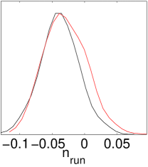
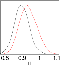
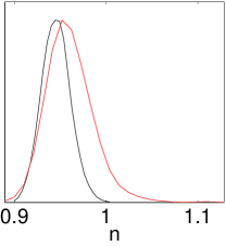
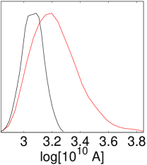
(a) Running

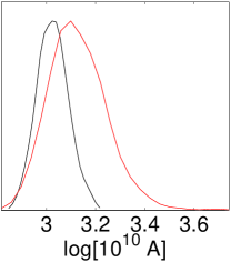
(b) Single-Index

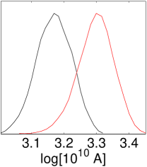
(c) H-Z

Figure 1: Marginalised parameter constraints with dataset I (black) for the H-Z, single-index and running models compared with our WMAP1 (Bridges06) analysis (red).

The addition of Ly-$\alpha$ data further increases constraints on all spectral parameters (see Fig. 2), particularly so on spectral running. While a scale invariant spectrum is also ruled out with this dataset ($n_{s}=0.96\pm 0.02$) a running spectrum is not preferred, with a constraint on $n_{run}=0.015\pm 0.015$ representing a doubling in accuracy over dataset I. A further tension exists between the amplitude of fluctuations as found using dataset I alone and when combined with Ly-$\alpha$, the latter preferring a much larger value of $\sigma_{8}$ and thus higher scalar fluctuation amplitude. Seljak et al. (2006) estimates this deviation to be at the $2\sigma$ level and treat it as a normal statistical fluctuation and not a sign of some unaccounted systematic flaw in either dataset. Since two independent analyses of WMAP3 + Ly-$\alpha$ and WMAP3 + LRG both suggest no significant running, a conservative conclusion is that the running observed with dataset I is simply a statistical anomaly albeit at close to 2$\sigma$.

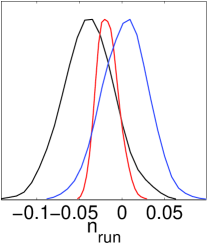
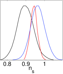
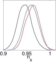
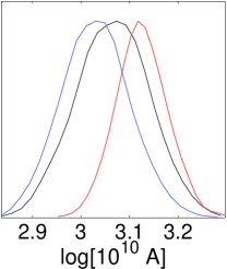
(a) Running

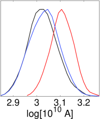
(b) Single-Index

(c) H-Z

Figure 2: Comparison of parameter constraints using dataset I (black) for the H-Z, single-index and running models with dataset II (red) and dataset III (blue).

3.2 Large scale cutoff

Confirmation by WMAP3 of the large-scale decrement in power at $\ell\sim 2$, close to the cosmic variance limit, supports the possibility of a spectrum with some form of cutoff. We reexamine the case of a sharp cutoff as did the WMAP team, parameterising the scale at which the power drops to zero, $k_{c}$ with a choice of prior $[0.0,0.0006]$ Mpc^-1 which was made to limit the study to regions up to $\ell\sim 6$ at which point an appreciable cutoff is no longer observed.

$$P(k)=\left\{\begin{array}[]{ll}0,&\mbox{$k<k_{c}$}\\ A\left(\frac{k}{k_{0}}\right)^{n-1},&\mbox{$k\geq k_{c}$}\end{array}\right.$$ (7)

Although this model $P(k)$ is not continuous, as the physical spectrum should be, it does give an upper limit on the average cutoff scale, which is useful when comparing for instance the L-D spectrum which does predict a form for the cutoff.

On small scales this spectrum behaves just as the single-index power law and so constraints on $A$ and $n$ are similar (see Fig. 3). Our WMAP1 constraint on $k_{c}$ showed a non-zero likelihood for a cutoff at $k=0$ i.e. no cutoff. This likelihood is marginally lower with WMAP3 presumably due to the higher amplitude of the $\ell=3$ multipole which was more heavily suppressed in WMAP1 observations. The peak in the likelihood encouragingly remains at around $k_{c}=2.8\times 10^{-4}$ Mpc^-1. The scale of this cutoff is much larger than anything probed by either Ly-$\alpha$ (in dataset II) or LRG (in dataset III), so neither dataset improves on this scale constraint (see Fig. 4).

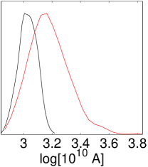
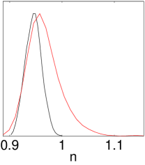
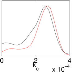
Figure 3: Marginalised parameter constraints for dataset I (black) for abrupt cutoff model compared with our WMAP1 (Bridges06) analysis (red).

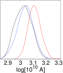
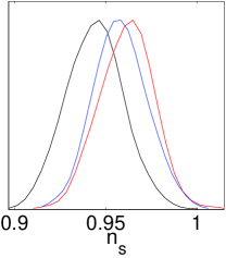
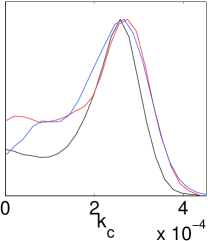
Figure 4: Comparison of cutoff constraints using dataset I (black), dataset II (red) and dataset III (blue).

3.3 Broken Spectrum

Multiple field inflation would produce a symmetry breaking phase transition in the early universe causing the mass of the inflaton field to change suddenly, momentarily violating the slow-roll conditions (Adams et al., 1997). The resultant primordial spectrum would be roughly scale invariant initially, followed by a sudden break lasting roughly 1 $e$-fold before returning to scale invariance. Because the slow-roll conditions are violated it is not trivial to calculate the form of the break, however a robust expectation is that it will be sharp as the field undergoing the phase transition evolves exponentially fast to its minimum (Barriga et al., 2001). We parameterise the spectrum as:

$$P(k)=\left\{\begin{array}[]{ll}A,&\mbox{$k\leq k_{s}$}\\ Ck^{\alpha-1},&\mbox{$k_{s}<k\leq k_{e}$}\\ B,&\mbox{$k>k_{e}$}\end{array}\right.,$$ (8)

where the values of $C$ and $\alpha$ are chosen to ensure continuity. Four power spectrum parameters were varied in this model: the ratio of amplitudes before and after the break $A/B$ with prior $[0.3,7.2]$; $k_{s}$ indicating the start of the break with prior $[0.01,0.1]$ Mpc^-1; $\ln(k_{e}/k_{s})$ to constrain the length of the break with prior $[0,4]$ and normalisation $A$ with prior $[14.9,54.6]\times 10^{-8}$. These represent a very conservative set of priors that allow the model a large degree of freedom in both the position of the break (which could occur anywhere from $k\sim 0.01$, well above any possible large scale cutoff) and the form, which could be extended, so as to mimic a tilted spectrum or occur as a sharp drop. In addition a prior that $k_{e}$ could not exceed 0.1 Mpc^-1 was imposed so that only a region well covered by the datasets used was explored.

In this parameterisation a scale invariant spectrum would have an amplitude ratio $A/B=1$ and a large value of $\ln(k_{e}/k_{s})$. Neither our WMAP1 analysis nor dataset I suggest this to be a plausible explanation (see Fig. 5) with a distinct drop in amplitude ($A/B\sim 1.2$) starting on scales below $k_{s}\sim 0.01$ Mpc^-1. The bimodal distribution in $\ln(k_{e}/k_{s})$ vs. $k_{s}$ observed with WMAP1 is preserved, though less pronounced, with dataset I. This implies a preference for both a sharp break at a single scale of $k\approx 0.04$ Mpc^-1 and an extended break begining at $k\approx 0.01$. A drop in power is clearly a crude way of approximating a tilted spectrum, so the extended break was an expected result. The sharp break, could be indicative of a some early universe physics or it could simply be as Bridle et al. (2003) suggest in their WMAP1 analysis, an artifact of the inclusion of the large scale structure datasets. The transition scale lies close to the point at which large scale structure data becomes statistically significant. Below this scale the WMAP data would disfavour a break and above it large scale structure data would. The inclusion of both Ly-$\alpha$ and LRG (see Fig. 6) data shifts the start of the break to larger scales (most pronounced with LRG), but simultaneously lowers the amplitude of the break, thus producing a more gradual extended slope, providing a better approximation to a tilted spectrum. Thus, our results do not conclusively suggest that a break does exist in the primordial spectrum, rather they seem only to confirm the need for a spectral tilt.

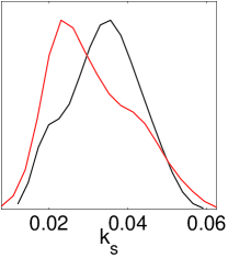
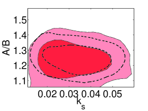
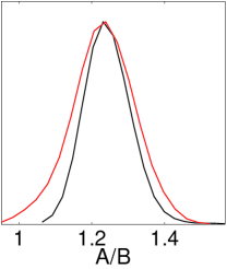
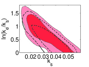
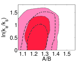
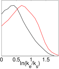
Figure 5: Marginalised 1D and 2D probability constraints for the broken spectrum model, for $k_{s}$, $\ln(k_{e}/k_{s})$ and $A/B$ for our WMAP1 (Bridges06) analysis (red) and dataset I (black). 2D constraints plotted with $1\sigma$ and $2\sigma$ confidence contours.

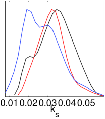
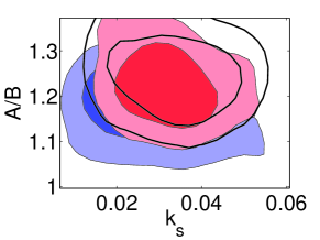
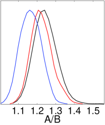
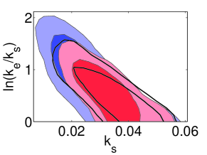
Figure 6: Marginalised 1D and 2D probability constraints for the broken spectrum model, for $k_{s}$, $\ln(k_{e}/k_{s})$ and $A/B$ for dataset I (black), dataset II (red) and dataset III (blue). 2D constraints plotted with $1\sigma$ and $2\sigma$ confidence contours.

3.4 Power spectrum reconstruction

Many previous attempts have been made to reconstruct the primordial spectrum directly from data: Wang 1994; Bridle et al. 2003; Shafieloo & Souradeep 2004; Sinha & Souradeep 2006; Tocchini-Valentini, Douspis & Silk 2005; Hannestad 2004; Bridges06. Most recently the WMAP team (Spergel et al., 2007) attempted to reconstruct it using a set of amplitude bins in $k$ using WMAP3 data alone. The method suffers from the natural side effect of imposing correlations between neighbouring bins and broadening other constraints. Therefore searching for features by this method is unreliable and difficult. However from a model selection viewpoint it does allow full freedom for the data to decide how many parameters are required of the model. Our parameterisation linearly interpolates between eight amplitude bins $a_{n}$ in $k$ on large scales between 0.0001 and 0.11 Mpc^-1 parameterised logarithmically with $k_{i+1}=2.75k_{i}$ so that

$$P(k)=\left\{\begin{array}[]{ll}\frac{(k_{i+1}-k)a_{i}+(k-k_{i})a_{i+1}}{k_{i+1}-k_{i}},&\mbox{$k_{i}<k<k_{i+1}$}\\ a_{n},&\mbox{$k\geq k_{n}$}\end{array}\right.$$ (9)

As expected an obvious tilt is discernible in our dataset I reconstruction (Fig. 7) the mean bin amplitudes deviating significantly from the best fit scale invariant spectrum at high $k$, not observable in our WMAP1 analysis. Though, within 1$\sigma$ limits a H-Z spectrum can still be fitted to both sets of data, however it would require a lower amplitude to accommodate the values at large $k$. No cutoff is observed as was hinted at in our WMAP1 analysis; however uncertainty at this scale is dominated by high cosmic-variance, making constraints inherently difficult. We find the addition of LRG data in dataset III provides little further constraint beyond that obtained from dataset I alone (see Fig. 8). The effect of including Ly-$\alpha$ data in dataset II is however, marked. Firstly the overall amplitude is lifted, owing to the larger $\sigma_{8}$ required by Ly-$\alpha$. Furthermore little obvious tilt is discernible in full agreement with our analysis in Sec. 3.1. Encouragingly similar features are seen in all three spectra such as the peaks at $0.003$ Mpc^-1 and $0.05$ Mpc^-1.

\psfrag{WMAP1}{ Bridges06 WMAP1 analysis}\psfrag{WMAP3}{ dataset I}\includegraphics[width=390.25534pt]{wmap3_binned.ps}

Figure 7: Reconstruction of the primordial power spectrum in 8 bands of $k$ (with $1\sigma$ errors) for dataset I (red) and our WMAP1 (Bridges06) analysis (yellow) compared with the best fit 1-year (dotted) and 3-year (filled) H-Z spectrum.

\psfrag{WMAP3}{ dataset I}\psfrag{Lya}{ dataset II}\psfrag{LRG}{ dataset III}\includegraphics[width=290.5246pt,angle={-90}]{wmap3_lya_lrg_binned_jan07.eps}

Figure 8: Reconstruction of the primordial power spectrum in 8 bands of $k$ (with $1\sigma$ errors) for dataset I (red), dataset II (magenta) and dataset III (green) compared with the best fit (black) H-Z spectrum from dataset I.

3.5 Closed universe Inflation

Lasenby & Doran (2005) arrived at a novel model spectrum by considering a boundary condition that restricts the total conformal time available in the Universe, and requires a closed geometry. The resultant predicted perturbation spectrum encouragingly contains an exponential cutoff (as previously suggested phenomenologically by Efstathiou 2003) at low $k$ that yields a corresponding deficit in power in the CMB power spectrum. The shape of the derived spectrum for a cosmology defined by $\Omega_{0}=1.04,\Omega_{b}h^{2}=0.0224,h=0.6,\Omega_{cdm}h^{2}=0.110$ was parameterised by the function:

$$P(k)=A(1-0.023y)^{2}(1-\exp(-(y+0.93)/0.47))^{2},$$ (10)

where $y=\ln\left(\frac{k}{H_{0}/100}\times 3\times 10^{3}\right)>-0.93$. However we do know this form to be fairly stable to changes in cosmology, particularly in the position of the cutoff. We therefore analyse this spectrum using dataset I, varying only the amplitude within the best fit ‘concordance’ cosmology found for the single index model in Sec. 3.1. As expected the amplitude is reduced when compared with our WMAP1 analysis ($A=27.1\pm 0.2$ Mpc^-1) due to the revised WMAP3 value for $\tau$. At small scales the spectrum then lies roughly in line with a tilted spectrum with $n_{s}\sim 0.96$ (see Fig. 9). For comparison the plot also shows the other best fit spectra (including the bimodality in the broken spectrum).

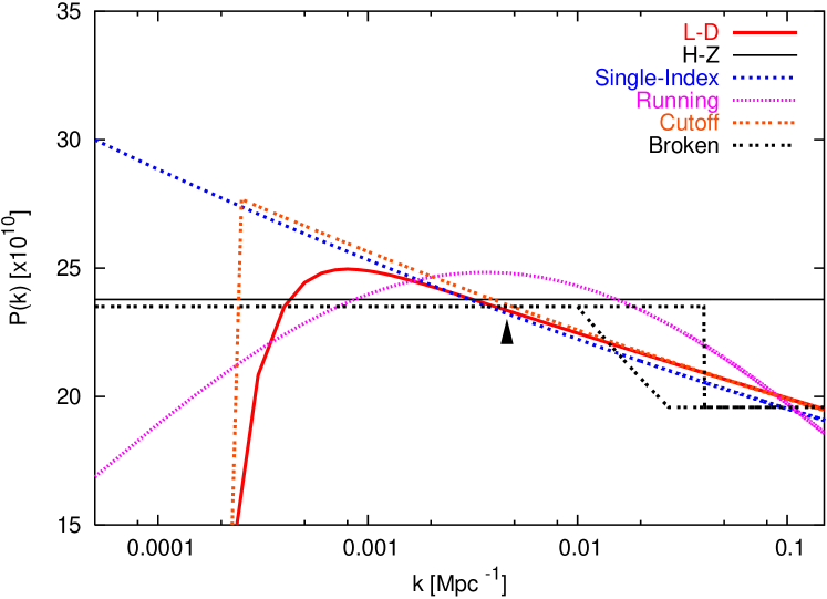
Figure 9: L-D spectrum (solid-red) shown with the WMAP3 best fitting H-Z (solid-black), single-index with a cutoff (dotted-orange), without (dotted-blue), a running index (dashed-pink) and broken (dotted-black).

3.6 Model Selection

We shall now turn to the fundamental inference. Which of the models considered best describes the current data? As with our WMAP1 analysis we perform the analysis in two stages to accommodate the L-D spectrum: the first, within the full parameter space including all models bar L-D, while the second was carried out within the fixed, best-fit single-index cosmology (as determined using dataset I) including L-D. While this artificial division may seem flawed it should be remembered that within this particular fixed cosmology the only spectrum that is favoured is that of the single-index model itself, any other models should only be penalised. We chose two sets of priors (see Table 1) on $n_{s}$ and $n_{run}$, the wider of which provides a very conservative range given the constraints available from current data. The results have been normalised to the single-index power law spectrum with wide priors.

Table 1: Priors placed on the principal primordial spectral parameters.

$A_{s}(\times 10^{-8})$	[15,55]
$n_{s}$ (wide priors)	[0.5,1.5]
$n_{s}$ (narrow priors)	[0.8,1.2]
$n_{run}$ (wide priors)	$[-0.15,0.15]$
$n_{run}$ (narrow priors)	$[-0.1,0.05]$

3.6.1 Full cosmological parameter space exploration

Our corresponding analysis of WMAP1 data was unable to make any conclusive model selection; with statistical uncertainty dominating results. With WMAP3 data and the method of nested sampling however we have arrived at a cusp in cosmological model selection. With dataset I, Table 2 confirms the disfavouring of a scale-invariant spectrum that we saw in the parameter constraints in Sec. 3.1, though not at a decisive level according to the Jeffrey’s scale. As expected from the parameter constraints a running spectrum is preferred, but only at a significant level if narrow priors are chosen on $n_{s}$ and $n_{run}$. Large scale power is suppressed in WMAP3 as it was in WMAP1, with little improvement in uncertainty: both datasets are almost cosmic-variance limited on these scales so a cutoff is preferred by a significant margin of over 2 units in log-evidence. The evidence in favour of a broken spectrum is likely only due to its mimicking of a tilted spectrum as opposed to modelling of an abrupt break.

Inclusion of Ly-$\alpha$ in dataset II confirms the conclusions drawn in Section 3.1, showing a significantly reduced evidence in favour of spectral running (with narrow priors), from a +1.2 with dataset I to -1.3, a significant evidence difference between the two datasets. Unsurprisingly all three data combinations exhibit significant evidences in favour of a spectral cutoff, due presumably in each case to the decrement in WMAP3 data alone.

Table 2: Differences of log-evidences with respect to single-index model (with the widest priors) using the full cosmological parameter space. [Note evidence comparisons can only be made between models using the same dataset.]

Model	datset I	+ Ly-$\alpha$	+ LRG
H-Z	$-0.7$ $\pm$ 0.3	$-0.1$$\pm$ 0.3	$-0.4$ $\pm$ 0.3
Single-Index (wide priors)	+0.0 $\pm$ 0.3	+0.0$\pm$ 0.3	+0.0 $\pm$ 0.3
Single-Index (narrow priors)	+1.0 $\pm$ 0.3	+0.2$\pm$ 0.3	+0.7 $\pm$ 0.3
Running (wide priors)	$-2.9$ $\pm$ 0.3	$-1.6$$\pm$ 0.3	$-1.8$ $\pm$ 0.3
Running (narrow priors on $n_{s}$)	+0.4 $\pm$ 0.3	$-0.7$$\pm$0.3	+1.7 $\pm$ 0.3
Running (narrow priors on $n_{run}$ & $n_{s}$)	+1.2 $\pm$ 0.3	$-1.3$$\pm$ 0.3	+1.0 $\pm$ 0.3
Cutoff	+2.3 $\pm$ 0.3	+1.7$\pm$ 0.3	+2.9 $\pm$ 0.3
Barriga	+1.0 $\pm$ 0.3	+1.2$\pm$ 0.3	+0.9 $\pm$ 0.3

3.6.2 Primordial parameter space exploration

The large preference in favour of a spectral cutoff and increasingly tight constraints on the universal geometry being marginally closed (a fact that is particularly reinforced when examining the LRG data Tegmark et al. (2006)), suggests that the L-D spectrum may provide a very good fit to current data. For the remainder of this analysis we will examine the L-D spectrum using dataset I only.

As with the WMAP1 analysis, dataset I, also prefers the L-D spectrum, now by a slightly larger log-evidence (see Table 3.), which according to Jeffreys’ scale now constitutes a decisive model selection. In Bridges06 we concluded that the ‘significant’ model detection was due to the form of the spectrum on large scales i.e. its exponential cutoff. However on small scales it behaves much like a tilted spectrum with slight running, a form we now know fits the data very well. Could it be that these small scale features are driving this model selection?

To test this hypothesis we have analysed three hybrid spectra, where we have divided the L-D spectrum about $k\approx 0.008$ Mpc^-1 (denoted by the arrow in Fig. 9) which corresponds loosely with the angular scale ($l=8$) where a cutoff ceases to be observed. We have then spliced both sections, about this point, with various single-index spectra at large or small scales. Model A combines a single-index spectrum below $k=0.0008$ Mpc^-1 with L-D thereafter; Model B: an exponential cutoff from L-D with a fixed single-index model ($n=0.94$) for $k>0.0008$ and Model C: as for B but with a varying single-index model.

The results (see Table 3) bear out our assertion; models A and B have roughly identical log-evidence values to the original L-D, demonstrating the data to be essentially indifferent to the presence of a cutoff. In comparison, model C is typically just as good as a power law spectrum (i.e. an evidence close to 0). This suggests that the L-D spectrum is attractive to the data as it naturally incorporates a tilt without the need to parameterise it. However the tilt present in the L-D spectrum ($n_{s}\sim 0.96$) does coincide well with the best fit values obtained in Sec. 3.1 for a power law spectrum (which are fairly invariant among the datasets I, II or III). This fact coupled with a significant evidence preference for a large scale spectral cutoff suggests the L-D spectrum does provide a uniquely good fit to current data.

Table 3: Differences of log-evidences (primordial parameters only) for all models with respect to the single-index models preferred cosmology: $\Omega_{0}=1.035,\Omega_{b}h^{2}=0.0221,h=0.58,\Omega_{cdm}h^{2}=0.112$, with our previous WMAP1 results for comparison.

Model	WMAP1 (Bridges06)	dataset I
Single-Index	+0.0 $\pm$ 0.5	+0.0 $\pm$ 0.2
L-D	+4.1 $\pm$ 0.5	+5.2 $\pm$ 0.2
L-D (A)	–	+5.0 $\pm$ 0.2
L-D (B)	–	+5.2 $\pm$ 0.2
L-D (C)	–	+0.9 $\pm$ 0.2

4 Conclusions

A scale-invariant spectrum is now largely disfavoured by the dataset I with a spectral index $n_{s}=0.95\pm 0.02$ deviating by at least 2$\sigma$ from $n_{s}=0$. Moreover a running spectrum ($n_{run}=-0.038\pm 0.030$) is now significantly preferred but only using the most constraining prior. The addition of Ly-$\alpha$ forest data improves all constraints but does not alter the preferred spectral tilt greatly. It does however, along with LRG data, suggest a significantly smaller running index ($n_{run}=-0.015\pm 0.015$, $n_{run}=0.01\pm 0.05$). This tension has previously been analysed by Seljak et al. (2006) who conclude that such discrepancies, even though at the 2$\sigma$ level are consistent with normal statistical fluctuations between datasets. A power law spectrum with a cutoff provides the best evidence fit in our full parameter space study with a significant evidence ratio of roughly 2 units across all three datasets. The similarity of this cutoff model with the L-D spectrum suggests the latter should also provide a very good fit. This is indeed borne out with decisively large evidence ratios within our limited primordial-only analysis.

References

- Abazajian et al. (2003) Abazajian K., et al., 2003, Astrophys. J., 126, 2081
- Adams et al. (1997) Adams J.A., Ross G.G. & Sarkar S., 1997, Nucl. Phys. B. 503, 405
- Barriga et al. (2001) Barriga J., Gaztanaga E., Santos M.G., Sarkar S., 2001, MNRAS, 324, 977
- Basset et al. (2004) Basset B.A., Corasaniti P.S., Kunz, M., Astrophys. J. Lett., 2004, 617, L1
- Beltran et al. (2005) Beltran M., Garcia-Bellido J., Lesgourgues J., Liddle A., Slosar A., 2005, Phys. Rev. D, 71, 063532
- Bennett et al. (2003) Bennett C.L., et al., 2003, Astrophys. J. Suppl., 148, 1
- Bridges et al. (2006) Bridges M., Lasenby A.N., Hobson, M.P., 2006, MNRAS, 369, 1123
- Bridle et al. (2003) Bridle S., Lewis A., Weller J., Efstathiou G., 2003, MNRAS, 342, L72
- Contaldi et al. (2003) Contaldi C.R., Peloso M., Kofman L., Linde A., 2003, J. Cosmol. Astropart. Phys., 7, 2
- Dickinson et al. (2004) Dickinson C. et al., 2004, MNRAS, 353, 732
- Drell et al. (2000) Drell P.S., Loredo T.J., Wasserman, I., 2000, Astrophys. J., 530, 593
- Efstathiou (2003) Efstathiou G., 2003, MNRAS, 346, 26
- Freedman et al. (2001) Freedman W.L., et al., 2001, Astrophys. J., 553, 47
- Hannestad (2004) Hannestad S., 2004, J. Cosmol. Astropart. Phys., 4, 2
- Hinshaw et al. (2007) Hinshaw G. et.al., 2007, Astrophys. J. Suppl., 170, 288
- Hobson et al. (2003) Hobson M.P., Bridle S.L., Lahav O., 2002, MNRAS, 335, 377
- Hobson & McLachlan (2003) Hobson M.P., McLachlan C., 2003, MNRAS, 338, 765
- Jaffe (1996) Jaffe A., 1996, Astrophys. J., 471, 24
- Jeffreys (1961) Jeffreys H., 1961, Theory of Probability, 3rd ed., Oxford University Press
- John & Narlikar (2002) John M.V., Narlikar J.V., 2002, Phys. Rev. D, 65, 043506
- Kuo et al. (2004) Kuo C.L. et al., 2004, Ap. J., 600, 32
- Lasenby & Doran (2005) Lasenby A.N., Doran, C., 2005, Phys.Rev. D 71, 063502
- Lewis & Bridle (2002) Lewis A. and Bridle S., 2002, Phys. Rev. D, 66, 103511
- Marshall et al. (2003) Marshall P.J., Hobson M.P., Slosar A., 2003, MNRAS, 346, 489
- McDonald et al. (2006) McDonald P., et al., 2006, Astrophys. J. Suppl., 163, 80-109
- McDonald et al. (2005) McDonald P., et al., 2005, Astrophys. J., 635, 761-783
- Mukherjee et al. (2006) Mukherjee, P. Parkinson D. Liddle, A., 2006, Astrophys. J., 638, L51-L54
- Mukherjee and Wang (2003) Mukherjee P. & Wang Y., 2003, Astrophys. J., 593, 38
- Niarchou et al. (2004) Niarchou A., Jaffe A., Pogosian L., 2004, Phys.Rev. D 69 063515
- Percival et al. (2001) Percival W.J. et al., 2001, MNRAS, 327, 1297
- Readhead et al. (2004) Readhead A.C.S. et al., 2004, Astrophys. J.,, 609, 498–512
- Parkinson et al. (2006) Parkinson D., Mukherjee P., Liddle A.R., 2006, Phys. Rev. D., 73, 123523
- Saini et al. (2004) Saini T.D., Weller J., Bridle S.L., 2004, MNRAS, 348, 603
- Seljak et al. (2006) Seljak U., Slosar A., McDonald P., 2006, J. Cosmol. Astropart. Phys., 10, 14
- Skilling (2004) Skilling J., 2004, Bayesian Inference and Maximum Entropy Methods in Science and Engineering, Ed. R. Fisher et al., American Inst. Phys. conf. proc., 735, 395
- Slosar et al. (2003) Slosar A. et al., 2003, MNRAS, 341, L29
- Shafieloo & Souradeep (2004) Shafieloo, A., Souradeep, T., 2004, Phys. Rev. D, 70, 043523
- Shaw et al. (2007) Shaw J.R., Bridges M., Hobson M.P., 2007, MNRAS, 378, 1365-1370
- Sinha & Souradeep (2006) Sinha, R., Souradeep, T., 2006, Phys. Rev. D., 74, 043518
- Spergel et al. (2003) Spergel D.N. et al., 2003, Astrophys. J. Suppl., 148, 175
- Spergel et al. (2007) Spergel D.N. et al., 2007, Astrophys. J. Suppl., 170, 377
- Tegmark et al. (2006) Tegmark M. et al., 2006,Phys. Rev. D, 74, 123507
- Tocchini-Valentini et al. (2005) Tocchini-Valentini D., Douspis M., Silk J., 2005, MNRAS, 359, 31
- Trotta (2007) Trotta R., 2007, MNRAS, 378, 72
- Viel, Haehnelt & Lewis (2006) Viel M., Haehnelt M.G., Lewis A., 2006, MNRAS, 370, L51
- Wang (1994) Wang Y., 1994, Phys. Rev. D, 50, 6135