$m=1$ Ideal Internal Kink Modes in a Line-tied Screw Pinch

Abstract

It is well known that the radial displacement of the $m=1$ internal kink mode in a periodic screw pinch has a steep jump at the resonant surface where $\mathbf{k}\cdot\mathbf{B}=0$.Rosenbluth et al. (1973) In a line-tied system, relevant to solar and astrophysical plasmas, the resonant surface is no longer a valid concept. It is then of interest to see how line-tying alters the aforementioned result for a periodic system. If the line-tied kink also produces a steep gradient, corresponding to a thin current layer, it may lead to strong resistive effects even with weak dissipation. Numerical solution of the eigenmode equations shows that the fastest growing kink mode in a line-tied system still possesses a jump in the radial displacement at the location coincident with the resonant surface of the fastest growing mode in the periodic counterpart. However, line-tying thickens the inner layer and slows down the growth rate. As the system length $L$ approaches infinity, both the inner layer thickness and the growth rate approach the periodic values. In the limit of small $\epsilon\sim B_{\phi}/B_{z}$, the critical length for instability $L_{c}\sim\epsilon^{-3}$. The relative increase in the inner layer thickness due to line-tying scales as $\epsilon^{-1}(L_{c}/L)^{2.5}$.

I Introduction

Magnetohydrodynamic (MHD) kink instability in a screw pinch is of great interest and has been under intensive study for decades. In a periodic system the internal kink mode is unstable if the safety factor $q$ (for a cylinder with axial periodicity length $L$, $q\equiv 2\pi rB_{z}/LB_{\phi}$) drops below unity somewhere within the plasma and increases with radius. Unstable modes have helical symmetry, depending on $z$ and $\phi$ in the combination $kz\pm\phi$, and possess so-called resonant surfaces $r=r_{s}$, on which $\mathbf{k}\cdot\mathbf{B}=kB_{z}\pm B_{\phi}/r_{s}=0$; due to the periodicity, the resonant surfaces must also be rational surfaces (if $k=2n\pi/L$, then on $r=r_{s}$, $q=\pm 1/n$ is a rational number). The driver of the instability lies within $r_{s}$, and the radial component of the plasma displacement nearly vanishes outside it. It has been shown that the thin transition layer near $r_{s}$ predicted from linear theory corresponds to an infinite current sheet in finite amplitude theory, at least within the framework of reduced, ideal MHD.Rosenbluth et al. (1973) In a plasma with large but finite Lundquist number, the steepening of the current layer must trigger resistive energy release, and it has been suggested that this energy release corresponds to the sawtooth crash.

The kink instability has also been proposed as a cause of solar flares. In this scenario, the instability occurs in a force free coronal magnetic loop which emerges from the photosphere and is twisted by photospheric motions. The possibility of forming a thin current sheet via the kink mode is particularly interesting, because the Lundquist number $S$ in coronal loops is so high ($\sim 10^{10-12}$) as to otherwise effectively preclude fast resistive MHD processes. For this reason, the instability and its current sheet are also of interest for the coronal heating problem. Following Parker’s original suggestion,Parker (1972) many authors Galsgaard and Nordlund (1996); Longbottom et al. (1998); Ng and Bhattacharjee (1998); Mikić et al. (1989) have shown that random shuffling of the coronal magnetic fieldlines by photospheric motions progressively increases the current density, resulting in sporadic energy release. How these spatially intermittent currents are produced, and in particular whether MHD instability plays any role, remains unclear. The kink instability is an interesting possible model of energy buildup and release. Line-tied kinking has also been captured in laboratory experiments; a recent example was reported in Ref. Bergerson et al. (2006).

However, the theory of the kink mode developed for periodic plasma does not carry over to line-tied systems such as coronal loops in a straightforward manner. It is generally agreed that line-tying is stabilizing, in the sense that a system with periodic boundary conditions is more unstable than an identical system of the same length with line-tied boundary conditions. Stabilization arises from the extra tension force associated with the anchored footpoints. Roughly, the system should be stable if the Alfvén travel time along the cylinder is less than the inverse of the growth rate in a periodic system. The first quantitative analysis of the effect of line-tying on stability was given by Raadu,Raadu (1972) who minimized the energy of a restricted class of perturbations. However, there is a deeper issue. Eigenfunctions with helical symmetry cannot satisfy boundary conditions on surfaces of constant $z$. Therefore, the significance of rational surfaces in aperiodic systems is open to question. Nevertheless, numerical studies Lionello et al. (1998a, b); Gerrard and Hood (2003, 2004); Gerrard et al. (2004) have shown that when a line-tied flux tube is twisted by motions of its endpoints, it eventually kinks, and the kinked state has a thin current layer (whether it is a current singularity or not is very difficult to examine by a numerical calculation). On the other hand, it has been shown quite rigorously that current sheets with the simple ribbon topology found from kink theory cannot appear in line-tied magnetic fields as long as their endpoint motion is a smooth function of position.van Ballegooijen (1985); Cowley et al. (1997) Thus, the question of what sets the current density in a kinked, line tied system is still open to investigation.

The purpose of ths paper is to clarify the relationship between the periodic and line-tied kink instabilities. In particular, we address the formation of thin current layers in line tied systems. In a periodic system, the rational surfaces constitute a natural set of separatrices, where current sheets can form. In a line-tied configuration, the notion of rational surfaces is absent; as such, it is not clear a priori where a thin current layer or current sheet, if any, would form. The present study addresses this important issue. And the answer, in short, is that the steep gradient in a line-tied system will appear at the resonant surface corresponding to the fastest growing periodic mode in a infinitely long system. A detailed comparison between the periodic eigenmode and the line-tied eigenmode is made. Through the comparison, the effects of line-tying on the growth rate and the eigenfunction can be clarified.

We limit ourselves to the linearized problem in this study, and leave the nonlinear problem to future work. This paper is organized as follows. Sec. II give the details of the model and the governing linearized equations. Sec. III presents the main results: comparsion of the periodic eigenmode and the line-tied one. We mostly concentrate on the fastest growing mode in both cases. Details are given for how the latter approach the former in the limit when the system length $L$ goes to infinity. An important quantity — the thickness of the internal layer — is found to follow a scaling law in that limiting process. Some other scaling laws regarding the critical length, the internal layer thickness and the mode localization along the axial direction at marginality are also found. We conclude and give a discussion in Sec. IV. Two appendices follow the main text. Appendix A gives the details of the numerical methods, and a semi-analytic calculation for the critical length and the growth rate is detailed in Appendix B.

II Model and Eigenmode Equations

We assume that the plasma pressure is negligible, $p=0$, and that the equilibrium plasma density $\rho=\mbox{const}$, for simplicity. In cylindrical coordinates $(r,\phi,z)$, the equilibrium magnetic field is

$$\mathbf{B}=B_{\phi}(r)\bm{\hat{\phi}}+B_{z}(r)\mathbf{\hat{z}},$$ (1)

which satisfies the force balance equation

$$-\frac{d}{dr}\left(\frac{B^{2}}{8\pi}\right)-\frac{B_{\phi}^{2}}{4\pi r}=0.$$ (2)

Assuming $e^{\gamma t}$ time dependence, the linearized ideal MHD equation can be expressed in terms of the Lagrangian displacement $\bm{\xi}$ as

$$\gamma^{2}\rho\bm{\xi}=\frac{1}{4\pi}(\nabla\times(\nabla\times(\bm{\xi}\times\mathbf{B})))\times\mathbf{B}+\frac{\nabla\times\mathbf{B}}{4\pi}\times(\nabla\times(\bm{\xi}\times\mathbf{B}))=0.$$ (3)

It is convenient to decompose the displacement $\bm{\xi}$ into the radial, perpendicular, and parallel components as

$$\bm{\xi}=\xi_{r}\mathbf{\hat{r}}+\xi_{\eta}\bm{\hat{\eta}}+\xi_{\parallel}\mathbf{\hat{b}},$$ (4)

where

$$\bm{\hat{\eta}}=(B_{z}\bm{\hat{\phi}}-B_{\phi}\mathbf{\hat{z}})/B,$$ (5)

and $\mathbf{\hat{b}}$ is the unit vector along the equilibrium magnetic field.

In the equilibrium, the $\phi$ direction is ignorable; we assume azimuthal dependence $e^{im\phi}$. Taking the $\mathbf{\hat{b}}$ component of Eq. (3) gives $\xi_{\parallel}=0$. The remaining two independent components of (3) are:

$$\gamma^{2}\xi_{r} = V_{A}^{2}\xi_{r}^{\prime\prime}+\frac{V_{Az}^{2}-V_{A\phi}^{2}}{r}\xi_{r}^{\prime}-\left(\frac{2V_{A\phi}V_{A\phi}^{\prime}}{r}+\frac{V_{A}^{2}}{r^{2}}\right)\xi_{r}+\left(V_{Az}\partial_{z}+\frac{imV_{A\phi}}{r}\right)^{2}\xi_{r}$$ (6)

$$-V_{A\phi}V_{A}\partial_{z}\xi_{\eta}^{\prime}-\left(\frac{2V_{A\phi}V_{A}}{r}+(V_{A}V_{A\phi})^{\prime}\right)\partial_{z}\xi_{\eta}+i\frac{mV_{A}V_{Az}}{r}\xi_{\eta}^{\prime}$$

$$+i\frac{m}{r}\left((V_{A}V_{Az})^{\prime}-\frac{V_{A}V_{Az}}{r}\right)\xi_{\eta},$$

$$\gamma^{2}\xi_{\eta}=-V_{A}V_{A\phi}\partial_{z}\left(\xi_{r}^{\prime}-\frac{\xi_{r}}{r}\right)+i\frac{mV_{A}V_{Az}}{r}\left(\xi_{r}^{\prime}+\frac{\xi_{r}}{r}\right)+iV_{A}^{2}\left(\partial_{z}^{2}-\frac{m^{2}}{r^{2}}\right)\xi_{\eta},$$ (7)

where primes denote $\partial_{r}$;$V_{Az}=B_{z}/\sqrt{4\pi\rho}$, $V_{A\phi}=B_{\phi}/\sqrt{4\pi\rho}$ , and $V_{A}=B/\sqrt{4\pi\rho}$, respectively.

In this work we are mostly interested in systems with a strong guide field, i.e., $V_{Az}\gg V_{A\phi}$. In that case, the kink mode is nearly incompressible and the growth rate is much smaller than the Alfvén frequency, i.e., $\gamma^{2}\ll V_{A}^{2}/a^{2}$, where $a$ is a characteristic perpendicular length scale of the flux tube. That means that large terms ($\sim O(V_{A}^{2}/a^{2})\left|\bm{\xi}\right|$) on the right-hand side (RHS) of Eqs. (6) and (7) nearly cancel each other; the small unbalanced remainders are balanced by the inertia term on the left-hand side (LHS). The cancellation of large terms could lead to a significant loss in accuracy when the eigenmode equations are solved numerically. To avoid that we reformulate the eigenmode equations as follows. Let

$$\xi_{\eta}=i\frac{rV_{Az}}{mV_{A}}\left(\xi_{r}^{\prime}+\frac{\xi_{r}}{r}\right)+\tilde{\xi_{\eta}},$$ (8)

where the first part on the RHS gives (approximate) incompressibility and $\tilde{\xi_{\eta}}$ is a small correction. Substituting (8) into the eigenmode equations, we have

$$\gamma^{2}\xi_{r} = V_{A\phi}^{2}\xi_{r}^{\prime\prime}+\left(\frac{V_{A\phi}^{2}}{r}+2V_{A\phi}V_{A\phi}^{\prime}\right)\xi_{r}^{\prime}+\frac{(1-m^{2})V_{A\phi}^{2}}{r^{2}}\xi_{r}$$ (9)

$$+\left(V_{Az}^{2}\partial_{z}^{2}+\left(\frac{2i(m^{2}-1)V_{A\phi}V_{Az}}{mr}+\frac{iV_{A\phi}^{3}}{mrV_{Az}}+\frac{i(V_{A\phi}^{2}-V_{Az}^{2})V_{A\phi}^{\prime}}{mV_{Az}}\right)\partial_{z}\right)\xi_{r}$$

$$-\frac{irV_{Az}V_{A\phi}}{m}\partial_{z}\xi_{r}^{\prime\prime}+\left(\frac{iV_{A\phi}^{3}}{mV_{Az}}+\frac{ir(V_{A\phi}^{2}-V_{Az}^{2})V_{A\phi}^{\prime}}{mV_{Az}}-\frac{4iV_{A\phi}V_{Az}}{m}\right)\partial_{z}\xi_{r}^{\prime}$$

$$-V_{A\phi}V_{A}\partial_{z}\tilde{\xi_{\eta}}^{\prime}-\left(\frac{2V_{A\phi}V_{A}}{r}-\frac{V_{A\phi}^{3}}{V_{A}r}+V_{A}V_{A\phi}^{\prime}\right)\partial_{z}\tilde{\xi_{\eta}}+i\frac{mV_{A}V_{Az}}{r}\tilde{\xi_{\eta}}^{\prime}$$

$$+i\frac{m}{r}\left(-\left(\frac{V_{Az}}{V_{A}}+\frac{V_{A}}{V_{Az}}\right)\frac{V_{A\phi}^{2}}{r}-\frac{V_{A}V_{A\phi}V_{A\phi}^{\prime}}{V_{Az}}-\frac{V_{A}V_{Az}}{r}\right)\tilde{\xi_{\eta}},$$

$$\gamma^{2}\left(-\frac{rV_{Az}}{mV_{A}}\left(\xi_{r}^{\prime}+\frac{\xi_{r}}{r}\right)+i\tilde{\xi_{\eta}}\right) = -iV_{A}V_{A\phi}\partial_{z}\left(\xi_{r}^{\prime}-\frac{\xi_{r}}{r}\right)-\frac{rV_{A}V_{Az}}{m}\partial_{z}^{2}\left(\xi_{r}^{\prime}+\frac{\xi_{r}}{r}\right)$$ (10)

$$+iV_{A}^{2}\left(\partial_{z}^{2}-\frac{m^{2}}{r^{2}}\right)\tilde{\xi_{\eta}}.$$

In this way the large terms on the RHS have been cancelled explicitly; all terms are $O(V_{A\phi}^{2}/a^{2})\left|\bm{\xi}\right|$ or smaller.

To make the numerical solution easier, we assume the existence of a conducting wall at $r=r_{0}$, which is made sufficiently far away that stability is only weakly affected. Two conducting plates at $z=\pm L/2$ anchor the magnetic field footpoints. Under these assumptions, the boundary conditions are $\xi_{r}|_{z=\pm L/2}=\tilde{\xi_{\eta}}|_{z=\pm L/2}=0$, and $\xi_{r}|_{r=r_{0}}=0$. The regularity condition at $r=0$ requires that $\xi_{r}\sim r^{|m|-1}$ and $\tilde{\xi_{\eta}}\sim r^{|m|+1}$ as $r$ approaches zero.

III Numerical Solution of Eigenmode Equations

In this section we present the numerical solutions of the eigenmode equations. The numerical method is described in Appendix A. The model system we solve in this work has the following force free equilibrium profiles:

$$V_{A\phi}=\epsilon r\exp(-r^{2}/2),$$ (11)

$$V_{Az}=\sqrt{1+\epsilon^{2}(1-r^{2})\exp(-r^{2})}.$$ (12)

This simple system has only three free parameters: $\epsilon$, $L$, and $r_{0}$. We fix the conducting outer boundary at $r_{0}=5$, sufficiently far that it only weakly affects the stability and the eigenfunction. The parameter $\epsilon\sim V_{A\phi}/V_{Az}$ is usually a small parameter in tokamak and coronal loop applications; in this work we systematically explore the region $\epsilon\leq 1$. For a given equilibrium, we solve the eigenmode equations for different $L$. We are particularly interested in studying how the growth rate and the thickness of the internal layer vary with the system length $L$.

III.1 Periodic Solutions

Before going into the results for line-tied systems, we present the results of the corresponding periodic systems. These results will serve as references to the line-tied solutions.

The analytical theory of the $m=1$ ideal internal kink mode in the limit $\epsilon\ll 1$ is given by Rosenbluth, Dagazian, and Rutherford in Ref. Rosenbluth et al. (1973) (hereafter RDR). Key results relevant to the present study are summarized as follows: (1) For an unstable eigenmode with spatial dependence $\exp(ikz+im\phi)$, with $m=\pm 1$, the eigenfunction $\xi_{r}(r)$ has a steep gradient (the internal layer) at the resonant surface $r=r_{s}$, i.e., where $\mathbf{k}\cdot\mathbf{B}=kB_{z}+mB_{\phi}/r_{s}=0$. Outside of the internal layer, $\xi_{r}\simeq\xi_{a}=\mbox{const}$ for $r<r_{s}$ and $\xi_{r}\simeq 0$ for $r>r_{s}$. (2) The growth rate of the unstable mode is approximately (there is a misprint of a factor of two in the original paper)

$$\gamma\simeq-\frac{\pi}{\left|(\mathbf{k}\cdot\mathbf{V}_{A})^{\prime}\right|_{r_{s}}r_{s}^{3}}\int_{0}^{r_{s}}g_{1}dr,$$ (13)

where

$$g_{1}=k^{2}r(3k^{2}r^{2}V_{Az}^{2}+2kmrV_{Az}V_{A\phi}-V_{A\phi}^{2}).$$ (14)

(3) The solution within the internal layer is approximately

$$\xi_{r}\simeq\frac{1}{2}\xi_{a}\left(1-\frac{2}{\pi}\tan^{-1}\left(\frac{x\left|(\mathbf{k}\cdot\mathbf{V}_{A})^{\prime}\right|_{s}}{\gamma}\right)\right),$$ (15)

where $x\equiv r-r_{s}$.

Some scaling laws can be deduced from these results. First, we have $\gamma\propto\epsilon^{3}$ in the following sense. In the limit $\epsilon\ll 1$, $V_{Az}$ is approximately constant. If we vary $\epsilon$ and let $k\propto\epsilon$, the resonant surface will be approximately located at a fixed radius, and the growth rate $\gamma$ will be proportional to $\epsilon^{3}$, since $g_{1}\propto\epsilon^{4}$ and $\left|(\mathbf{k}\cdot\mathbf{V}_{A})^{\prime}\right|_{r_{s}}\propto\epsilon$. Likewise, the thickness of the internal layer is proportional to $\epsilon^{2}$. To be precise, we define the thickness of the internal layer $\Delta$ as the distance between the two radii where $\xi_{r}=(3/4)\xi_{a}$ and where $\xi_{r}=(1/4)\xi_{a}$. Eq. (15) gives

$$\Delta\simeq 2\gamma/\left|(\mathbf{k}\cdot\mathbf{V_{A}})^{\prime}\right|_{r_{s}}.$$ (16)

Hereafter we will use the subscript “$0$” to denote properties of or related to the fastest growing periodic mode: for a given equilibrium, the fastest growing mode appears at the wavenumber $k=k_{0}$, with the growth rate $\gamma=\gamma_{0}$, and the internal layer thickness $\Delta_{0}$. From the scaling laws we have $k_{0}\propto\epsilon$ , $\gamma_{0}\propto\epsilon^{3}$, and $\Delta_{0}\propto\epsilon^{2}$.

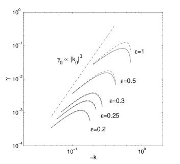
Figure 1: The growth rate $\gamma$ as a function of $k$, for different $\epsilon$. Solid lines are the growth rates calculated by the code, and dashed lines are the approximate growth rates calculated from Eq. (13). As expected, the agreement becomes better for smaller $\epsilon$. The dashdot line indicates the scaling law, $\gamma_{0}\propto\left|k_{0}\right|^{3}$.

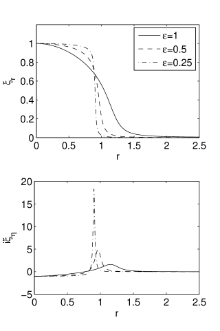
Figure 2: Periodic eigenfunctions of the fastest growing modes for $\epsilon=1$, $0.5$, $0.25$. The radial displacement $\xi_{r}$ has a jump at $r\simeq 1$. The jump becomes steeper, and the twist ($\xi_{\eta}$) becomes more localized, for smaller $\epsilon$. Note that only the solutions within $0\leq r\leq 2.5$ are shown; outside of that the solutions are vanishingly small. The eigenfunctions are normalized such that $\xi_{r}(0)=1$.

Figure 1 shows the growth rate $\gamma$ as a function of $k$, for different $\epsilon$. Solid lines denote the growth rate calculated by the code, and dashed lines are the approximate growth rate calculated from Eq. (13). As expected, the agreement becomes better for smaller $\epsilon$. For each $\epsilon$, the growth rate peaks at $k=k_{0}$, and the corresponding $\gamma_{0}$ follows the scaling law, $\gamma_{0}\propto\left|k_{0}\right|^{3}$, as indicated by the dashdot line. The numerical values of $k_{0}$, $\gamma_{0}$ , and $\Delta_{0}$ for different $\epsilon$ are summarized in Table 1. Figure 2 shows the eigenfunctions of the fastest growing modes for $\epsilon=1,$ $0.5$, $0.25$. The radial displacement $\xi_{r}$ of each shows a jump at $r\simeq 1$. The jump becomes steeper, and the twist ($\xi_{\eta}$) becomes more localized, for smaller $\epsilon$.

Notice that here the axial wavenumber $k$ is treated as a continuous parameter. This treatment actually corresponds to periodic eigenmodes in an infinitely long system. For a periodic system with a finite length $L$, the wavenumber $k$ is quantized as $k=2n\pi/L$, with integer $n$. As such, only a finite number of unstable modes are present in a finite length system.

III.2 Line-tied Solutions

We start by observing some general characteristics of the eigenmodes in line-tied systems, then move on to the scaling laws obtained from analyzing the numerical solutions. We focus only on the fastest growing mode for a given configuration in the first two sections. Higher harmonics are briefly discussed in section III.2.3.

III.2.1 General Observations

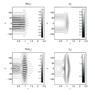
Figure 3: The fastest growing mode for the case $\epsilon=0.5$, $L=300$. The two panels on the left show the real part of $\xi_{r}$ and $i\xi_{\eta}$. The imaginary parts are not shown; they are similar to the real parts, only with different phases. The two panels on the right show the module of each component. The eigenfunctions are normalized such that $\xi_{r}|_{r=z=0}=1$.

Figure 3 shows the eigenfunctions of the fastest growing mode for $\epsilon=0.5$, $L=300$, which demonstrate some general characteristics observed throughout all the cases we have tried. The first thing to notice is that there are many oscillations along the $z$ direction. The wavelength is approximately the same as the corresponding fastest growing mode in the periodic case. Second, the radial displacement also has a jump at $r\simeq 1$, the same location as the jump of the fastest growing periodic mode. Third, the eigenmode is more or less localized to the center, rather than being broadened out to the whole $z$ domain, with an envelope $\sim\cos(\pi z/L)$, which seems to minimize the field line bending due to line-tying. In fact, the $\cos(\pi z/L)$ envelope is what Raadu used in his energy principle analysis,Raadu (1972) yet the numerical solutions suggest otherwise. We will come back to this issue later.

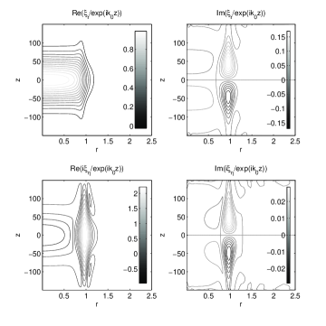
Figure 4: The fastest growing mode for $\epsilon=0.5$, $L=300$, divided by $\exp(ik_{0}z)$ to filter out the fast oscillations. The remaining “envelopes” are slowly varying functions along the $z$ direction.

Since the wavelength along $z$ is approximately the same as that of the fastest growing periodic mode, one may “filter out” the fast oscillations along $z$ by dividing the solutions by $\exp(ik_{0}z)$. The results are shown in Figure 4. The remaining “envelopes” of the eigenfunctions become slowly varying along the $z$ direction. This feature has been utilized into the choice of the basis functions of the numerical method, detailed in Appendix A. In short, instead of having to resolve the fast oscillations along $z$, we only need to resolve the slowly varying envelopes, therefore many fewer basis functions are needed.

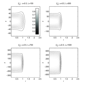
Figure 5: Contour plots of $\left|\xi_{r}\right|$for $\epsilon=0.5$, $L=150$, $300$, $700$, and $1500$. All solutions are normalized to $\xi_{r}|_{r=z=0}=1$. The contours correspond to $\left|\xi_{r}\right|=0.1$, 0.2, …, 0.8. As the system length becomes longer, the jump in $\left|\xi_{r}\right|$ becomes narrower, and the eigenfunction becomes broader along the $z$ direction. For a really long system, the $\cos(\pi z/L)$ envelope becomes a good approximation.

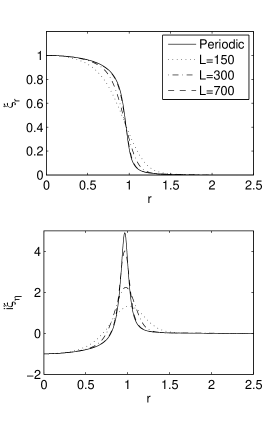
Figure 6: Eigenfunctions at the midplane, $z=0$, for different $L$, as compared to the fastest growing periodic eigenfunctions. $\epsilon=0.5$.

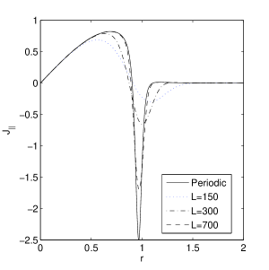
Figure 7: The perturbed parallel current at the midplane $z=0$. The thin current layer of the periodic case is smoothed in line-tied cases. The line-tied case approaches the periodic one as $L$ becomes larger.

Figure 5 shows the fastest growing mode for different $L$, with a fixed $\epsilon=0.5$. We observe that as $L$ becomes larger, the jump of the radial displacement becomes steeper, and the eigenfunction becomes broader along $z$. For a really long $L$, the envelope $\cos(\pi z/L)$ becomes a good approximation. Figure 6 shows the eigenfunctions at $z=0$, for various $L$, as compared to the periodic fastest growing mode. As $L$ becomes larger, the line-tied eigenfunctions at the midplane approach the periodic ones. For the case $L=1500$, which is not shown on the plot, the eigenfunctions at the midplane are virtually indistinguishable from the periodic ones. The parallel component of the perturbed current $J_{\parallel}\equiv\mathbf{\hat{b}}\cdot\nabla\times\nabla\times(\bm{\xi}\times\mathbf{V}_{A})$ at the midplane is shown in Figure 7. We see the thin current layer of the periodic solution is smoothed in line-tied cases. As the system length becomes longer, the line-tied solution approaches the periodic one. It should be pointed out, however, that the aspect ratio of these systems are much larger than in natural systems such as coronal loops.

Additional insight may be obtained by decomposing the eigenfunctions into Fourier harmonics. Because the wavelength along $z$ is approximately the same as the wavelength corresponds to $k_{0}$, we consider the following “shifted” Fourier decomposition:

$$\xi_{r}=\sum_{n=-\infty}^{\infty}\xi_{r}^{n}\exp\left(i\left(k_{0}+(2n-1)\pi/L\right)z\right).$$ (17)

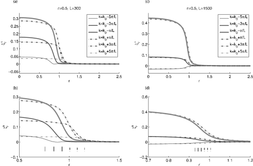
Figure 8: (a) The six most significant “shifted” Fourier components for the case $\epsilon=0.5$, $L=300$. (b) Expanded view of the jump at $r\simeq 1$. Vertical lines indicate the $\mathbf{k}\cdot\mathbf{B}=0$ surfaces corresponding to each $k$. (c) and (d) are the same as (a) and (b), for a longer system with $L=1500$.

Figure 8 (a) shows the six most significant Fourier components for the case $\epsilon=0.5$, $L=300$. We observe that they roughly form three pairs. The two components in each pair have approximately the same amplitude such that they nearly cancel each other at the ends, $z=\pm L/2$. However, the expanded view (b) about the jump at $r\simeq 1$ shows that each component has a jump at its own $\mathbf{k}\cdot\mathbf{B}=0$ surface, precluding cancellation within the narrow internal layer. As a result, many (actually an infinite number of) Fourier harmonics are needed to achieve a full cancellation at the ends. For a longer system, the distance between neighboring $\mathbf{k}\cdot\mathbf{B}=0$ surfaces becomes smaller. As shown in Figure 8 (c)(d), for the case $\epsilon=0.5$, $L=1500$, the two dominant components are nearly identical throughout the whole domain, and the components of other harmonics are very small. One may anticipate that in the limit $L\rightarrow\infty$ the solution is completely dominated by two components, which give a $z$ dependence $\sim\exp(ik_{0}z)\cos(\pi z/L)$. This is similar to the external kink mode solution calculated by Hegna Hegna (2004) and Ryutov et. al. Ryutov et al. (2004)

III.2.2 Scaling Laws and “Universalities”

It would be desirable if we could deduce some scaling laws from the numerical solutions. In particular, we are interested in how the internal layer thickness, the growth rate, the mode localization along $z$, the critical length for instability, etc., vary with $\epsilon$ or $L$. To be precise, let us define the quantities to be measured. The thickness $\Delta$ of the internal layer is measured at $z=0$. Let $\xi_{a}\equiv\left|\xi_{r}\right|_{r=0,z=0}$. The thickness $\Delta$ is defined as the distance between the radii where $\left|\xi_{r}\right|=(3/4)\xi_{a}$ and $\left|\xi_{r}\right|=(1/4)\xi_{a}$. The length $l$ of an eigenmode along $z$ is measured at $r=0$, and defined as the distance between the two points where $\left|\xi_{r}\right|=(1/2)\xi_{a}$. We use the subscript “$c"$ to denote properties associated with marginal stability: $L_{c}$ is the critical length for a given $\epsilon$; $l_{c}$ is the length, and $\Delta_{c}$ is the internal layer thickness, of the marginally stable eigenmode.

Table 2 summarizes $L_{c}$, $\Delta_{c}$, and $l_{c}$ for various $\epsilon$. For small $\epsilon$, we observe the following scaling laws: $L_{c}\propto 1/\epsilon^{3}$, $(\Delta_{c}-\Delta_{0})/\Delta_{0}\propto 1/\epsilon$, and $l_{c}/L_{c}\propto\epsilon$. The scaling $L_{c}\propto 1/\epsilon^{3}$ can be understood as follows. From a semi-analytic calculation (see Appendix B for details), we have an estimate for the critical length

$$L_{c}\simeq 2\left|V_{Az}\right|_{r_{s}}/\gamma_{0}$$ (18)

where $V_{Az}$ is evaluated at the resonant surface of the fastest growing periodic mode. For $\epsilon=$1, 0.5, 0.3, 0.25, 0.2, 0.15 this estimate gives $L_{c}\simeq$22.9, 130, 538, 910, 1746, 4079. Compared with the $L_{c}$ summarized in Table 2, the agreement is very good for small $\epsilon$. Since $V_{Az}\simeq\text{const}$ and $\gamma_{0}\propto\epsilon^{3}$ for small $\epsilon$, the scaling law follows. In the astrophysics literature, more often the critical twist of the magnetic field for a given flux tube length is considered. Let us consider the twist at the critical length:

$$\Delta\phi_{c}\propto\frac{L_{c}B_{\phi}}{rB_{z}}\propto\frac{1}{\epsilon^{2}}\propto L_{c}^{2/3}.$$ (19)

If we consider the flux tube length $L$ as given, and twist up the magnetic field to make it unstable, the critical twist scales as $L^{2/3}$.

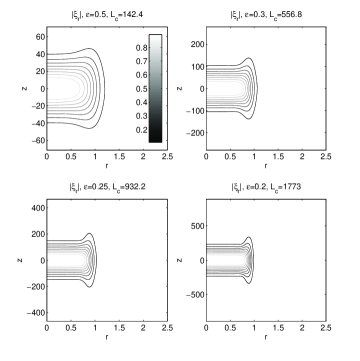
Figure 9: $\left|\xi_{r}\right|$ of the marginally stable eigenmodes for $\epsilon=0.5$, $0.3$, $0.25$, $0.2$. The eigenfunctions are normalized to $\xi_{r}|_{r=0,z=0}=1$. The contours correspond to $\left|\xi_{r}\right|=$0.1, 0.2, …, 0.8.

The quantity $(\Delta_{c}-\Delta_{0})/\Delta_{0}$ measures the relative increase in the internal layer thickness due to line-tying, and $l_{c}/L_{c}$ measures the localization along $z$ of the marginal mode. The scaling law $(\Delta_{c}-\Delta_{0})/\Delta_{0}\propto 1/\epsilon$ indicates that the increase in internal layer thickness is greater for smaller $\epsilon$, at marginal stability. And the scaling law $l_{c}/L_{c}\propto\epsilon$ indicates that the marginally stable mode becomes more and more localized along $z$ for smaller $\epsilon$. Figure 9 shows $\left|\xi_{r}\right|$ of the marginally stable eigenmodes for various $\epsilon$. The localization along $z$ is evident for smaller $\epsilon$. Note that the trend of localization along $z$ and broadening of the internal layer are reciprocal to each other. This is consistent with the understanding based on Fourier mode decomposition — localization along $z$ means a lot of Fourier harmonics are involved, that also means significant broadening of the internal layer.

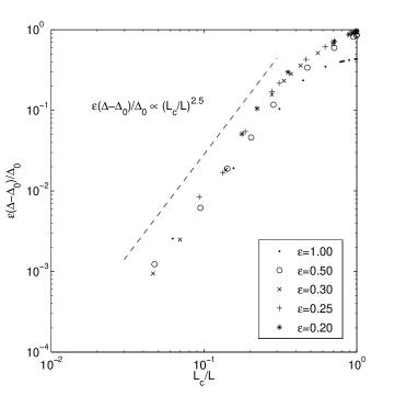
Figure 10: $\epsilon(\Delta-\Delta_{0})/\Delta_{0}$ as a function of $L_{c}/L$, for various $\epsilon$, in $\log-\log$ scale.

Let us now look at the internal layer thickness $\Delta$ as a function of $L$. We have already observed that $\Delta\rightarrow\Delta_{0}$ as $L\rightarrow\infty$. In an attempt to reveal some “universality”, we plot the functional dependence for various $\epsilon$, with a proper choice of variables and normalizations, on the same diagram. A natural choice of normalization for $L$ is with respect to $L_{c}$; therefore we choose $L_{c}/L$ as the horizontal axis. The choice for the vertical axis is not all that obvious. Since $(\Delta_{c}-\Delta_{0})/\Delta_{0}\propto 1/\epsilon$, we choose $\epsilon(\Delta_{c}-\Delta_{0})/\Delta_{0}$ as the vertical axis. With this choice of variables, the marginally stable solutions for different $\epsilon$ all appear roughly at the same point. Figure 10 shows the resulting plot in $\log-\log$ scale. We observe that all curves for different $\epsilon$ roughly coincide, and follow the scaling law $\epsilon(\Delta-\Delta_{0})/\Delta_{0}\propto(L_{c}/L)^{2.5}$. The curves deviate from the scaling law near marginality.

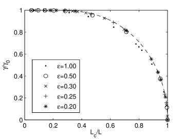
Figure 11: $\gamma/\gamma_{0}$ as a function of $L_{c}/L$, for various $\epsilon$. The dashed curve is analytic relation, Eq. (20).

Finally, let us look at how the growth rate varies with $L$. It is found that $\gamma\rightarrow\gamma_{0}$ as $L\rightarrow\infty$. We again try to plot the relationship between $\gamma$ and $L$ through a proper choice of variables. A natural choice is $L_{c}/L$ as the horizontal axis, and $\gamma/\gamma_{0}$ as the vertical axis. This choice brings all marginally stable modes to the same point $(1,0)$ on the plot. Figure 11 shows the resulting plot, for various $\epsilon$. Once again, all curves roughly coincide. The relation between $\gamma/\gamma_{0}$ and $L_{c}/L$ can be obtained by the semi-analytic calculation detailed in Appendix B as

$$\frac{L_{c}}{L}=\frac{\gamma/\gamma_{0}}{\tanh^{-1}(\gamma/\gamma_{0})},$$ (20)

which is in a good agreement with the numerical result. The line-tied growth rate $\gamma$ approaches the fastest periodic growth rate $\gamma_{0}$ rather quickly after the critical length is exceeded. For $L=2L_{c}$, about $95\%$ of the periodic growth rate is recovered.

III.2.3 Higher Harmonics

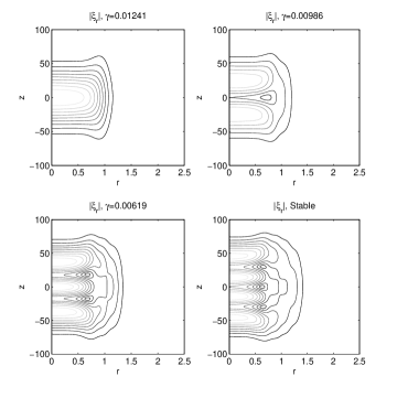
Figure 12: $|\xi_{r}|$ of four harmonics for the case $\epsilon=0.5$, $L=200$. Only three of them are unstable. The critical length is $L=142.4$.

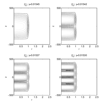
Figure 13: $|\xi_{r}|$ of four unstable modes for the case $\epsilon=0.5$, $L=1000$.

Thus far we have been focused on the fastest growing mode. Here we briefly discuss the higher harmonics. Figure 12 shows four harmonics of the case $\epsilon=0.5$, $L=200$. Since the length $L$ is not much longer than the critical length $L_{c}=142.4$, only three unstable modes are present. The kinking central column breaks into blobs for higher harmonics; the growth rate decreases with the increase in the number of blobs (hence more field line bending). Figure 13 shows the four most unstable modes for the system with the same $\epsilon=0.5$, but much longer $L=1000$. The higher harmonics still show the same general characteristics, but the growth rates of them are very close to the fastest one. In this case the physical significance of the fastest growing eigenmode becomes questionable, since those higher harmonics are likely to play an equally important role when the instability develops and reaches nonlinear saturation.

IV Summary and Discussion

In this paper we address the issue of the internal kink mode in a line-tied system, as compared to that in a periodic system. We find that the fastest growing internal kink mode in a line-tied system possesses a steep internal layer, as does its periodic counterpart. The internal layer locates at the resonant surface of the fastest growing periodic mode in an infinitely long system. Therefore, even though the notion of rational surfaces is absent in a line-tied system, we still have a rule of thumb as to where the current sheet would be. Line-tying decreases the growth rate and increases the internal layer thickness; only in the limit $L$ goes to infinity does the line-tied mode approach the periodic one.

In the small $\epsilon$ limit, the critical length can be estimated rather accurately using Eq. (18), and the dependence of the growth rate on $L$ is accurately represented by Eq. (20). Dimensionally, the critical length agrees with the physical picture that the system becomes unstable when the Alfvén travel time along the cylinder is longer than the inverse of the growth rate in a periodic system. A similar estimate can also be derived by applying the RDR asymptotic analysis to Raadu’s energy principle calculation, which gives

$$L_{c}\simeq\frac{\pi V_{A}|_{r_{s}}}{\gamma_{0}}.$$ (21)

Functionally this is similar to Eq. (18), but significantly overestimates the critical length by a factor of $\pi/2$. The reason is that Raadu assumed a $\cos(\pi z/L)$ envelope in his trial function, which is not a good approximation for the marginally stable mode, as the latter is highly localized to the center.

Several interesting scaling laws are deduced from the numerical solutions, most notably that $L_{c}\propto 1/\epsilon^{3}$, $l_{c}\propto 1/\epsilon^{2}$, $(\Delta_{c}-\Delta_{0})/\Delta_{0}\propto 1/\epsilon$, and $\epsilon(\Delta-\Delta_{0})/\Delta_{0}\propto(L_{c}/L)^{2.5}$. However, the computational overhead increases rather rapidly as one decreases $\epsilon$, due to the stringent scalings $\gamma_{0}\propto\epsilon^{3}$ and $\Delta_{0}\propto\epsilon^{2}$. As a result, the attainable parameter range of the numerical solution is limited. It would be desirable if the problem could be solved asymptotically in the limit $\epsilon\ll 1$, thereby the scaling laws can be “explained”. Our attempt at asymptotic solution only succeeds partially. We hope that the numerically found scaling laws can give some hint as to how the full analysis could be carried out.

As for application to realistic situations, Eqs. (18), (20), and the observed scaling laws are only valid in the small $\epsilon$ limit. For small $\epsilon$, the critical aspect ratio $L/a$ can easily go up to hundreds or thousands in order to make the flux tube unstable, and one may have trouble finding such a long flux tube in nature. Furthermore, for a naturally arising flux tube twisted up by footpoint motions, one can anticipate that the tube length will not be much longer than the critical length (or equivalently the twist will not be much greater then the critical one) before the instability sets in and completely alters the system. Therefore, even though the line-tied eigenfunction does approach the periodic one as $L\rightarrow\infty$, the physical significance is not clear. All these considerations point to the much more important nonlinear problem. Our next step will be to look at the nonlinear equilibrium after the instability, which will serve as a direct comparison to the nonlinear equilibrium given by RDR. Presently, there is still no consensus as to whether an infinitely thin current sheet or a current layer with finite thickness would form in a line-tied configuration. And we hope we can further clarify this issue.

Appendix A Numerical Method

We discretize the eigenmode equations by a Petrov-Galerkin schemeQuarteroni and Valli (1994). For a generalized eigenvalue problem of the form $\lambda\mathcal{L}_{1}u=\mathcal{L}_{2}u$, the weak form of the same system is $\lambda(\mathcal{L}_{1}u,w)=(\mathcal{L}_{2}u,w)$ for all $w$ in a suitable space of test functions, where $(\cdot,\cdot)$ denotes the inner product over the spatial domain. For our numerical method, we will approximate $u$ and $w$ with finite dimensional spaces, therefore turning the original partial differential eigenvalue equations into a matrix eigenvalue problem. In particular, we expand the variables $\xi_{r}$ and $i\tilde{\xi_{\eta}}$ as

$$\left[\begin{array}[]{c}\xi_{r}\\ i\tilde{\xi_{\eta}}\end{array}\right]=\sum_{\mu=1}^{2N_{r}}\sum_{\nu=1}^{N_{z}}a_{\mu\nu}\left[\begin{array}[]{c}\psi_{r}^{\mu}(r)\\ \psi_{\eta}^{\mu}(r)\end{array}\right]\phi^{\nu}(z).$$ (22)

Substituting this expression into the eigenmode equations, we then require the resulting equations to be satisfied identically when projected onto the $2N_{r}\times N_{z}$ basis functions of the test space

$$\left[\begin{array}[]{c}\bar{\psi_{r}^{\mu}}(r)\\ \bar{\psi_{\eta}^{\mu}}(r)\end{array}\right]\bar{\phi^{\nu}}(z).$$ (23)

For our convenience, we take

$$\left[\begin{array}[]{c}\bar{\psi_{r}^{\mu}}(r)\\ \bar{\psi_{\eta}^{\mu}}(r)\end{array}\right]=\left[\begin{array}[]{cc}r&0\\ -\frac{r^{2}V_{Az}}{mV_{A}}\left(\partial_{r}+\frac{1}{r}\right)&r\end{array}\right]\left[\begin{array}[]{c}\psi_{r}^{\mu}(r)\\ \psi_{\eta}^{\mu}(r)\end{array}\right],$$ (24)

$$\bar{\phi^{\nu}}(z)=\frac{\phi^{\nu}(z)}{\sqrt{1-(2z/L)^{2}}},$$ (25)

and the inner product is defined as

$$\left(\left[\begin{array}[]{c}f_{1}\\ g_{1}\end{array}\right],\left[\begin{array}[]{c}f_{2}\\ g_{2}\end{array}\right]\right)\equiv\int_{-L/2}^{L/2}dz\int_{0}^{r_{0}}dr(f_{1}f_{2}^{*}+g_{1}g_{2}^{*}).$$ (26)

The choice of $\bar{\psi_{r}^{\mu}}$ and $\bar{\psi_{\eta}^{\mu}}$ gives the correct form of energy integration in the $r$ direction, and the factor $1/\sqrt{1-(2z/L)^{2}}$ in $\bar{\phi^{\nu}}$ allows us to utilize the orthogonality of Chebyshev polynomials, which are used to construct the basis functions (see details below).

After lengthy calculations and integration by parts, the discretized approximation to the eigenmode equation can be written as

$$-\gamma^{2}M_{1}^{\alpha\beta}D_{0}^{\mu\nu}a_{\beta\nu}=\left(M_{2}^{\alpha\beta}D_{2}^{\mu\nu}+M_{3}^{\alpha\beta}D_{1}^{\mu\nu}+M_{4}^{\alpha\beta}D_{0}^{\mu\nu}\right)a_{\beta\nu},$$ (27)

where

$$M_{1}^{\alpha\beta} = -\int_{0}^{r_{0}}r\Bigg{[}A_{1}\frac{d\psi_{r}^{\alpha*}}{dr}\frac{d\psi_{r}^{\beta}}{dr}+A_{2}\psi_{r}^{\alpha*}\psi_{r}^{\beta}+A_{3}\left(\psi_{\eta}^{\alpha*}\frac{d\psi_{r}^{\beta}}{dr}+\psi_{\eta}^{\beta}\frac{d\psi_{r}^{\alpha*}}{dr}\right)$$ (28)

$$+A_{4}(\psi_{\eta}^{\alpha*}\psi_{r}^{\beta}+\psi_{\eta}^{\beta}\psi_{r}^{\alpha*})+\psi_{\eta}^{\alpha*}\psi_{\eta}^{\beta}\Bigg{]}dr,$$

with

$$A_{1}=\frac{r^{2}V_{Az}^{2}}{m^{2}V_{A}^{2}},$$ (29)

$$A_{2}=1-\frac{1}{m^{2}V_{A}^{2}}\left(V_{Az}^{2}-2rV_{A\phi}V_{A\phi}^{\prime}-2\frac{V_{A\phi}^{4}}{V_{A}^{2}}\right),$$ (30)

$$A_{3}=-\frac{rV_{Az}}{mV_{A}},$$ (31)

$$A_{4}=-\frac{V_{Az}}{mV_{A}};$$ (32)

$$M_{2}^{\alpha\beta} = \int_{0}^{r_{0}}\Bigg{[}A_{5}\frac{d\psi_{r}^{\alpha*}}{dr}\frac{d\psi_{r}^{\beta}}{dr}+A_{6}\psi_{r}^{\alpha*}\psi_{r}^{\beta}+A_{7}\left(\psi_{\eta}^{\alpha*}\frac{d\psi_{r}^{\beta}}{dr}+\psi_{\eta}^{\beta}\frac{d\psi_{r}^{\alpha*}}{dr}\right)$$ (33)

$$+A_{8}(\psi_{\eta}^{\alpha*}\psi_{r}^{\beta}+\psi_{\eta}^{\beta}\psi_{r}^{\alpha*})+A_{9}\psi_{\eta}^{\alpha*}\psi_{\eta}^{\beta}\Bigg{]}dr$$

with

$$A_{5}=\frac{r^{3}V_{Az}^{2}}{m^{2}},$$ (34)

$$A_{6}=\frac{m^{2}-1}{m^{2}}rV_{Az}^{2}+\frac{2rV_{A\phi}^{2}}{m^{2}}+\frac{2r^{2}V_{A\phi}V_{A\phi}^{\prime}}{m^{2}},$$ (35)

$$A_{7}=-\frac{r^{2}V_{A}V_{Az}}{m},$$ (36)

$$A_{8}=-\frac{rV_{A}V_{Az}}{m},$$ (37)

$$A_{9}=rV_{A}^{2};$$ (38)

$$M_{3}^{\alpha\beta} = \int_{0}^{r_{0}}i\Bigg{[}A_{10}\frac{d\psi_{r}^{\alpha*}}{dr}\frac{d\psi_{r}^{\beta}}{dr}+A_{11}\psi_{r}^{\alpha*}\psi_{r}^{\beta}+A_{12}\left(\psi_{\eta}^{\alpha*}\frac{d\psi_{r}^{\beta}}{dr}+\psi_{\eta}^{\beta}\frac{d\psi_{r}^{\alpha*}}{dr}\right)$$ (39)

$$+A_{13}(\psi_{\eta}^{\alpha*}\psi_{r}^{\beta}+\psi_{\eta}^{\beta}\psi_{r}^{\alpha*})\Bigg{]}dr,$$

with

$$A_{10}=\frac{2r^{2}V_{Az}V_{A\phi}}{m},$$ (40)

$$A_{11}=\frac{2(m^{2}-1)V_{A\phi}V_{Az}}{m},$$ (41)

$$A_{12}=-rV_{A\phi}V_{A},$$ (42)

$$A_{13}=V_{A}V_{A\phi};$$ (43)

$$M_{4}^{\alpha\beta}=\int_{0}^{r_{0}}\left[A_{14}\frac{d\psi_{r}^{\alpha}}{dr}\frac{d\psi_{r}^{\beta}}{dr}+A_{15}\psi_{r}^{\alpha}\psi_{r}^{\beta}+A_{16}\psi_{\eta}^{\alpha}\psi_{\eta}^{\beta}\right]dr,$$ (44)

with

$$A_{14}=-rV_{A\phi}^{2},$$ (45)

$$A_{15}=\frac{(1-m^{2})V_{A\phi}^{2}}{r},$$ (46)

$$A_{16}=-\frac{m^{2}V_{A}^{2}}{r};$$ (47)

and

$$D_{2}^{\mu\nu}=\int_{-L/2}^{L/2}\bar{\phi^{\mu}}^{*}\frac{d^{2}\phi^{\nu}}{dz}dz,$$ (48)

$$D_{1}^{\mu\nu}=\int_{-L/2}^{L/2}\bar{\phi^{\mu}}^{*}\frac{d\phi^{\nu}}{dz}dz,$$ (49)

$$D_{0}^{\mu\nu}=\int_{-L/2}^{L/2}\bar{\phi^{\mu}}^{*}\phi^{\nu}dz.$$ (50)

We have tried various basis functions. A straightforward choice satisfying boundary conditions and regularity conditions at $r=0$ based on Chebyshev polynomials would be

$$\left[\begin{array}[]{c}\psi_{r}^{\mu}(r)\\ \psi_{\eta}^{\mu}(r)\end{array}\right] = \left[\begin{array}[]{c}(r/r_{0})^{|m|-1}[T_{\mu}(2r/r_{0}-1)-1]\\ 0\end{array}\right]\,\,\,\,\,\text{when }\mu\leq N_{r},$$ (55)

$$\left[\begin{array}[]{c}\psi_{r}^{\mu}(r)\\ \psi_{\eta}^{\mu}(r)\end{array}\right]=\left[\begin{array}[]{c}0\\ (r/r_{0})^{|m|+1}T_{\mu-N_{r}-1}(2r/r_{0}-1)\end{array}\right]\,\,\,\,\text{when }\mu>N_{r},$$ (56)

and

$$\phi^{\nu}(z)=T_{\nu+1}(2z/L)-T_{\nu-1}(2z/L),$$ (57)

where $T_{n}$ denotes the Chebyshev polynomial of order $n$.Boyd (2001) This choice of basis functions works well, but a significant amount of basis functions are needed, as the eigenmode typically possesses a steep gradient at some radius $r=s$ and many oscillations along $z$. To remedy the steep gradient problem, we need to pack more resolution about $r=s$. This is implemented by successively applying three arctan/tan mappings, which are recommended in Ref. Boyd (2001), as follows: First we map $r\in[0,r_{0}]\rightarrow r_{1}\in[0,1]$ with $s\rightarrow 1/2$ by

$$r_{1}=\frac{2}{\pi}\tan^{-1}\left(a_{1}\tan\left(\frac{\pi}{2}\frac{r}{r_{o}}\right)\right),$$ (58)

with

$$a_{1}=\frac{1}{\tan\left(\frac{\pi}{2}\frac{s}{r_{0}}\right)}.$$ (59)

Then a second mapping from $[0,1]\rightarrow[0,1]$

$$r_{2}=\frac{1}{\pi}\tan^{-1}\left(a_{2}\tan\left(\pi\left(r_{1}-\frac{1}{2}\right)\right)\right)+\frac{1}{2}$$ (60)

is applied, which packs more resolution about $r_{1}=1/2$ (which is mapped into $r_{2}=1/2$), with larger $a_{2}$ for more packing. Finally, we map $r_{2}\in[0,1]\rightarrow r_{3}\in[0,1]$ with $1/2\rightarrow s^{\prime}$ by

$$r_{3}=\frac{2}{\pi}\tan^{-1}\left(a_{3}\tan\left(\frac{\pi}{2}r\right)\right),$$ (61)

with

$$a_{3}=\tan\left(\frac{\pi}{2}s^{\prime}\right).$$ (62)

In this mapping, $s^{\prime}$ can be any number between $0$ and $1$, but we usually choose some $s^{\prime}>1/2$. This is motivated by the observation that typically the eigenmode structure is rather trivial ($\simeq 0$) in the region $r>s$, therefore one can put less resolution there. The basis functions are then defined in terms of $r_{3}$ as

$$\left[\begin{array}[]{c}\psi_{r}^{\mu}\\ \psi_{\eta}^{\mu}\end{array}\right] = \left[\begin{array}[]{c}(r_{3})^{|m|-1}[T_{\mu}(2r_{3}-1)-1]\\ 0\end{array}\right]\,\,\,\,\,\text{when }\mu\leq N_{r},$$ (67)

and

$$\left[\begin{array}[]{c}\psi_{r}^{\mu}\\ \psi_{\eta}^{\mu}\end{array}\right]=\left[\begin{array}[]{c}0\\ (r_{3})^{|m|+1}T_{\mu-N_{r}-1}(2r_{3}-1)\end{array}\right]\,\,\,\,\text{when }\mu>N_{r}.$$ (68)

To resolve the many oscillations along z without too many basis functions, we use the observation that the fastest growing mode, upon dividing by $e^{ik_{0}z}$ with $k_{0}$ being the wave number of the fastest growing mode in the corresponding infinite system, yields a smooth function with length scales $\sim L$. This suggests that one may use

$$\phi^{\nu}(z)=e^{ik_{0}z}(T_{\nu+1}(2z/L)-T_{\nu-1}(2z/L))$$ (69)

as the basis functions. This proves to be very efficient.

The integration along $r$ is carried out numerically by Gaussian quadrature. The integration along $z$ can be done analytically,Mason and Handscomb (2002) which gives

$$D_{0}^{\mu\nu}=\frac{L\pi}{2}\left[\begin{array}[]{cccccc}3/2&0&-1/2\\ 0&1&0&-1/2\\ -1/2&0&1&0&\ddots\\ &-1/2&0&\ddots&\ddots\\ &&\ddots&\ddots\end{array}\right],$$ (70)

$$D_{1}^{\mu\nu}=\pi\left[\begin{array}[]{cccccc}0&1\\ -2&0&2\\ &-3&0&3\\ &&-4&0&\ddots\\ &&&\ddots&\ddots\end{array}\right]+ik_{0}D_{0}^{\mu\nu},$$ (71)

$$D_{2}^{\mu\nu}=\frac{2\pi}{L}\times\left\{\begin{array}[]{cc}-2\mu(\mu+1)&\mu=\nu\\ -4\mu&\text{$\mu<\nu$, $\nu-\mu$ even}\end{array}\right.+2ik_{0}\pi\left[\begin{array}[]{cccccc}0&1\\ -2&0&2\\ &-3&0&3\\ &&-4&0&\ddots\\ &&&\ddots&\ddots\end{array}\right]-k_{0}^{2}D_{0}^{\mu\nu}.$$ (72)

The resulting finite dimensional eigenvalue problem is then solved by a Jacobi-Davidson iteration method, which is described in detail in Ref. Sleijpen and Van Der Vorst (1996); Fokkema et al. (1998).

The growth rates of unstable modes are benchmarked with an initial-value MHD code, NIMROD;Sovinec et al. (2004) and the critical lengths for instability are also in good agreement with the results published in Ref. Van der Linden and Hood (1999). A periodic version of the code is also developed, in which spatio-temporal dependence of the form $\exp(ikz+im\phi+\gamma t)$ is assumed.

Appendix B Semi-Analytic Analysis of Line-tied Internal Kink

The linear analysis of the periodic internal kink modes in RDR goes as follows. First the eigenvalue problem is approximated by a single equation for $\xi_{r}$. The equation is then solved approximately in the internal layer and the outer region separately. Finally, asymptotic matching of the inner and the outer solutions gives the growth rate of the unstable mode. In this appendix, we try to extend the analysis to a line-tied system. An estimate for the critical length and the relation between the growth rate and the system length are derived. It should be pointed out though, that the analysis is not completely satisfactory. At certain point, we are forced to appeal to numerical work to validate certain steps. That is why we call it semi-analytic.

Following the steps of the analysis of RDR, first we have to derive a single equation for $\xi_{r}$. We start with the variational principle for the eigenvalue problem.Freidberg (1987) Assuming $m=\pm 1$, for a displacement $\bm{\xi}$, the energy variation can be written in term of $\xi_{r}$ and $\tilde{\xi_{\eta}}$ as

$$W(\bm{\xi}) = \int_{-L/2}^{L/2}dz\int_{0}^{r_{0}}dr\Bigg{[}r^{3}\left|\mathbf{V}_{A}\cdot\nabla\xi_{r}^{\prime}\right|^{2}+A_{6}\left|\partial_{z}\xi_{r}\right|^{2}-iA_{7}\left(\partial_{z}\tilde{\xi_{\eta}}^{*}\partial_{z}\xi_{r}^{\prime}-c.c.\right)$$ (73)

$$-iA_{8}\left(\partial_{z}\tilde{\xi_{\eta}}^{*}\partial_{z}\xi_{r}-c.c.\right)+A_{9}\left|\partial_{z}\tilde{\xi_{\eta}}\right|^{2}$$

$$-A_{12}\left(\tilde{\xi_{\eta}}^{*}\partial_{z}\xi_{r}^{\prime}+c.c.\right)-A_{13}\left(\tilde{\xi_{\eta}}^{*}\partial_{z}\xi_{r}+c.c.\right)-A_{16}\left|\tilde{\xi_{\eta}}\right|^{2}\Bigg{]}$$

and the inertia term can be written as

$$I(\bm{\xi}) = \int_{-L/2}^{L/2}dz\int_{0}^{r_{0}}dr\,r\Bigg{[}A_{1}\left|\xi_{r}^{\prime}\right|^{2}+A_{2}\left|\xi_{r}\right|^{2}-iA_{3}\left(\tilde{\xi_{\eta}}^{*}\xi_{r}^{\prime}-c.c.\right)$$ (74)

$$-iA_{4}\left(\tilde{\xi_{\eta}}^{*}\xi_{r}-c.c.\right)+\left|\tilde{\xi_{\eta}}\right|^{2}\Bigg{]},$$

where the coefficients $A_{1}$—$A_{16}$ are defined in Appendix A, and $c.c.$ denotes complex conjugate. The eigenvalue problem is equivalent to the following variational problem:Freidberg (1987)

$$\gamma^{2}=-\frac{W(\bm{\xi})}{I(\bm{\xi})},$$ (75)

and

$$\delta\frac{W(\bm{\xi})}{I(\bm{\xi})}=0.$$ (76)

Since $\tilde{\xi_{\eta}}$ is small for kink modes in the small $\epsilon$ limit, we may approximate $I(\bm{\xi})$ as

$$I(\bm{\xi})\simeq\int_{-L/2}^{L/2}dz\int_{0}^{r_{0}}dr\,r^{3}\left|\xi_{r}^{\prime}\right|^{2}.$$ (77)

That is, that $I(\bm{\xi})$ only weakly depends on $\tilde{\xi_{\eta}}$ ; therefore we may minimize $W(\bm{\xi})$ with respect to $\tilde{\xi_{\eta}}$ first in the variational problem (76). The minimization gives the following relation between $\xi_{r}$ and $\tilde{\xi_{\eta}}$:

$$(A_{9}\partial_{z}^{2}+A_{16})\tilde{\xi_{\eta}}=iA_{7}\partial_{z}^{2}\xi_{r}^{\prime}+iA_{8}\partial_{z}^{2}\xi_{r}-A_{12}\partial_{z}\xi_{r}^{\prime}-A_{13}\partial_{z}\xi_{r}.$$ (78)

Since $r\partial_{z}\sim ikr\sim\epsilon$, this shows that $\tilde{\xi_{\eta}}\sim\epsilon^{2}$; therefore the approximation (77) is self-consistent. Using Eq. (78) in (75) to eliminate as many $\tilde{\xi_{\eta}}$ as possible, we may write $W$ as

$$W(\bm{\xi}) = \int_{-L/2}^{L/2}dz\int_{0}^{r_{0}}dr\left(r^{3}\left|\mathbf{V}_{A}\cdot\nabla\xi_{r}^{\prime}\right|^{2}+A_{6}\left|\partial_{z}\xi_{r}\right|^{2}-A_{9}\left|\partial_{z}\tilde{\xi_{\eta}}\right|^{2}+A_{16}\left|\tilde{\xi_{\eta}}\right|^{2}\right).$$ (79)

To complete the minimization, we still have to solve (78) for $\tilde{\xi_{\eta}}$ in terms of $\xi_{r}$. This could formally be done in terms of the Green’s function, but let us proceed with the following approximation. We expand $W$ up to $O(\epsilon^{4})$. The term $A_{9}\left|\partial_{z}\tilde{\xi_{\eta}}\right|^{2}$ in the integrand is $O(\epsilon^{6})$ therefore is negligible; and from Eq. (78),

$$\tilde{\xi_{\eta}}=\left(iA_{7}\partial_{z}^{2}\xi_{r}^{\prime}+iA_{8}\partial_{z}^{2}\xi_{r}-A_{12}\partial_{z}\xi_{r}^{\prime}-A_{13}\partial_{z}\xi_{r}\right)/A_{16}+O(\epsilon^{4}).$$ (80)

After some algebra and integration by parts in $r$, we have

$$W = \int_{-L/2}^{L/2}dz\int_{0}^{r_{0}}dr\bigg{[}r^{3}\left|\mathbf{V}_{A}\cdot\nabla\xi_{r}^{\prime}\right|^{2}-r^{5}\left|\partial_{z}(\mathbf{V}_{A}\cdot\nabla\xi_{r}^{\prime})\right|^{2}+3r^{3}V_{Az}^{2}\left|\partial_{z}^{2}\xi_{r}\right|^{2}-rV_{A\phi}^{2}\left|\partial_{z}\xi_{r}\right|^{2}$$ (81)

$$+imV_{Az}V_{A\phi}r^{2}\left(r\partial_{z}\xi_{r}^{\prime*}\partial_{z}^{2}\xi_{r}-r\partial_{z}\xi_{r}^{*}\partial_{z}^{2}\xi_{r}^{\prime}+\partial_{z}^{2}\xi_{r}^{*}\partial_{z}\xi_{r}-c.c.\right)\bigg{]}+O(\epsilon^{6}).$$

Integration by parts in $z$ gives

$$\int_{-L/2}^{L/2}dz\int_{0}^{r_{0}}dr\,imV_{Az}V_{A\phi}r^{2}\left(r\partial_{z}\xi_{r}^{\prime*}\partial_{z}^{2}\xi_{r}-r\partial_{z}\xi_{r}^{*}\partial_{z}^{2}\xi_{r}^{\prime}-c.c.\right)\\ =\int_{0}^{r_{0}}dr\,imV_{Az}V_{A\phi}r^{2}\left(r\partial_{z}\xi_{r}^{\prime*}\partial_{z}\xi_{r}-c.c.\right)_{-L/2}^{L/2}.$$ (82)

This term may be negligible in Eq. (81), as one can estimate

$$\left(r\partial_{z}\xi_{r}^{\prime*}\partial_{z}\xi_{r}-c.c.\right)_{-L/2}^{L/2}:\int_{-L/2}^{L/2}dz\left(\partial_{z}^{2}\xi_{r}^{*}\partial_{z}\xi_{r}-c.c.\right)\sim 1:kL\sim\epsilon^{2}:1,$$ (83)

where in the last step we use the observed scaling law that to have unstable mode, $L>L_{c}\propto 1/\epsilon^{3}$. We may also neglect the second term in the integrand of Eq. (81), since

$$r^{5}\left|\partial_{z}(\mathbf{V}_{A}\cdot\nabla\xi_{r}^{\prime})\right|^{2}:r^{3}\left|\mathbf{V}_{A}\cdot\nabla\xi_{r}^{\prime}\right|^{2}\sim k^{2}r^{2}:1\sim\epsilon^{2}:1.$$ (84)

Therefore $W$ can be further simplified to

$$W \simeq \int_{-L/2}^{L/2}dz\int_{0}^{r_{0}}dr\bigg{[}r^{3}\left|\mathbf{V}_{A}\cdot\nabla\xi_{r}^{\prime}\right|^{2}+3r^{3}V_{Az}^{2}\left|\partial_{z}^{2}\xi_{r}\right|^{2}-rV_{A\phi}^{2}\left|\partial_{z}\xi_{r}\right|^{2}$$ (85)

$$+imV_{Az}V_{A\phi}r^{2}\left(\partial_{z}^{2}\xi_{r}^{*}\partial_{z}\xi_{r}-c.c.\right)\bigg{]}.$$

Now we have the expressions for the energy $W$ and the inertia $I$ in terms of $\xi_{r}$ alone, Eqs. (85) and (77). We may now substitute the expressions into the variational principle (76) to obtain an single partial differential equation which approximates the full eigenvalue problem. There is a subtle point here. The form of the approximate $W$ requires four boundary conditions for $\xi_{r}$ in the $z$ direction. Two apparent ones are the line-tied boundary conditions $\xi_{r}|_{z=\pm L/2}=0$. A possible choice of another two boundary conditions is $\partial_{z}\xi_{r}|_{z=\pm L/2}=0$, which makes all boundary terms vanish when turning Eq. (76) into a partial differential equation through integration by parts. Assuming that, the approximate eigenvalue equation is

$$\left(r^{3}(-\gamma^{2}+(\mathbf{V}_{A}\cdot\nabla)^{2})\xi_{r}^{\prime}\right)^{\prime}+\left(3r^{3}V_{Az}^{2}\partial_{z}^{4}+2imr^{2}V_{Az}V_{A\phi}\partial_{z}^{3}+rV_{A\phi}^{2}\partial_{z}^{2}\right)\xi_{r}=0.$$ (86)

It is hard to justify this particular choice of boundary conditions rigorously. In particular, it is not the same as requiring $\tilde{\xi_{\eta}}=0$ at the boundary (see Eq. (80)). Nonetheless, numerical solutions show that this new eigenvalue problem is indeed a good approximation to the original one in the small $\epsilon$ limit. As we will see, it turns out that $\xi_{r}$ is vanishingly small within the boundary layers near $z=\pm L/2$, therefore indeed $\partial_{z}\xi_{r}|_{z=\pm L/2}\simeq 0$.

One nice feature of Eq. (86) is that, if we consider a periodic problem by letting $\partial_{z}\rightarrow ik$, the approximate equation of RDR is recovered. This allows us to apply a similar asymptotic technique to the present problem. Motivated by the numerical solution, let us write the eigenfunction as $\xi_{r}(r,z)=h(r,z)e^{ik_{0}z}$, where $k_{0}$ is the wavenumber of the fastest growing periodic mode, $e^{ik_{0}z}$ is the fast oscillating part, and $h(r,z)$ is the envelope slowly varying along the $z$ direction. Substituting this into the energy Eq. (85), the dominant term in the integrand is the positive definite $r^{3}\left|\mathbf{V}_{A}\cdot\nabla\xi_{r}^{\prime}\right|^{2}=r^{3}\left|\left(V_{Az}\partial_{z}+i\mathbf{k}_{0}\cdot\mathbf{V}_{A}\right)h^{\prime}\right|^{2}\sim O(\epsilon^{2}),$ and all other terms are $O(\epsilon^{4})$. For an unstable mode, which requires $W<0$, we must have $h^{\prime}\simeq 0$ everywhere except where $\mathbf{k}_{0}\cdot\mathbf{V}_{A}\simeq 0$. Therefore, the internal layer occurs at $r=r_{s}$, where $\mathbf{k}_{0}\cdot\mathbf{V}_{A}=0$; outside of the internal layer, $h(r,z)\simeq h_{0}(z)$ when $r<r_{s}$, and $h(r,z)\simeq 0$ when $r>r_{s}$.

Integrating Eq. (86) once along $r$, we have

$$\left(-\gamma^{2}+(\mathbf{V}_{A}\cdot\nabla)^{2}\right)\xi_{r}^{\prime}(r,z)=\\ -\frac{1}{r^{3}}\int_{0}^{r}d\bar{r}\left(3\bar{r}^{3}V_{Az}^{2}(\bar{r})\partial_{z}^{4}+2im\bar{r}^{2}V_{Az}(\bar{r})V_{A\phi}(\bar{r})\partial_{z}^{3}+\bar{r}V_{A\phi}^{2}(\bar{r})\partial_{z}^{2}\right)\xi_{r}(\bar{r},z).$$ (87)

Using $\xi_{r}(r,z)=h(r,z)e^{ik_{0}z}$ in Eq. (87), in the region $r<r_{s}$ we have

$$\left(-\gamma^{2}+\left(V_{Az}\partial_{z}+i\mathbf{k}_{0}\cdot\mathbf{V}_{A}\right)^{2}\right)h^{\prime}\simeq\frac{-h_{0}(z)}{r^{3}}\int_{0}^{r}g_{1}(\bar{r})d\bar{r},$$ (88)

where

$$g_{1}(r)=3k_{0}^{4}r^{3}V_{Az}^{2}+2mk_{0}^{3}r^{2}V_{Az}V_{A\phi}-k_{0}^{2}rV_{A\phi}^{2}.$$ (89)

In the RHS of Eq. (88) we make use of that $h(r,z)\simeq h_{0}(z)$ when $r<r_{s}$, and all derivatives on the envelope function are neglected as they are smaller compared to derivatives on the fast oscillating part $e^{ik_{0}z}$. Within the internal layer, we may assume that $\left(-\gamma^{2}+\left(V_{Az}\partial_{z}+i\mathbf{k}_{0}\cdot\mathbf{V}_{A}\right)^{2}\right)h^{\prime}$ is nearly independent of $r$; that is

$$\left(-\gamma^{2}+\left(V_{Az}\partial_{z}+i\mathbf{k}_{0}\cdot\mathbf{V}_{A}\right)^{2}\right)h^{\prime}=f(z).$$ (90)

The function $f(z)$ can be determined from the outer region by evaluating Eq. (88) at $r=r_{s}$:

$$f(z)=\frac{-h_{0}(z)}{r_{s}^{3}}\int_{0}^{r_{s}}g_{1}(r)dr.$$ (91)

Furthermore, $V_{Az}$ can be approximated by $V_{Az}(r_{s})$, and $\mathbf{k}_{0}\cdot\mathbf{V}_{A}\simeq(\mathbf{k}_{0}\cdot\mathbf{V}_{A})^{\prime}|_{r_{s}}x\simeq-V_{Az}(r_{s})\zeta^{\prime}(r_{s})x$, where $x\equiv r-r_{s}$ and

$$\zeta(r)\equiv-\frac{mV_{A\phi}}{rV_{Az}}.$$ (92)

Using these approximations, the governing equation within the internal layer is

$$\left(V_{Az}^{2}(\partial_{z}-i\zeta^{\prime}x)^{2}-\gamma^{2}\right)h^{\prime}=f(z).$$ (93)

Here $V_{Az}$ and $\zeta^{\prime}$ are evaluated at $r=r_{s}$. Eq. (93) can be formally solved using the Green’s function:

$$G(x;z,\bar{z})=\frac{e^{i\zeta^{\prime}x(z-\bar{z})}}{\gamma V_{Az}}\frac{\sinh\left(\gamma(z_{>}-L/2)/V_{Az}\right)\sinh\left(\gamma(z_{<}+L/2)/V_{Az}\right)}{\sinh\left(\gamma L/V_{Az}\right)},$$ (94)

where $z_{>}$ ($z_{<}$) is the larger (smaller) one of $z$ and $\bar{z}$. The solution is

$$h^{\prime}(x,z)=\int_{-L/2}^{L/2}G(x;z,\bar{z})f(\bar{z})d\bar{z}$$ (95)

The solution in the inner region has to match the solution in the outer region asymptotically. That requires that the jump in the inner solution as $x$ goes from $-\infty$ to $\infty$ be equal to the jump in the outer solution from the region $r<r_{s}$ to the region $r>r_{s}$:

$$\int_{-\infty}^{\infty}dx\,h^{\prime}(x,z)=-h_{0}(z).$$ (96)

The only $x$ dependence in $h^{\prime}(x,z)$ comes from the factor $e^{i\zeta^{\prime}x(z-\bar{z})}$ in the Green’s function, and the integration can be done easily:

$$\int_{-\infty}^{\infty}e^{i\zeta^{\prime}x(z-\bar{z})}dx=\frac{2\pi}{\left|\zeta^{\prime}\right|}\delta(z-\bar{z}).$$ (97)

Using Eqs. (97), (95), (94), and (91) in (96), the asymptotic matching condition is

$$\frac{2\pi}{\left|\zeta^{\prime}\right|}\frac{\sinh\left(\gamma(z-L/2)/V_{Az}\right)\sinh\left(\gamma(z+L/2)/V_{Az}\right)}{\gamma V_{Az}\sinh\left(\gamma L/V_{Az}\right)}\frac{\int_{0}^{r_{s}}g_{1}(r)dr}{r_{s}^{3}}h_{0}(z)=h_{0}(z).$$ (98)

It seems we are now in trouble. If we eliminate $h_{0}(z)$ from both sides, we end up requiring that a function of $z$ equals to unity, which is impossible. However, notice that in the limit $\gamma L/V_{Az}\gg 1$, we have

$$\frac{\sinh\left(\gamma(z-L/2)/V_{Az}\right)\sinh\left(\gamma(z+L/2)/V_{Az}\right)}{\gamma V_{Az}\sinh\left(\gamma L/V_{Az}\right)}\simeq-\frac{1}{2\gamma\left|V_{Az}\right|}$$ (99)

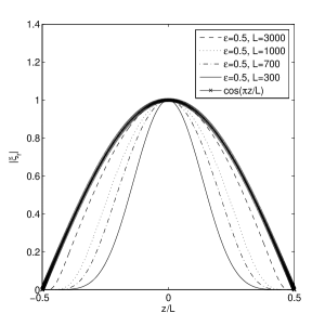
Figure 14: Envelope of $\xi_{r}$ at $r=0$ for the case $\epsilon=0.5$ with various $L$. The envelope function is confined to the central region and is vanishingly small within the boundary layers near the ends. The envelope function approaches $\cos(\pi z/L)$, which is shown as a reference, in the limit $L\rightarrow\infty$.

for most of the domain $z\in[-L/2,L/2]$, except in the two boundary layers of thickness $\sim V_{Az}/\gamma$ near both ends, where it drops to zero quickly. Therefore, as long as $h_{0}(z)$ is confined to the central region outside of the boundary layers, asymptotic matching is possible. Indeed, this qualitatively agrees with the observation on numerical solutions, exemplified in Fig. 14 for the case $\epsilon=0.5$ with different $L$. On the other hand, at marginal stability, $\gamma\rightarrow 0$, and

$$\frac{\sinh\left(\gamma(z-L/2)/V_{Az}\right)\sinh\left(\gamma(z+L/2)/V_{Az}\right)}{\gamma V_{Az}\sinh\left(\gamma L/V_{Az}\right)}\rightarrow\frac{\left(z-L/2\right)\left(z+L/2\right)}{LV_{Az}^{2}}.$$ (100)

In this limit, the “boundary layers” cover the whole domain, and we conclude that the marginal mode must be highly localized to the center. This is also in agreement with the numerical solutions.

Based on these observations, it may not be unreasonable to eliminate $h_{0}(z)$ from both side of Eq. (98), then approximate the left-hand side by its value at $z=0$. After some algebra, that gives the relation between $\gamma$ and $L$:

$$-\frac{\pi}{\left|\zeta^{\prime}V_{Az}\right|_{r_{s}}}\frac{\tanh\left(\gamma L/2\left|V_{Az}\right|_{r_{s}}\right)}{\gamma}\frac{\int_{0}^{r_{s}}g_{1}(r)dr}{r_{s}^{3}}=1.$$ (101)

Let us consider some limiting cases of Eq. (101) . In the limit $L\rightarrow\infty$,

$$\gamma=-\frac{\pi}{\left|\zeta^{\prime}V_{Az}\right|_{r_{s}}r_{s}^{3}}\int_{0}^{r_{s}}g_{1}(r)dr\equiv\gamma_{0}.$$ (102)

This essentially recovers the approximate periodic growth rate (13) since $(\mathbf{k}_{0}\cdot\mathbf{V}_{A})^{\prime}|_{r_{s}}\simeq-V_{Az}(r_{s})\zeta^{\prime}(r_{s})$. For marginal stability, let $\gamma\rightarrow 0$, we get an expression for the critical length

$$L_{c}=\frac{2\left|V_{Az}\right|_{r_{s}}}{\gamma_{0}}.$$ (103)

Finally, we can rewrite Eq. (101) in terms of $\gamma_{0}$ and $L_{c}$:

$$\frac{\gamma_{0}}{\gamma}\tanh\left(\frac{\gamma}{\gamma_{0}}\frac{L}{L_{c}}\right)=1.$$ (104)

In this appendix, we get good approximations for the critical length $L_{c}$ and the relation between $\gamma$ and $L$ without knowing the eigenmode structure along $z$. We also have no information about the thickness of the internal layer. This is not too surprising, as it is well known that getting a good approximation for the eigenfunction is more difficult than getting a good approximation for the eigenvalue. This can be understood from the variational principle, Eq. (76): Any deviation of the trial function from the true eigenfunction only leads to an error of second order in the eigenvalue. We learn from numerical solutions that the mode structure along $z$ and the internal layer thickness are correlated — the more a mode is localized in $z$, the thicker the internal layer is — therefore they must be solved all together. Attempts on extending the present analysis to resolve the mode structure have been unsuccessful. We hope this appendix can serve as a starting point for a more thorough analysis in the future.

$\epsilon$	$k_{0}$	$\gamma_{0}$	$\Delta_{0}$	$\left|k_{0}\right|/\epsilon$	$\gamma_{0}/\epsilon^{3}$	$\Delta_{0}/\epsilon^{2}$	$\gamma_{0}^{RDR}$	$\Delta_{0}^{RDR}$
1	-0.5287	$8.311\times 10^{-2}$	0.3908	0.5287	0.083	0.3909	$1.203\times 10^{-1}$	0.4945
0.5	-0.3121	$1.546\times 10^{-2}$	0.1217	0.6242	0.124	0.4868	$1.772\times 10^{-2}$	0.1305
0.3	-0.1970	$3.731\times 10^{-3}$	0.04458	0.6567	0.138	0.4953	$3.939\times 10^{-3}$	0.04569
0.25	-0.1658	$2.204\times 10^{-3}$	0.03091	0.6632	0.141	0.4946	$2.290\times 10^{-3}$	0.03152
0.2	-0.1337	$1.148\times 10^{-3}$	0.01977	0.6685	0.144	0.4943	$1.177\times 10^{-3}$	0.02005
0.15	-0.1009	$4.908\times 10^{-4}$	0.01111	0.6727	0.145	0.4938	$4.978\times 10^{-4}$	0.01122

Table 1: Summary of the wave number $k_{0}$, the growth rate $\gamma_{0}$, and the internal layer thickness $\Delta_{0}$ of the fastest growing mode in a periodic system. For smaller $\epsilon$, these quantities scale as expected. As a reference, $\gamma_{0}^{RDR}$ and $\Delta_{0}^{RDR}$ are the growth rate and thickness calculated by the Rosenbluth-Dagazian-Rutherford theory, Eqs. (13) and (15).

$\epsilon$	$L_{c}$	$\Delta_{c}$	$l_{c}$	$l_{c}/L_{c}$	$(\Delta_{c}-\Delta_{0})/\Delta_{0}$	$L_{c}\epsilon^{3}$	$\epsilon(\Delta_{c}-\Delta_{0})/\Delta_{0}$	$l_{c}/L_{c}\epsilon$
1	31.17	0.5605	15.64	0.502	0.4342	31.17	0.434	0.502
0.5	142.4	0.3304	44.97	0.316	1.715	17.8	0.858	0.632
0.3	556.8	0.1842	115.9	0.208	3.132	15.03	0.940	0.694
0.25	932.2	0.1502	164.8	0.177	3.859	14.57	0.965	0.707
0.2	1773	0.1153	262.4	0.148	4.832	14.18	0.966	0.740
0.15	4116	0.08371	468.5	0.114	6.535	13.89	0.980	0.759

Table 2: Summary of $L_{c}$, $\Delta_{c}$, and $l_{c}$ for various $\epsilon$, as well as the scaling laws they follow.

References

- Rosenbluth et al. (1973) M. N. Rosenbluth, R. Y. Dagazian, and P. H. Rutherford, Phys. Fluids 16, 1894 (1973).
- Parker (1972) E. N. Parker, Astrophys. J. 174, 499 (1972).
- Galsgaard and Nordlund (1996) K. Galsgaard and A. Nordlund, J. Geophy. Res. 101, 13445 (1996).
- Longbottom et al. (1998) A. W. Longbottom, G. J. Rickard, I. J. D. Craig, and A. D. Sneyd, Astrophys. J. 500, 471 (1998).
- Ng and Bhattacharjee (1998) C. S. Ng and A. Bhattacharjee, Phys. Plasmas 5, 4028 (1998).
- Mikić et al. (1989) Z. Mikić, D. D. Schnack, and G. van Hoven, Astrophys. J. 338, 1148 (1989).
- Bergerson et al. (2006) W. F. Bergerson, C. B. Forest, G. Fiksel, D. A. Hannum, R. Kendrick, J. S. Sarff, and S. Stambler, Phys. Rev. Lett. 96, 015004 (2006).
- Raadu (1972) M. A. Raadu, Solar Physics 22, 425 (1972).
- Lionello et al. (1998a) R. Lionello, D. D. Schnack, G. Einaudi, and M. Velli, Phys. Plasmas 54, 3722 (1998a).
- Lionello et al. (1998b) R. Lionello, M. Velli, G. Einaudi, and Z. Mikić, Astrophys. J. 494, 840 (1998b).
- Gerrard and Hood (2003) C. L. Gerrard and A. W. Hood, Solar Physics 214, 151 (2003).
- Gerrard and Hood (2004) C. L. Gerrard and A. W. Hood, Solar Physics 223, 143 (2004).
- Gerrard et al. (2004) C. L. Gerrard, A. W. Hood, and D. S. Brown, Solar Physics 222, 79 (2004).
- van Ballegooijen (1985) A. A. van Ballegooijen, Astrophys. J. 298, 421 (1985).
- Cowley et al. (1997) S. C. Cowley, D. W. Longcope, and R. N. Sudan, Physics Reports 283, 227 (1997).
- Hegna (2004) C. C. Hegna, Phys. Plasmas 11, 4230 (2004).
- Ryutov et al. (2004) D. D. Ryutov, R. H. Cohen, and L. D. Pearlstein, Phys. Plasmas 11, 4740 (2004).
- Quarteroni and Valli (1994) A. Quarteroni and A. Valli, Numerical Approximation of Partial Differential Equations (Springer-Verlag, 1994).
- Boyd (2001) J. P. Boyd, Chebyshev and Fourier Spectral Methods (Dover Publications, Inc., 2001), 2nd ed.
- Mason and Handscomb (2002) J. C. Mason and D. C. Handscomb, Chebyshev Polynomials (CRC Press LCC, 2002).
- Sleijpen and Van Der Vorst (1996) G. L. G. Sleijpen and H. A. Van Der Vorst, SIAM J. Matrix Anal. Appl. 17, 401 (1996).
- Fokkema et al. (1998) D. R. Fokkema, G. L. G. Sleijpen, and H. A. van der Vorst, SIAM J. Sci. Comput. 20, 94 (1998).
- Sovinec et al. (2004) C. R. Sovinec, A. H. Glasser, T. A. Gianakon, D. C. Barnes, R. A. Nebel, S. E. Kruger, D. D. Schnack, S. J. Plimpton, A. Tarditi, M. S. Chu, et al., J. Comput. Phys. 195, 355 (2004).
- Van der Linden and Hood (1999) R. A. M. Van der Linden and A. W. Hood, Astron. Astrophys. 346, 303 (1999).
- Freidberg (1987) J. P. Freidberg, Ideal Magnetohydrodynamics (Plenum Press, New York, 1987).