THE RISE TIME OF TYPE Ia SUPERNOVAE FROM THE SUPERNOVA LEGACY SURVEY¹

Abstract

We compare the rise times of nearby and distant Type Ia supernovae (SNe Ia) as a test for evolution using 73 high-redshift spectroscopically-confirmed SNe Ia from the first 2 years of the 5 year Supernova Legacy Survey (SNLS) and published observations of nearby SNe. Because of the “rolling” search nature of the SNLS, our measurement is approximately 6 times more precise than previous studies, allowing for a more sensitive test of evolution between nearby and distant SNe. Adopting a simple $t^{2}$ early-time model (as in previous studies), we find that the rest-frame $B$ rise times for a fiducial SN Ia at high and low redshift are consistent, with values $19.10^{+0.18}_{-0.17}\left(\mbox{stat}\right)\pm 0.2\left(\mbox{syst}\right)$ and $19.58^{+0.22}_{-0.19}$ days, respectively; the statistical significance of this difference is only 1.4 $\sigma$. The errors represent the uncertainty in the mean rather than any variation between individual SNe. We also compare subsets of our high-redshift data set based on decline rate, host galaxy star formation rate, and redshift, finding no substantive evidence for any subsample dependence.

1 INTRODUCTION

Type Ia supernovae (SNe Ia) have come to play a critical role in attempts to pin down the cosmological parameters. Their utility arises because they appear to constitute a class of high-quality standardizable candles. Considerable effort has been devoted by many groups to testing this assumption. Perhaps the most pernicious concern is that the properties of SNe Ia have evolved between the current epoch and $z\sim 0.3-1$, which characterizes most current “distant” supernova samples. One test for evolutionary effects is to compare the rise time, the time from explosion until maximum luminosity, of the nearby and distant samples. The early light-curve behavior should be influenced by the amount of ${}^{56}\mbox{Ni}$ synthesized in the explosion, as well as the opacity of the ejecta (Shigeyama et al., 1992; Branch, 1992; Khokhlov et al., 1993; Vacca & Leibundgut, 1996; Höflich et al., 1993, 1998; Domínguez et al., 2001). Changes in either of these, for example, due to changing progenitor metallicity with redshift, could affect the use of SNe Ia as standard candles. An evolutionary effect of 0.2 mag to $z=0.5$ would nullify the SN Ia evidence that the Universe is accelerating, and measuring $w$ to 10% requires that any effect be smaller than 0.04 mag. There are other routes to studying evolution with redshift: comparing SNe Ia in different host galaxy environments (Hamuy et al., 2000; Sullivan et al., 2003; Gallagher et al., 2005), and via detailed spectroscopic studies (Hook et al. 2005, Blondin et al. 2006, Bronder et al. 2006, in preparation). Neither approach has turned up any evidence of evolution.

The rise-time has implications for SNe Ia explosion models. Varying the rise time from 20 to 16 days at a fixed peak luminosity changes the implied amount of ⁵⁶Ni synthesized in the explosion by $-10\%$ (Contardo et al., 2000). Models of single white dwarf progenitor systems generally predict rise times in the range 13–19 days, while systems involving two white dwarfs allow for longer rise times because interaction with the disk of unaccreted material from the disrupted companion slows the diffusion of photons (Höflich & Khokhlov, 1996; Höflich et al., 2002).

The determination of the rise times has been the subject of some dispute. Historically, early-time, well-calibrated photometry of SNe Ia has been quite difficult to obtain. Some of the earliest studies of SNe Ia light-curve shapes examined the rise time (Pskovskii, 1984). Riess et al. (1999a, hereafter R99) presented early observations of a set of nearby SNe Ia detected 10–18 days before maximum $B$ luminosity. This data set was constructed primarily from unfiltered early detections, some from amateur observers. They transformed these observations to standard pass bands (in particular, $B$) using models of early-time SN Ia spectra and colors. They then considered various late-time light-curve parameterizations, concluding that the rise time for a fiducial SN Ia was $19.5\pm 0.2$ days. Riess et al. (1999b) compared this number with the preliminary analysis of Goldhaber et al. (2001, hereafter G01) for distant SNe Ia and concluded that the rise times differed by $2.5\pm 0.4$ days, a significance of $\sim 6\ \sigma$, and a clear signature of evolution.

Aldering et al. (2000, hereafter AKN00) argued that this comparison was based on analyses that had ignored the significant correlations between the light-curve parameters, and that taking these properly into account increased the errors on the rise time to $\pm 1.2$ days for the distant sample. They concluded that the significance of the difference was closer to $1.5\ \sigma$.

Our purpose here is not to revisit this controversy; rather, we present a new, significantly more precise ($\sim 6$ times) measurement of the high-redshift rise time and compare it with the value for nearby SNe. This has particular relevance because current SN projects place more stringent requirements on the standard-candle assumption. This paper presents measurements of the rise time from one such survey, the Supernova Legacy Survey (SNLS,Astier et al. (2006)). The design of this (and some other modern surveys) results in a dramatic increase in the amount of early-time photometry available when compared with previous generations of surveys, as detailed in §3.

We first describe the basic problem (§2), then present the data on which our measurement is based (§3), followed by a description of our analysis procedures (§4). Finally, we compare our measurements against nearby SNe Ia, as well as between different subsets of our data (§5).

2 RISE-TIME PARAMETERIZATION

In order to measure the rise time of our sample we require a mechanism for combining data from different SNe Ia, correcting for the differences in light-curve shape and peak flux, and a model for the early-time flux as a function of time. Considerable effort and ingenuity have been devoted to developing techniques for parameterizing SNe Ia light curves near and after maximum light (Riess et al. 1996, G01, Guy et al. 2005). Here we follow the stretch method as described in, for example, G01. The flux as a function of time after the rise-time region is represented as

$$f\left(t\right)=f_{0}\ \psi\left(\tau\right),$$ (1)

where $f_{0}$ is the flux at maximum, and $\psi$ is some normalized flux template appropriate to the passband under consideration. $\tau$ is the effective date defined by $\tau=\left(t-t_{\mbox{max}}\right)/s\left(1+z\right)$, where $t_{\mbox{max}}$ is the date of maximum flux in some arbitrary filter (usually $B$), $s$ is the stretch, and $z$ is the redshift. Conventionally, $s=1$ is defined to represent an average SN Ia. Once $s$, $f_{0}$, and $t_{\mbox{max}}$ are fited to the data, we can combine data from different SNe Ia by converting from observed epoch $t$ to $\tau$ and dividing by $f_{0}$ to normalize the flux values relative to each other. We must also apply a $K$-correction so that the resulting data are all expressed in the same rest-frame filter. Note that different observations from the same SN are correlated by this procedure, and that in addition estimates of the light-curve fit parameters are generally quite strongly correlated. We must take both into account in our analysis. For our purposes we limit the fit to this model to the “core” light curve between $-10<\tau<35$ days. The lower limit arises because we fit the rise-time model in this range, and we want to prevent the fit from suppressing unusual rise-time behavior. The upper limit arises because after this effective epoch the SNe Ia enter the so-called nebular phase, in which the stretch prescription no longer works (G01).

In the rise-time region ($\tau<-10$), we follow earlier work (R99, AKN00, G01) in making use of a simple quadratic model

$$f\left(t\right)=\alpha\left(\tau+\tau_{r}\right)^{2}$$ (2)

for $\tau>-\tau_{r}$, and 0 at earlier times. $\tau_{r}$ represents the rise time for the “fiducial” $s=1$ template defined by $\psi$. Because the template can vary from analysis to analysis, it is critical that any comparison between the nearby and distant samples use the same one. For our purposes, $\alpha$ is purely a nuisance parameter. This approach implicitly assumes that stretch continues to work well at early times, as shown by G01 and R99. Our data set is not particularly well suited to investigating more complicated relations between the rise time and stretch, although we have slightly more to say about this in §5. Note that we do not require continuity between the fit to the rise-time region and the core light curve.

Following R99, the quadratic form can be motivated by simple physical arguments: at early times SNe Ia should be hot enough that the standard $BV$ pass-bands are in the Rayleigh-Jeans tail of the spectral energy distribution (SED), so $f\propto r^{2}T\propto v^{2}\left(\tau+\tau_{r}\right)^{2}T$ where $v$ is the velocity and $T$ the temperature. This, coupled with the fact that the measured colors and velocities do not change rapidly compared to the time since explosion in this regime, suggests a $\left(\tau+\tau_{r}\right)^{2}$ behavior. Ultimately, one of our goals is to test whether this model adequately describes the data. However, it has some clear limitations. In particular, one could always change the physical rise time in a fashion we could not detect by adding an initial period of non-$t^{2}$ behavior at very low, and hence undetectable, luminosities.

Because much of the R99 data comes from unfiltered, very broad band observations, it can only be mapped to a single rest-frame filter independently. Hence, we are not yet in a position to measure the $B$ and $V$ rise times separately for the nearby sample, and thus have restricted this analysis to rest-frame $B$.

3 DATA

The SNLS relies on data from the deep component of the 5 year CFHT Legacy Survey, using the square-degree MegaCam imager on the Canada-France-Hawaii Telescope (Boulande et al., 2003). Repeat $g^{\prime}$$r^{\prime}$$i^{\prime}$$z^{\prime}$ imaging is performed on four fields every three to four nights of dark time. SNLS is a “rolling” search, in which the same fields are searched repeatedly for variable objects. Each observation acts both as a potential discovery image for new SNe and as follow-up for candidates already discovered in the same field, allowing a considerable multiplex advantage. The primary goal of this program is to measure the average equation-of-state parameter $\left<w\right>$ of the dark energy to 5% using $\sim 500-700$ high-redshift SNe Ia (see (Astier et al., 2006) for cosmological results from the first year of data).

The pioneering high-redshift SN programs (Riess et al., 1998; Perlmutter et al., 1999) typically had a gap between the initial reference and the follow-up image used to discover new SNe of approximately 1 month. This was designed to catch SNe around maximum luminosity and allow follow-up observations during dark time, but it resulted in large gaps in the early-time coverage. In fact, the majority of SNe Ia discovered in this fashion have no early-time detections. In a fraction of cases, however, SNe were discovered after maximum, or the redshift and light-curve shape were such that one or two early data points were obtained. This allowed G01 to measure the rise time at $z\approx 0.5$ to be $18.3\pm 1.2$ days (statistical errors only). In contrast, in a rolling search the gap between images is typically a few observer-frame days, and it is usually possible to go back to previous images after the SN is discovered and measure the early-time flux. Furthermore, the gaps in the light curve due to the lack of observations during bright time are essentially uncorrelated with the light-curve phase.

In this paper we consider only SNe Ia with spectroscopic type confirmation. SN types were determined using observations with the Gemini (Howell et al., 2005), ESO-Very Large Telescope (S. Basa et al. 2006, in preparation) and the W.M. Keck telescopes (R. S. Ellis et al. 2006, in preparation). We make use of data from the first 2 years of SNLS and only consider SNe at redshifts below 0.88. Above this redshift, our $i^{\prime}$ filter maps most closely to rest-frame $U$ for a SN Ia at maximum, and so to measure the $B$ rise time there we depend heavily on our $z^{\prime}$ observations. These have a considerably lower signal to noise ratio because the efficiency of our CCDs falls off at these wavelengths. Furthermore, the $z^{\prime}$ data suffers from considerable fringing because the CCDs are thinned, which results in additional scatter and calibration uncertainties. Finally, the $z^{\prime}$ cadence is not as frequent as in the other filters. The resulting light-curve fits would be dominated by the rest-frame $U$-band data, while we seek to measure the rise time directly in the $B$ band. While it would certainly be possible to include these data, even with this restriction the systematic error is already dominant in our rise-time determination. In future SNLS data sets the $z^{\prime}$ situation will improve, both because of changes to the fringe processing and because more $z^{\prime}$ observations are now obtained in each dark-time cycle.

For our rise-time sample we require at least one rest-frame $B$ observation in the rise-time region ($-30<\tau<-10$ days) and one near peak luminosity ($-6<\tau<6$ days) to ensure that different light curves can be accurately normalized to each other using $f_{0}$. We also require at least one rest-frame $U$, $B$, or $V$ observation between 10 and 35 effective days in order to ensure that the stretch is well determined. These requirements eliminate roughly half of our SNe Ia; the combination of our redshift range and the lunar cycle results in many SNe with data in the rise-time region not having observations near peak. However, the fraction of usable SNe for this purpose still far exceeds that possible with earlier data sets. The requirements also mildly select against the lower redshift portion of our SN sample, so the median redshift of our rise-time sample is slightly higher than our overall sample. This results in a sample of 73 spectroscopically confirmed SNe Ia in the desired redshift range. We note that these requirements are far more stringent than those necessary for a cosmological analysis.

SNLS has two independent photometric pipelines, one based in Canada and the other in France; this paper makes use of photometry from the Canadian pipeline. The details of this pipeline, as well as the resulting photometry, will be presented elsewhere. Briefly, photometry is performed using a non-parametric PSF fit to subtracted images, for which the PSF is derived from a set of ‘PSF stars’ shared across all images of the same field. The SN images are never re-sampled; rather, the reference SN-free images are transformed and PSF-matched to the data images. As in Astier et al. (2006), we rescale our photometric errors by $\sim+25\%$ to take into account the correlations in the reference image induced by these transformations.

It is obviously critical that the rise times of the nearby and distant samples be computed using the same method. R99 provides nearby photometry for epochs $\tau\lesssim-10$, so we supplement this with data from a number of other sources in order to allow a consistent determination of $f_{0}$ and $s$. The sources are provided in table 3. There are some potential complications with combining the data sets. In R99, the early photometry is given as magnitude relative to peak as a function of epoch relative to peak without specifying the peak magnitude or the date of maximum precisely. For most of the SNe this is not a serious problem, as the light curves around peak are sufficiently well sampled that both quantities can be determined relatively unambiguously. For some of the SNe, R99 used published early-time photometry, which allows the data to be tied together exactly. However, we experienced problems with four SNe, which we excluded from the sample. First, we were unable to locate any published photometry for SN1996by. For SN1996bv and SN1998ef the published photometry either has poor coverage or is of sufficiently low quality that we cannot tightly constrain the peak and date of maximum. In addition to these three, SN1996bo has only $V$-band observations available in the rise-time region, so we have excluded it from our $B$ rise-time determination. We note that the excluded SNe would add relatively little weight to the fit, as each SN only has 1 or 2 observations in the rise-time region.

To the R99 sample we add two more recent nearby SNe Ia with good early coverage: SN 2001el and SN 2002bo. The latter, in particular, adds considerably to the data sample. We then have eight nearby SNe Ia: SNe 1990N, 1994D, 1997bq, 1998aq, 1998bu, 1998dh, 2001el, and 2002bo.

Table 1: Nearby SNe Ia used in the rise-time measurement

SN	$z$	Reference
1990N	0.0034	1,2
1994D	0.0015	1,3
1997bq	0.0094	1,4
1998aq	0.0037	1,5
1998bu	0.0030	1,4
1998dh	0.0089	1,4
2001el	0.0039	6
2002bo	0.0042	7,8

References. — (1) R99, (2) Lira et al. (1998), (3) Richmond et al. (1995), (4) Jha et al. (2006), (5) Riess et al. (2005), (6) Krisciunas et al. (2003), (7) Benetti et al. (2004), (8) Krisciunas et al. (2004)

4 ANALYSIS

The primary complication we face in determining the rise time is in handling correlations. Particularly at high redshift, many SNe Ia have multiple observations in the rise-time region. In order to combine observations from different SNe Ia the data must be flux normalized, and the epochs must be shifted to reflect the date of maximum and the timescale divided by the stretch and $1+z$. The result is a set of data points with significant correlations in both dimensions (time and flux). Furthermore, the parameters determining the amount of correlation (the light-curve-fit parameters) are highly correlated themselves. Directly addressing this situation through the covariance matrix of the early-time data is not entirely trivial. We have chosen a different approach, which is to use a Monte Carlo technique to handle the correlations. We find that, for our data sample, their effects are comparable in size to the contribution from the measurement uncertainties of the data points. In other words, an analysis that ignored these correlations would underestimate the final error by approximately $\sqrt{2}$. Worse, the resulting estimate for $\tau_{r}$ would be incorrect by several tenths of a day.

In order to fit the rise-time data, we need to know the light-curve fit parameters (stretch, date of maximum, $f_{0}$). We determine these using the light-curve template of Knop et al. (2003) and a time series of spectral templates descended from those of Nugent et al. (2002). In our fits the flux scales are allowed to float independently in all filters, with only the stretch and date of maximum held fixed between different filters (the difference between the date of maximum in different rest-frame filters is set by our template). Our fitting procedure predicts the SED of the SN on each observed epoch in physical units, which can then be converted to the $B$ flux. We do not include data bluer than the rest-frame $U$ band in our fits, since there are very few observations of nearby SNe Ia to constrain our model SEDs in this region. This means that the $g^{\prime}$ filter is not used at redshifts above 0.4, which constitutes the majority of our sample. The outputs of this procedure are best-fit values for each of the light-curve parameters as well as their correlations.

With the light-curve parameters in hand, we combine the data as described in §2, applying the $K$-correction based on the model predicted SED. We then fit the rise-time model defined in equation 2 to the rest-frame $B$ fluxes in the range $-30<\tau<-10$ days. We minimize the $\chi^{2}$ of the model with respect to the data, fitting to the individual observations. For the SNLS data there are usually multiple observations of each SN in each filter on each epoch, so we can reject outliers due to, for example, unidentified cosmic rays by removing data points that disagree by more than 3.5 $\sigma$ with other observations on the same night. This does not catch all outliers because for some nights there are only one or two calibratable observations in a given filter due to weather or other issues. We therefore also apply a 3.5 $\sigma$ outlier cut with respect to the model fit in an iterative fashion. This raises the possibility that interestingly discrepant SNe could be removed from the sample, but we find that relaxing or removing this cut has no effect on the final answer except to increase the $\chi^{2}$ of the fit. Furthermore, a SN-by-SN investigation of data points that are removed by this cut gives no convincing examples of unusual rise-time behavior. As for R99 and AKN00, varying the upper limit of the data included in our parabolic fit ($\tau=-10$) has little effect on our results as long as it is earlier than $\tau\lesssim-8$ days.

This, however, does not address the question of how to handle the induced correlations in the rise-time region. One approach would be to use the error properties of the individual photometry points to generate a random realization of our data sample, fit the core light curve for each SN as described above to determine the light-curve parameters, and then use these to perform the fit in the rise-time region to the combined data. After repeating this many times, the resulting distribution of $\tau_{r}$ could be used to find the rise time and its associated errors. A useful simplification arises because, for the purposes of the rise-time fit, the only part of the core light curve we are concerned with are the light-curve fit parameters, and so we can work in this space instead of directly with the photometry to handle the correlations. The contribution to the final error on $\tau_{r}$ is then split into two terms: that arising from the correlations between different points induced by the flux normalization and conversion to $\tau$, and that from the random photometric noise of each measurement.

To handle the first term, we use the covariance matrix between the light-curve fit parameters for each SN to randomly generate a large number of realizations (typically 2000) of those parameters for each SN in our sample using standard techniques (James & Roos, 1975). Changing the light-curve fit parameters changes the model SED for each data point, and so the $K$-corrections must be re-calculated and applied with each realization. For each of these sets we fit the rise-time region to determine specific values for $\tau_{r}$ and $\alpha$, and then combine the results from all of the realizations to get the final values and their associated errors. The cost of this approach is that we cannot associate a simple $\chi^{2}$ statistic with our overall fit. However, fits to individual realizations generally result in acceptable $\chi^{2}$ values (for the main result presented below the $\chi^{2}$ is 1860 for 1409 degrees of freedom), especially considering that the correlations are not included in these numbers. This indicates that the quadratic rise-time model is a good representation of our data. The correlations affect both the fit value and errors for $\tau_{r}$ significantly.

We can then include the term from the variances of the individual points by randomly re-sampling the rise time and $\alpha$ values using the error reported for each individual rise-time fit. The resulting errors on $\tau_{r}$ can be found by finding the ranges that contain the desired fraction of the total probability around the mean value. We use limits that are symmetric in probability space around the mean. The distributions have somewhat non-Gaussian tails, so the 2 $\sigma$ errors are generally not exactly twice the size of the the 1 $\sigma$ errors, etc.

5 RESULTS

For our sample of 73 high-redshift SNe Ia, we find the rise time to be $\tau_{r}=19.10^{+0.18}_{-0.17}$ days (statistical errors only). The histogram of rise-time values is shown in figure 1. This is approximately a factor of 6 more precise than the measurements of AKN00 or G01. The low-redshift SN sample gives $\tau_{r}=19.58^{+0.22}_{-0.19}$. The nearby data in the rise-time region are shown in figure 2. We resist comparing these until we have estimated the systematic errors below. The errors can be roughly checked using a bootstrap analysis, which agrees with those values quoted above. Our estimates for the nuisance parameter $1000\times\alpha$ are $6.15^{+0.31}_{-0.31}$ for the SNLS sample and $5.65^{+0.25}_{-0.27}$ for the nearby one. $\alpha$ and $\tau_{r}$ are quite correlated, with a correlation coefficient of $\rho=-0.6$.

In order to test the adequacy of the quadratic rise-time model, we have also performed fits in which the exponent is allowed to vary in the rise-time relation ($n$ in $f\propto t^{n}$). The best constraint comes from low redshift, at which we find $n=1.7\pm 0.2$, with the rise time reduced to $\tau_{r}=18.80^{+0.37}_{-0.32}$ days. Not surprisingly, the errors on $\tau_{r}$ are considerably larger if $n$ is not held fixed. The SNLS sample gives $n=2.0^{+0.4}_{-0.3}$, with $\tau_{r}=19.39^{+1.07}_{-0.82}$ days. The combined value is $n=1.8\pm 0.2$, essentially consistent with the assumed value of $2$. In order to test that our conclusions are not too dependent on the value of $n$, we also re-fit the nearby and distant samples using a fixed value of $n=1.8$, finding rise times of $\tau_{r}=18.97^{+0.19}_{-0.18}$ and $18.49^{+0.17}_{-0.15}$ days, respectively. Fixing $n=1.8$ shifts the rise time but does not appreciably affect the difference between the two samples. This conclusion also holds true when we compare subsets of the high-redshift sample, so we restrict the discussion to $n=2$ subsequently.

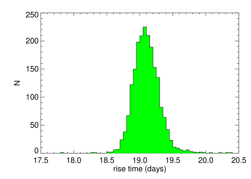
Figure 1: Rise-time ($\tau_{r}$) histogram for 73 SNLS SNe Ia, taking into account the correlations between data points as described in §2. This represents 2000 realizations of the light curve parameters. The mean value is 19.10 days.

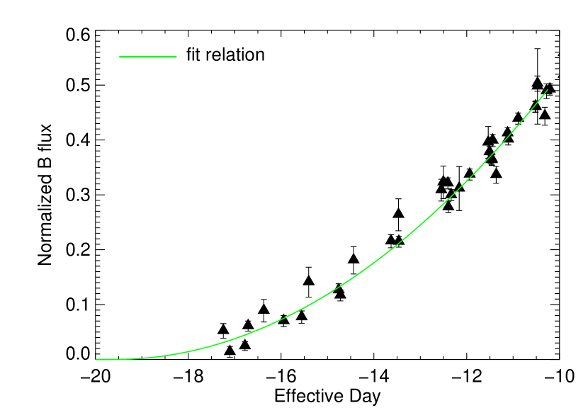
Figure 2: Data in the rise-time region for the eight nearby SNe Ia used in this study. These have been combined using the techniques described in §2.

It is also quite interesting to compare the rise-time measurements for different subsamples of our data. The results of these fits are given in table 2. We do not consider these subsets of the nearby sample because it is too small. First, we consider splitting by redshift to search for evolution within our sample. The median redshift is 0.647. This is quite close to the transition between observer frame $r^{\prime}$ matching with rest-frame $B$ and $i^{\prime}\mapsto B$, which takes place at $z=0.589$. This test is therefore sensitive to two possible effects: evolution, and a calibration mismatch between $r^{\prime}$ and $i^{\prime}$. Because we cannot test each of these independently, we split at $z=0.589$, which results in 29 SNe Ia in the intermediate-$z$ sample and 44 in the high-$z$ sample ($\left<z\right>=0.43$ and $0.74$, respectively). The photometric noise in the high-$z$ portion of the sample is much larger than in the intermediate-$z$ portion, as shown in figure 3. This figure also demonstrates that data from different SNe Ia can be combined quite accurately using the techniques described in §2.

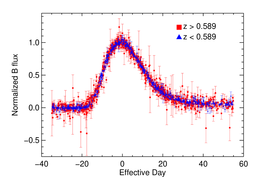
Figure 3: Shifted, normalized, and $K$-corrected SNLS data split by redshift and over-plotted. The rest-frame $B$ band is shown. Observations in the same filter on the same night are combined for display purposes; the actual fit is performed on the individual data points. The blue triangles represent redshifts where rest-frame $B$ matches the $r^{\prime}$ filter, and the red squares where $i^{\prime}$ is the best match.

The data in the rise-time region are shown in figure 4, again split into the two groups. Using the same analysis, for $z\leq 0.589$ we measure $\tau_{r}=19.01^{+0.19}_{-0.18}$ days and for $z>0.589$ we measure $\tau_{r}=19.67^{+0.54}_{-0.49}$ days. The intermediate-$z$ portion of the sample clearly dominates the fit to the full sample. These are statistically compatible (the difference is 1.2 $\sigma$).

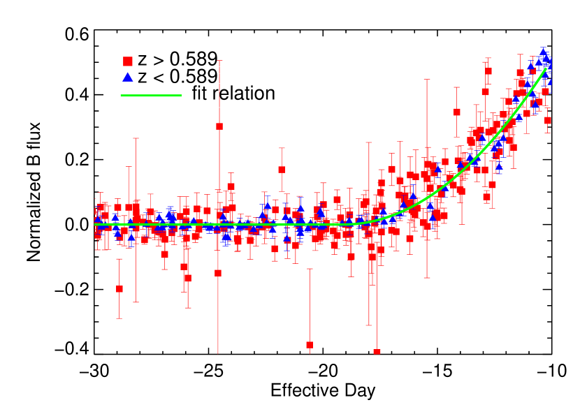
Figure 4: Data in the rise-time region for the 73 SNLS SNe Ia used in this study, combined using the techniques described in §2. They are split by redshift as in figure 3. Observations from the same filter on the same night have been combined for display purposes.

As a test of whether the stretch model works at such early times, we split the sample by stretch. Unlike the nearby sample, one cannot measure the rise time precisely for most of the distant SNe Ia individually, so this test must be done on a sample-wide basis. Splitting around the mean stretch, the low-stretch sample ($s\leq 0.99,\left<s\right>=0.92$) of 36 SNe gives $\tau_{r}=19.20^{+0.33}_{-0.34}$ days and the high-stretch sample ($s>0.99,\left<s\right>=1.05$, 37 SNe) gives $\tau_{r}=19.09^{+0.33}_{-0.20}$ days. These straddle the full sample value, and are statistically indistinguishable (0.3 $\sigma$ difference). If stretch did not work at early times, we generally would not expect these to agree.

We can also split the sample by host galaxy star formation rate, following the methodology of Sullivan et al. (2006). Briefly, the broadband colors of the host galaxies are fitted by a galaxy spectral evolution code using the known redshift to determine the star formation rate per unit mass (sSFR), measured in yr^-1. The sample is then split between SNe in hosts with no star formation (passive, zero sSFR), those with moderate star formation rates (active, $-12\leq\log_{10}{sSFR}\leq-9.5$), and those with a large amount of star formation (vigorously star forming, $\log_{10}{sSFR}>-9.5$). We follow the above paper in limiting the application of this technique to $z\leq 0.75$, where it is most reliable for our data set. This results in a sample of 9 SNe Ia in passive hosts, 11 in active galaxies, and 35 in vigorously star forming galaxies. Clearly, this is an area where an increased sample size would be beneficial. Note that the comparison of these subsets is not independent of the stretch comparison: there is a relation between stretch and host galaxy morphology (Hamuy et al., 2000) and, in addition, star-formation rate (Gallagher et al., 2005) for nearby SNe Ia that has recently been confirmed at high redshift in the SNLS sample (Sullivan et al., 2006). In any case, for the passive sample we find a value of $\tau_{r}=20.40^{+1.04}_{-1.10}$ days, for the active sample $\tau_{r}=18.95^{+0.40}_{-0.41}$ days, and for the vigorously star-forming sample $\tau_{r}=19.07^{+0.19}_{-0.18}$ days. The rise time in passive hosts is mildly different than the others but only at the 1.2 $\sigma$ level. The data is shown in figure 5.

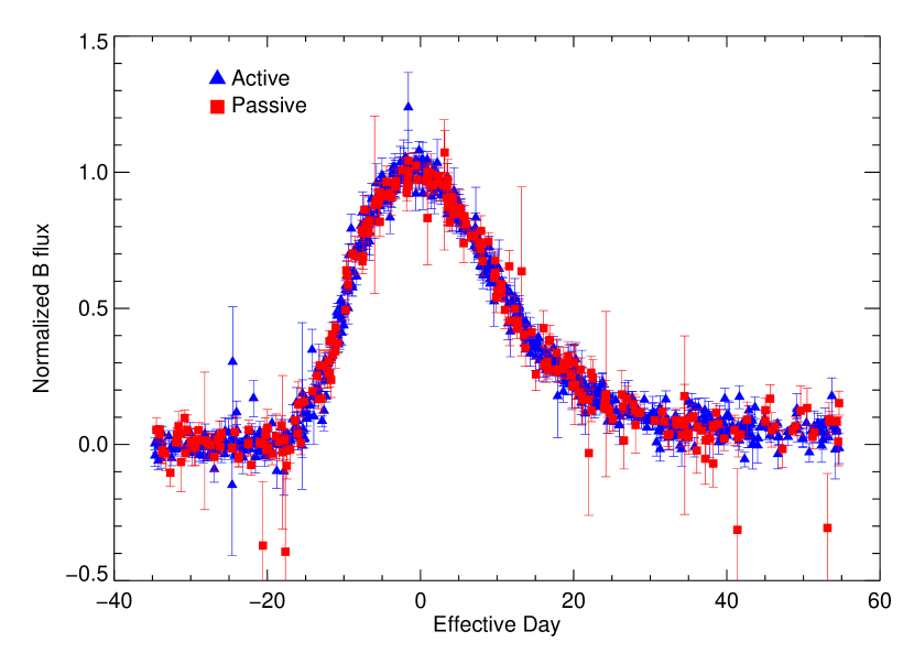
Figure 5: Shifted, normalized, and $K$-corrected SNLS data split by host galaxy specific star formation rate. In all other respects this is identical to figure 3. The blue triangles include SN from both active and vigorously star forming hosts as defined in §5 ($\log_{10}{sSFR}>-12$), while the red squares show those from from passive hosts.

Table 2: Results of rise-time fits

fit	$N_{\mbox{SN}}$	$\tau_{r}$ (days)	Notes
SNLS	73	$19.10^{+0.18\ 0.42}_{-0.17\ 0.36}$	$\cdots$
nearby	8	$19.58^{+0.22\ 0.46}_{-0.19\ 0.38}$	$\cdots$
SNLS intermediate $z$	29	$19.01^{+0.18\ 0.37}_{-0.18\ 0.36}$	$z\leq 0.589$, $\left<z\right>=0.43$
SNLS high $z$	44	$19.67^{+0.54\ 1.13}_{-0.49\ 0.99}$	$z>0.589$, $\left<z\right>=0.74$
SNLS low $s$	36	$19.20^{+0.33\ 0.67}_{-0.34\ 0.67}$	$s\leq 0.99$, $\left<s\right>=0.92$
SNLS high $s$	37	$19.09^{+0.20\ 0.39}_{-0.20\ 0.40}$	$s>0.99$, $\left<s\right>=1.05$
SNLS passive hosts	9	$20.40^{+1.04\ 1.73}_{-1.10\ 2.06}$	$\log_{10}{sSFR}<-12.0$
SNLS active hosts	11	$18.95^{+0.40\ 0.74}_{-0.41\ 0.83}$	$-12\leq\log_{10}{sSFR}\leq-9.5$
SNLS vigorous hosts	35	$19.07^{+0.19\ 0.40}_{-0.18\ 0.37}$	$\log_{10}{sSFR}>-9.5$

Note. — Rise-time fits to various samples. sSFR is the star formation rate per unit mass in units of $\mbox{yr}^{-1}$.

The dominant systematic error for our measurement should arise from the $K$-corrections. Given the relative rarity of early-time photometry of nearby SNe Ia at early epochs, it is not surprising that there is very little spectroscopy available in the rise-time region. Hence, our ability to combine data from SNe Ia at different redshifts accurately is highly dependent on the theoretical models used to derive the SED at these epochs. At sufficiently early times SNe Ia should have SEDs dominated by thermal continuum. However, it is not observationally clear at what point this becomes a poor approximation.

We have tried to quantify this by considering the effects of using a different, largely independently derived set of spectral templates, specifically those of Nobili et al. (2003). Redoing the above analysis, including the light-curve fits, shifts the rise time by 0.2 days. We take this as an estimate of the systematic uncertainty arising from $K$-corrections. AKN00 also considered the effects of changing the late-time light-curve behavior, arguing that this gave an upper limit for the systematic error of 2–3 days. However, the conditions considered were somewhat extreme, namely that all of the high-redshift sample have unusual late-time behavior when compared with the nearby sample. As an upper limit this is reasonable, but as a systematic estimate it is quite conservative. We expect that the systematic error involved in comparing different subsets of the SNLS sample against each other should be smaller, since uncertainties in the SED should affect the two samples in a similar fashion. In any case, since the subset comparisons reveal no effect even without systematic errors, we have not tried to estimate them.

Ideally for the low-redshift sample $K$-corrections should not be a problem. The SNe Ia in the current nearby rise-time sample are all essentially at zero redshift, and so if the observations were on the standard photometric system there would essentially be no SED dependence of this process. Unfortunately this is not the case; a significant portion of the nearby data comes from unfiltered observations. We are not in a position to use the same technique to estimate the systematic error on the nearby data. R99 discussed some of the uncertainties associated with transforming to the standard pass bands, but choose to include these effects as large statistical errors rather than as an overall systematic effect. Therefore, we simply have to trust that our derived statistical errors incorporate systematic uncertainties due to $K$-corrections for the nearby sample.

6 CONCLUSIONS

We have measured the rise time from a sample of 73 high redshift ($z=0.15-0.9$) spectroscopically confirmed SNe Ia discovered and observed by the SNLS. This determination is roughly 6 times more precise than those previously available in this redshift range (AKN00, G01). Our measurement for this sample is $\tau_{r}=19.10^{+0.18}_{-0.17}\left(\mbox{stat}\right)\pm 0.2\left(\mbox{syst}\right)$ days. Using the same analysis technique on a sample of eight nearby SNe Ia ($z<0.1$), we derive a value of $\tau_{r}=19.58^{+0.22}_{-0.19}$ days, where the quoted error incorporates both statistical and systematic errors. These differ at the 1.4 $\sigma$ level. In other words, using a considerably more precise comparison made possible by a substantially better data set, we find no compelling evidence for any difference between the rise times of nearby and distant SNe Ia. It is important to understand the limitations of this measurement in terms of its constraints on theoretical models. As was the case in R99, AKN00, and G01, the uncertainties presented above are the error in the mean stretch-corrected rise times of the two samples, not the scatter of rise times between individual SNe Ia. However, testing for differences between the two samples is still a very useful check against evolutionary effects that may be affecting cosmological analyses using SNe Ia.

The above result suggests that we are currently limited by the systematic uncertainty associated with $K$-corrections in performing this comparison. Therefore, significant advances will likely require better constraints on the early-time SEDs of SNe Ia. Alternatively, for a large enough sample, it may be possible to constrain the rise-time by only considering redshifts for which the observer and rest-frame filters match particularly well, minimizing the $K$-correction errors.

The quadratic rise-time model, motivated by simple physical arguments, provides a good fit to the data. Dropping this assumption, we find $n=1.8\pm 0.2$ for $f\propto t^{n}$ at early times. Fitting for this extra parameter substantially weakens our constraints on $\tau_{r}$, but does not indicate any discrepancies. Redoing the fits with $n$ fixed at this value also does not significantly affect any of our results, simply decreasing all of the measurements of $\tau_{r}$ by $\sim 0.6$ days.

We have also split the SNLS sample into subsets and searched for differences between them. The comparisons we consider are splitting the sample by redshift at $z=0.589$ to test for evolution within our sample and for calibration systematics, splitting by stretch, and splitting by host galaxy star formation rate. In all of these cases the subsamples give compatible rise times. The fact that the low- and high-stretch samples agree confirms the claim of G01 that the stretch parameterization works both at early and late times, at least up until around day 35. Unlike the rise-time fit to the full sample, for many of these subsets we are limited by statistics, so as the survey continues more sensitive comparisons will be possible. Once a full cosmological analysis on all these SN is available, it will also be interesting to check whether there is any correlation between the residual from the best fitting cosmology and rise time.

References

- Aldering et al. (2000) Aldering, G., Knop, R., and Nugent, P. 2000, AJ 119, 2110, astro-ph/0001049
- Astier et al. (2006) Astier, P., et al. 2006, A&A 447, 31, astro-ph/0510447
- Benetti et al. (2004) Benetti, S., et al. 2004, MNRAS 348, 261, astro-ph/0309665
- Blondin et al. (2006) Blondin, S., et al. 2006, AJ 131, 1648, astro-ph/0510089
- Boulande et al. (2003) Boulande, O., et al. in Instrument Design and Performance for Optical/Infrared Ground-based Telescopes, ed. Iye, Masanori, Moorwood, Alan F.M., Proc. SPIE 4841, 72
- Branch (1992) Branch, D. 1992, ApJ 392, 35
- Contardo et al. (2000) Contardo, G., Leibundgut, B. and Vacca, W.D. 2000, A&A 359, 876, astro-ph/0005507
- Domínguez et al. (2001) Domínguez, I., Höflich, P., and Straniero, O. 2001, ApJ 2001, 557, 279, astro-ph/0104257
- Gallagher et al. (2005) Gallager, J.S., et al. 2005, ApJ 634, 210, astro-ph/0508180
- Goldhaber et al. (2001) Goldhaber, G., et al. 2001, ApJ 558, 359, astro-ph/0104382
- Guy et al. (2005) Guy, J., et al. 2005, A&A 443, 781, astro-ph/0506583
- Hamuy et al. (2000) Hamuy, M., et al. 2000, AJ 120, 1479, astro-ph/0005213
- Höflich et al. (1993) Höflich, P., Müeller, E., and Khokhlov, A. 1993, A&A 268, 570
- Höflich & Khokhlov (1996) Höflich, P. and Khokhlov, A. 1996, ApJ 457, 500, astro-ph/9602025
- Höflich et al. (1998) Höflich, P., Wheeler, J.C., and Thielemann, F.K. 1998, ApJ 495, 617, astro-ph/9709233
- Höflich et al. (2002) Höflich, P., et al. 2002, ApJ 568, 791, astro-ph/0112126
- Hook et al. (2005) Hook, I.M., Howell, D.A., et al. 2005, AJ, 130, 2788, astro-ph/0509041
- Howell et al. (2005) Howell, D.A., et al. 2005, ApJ 634, 1190, astro-ph/0509195
- James & Roos (1975) James, F. and Roos, M. 1975, Compt. Phys. Comm. 10, 343
- Jha et al. (2006) Jha, S., et al. 2006, AJ 131, 527, astro-ph/0509234
- Khokhlov et al. (1993) Khokhlov, A., Mueller, E., and Höeflich, P. 1993, A&A 270, 233
- Knop et al. (2003) Knop, R.A., et al. 2003, ApJ 598, 102, astro-ph/0309368
- Krisciunas et al. (2003) Krisciunas, K., et al. 2003, AJ 125, 166, astro-ph/0210327
- Krisciunas et al. (2004) Krisciunas, K., et al. 2004, AJ 128, 3034, astro-ph/0409036
- Lira et al. (1998) Lira, P., et al. 1998, AJ 115, 234, astro-ph/9709262
- Nobili et al. (2003) Nobili, S., et al. 2003, A&A 404, 901, astro-ph/0304240
- Nugent et al. (2002) Nugent, P., Kim, A., and Perlmutter, S. 2003, PASP 114, 803, astro-ph/0205351
- Perlmutter et al. (1999) Perlmutter, S., et al. 1999, ApJ 517, 565, astro-ph/9812133
- Pskovskii (1984) Pskovskii, Yu.P., 1984, Soviet Ast. 28, 658
- Richmond et al. (1995) Richmond, M.W., et al. 1995, AJ 109, 2121
- Riess et al. (1996) Riess, A.G., et al. 1996, ApJ 473, 88, astro-ph/9604143
- Riess et al. (1998) Riess, A.G., et al. 1998, AJ 116, 1009, astro-ph/9805201
- Riess et al. (1999a) Riess, A.G., et al. 1999, AJ 118, 2675, astro-ph/9907037
- Riess et al. (1999b) Riess, A.G., Filippenko, A.V., Li., W, and Schmidt, B.P. 1999, AJ 118, 2668, astro-ph/9907038
- Riess et al. (2005) Riess, A.G., et al. 2005, ApJ 627, 579, astro-ph/0503159
- Shigeyama et al. (1992) Shigeyama, T., Nomoto, K., Yamaoka, H., and Theilemann, F.K. 1992, ApJ 386, 13
- Sullivan et al. (2003) Sullivan, M., et al. 2003, MNRAS 340, 1057, astro-ph/0211444
- Sullivan et al. (2006) Sullivan, M., et al. 2006, ApJ, in press, astro-ph/0605455
- Vacca & Leibundgut (1996) Vacca, W.D., and Leibundgut, B. 1996, ApJ 471, L37, astro-ph/9608181