Scale-Free Thin Discs with an Isopedic Magnetic Field

Abstract

Global stationary configurations of both aligned and logarithmic spiral magnetohydrodynamic (MHD) perturbations are constructed analytically within an axisymmetric background of razor-thin scale-free gas disc, which is embedded in an axisymmetric gravitational potential of a dark matter halo and involves an isopedic magnetic field almost vertically threaded through the disc plane. The scale-free index $\beta$ of the disc rotation speed $v_{\theta}\propto R^{-\beta}$ falls in the range of $(-1/2\ ,\ 1/2)$ where $R$ is the cylindrical radius. With the holding-back of a deep background dark matter halo potential, the isopedic magnetic field may be strong enough to allow for the magnetic tension force overtaking the disc self-gravity, which can significantly influence global stationary MHD perturbation configurations and stability properties of the scale-free disc system. Only for stationary logarithmic spiral MHD perturbations with a perturbation scale-free index $\beta_{1}=1/4$ or for aligned stationary MHD perturbations, can the MHD disc maintain a constant radial flux of angular momentum. The variable radial flux of angular momentum in the radial direction corresponds to a complex dispersion relation. The marginal instabilities for axisymmetric MHD disturbances are also examined for a special case as an example. When the magnetic tension force overtakes the disc self-gravity, the scale-free disc can be completely stable against axisymmetric MHD disturbances of all wavelengths. We predict the possible existence of an isopedically magnetized gas disc system in rotation primarily confined by a massive dark matter halo potential.

1 Introduction

As an important intermediate stage of many astrophysical processes, the dynamics of magnetized disc systems are frequently invoked to model different phenomena on various spatial and temporal scales, such as spiral or barred-spiral galaxies, magnetized accretion discs surrounding supermassive black holes (SMBHs) anchored at galactic centres, accreting environs involving binary stars and protoplanetary systems etc. It is therefore of considerable interest to study magnetohydrodynamic (MHD) processes in discs for both theoretical and applied purposes. The pioneer development of the classic density wave theory for large-scale perturbation structures in differentially rotating discs (Lin & Shu 1964, 1966) has opened up a physical scenario to understand the basic dynamics of spiral galaxies (Lin 1987; Binney & Tremaine 1987; Bertin & Lin 1996). Linear perturbation or nonlinear theories are widely used as powerful tools of analysis to explore the structure and stability of disc systems. In many processes, initially small perturbations may lead to more violent consequences (e.g., gravitational collapse of a central core) which are crucial for the dynamical evolution of astrophysical systems. In various contexts, MHD perturbation configurations are valuable indicators of transitions to instabilities and of further dynamical structure and evolution.

For simplicity and clarity, the scale-free disc system as an idealized model is a frequent target of theoretical investigation. The concept of a ‘scale-free’ or a ‘self-similar’ disc means all relevant physical quantities in the disc system vary as powers of cylindrical radius $R$ such that the disc system carries no characteristic length scale (e.g., the linear speed of disc rotation $v_{\theta}\propto R^{-\beta}$ and the equilibrium disc surface mass density $\Sigma_{0}\propto R^{-2\beta-1}$ etc. with $\beta$ being a constant exponent). Given possible situations, one may introduce ‘boundary conditions’ to describe a modified scale-free disc by cutting a central hole in a disc (e.g., Zang 1976; Evans & Read 1998a, b) or by limiting the radial extent of a disc. Observationally, many disc galaxies show more or less flat rotation curves, indicating the presence of massive dark matter halos according to the Newtonian gravity theory. Theoretically, discs with flat rotation curves (i.e., the azimuthal velocity $v_{\theta}=\mbox{const}$ or $\beta=0$) belong to a specific subclass of scale-free discs, referred to as singular isothermal discs (SIDs). Since the seminal analysis of Mestel (1963), the SID model has attracted considerable attention in various astrophysical contexts (e.g., Zang 1976; Toomre 1977; Lemos, Kalnajs & Lynden-Bell 1991; Shu et al. 2000; Lou 2002; Lou & Fan 2002; Lou & Shen 2003; Shen & Lou 2004a,b; Lou & Zou 2004, 2006; Shen, Liu & Lou; Lou & Wu 2005; Lou & Bai 2006). In most normal spiral galaxies, disc rotation curves tend to be flat over extended radii, giving a strong evidence for the existence of massive dark matter halos (e.g., Rubin et al. 1982; Kent 1986, 1987, 1988). Given the inferred dominant masses, we recognize that a dark matter halo plays extremely important roles in the dynamical evolution of a disc galaxy (Miller et al. 1970; Ostriker & Peebles 1973; Hohl 1971; Miller 1978; Binney & Tremaine 1987).

Besides the normal mode perturbation analysis in scale-free discs (e.g., Zang 1976; Binney & Tremaine 1987; Fan & Lou 1997; Evans & Read 1998a,b; Goodman & Evans 1999; Shu et al. 2000), the zero-frequency neutral perturbation modes or stationary perturbation configurations are emphasized as the marginal instability in scale-free discs (e.g., Lemos et al. 1991; Syer & Tremaine 1996; Shu et al. 2000; Lou & Shen 2003; Shen & Lou 2003; Shen & Lou 2004a; Shen et al. 2005; Lou & Zou 2004, 2006; Lou & Wu, 2005; Lou & Bai 2006). Axisymmetric instabilities are thought to set in through transitions across such neutral modes (Safronov 1960; Toomre 1964; Lynden-Bell & Ostriker 1967; Lemos et al. 1991; Shu et al. 2000). Parallel to zero-frequency modes for axisymmetric disturbances, Shu et al. (2000) tentatively proposed that logarithmic spiral modes of stationary perturbation configurations also signal onsets of non-axisymmetric instabilities; the resulting criterion appears to be compatible with the criterion of Goodman & Evans (1999) for instabilities in their normal mode approach. Recently, Shen & Lou (2004a) extended the analysis of Shu et al. (2000) in a gravitationally coupled composite scale-free disc system of gaseous and stellar discs using a two-fluid formalism. In solving nonlinear MHD equations, it is a challenge to achieve analytical results unless some simplified assumptions are introduced, such as the stationarity ($\omega=0$) condition etc. Most results are analytic in this paper and it is highly desirable that numerical simulations should be developed as touchstones for the analytical results and further venture into new regimes where analytical methods cannot reach (Syer & Tremaine 1996).

Magnetic field receives considerable attention in astrophysics, and contributes to structures, dynamics and diagnostics on various scales of different astrophysical systems (Sofue et al. 1986; Beck et al. 1996; Balbus & Hawley 1998; Kaburaki 2000, 2001; Balbus 2003; Vallée 2004; Hu & Lou 2004; Yu & Lou 2006; Yu, Lou, Bian & Wu 2006). Prompted by numerical simulations of magnetized cloud core formation through the ambipolar diffusion (e.g., Nakano 1979; Lizano & Shu 1989), Shu & Li (1997) introduced the so-called ‘isopedic’ condition requiring that the $z-$component flux ($B_{z}$ in cylindrical coordinates) of an open magnetic field, which threads through the disc almost vertically, is proportional to the disc surface mass density ($\Sigma$) or $B_{z}/\Sigma=\mbox{const}$. With this simple and justifiable assumption (Lou & Wu 2005), effects of such an isopedic magnetic field can be simply subsumed into relevant terms in MHD equations (Shu & Li 1997); this simplification is powerful in analytical analysis in comparison with the usual awesome MHD equations describing the roles of magnetic field. Lou & Wu (2005) discussed the global MHD perturbation configurations in a composite SID system of coupled gas and stellar components with an isopedic (vertical) magnetic field. Lou & Zou (2004, 2006) investigated the similar kind of composite MHD SID problems except that their magnetic field is coplanar rather than isopedic. Lou & Bai (2006) analyzed MHD perturbation structures in a composite system of two coupled scale-free discs with a coplanar magnetic field.

The purpose of this paper is to couple an isopedic magnetic field with a single scale-free gas disc embedded in an axisymmetric dark matter halo potential and to construct physically allowed global stationary MHD perturbation configurations in such a disc as well as to investigate the instability of such a disc system. Parallel to the hydrodynamic treatment of Syer & Tremaine (1996), our analysis leads to further MHD extensions and generalizations. To be specific, six components of forces are involved in the disc equilibrium of our analysis, namely, the radial centrifugal force, the thermal gas pressure force in the disc, the self-gravity of the disc, the holding-back gravity force of an axisymmetric dark matter halo and the tension and pressure forces resulting from an isopedic magnetic field within the disc plane. While highly idealized, the unique combination of these essential elements of a disc galaxy does provide a new perspective and has already shown some novel characteristics. For example, the introduction of an isopedic magnetic field geometry in a scale-free disc does bring several new and interesting features in reference to prior related disc model analyses (Syer & Tremaine 1996; Shu et al. 2002; Shen & Lou 2004b; Lou & Zou 2004, 2006; Shen, Liu & Lou 2005; Lou & Wu 2005; Lou & Bai 2006).

This paper is organized as follows. In Section 2, we describe the basic MHD model of a scale-free razor-thin disc. In Section 3, isopedic magnetic field are discussed under the scale-free condition. In Section 4, we construct the stationary background axisymmetric equilibrium in a rotational MHD balance. In Section 5, a generalized MHD dispersion relationship is derived for MHD perturbations. We investigate the global stationary aligned MHD cases in Section 6 and stationary unaligned MHD (logarithmic spiral) cases in Section 7. We summarize the results and provide discussions in Section 8. Specific details of derivations are contained in Appendices.

2 A Class of Scale-Free Razor-Thin Discs

Formally, a razor-thin disc has a three-dimensional mass density mathematically described by

$$\rho(R,\ \theta,\ z,\ t)=\Sigma(R,\ \theta,\ t)\delta(z)\ ,$$ (1)

where cylindrical coordinates $(R,\theta,z)$ are adopted, $\Sigma(R,\theta,t)$ is the two-dimensional surface mass density and $\delta(z)$ is the Dirac $\delta$-function with the vertical coordinate $z$ as the argument. Except for the three-dimensional gravitational potential, any physical quantity $q$ is a function of $R$, $\theta$ and $t$ as $q(R,\theta,\ t)$ for a razor-thin disc.

In a razor-thin disc, the vertically integrated barotropic equation of state has a ‘two-dimensional’ form of

$$\Pi=k\Sigma^{\Gamma}\ ,$$ (2)

where $\Pi(R,\theta,t)$ represents the two-dimensional gas pressure, constant coefficient $k\geq 0$ and the barotropic index $\Gamma>0$. We here take the general ‘three-dimensional’ polytropic equation of state $p=\tilde{k}\rho^{\gamma}$ for a comparison

$$\qquad\qquad\Pi(R,\ \theta,\ t)\equiv\int_{\Delta z}p(R,\ \theta,\ z,\ t)\mathrm{d}z\ \qquad\leftrightarrow\ \qquad\Sigma(R,\ \theta,\ t)\equiv\int_{\Delta z}\rho(R,\ \theta,\ z,\ t)\mathrm{d}z\ ,$$

where $\Pi$ is determined by vertically integrating the thermal gas pressure $p$. Given certain assumptions such as $\Pi\propto\Sigma p_{c}/\rho_{c}$ with $p_{c}$ and $\rho_{c}$ being the central pressure and density, a relationship between the two indices $\Gamma$ and $\gamma$ can be established as $\Gamma=3-2/\gamma$ (see equation 3.5 of Lemos et al. 1991).

The sound speed $v_{s}$ in a barotropic disc can be defined as

$$v_{s}^{2}\equiv\frac{\mathrm{d}\Pi}{\mathrm{d}\Sigma}=k\Gamma\Sigma^{\Gamma-1}=\Gamma\Pi/\Sigma$$ (3)

and the enthalpy $H$ is expressed by

$$H=\int\frac{\mathrm{d}\Pi}{\Sigma}=\frac{k\Gamma\Sigma^{\Gamma-1}}{(\Gamma-1)}\ .$$ (4)

The gravitational potential $\Phi(R,\ \theta,\ t)$ in the disc plane and the disc surface mass density is related by the Poisson integral

$$\Phi(R,\ \theta,\ t)=\int\int\frac{-G\Sigma(r,\ \phi,\ t)r\mathrm{d}r\mathrm{d}\phi}{[r^{2}+R^{2}-2Rr\cos(\theta-\phi)]^{1/2}}\ ,$$ (5)

where $G$ is the gravitational constant.

Among various model problems in disc dynamics, the scale-free disc model is often picked up by theorists for its relative simplicity and is explored as a powerful vehicle for a global analytical analysis. Scale-free discs carry no characteristic spatial scales. For a mathematical approach to scale-free discs, we adopt the definition given by Lynden-Bell & Lemos (1999). A flat disc is scale-free if any physical quantity $q(R,\ \theta)$ of a disc configuration has the following relationship

$$q\left(\zeta R,\ \theta+h(\zeta)\right)=A_{1}(\zeta)q(R,\ \theta)\ ,$$ (6)

where $\zeta$ is a parameter, and $h(\zeta)$ and $A_{1}(\zeta)$ are two arbitrary functions. By requirement (6), $q$ has a general solution form of

$$q=R^{\alpha}F(\theta+\mu\ln R)\ ,$$ (7)

where $\alpha$ is complex, $\mu$ is real, and $F$ is an arbitrary function. The proof can be found in Lynden-Bell & Lemos (1999).

Fluid equations provide a valid dynamical description for a gas disc component, while distribution function equations are more appropriate for a collisionless stellar disc component (e.g., Binney & Tremaine 1987). After an introduction of the velocity dispersion of the stellar disc component regarded as an effective ‘sound speed’, fluid equations can be approximately applied to stellar disc component as well (Lin & Shu 1964, 1966; Lin 1987; Binney & Tremaine 1987; Bertin & Lin 1996; Lou & Shen 2003; Shen & Lou 2004a; Lou & Zou 2004, 2006; Lou & Wu 2005; Lou & Bai 2006).

In treating a razor-thin scale-free disc system, we adopt two-dimensional fluid equations. The three basic fluid equations of describing razor-thin disc dynamics can be written as

$$\frac{\partial\Sigma}{\partial t}+\frac{1}{R}\frac{\partial}{\partial R}(R\Sigma v_{R})+\frac{1}{R}\frac{\partial}{\partial\theta}(\Sigma v_{\theta})=0\ ,$$ (8)

$$\frac{\partial v_{R}}{\partial t}+v_{R}\frac{\partial v_{R}}{\partial R}+\frac{v_{\theta}}{R}\frac{\partial v_{R}}{\partial\theta}-\frac{v_{\theta}^{2}}{R}=-\frac{1}{\Sigma}\frac{\partial\Pi}{\partial R}-\frac{\partial(\Phi+\bar{\Phi})}{\partial R}=-\frac{\partial(H+\Phi+\bar{\Phi})}{\partial R}\ ,$$ (9)

$$\frac{\partial v_{\theta}}{\partial t}+v_{R}\frac{\partial v_{\theta}}{\partial R}+\frac{v_{\theta}}{R}\frac{\partial v_{\theta}}{\partial\theta}+\frac{v_{\theta}v_{R}}{R}=-\frac{1}{\Sigma R}\frac{\partial\Pi}{\partial\theta}-\frac{\partial(\Phi+\bar{\Phi})}{R\partial\theta}=-\frac{\partial(H+\Phi+\bar{\Phi})}{R\partial\theta}\ ,$$ (10)

where $v_{R}$ is the radial bulk flow velocity and $v_{\theta}$ is the azimuthal bulk flow velocity and $\bar{\Phi}$ represents the axisymmetric background halo potential presumed to be unperturbed, i.e., $\bar{P}$ parameter remains unchanged in equation (11). The last equalities in equations (9) and (10) corresponds to the barotropic condition.

In order to meet the scale-free requirement (Syer & Tremaine 1996; Goodman & Evans 1999; Shen & Lou 2004a; Shen, Liu & Lou 2005), we presume relevant physical quantities in the following forms of

$$\qquad\qquad\Sigma=R^{-2\beta-1}S(\varphi)\ ,\quad\qquad v_{R}=R^{-\beta}a(\varphi)\ ,\quad\qquad v_{\theta}=R^{-\beta}b(\varphi)\ ,$$

$$\qquad\qquad\Phi=-R^{-2\beta}P(\varphi)\ ,\quad\qquad\bar{\Phi}=-R^{-2\beta}\bar{P}\ ,\quad\qquad H=R^{-2\beta}Q(\varphi)\ ,$$ (11)

where we define $\varphi(R,\ \theta)\equiv\theta+\mu\ln R$ and $\beta$ is a scale-free index. Both $\mu$ and $\beta$ are constant real coefficients here.

To satisfy the scale-free condition in equation (4), we should require

$$(-2\beta-1)(\Gamma-1)=-2\beta\quad\Rightarrow\quad\Gamma=(1+4\beta)/(1+2\beta)\ .$$ (12)

The constraint $\Gamma>0$ for a warm disc ($k>0$) implies either $\beta>-1/4$ or $\beta<-1/2$ and thus ensures $v_{s}^{2}>0$. For a cold disc ($k=0$), such a constraint is unnecessary.

Other constraints on $\beta$ come from the disc mass distribution. First, $\Sigma$ is assumed to decrease with increasing $R$ and this implies $\beta>-1/2$ by the first relation in equation (11). Secondly, the central mass should be finite. This simply means

$$\qquad\qquad\lim_{r\rightarrow 0}\int_{0}^{r}\int_{0}^{2\pi}\Sigma(R,\theta)R\mathrm{d}R\mathrm{d}\theta=\lim_{r\rightarrow 0}\int_{0}^{r}\int_{0}^{2\pi}R^{-2\beta}S(\theta+\mu\ln R)\mathrm{d}R\mathrm{d}\theta=\int_{0}^{2\pi}S(\theta)\mathrm{d}\theta\lim_{r\rightarrow 0}\left.\frac{R^{1-2\beta}}{1-2\beta}\right|_{0}^{r}<+\infty\ .$$

We then require $1-2\beta>0$, indicating $\beta<1/2$. In short, we therefore have $-1/2<\beta<1/2$ based on the requirement of the disc mass distribution.

Moreover, the allowed range of $\beta$ is constrained by the convergence of the Poisson integral relating $\Sigma$ and $\Phi$. According to the analytical results of Qian (1992), for $\Sigma(R,\theta)=R^{-2\beta-1+\mathrm{i}\nu}\exp({\mathrm{i}m\theta})=R^{-2\beta-1}\exp[{\mathrm{i}(m\theta+\nu\ln R)}]$ with $\nu$ being a real constant parameter, we have correspondingly

$$\Phi(R,\theta)=-GY_{m}\left(\beta-\mathrm{i}\nu/2\right)R^{-2\beta+\mathrm{i}\nu}\exp({\mathrm{i}m\theta})\ ,$$ (13)

where $Y_{m}(x)$ is defined in terms of the standard $\Gamma$ function as

$$Y_{m}(x)\equiv\frac{\pi\displaystyle\Gamma({m}/{2}-x+{1}/{2})\Gamma({m}/{2}+x)}{\displaystyle\Gamma({m}/{2}-x+1)\Gamma({m}/{2}+x+{1}/{2})}\ .$$ (14)

The above expression remains valid only for $-m/2<\beta<(m+1)/2$; outside this range of $\beta$, the force from gas materials at either $r\rightarrow\infty$ or $r\rightarrow 0$ diverges (Qian 1992). When $m\geq 1$, potential expression (13) remains valid for $\beta\in(-1/2,\ 1/2)$. For the $m=0$ case, although the potential $\Phi$ in equation (13) converges only for $\beta\in(0,\ 1/2)$, we can extend the valid range to $\beta\in(-1/2,1/2)$ if we only make use of $\nabla\Phi$ to compute the force, which suffices for our purpose (Syer & Tremaine 1996).

We frequently refer to the Kalnajs function (Kalnajs 1971; Shu et al. 2000) which is explicitly defined by

$${\mathcal{N}}_{m}(\nu)\equiv K(\nu,m)=\frac{1}{2}\frac{\Gamma[(m+1/2+\mathrm{i}\nu)/2]\Gamma[(m+1/2-\mathrm{i}\nu)/2]}{\Gamma[(m+3/2+\mathrm{i}\nu)/2]\Gamma[(m+3/2-\mathrm{i}\nu)/2]}=\frac{Y_{m}\left({1}/{4}-\mathrm{i}\nu/2\right)}{2\pi}\ .$$ (15)

For $m\neq 0$ and setting $\mu\equiv\nu/m$, we write $\exp[{\mathrm{i}(m\theta+\nu\ln R)}]=\exp({\mathrm{i}m\varphi})$. For $m=0$, expression $\exp({\mathrm{i}\nu\ln R})$ should replace expression $\exp({\mathrm{i}m\varphi})$ in treating axisymmetric perturbations (Syer & Tremaine 1996). We write perturbations in the form of $\exp[{\mathrm{i}(m\theta+\nu\ln R)}]$ instead of $\exp({\mathrm{i}m\varphi})$ throughout our analysis unless otherwise stated.

We note that from the scale-free condition (Lynden-Bell & Lemos 1999), there is no a priori reason that the scale-free index $\alpha$ (see equation 7) should be necessarily real. However, the imaginary part $\Im(\alpha)$ will make such term as $\exp[{\mathrm{i}\Im(\alpha)\ln R}]$ oscillating around 0. For example, the surface mass density $\Sigma=R^{\alpha}$ could be negative when $\Im(\alpha)\neq 0$. From the physical perspective, only a perturbation term may have such non-zero imaginary part of the scale-free index $\alpha$.

Finally, we conclude that the gravitational potential of a scale-free disc is given by expression (13) and the constraint for scale-free index $\beta$ is $\beta\in(-1/2,\ 1/2)$ for cold discs (i.e., $k=0$) and $\beta\in(-1/4,\ 1/2)$ for warm discs (i.e., $k>0$).

3 An Isopedic Magnetic Field across a Scale-Free Thin Disc

The generation, amplification, and activities of magnetic field are widely believed to be caused by nonlinear MHD dynamo processes in an electrically conducting gas medium (e.g., Parker 1979; Moffatt 2000; Sofue et al. 1996; Beck et al. 1996). In contexts of star formation, numerical simulations (e.g., Nakano 1979; Lizano & Shu 1989; Basu & Mouschovias 1994) lend support to the notion that the mass-to-magnetic flux ratio $\Lambda$ may be constant in both space and time. In Shu & Li (1997), $\Lambda$ parameter was assumed to be a constant and two important theorems were derived based on this assumption. From the ideal nonlinear MHD equations, Lou & Wu (2005) demonstrated in a straightforward manner that a constant $\Lambda$ is a natural consequence of the frozen-in condition for the magnetic flux.

As in Section 2, the cylindrical coordinate system $(R,\theta,z)$ is adopted to describe the dynamics in an infinitely conducting razor-thin disc coincident with the $z=0$ plane. This razor-thin disc is threaded across by an ‘isopedic’ magnetic field that exists for $|z|>0$ in vacuum and is almost vertical to the disc plane at $z=0$. As a natural consequence of the standard ideal nonlinear MHD equations (Lou & Wu 2005), we demonstrates the magnetic field to be isopedic (Shu & Li 1997; Shu et al. 2000), with a spatially constant dimensionless ratio $\lambda$ of the mass per unit area $\Sigma(R,\ \theta,\ t)$ to the magnetic flux per unit area $B_{z}(R,\ \theta,\ t)$ (perpendicular component of the magnetic field evaluated at $z=0$), namely

$$\lambda=2\pi G^{1/2}{\Sigma}/{B_{z}}=2\pi G^{1/2}\Lambda=\mathrm{constant}\ ,$$ (16)

where the factor $2\pi G^{1/2}$ makes $\lambda$ parameter dimensionless.

Such kind of frozen-in isopedic magnetic field adds no extra complications to the hydrodynamic treatment of stationary perturbations in scale-free razor-thin discs for a global analysis. From the two MHD theorems established by Shu & Li (1997), we introduce the following transformation for an isopedically magnetized razor-thin scale-free disc

$$\Phi\rightarrow\epsilon\Phi\ ,\qquad\qquad\Pi\rightarrow\Theta\Pi\ ,$$ (17)

where parameter $\epsilon$ is the dilution factor for the disc self-gravity caused by the magnetic tension force,

$$\epsilon\equiv 1-{1}/{\lambda^{2}}\ ,$$ (18)

and $\Theta$ is the enhancement factor for the thermal gas pressure caused by the magnetic pressure force,

$$\Theta=1+{(1+\eta^{2})}/{(\lambda^{2}+\eta^{2})}\ .$$ (19)

In expression (19), parameter $\eta$ is defined as the ratio of the horizontal gravity $g_{\parallel}$ to the vertical gravity $2\pi G\Sigma$ (in absolute values) just above or below the disc plane,

$$\eta\equiv{|g_{\parallel}|}/{(2\pi G\Sigma)}\ .$$ (20)

For an unmagnetized razor-thin scale-free gas disc, we simply have $\lambda\rightarrow\infty$ and set $\epsilon=1$ and $\Theta=1$. If $\Theta$ is independent of $R$ and $\theta$ or if such dependence is nonessential and ignorable for simplicity, the replacement of $\Pi\rightarrow\Theta\Pi$ is equivalent to $H\rightarrow\Theta H$ by definition (4). For an isolated scale-free disc sustained by its own self-gravity, the disc equilibrium would require $|\lambda|\geq 1$ and thus $\epsilon>0$. However, the existence of a massive background dark matter halo potential would allow $|\lambda|<1$ for a disc equilibrium and hence $\epsilon<0$. This latter possibility leads to potentially interesting consequences.

For a scale-free disc, it is possible to determine $\eta$ value more accurately. Considering an axisymmetric scale-free disc equilibrium, we take $\beta\in(-1/2,\ 1/2)$ and $\Sigma=cR^{-2\beta-1}$ with $c$ being a constant coefficient. By the analysis of Qian (1992), we have the corresponding gravitational potential in the form of

$$\Phi=-cGR^{-2\beta}\frac{\pi\Gamma(1/2-\beta)\Gamma(\beta)}{\Gamma(1-\beta)\Gamma(1/2+\beta)}=-cGR^{-2\beta}Y_{0}(\beta)\ .$$

The horizontal gravitational force $g_{\parallel}$ tangential to the disc plane is given by

$$g_{\parallel}=-\nabla_{\parallel}\Phi=-\left(\hat{\bf{e}}_{R}\frac{\partial}{\partial R}+\frac{\hat{\bf{e}}_{\theta}}{R}\frac{\partial}{\partial\theta}\right)\Phi=-2cGR^{-2\beta-1}\beta Y_{0}(\beta)\hat{\bf{e}}_{R}\ .$$

We therefore obtain

$$\eta\equiv\frac{|g_{\parallel}|}{2\pi G\Sigma}=\frac{2cGR^{-2\beta-1}\beta Y_{0}(\beta)}{2\pi cGR^{-2\beta-1}}=\frac{\beta Y_{0}(\beta)}{\pi}\ ,$$ (21)

leading to the following conclusions: $\eta\in(0,\ +\infty)$ when $\beta\in(-1/2,\ 1/2)$ and $\eta$ grows as $\beta$ grows. Note that $\eta=1$ when $\beta=0$ corresponds to a singular isothermal disc (SID; e.g., Shu et al. 2000; Lou 2002; Lou & Shen 2003; Shen & Lou 2004; Lou & Zou 2004, 2006).

Effects of an isopedic magnetic field on a razor-thin scale-free disc are summarized below. The horizontal self-gravity force $g_{\parallel}$ and the two-dimensional thermal gas pressure $\Pi$ of a scale-free disc will be effectively modified as

$$g_{\parallel}\rightarrow\epsilon g_{\parallel}\ ,\qquad\qquad\Pi\rightarrow\Theta\Pi\ ,$$ (22)

respectively. Or equivalently, we can express such MHD modifications as

$$\Phi\rightarrow\epsilon\Phi\ ,\qquad\qquad H\rightarrow\Theta H\ .$$ (23)

4 The Stationary Axisymmetric Rotational MHD Equilibrium

We first specify the stationary axisymmetric rotational MHD equilibrium for a razor-thin scale-free disc with an isopedic magnetic field. This requires that every physical quantity does not depend on time $t$ and azimuthal angle $\theta$. In the following, we use subscript ‘0’ to denote physical variables in the stationary axisymmetric equilibium. For a rotating disc, we also require $v_{R0}=0$. Using these constraints in equations $(\ref{continuity})-(\ref{azimuthaleuler})$, we see that equations (8) and (10) are satisfied automatically. The radial force balance (9) appears in the form of

$$\frac{v_{\theta 0}^{2}}{R}=\frac{\mathrm{d}(\Theta H_{0}+\epsilon\Phi_{0}+\bar{\Phi}_{0})}{\mathrm{d}R}\ .$$ (24)

Naturally, condition (24) represents that the centrifugal force, thermal pressure force, magnetic tension and pressure forces, the gravities from the disc and the background dark matter halo achieve a force equilibrium in the radial direction. The self-gravity potential $\Phi_{0}$ and the enthalpy $H_{0}$ are respectively replaced by $\epsilon\Phi_{0}$ and $\Theta H_{0}$ such that the effects of an isopedic magnetic field are included [see expression (23)].

We first take $\Sigma_{0}=c_{0}R^{-2\beta-1}$ and $v_{\theta 0}=b_{0}R^{-\beta}$, where $c_{0}$ and $b_{0}$ are two positive constants. Then the enthalpy becomes

$$H_{0}=\frac{k\Gamma}{(\Gamma-1)}\Sigma_{0}^{\Gamma-1}=\frac{(1+4\beta)}{2\beta}kc_{0}^{{2\beta}/{(1+2\beta)}}R^{-2\beta}\ ,$$ (25)

and the corresponding self-gravity potential appears as

$$\Phi_{0}=-Gc_{0}Y_{0}(\beta)R^{-2\beta}\ .$$ (26)

Since the gravitational potential of the background dark matter halo is assumed to be axisymmetric ($\bar{P}=\mathrm{const}$) and unperturbed ($\bar{\Phi}=\bar{\Phi}_{0}$) in the presence of disc perturbations, we define the ratio of the background dark matter halo potential to the disc self-gravity potential as

$$f\equiv{\bar{\Phi}}/{\Phi_{0}}={\bar{\Phi}_{0}}/{\Phi_{0}}\ .$$ (27)

Here, $f$ is a measure for the dark matter halo effect. The larger the $f$ value, the more massive a dark matter halo is.

The MHD radial force balance as described by equation (24) then becomes

$$b_{0}^{2}R^{-2\beta-1}=\frac{\mathrm{d}(\Theta H_{0}+\epsilon\Phi_{0}+\bar{\Phi}_{0})}{\mathrm{d}R}=-2\beta\left[\frac{(1+4\beta)}{2\beta}\Theta kc_{0}^{{2\beta}/{(1+2\beta)}}-(\epsilon+f)Gc_{0}Y_{0}(\beta)\right]R^{-2\beta-1}\ .$$ (28)

The background rotational MHD equilibrium simply requires the following relationship

$$b_{0}^{2}=2\beta Gc_{0}Y_{0}(\beta)(\epsilon+f)-(1+4\beta)\Theta kc_{0}^{2\beta/(1+2\beta)}\ .$$ (29)

According to definition (3), the sound speed $v_{s0}$ in the axisymmetric background disc is explicitly given by

$$v_{s0}^{2}=k\Gamma\Sigma_{0}^{\Gamma-1}=\frac{(1+4\beta)}{(1+2\beta)}kc_{0}^{2\beta/(1+2\beta)}R^{-2\beta}\ ,$$ (30)

varying with $R$. A parameter $w$ is defined as the square of the ratio of the sound speed $v_{s0}$ to the background rotation speed $v_{\theta 0}$, which is the inverse square of the rotational Mach number

$$w\equiv\frac{v_{s0}^{2}}{v_{\theta 0}^{2}}=\frac{(1+4\beta)}{(1+2\beta)}\frac{kc_{0}^{2\beta/(1+2\beta)}}{b_{0}^{2}}\ .$$ (31)

Physically, $w$ is a measure for the disc temperature. A larger $w$ value means that the disc temperature is higher, corresponding to a more random thermal motion in reference to the regular disc rotation.

As a normalization, we set the radial self-gravity force in the axisymmetric disc be $-1$ at $R=1$. Since the radial self-gravity force in the disc plane $g_{\parallel}=-2\beta Gc_{0}Y_{0}(\beta)R^{-2\beta-1}\hat{\bf{e}}_{R}$, we then require

$$2\beta Gc_{0}Y_{0}(\beta)=1\ .$$ (32)

Finally, the axisymmetric MHD disc equilibrium equation (29) can be simply written as

$$b_{0}^{2}=\epsilon+f-b_{0}^{2}(1+2\beta)\Theta w\ \qquad\mbox{ or }\qquad b_{0}^{2}=\frac{(\epsilon+f)}{[1+(1+2\beta)\Theta w]}\ .$$ (33)

By the very definitions, both $b_{0}^{2}$ and $w$ should be positive. For a physical background dark matter halo potential, it is clear that $f\geq 0$ for an attractive background halo potential. We now demonstrate the physical requirement $f+\epsilon\geq 0$. When the disc is gravitationally isolated ($f=0$), we should have $\epsilon\geq 0$, equivalent to $\lambda\geq 1$ (see equation 18). The physical interpretation is that the isopedic magnetic field should not be too strong to overtake the self-gravity in an isolated scale-free disc, otherwise the disc would be torn apart by the magnetic tension force. In the presence of a background dark matter halo potential, the tension force of the isopedic magnetic field is allowed to be stronger than the disc self-gravity to the limit of $f+\epsilon>0$. The similar kind of effect can be seen for a composite disc system of two gravitationally coupled discs with an isopedic magnetic field, in which one is a stellar disc and the other is a magnetized gas disc. The stellar disc acts as the background halo potential, whose gravity counteracts the isopedic magnetic tension force in the gas disc (Lou & Wu 2005).

5 Dispersion Relations for MHD Disc Perturbations

We now introduce MHD perturbations in the axisymmetric equilibrium of a scale-free disc with subscript ‘₁’ revealing the association with the perturbation of a relevant physical variable. More specifically, we write

$$\Sigma=\Sigma_{0}+\Sigma_{1}(R,\theta,t)\ ,\ v_{R}=v_{R1}(R,\theta,t)\ ,\ v_{\theta}=v_{\theta 0}+v_{\theta 1}(R,\theta,t)\ ,\ \Phi=\Phi_{0}+\Phi_{1}(R,\theta,t)\ ,\ \bar{\Phi}=\bar{\Phi}_{0}\ ,\ H=H_{0}+H_{1}(R,\theta,t)\ ,$$ (34)

respectively. Meanwhile, the magnetic flux should be also perturbed following the surface density perturbation. By the frozen-in condition, the ratio of the surface mass density to the magnetic flux remains unchanged at all times. That is, $\lambda$ remains constant and thus $\epsilon$ should be unperturbed (see equation 18). For disc perturbations, changes in $\eta$ would lead to variations in $\Theta$; following Shu et al. (2000), we presume that such induced variations of $\Theta$ are nonessential and are thus ignored.

Substituting expression (34) into the three basic MHD equations $(\ref{continuity})-(\ref{azimuthaleuler})$, we readily come to the linearized MHD perturbation equations in the forms of

$$\frac{\partial\Sigma_{1}}{\partial t}+\frac{1}{R}\frac{\partial}{\partial R}(R\Sigma_{0}v_{R1})+\frac{\partial}{R\partial\theta}(\Sigma_{0}v_{\theta 1}+\Sigma_{1}v_{\theta 0})=0\ ,$$ (35)

$$\frac{\partial v_{R1}}{\partial t}+\frac{v_{\theta 0}}{R}\frac{\partial v_{R1}}{\partial\theta}-\frac{2v_{\theta 0}v_{\theta 1}}{R}=-\frac{\partial(\Theta H_{1}+\epsilon\Phi_{1})}{\partial R}\ ,$$ (36)

$$\frac{\partial v_{\theta 1}}{\partial t}+v_{R1}\frac{\partial v_{\theta 0}}{\partial R}+\frac{v_{\theta 0}}{R}\frac{\partial v_{\theta 1}}{\partial\theta}+\frac{v_{\theta 0}v_{R1}}{R}=-\frac{\partial(\Theta H_{1}+\epsilon\Phi_{1})}{R\partial\theta}\ .$$ (37)

As both $\Phi_{1}$ and $H_{1}$ can be expressed in terms of $\Sigma_{1}$ together with the background equilibrium condition, we first take

$$\Sigma_{1}(R,\theta,t)=c_{1}R^{-2\beta_{1}-1}\exp[{\mathrm{i}(\omega t+m\theta+\nu\ln R)}]=c_{1}R^{-2\beta^{\prime}-1}\exp[{\mathrm{i}(\omega t+m\theta)}]\ ,$$ (38)

where $c_{1}$ specifies a small amplitude coefficient and

$$\beta^{\prime}\equiv\beta_{1}-i\nu/2\ .$$ (39)

In expression (38) , $\exp({\mathrm{i}m\theta})$ and $\exp({\mathrm{i}\nu\ln R})$ represent the azimuthal and radial perturbations, respectively. As there is no a priori reason to force the scale-free index of the surface density perturbation to be the same as that of the background equilibrium, we allow $\beta_{1}$ and $\beta$ to be different, representing constant scale-free indices of the perturbation and background surface mass densities respectively.

We then take both radial and azimuthal bulk flow velocity perturbations $v_{R1}$ and $v_{\theta 1}$ in the form of

$${\mathcal{A}}(R)\exp[{\mathrm{i}(\omega t+m\theta)}]\ ,$$ (40)

where ${\mathcal{A}}(R)$ is a function of $R$ to be specified by equations (53) and (54) for $v_{R1}$ and $v_{\theta 1}$, respectively.

With equation (38) and the Poisson integral, we obtain (Qian 1992)

$$\Phi_{1}=-Gc_{1}Y_{m}(\beta^{\prime})R^{-2\beta^{\prime}}\exp[{i(\omega t+m\theta)}]\ ,$$ (41)

where $\beta^{\prime}$ and $Y_{m}(u)$ are defined by equations (39) and (14). Properties of $Y_{m}(u)$ are summarized in Appendix A.

For $H_{1}$ being a perturbation of enthalpy $H$, we readily obtain

$$H_{1}=k\Gamma\Sigma_{0}^{\Gamma-2}\Sigma_{1}=k\frac{(1+4\beta)}{(1+2\beta)}c_{0}^{-1/(1+2\beta)}c_{1}R^{-2\beta^{\prime}}\exp[{i(\omega t+m\theta)}]=\frac{b_{0}^{2}wc_{1}}{c_{0}}R^{-2\beta^{\prime}}\exp[{i(\omega t+m\theta)}]\ .$$ (42)

As $\beta_{1}$ is only constrained by the surface mass distribution, we require $\beta_{1}\in(-1/2,\ 1/2)$ for either warm or cold discs.

Here, the angular speed $\Omega_{0}$ and the epicyclic frequency $\kappa_{0}$ of the axisymmetric background are given explicitly by

$$\Omega_{0}={v_{\theta 0}}/{R}=b_{0}R^{-\beta-1}\ ,\qquad\qquad\kappa_{0}^{2}=R{\mathrm{d}\Omega_{0}^{2}}/{\mathrm{d}R}+4\Omega_{0}^{2}\ =2(1-\beta)\Omega_{0}^{2}=2b_{0}^{2}(1-\beta)R^{-2\beta-2}\ .$$ (43)

After substituting expressions (38) and (40) into equations $(\ref{linear1})-(\ref{linear3})$, we readily obtain

$$i(\omega+m\Omega_{0})\Sigma_{1}+\frac{1}{R}\frac{\partial}{\partial R}(R\Sigma_{0}v_{R1})+\frac{imv_{\theta 1}\Sigma_{0}}{R}=0\ ,$$ (44)

$$i(\omega+m\Omega_{0})v_{R1}-2\Omega_{0}v_{\theta 1}=-\frac{\partial(\Theta H_{1}+\epsilon\Phi_{1})}{\partial R}\ ,$$ (45)

$$i(\omega+m\Omega_{0})v_{\theta 1}+\frac{\kappa_{0}^{2}}{2\Omega_{0}}v_{R1}=-\frac{im(\Theta H_{1}+\epsilon\Phi_{1})}{R}\ .$$ (46)

Recombining equations (45) and (46), we obtain

$$v_{R1}=\frac{i}{[(\omega+m\Omega_{0})^{2}-\kappa_{0}^{2}]}\left[\frac{2m\Omega_{0}}{R}+(\omega+m\Omega_{0})\frac{\partial}{\partial R}\right](\Theta H_{1}+\epsilon\Phi_{1})\ ,$$ (47)

and

$$v_{\theta 1}=-\frac{1}{[(\omega+m\Omega_{0})^{2}-\kappa_{0}^{2}]}\left[(\omega+m\Omega_{0})\frac{m}{R}+\frac{\kappa_{0}^{2}}{2\Omega_{0}}\frac{\partial}{\partial R}\right](\Theta H_{1}+\epsilon\Phi_{1})\ .$$ (48)

Substituting expressions (38), (41), (42), (47) and (48) into equation (44), we immediately arrive at

$$\qquad(\omega+m\Omega_{0})R^{-2\beta^{\prime}}+\left[w\Theta b_{0}^{2}-\epsilon c_{0}GY_{m}(\beta^{\prime})\right]\frac{\mathrm{d}}{\mathrm{d}R}\left\{\frac{R^{-2\beta}}{[(\omega+m\Omega_{0})^{2}-\kappa_{0}^{2}]}\left[\frac{2m\Omega_{0}}{R}+(\omega+m\Omega_{0})\frac{\mathrm{d}}{\mathrm{d}R}\right]\right\}R^{-2\beta^{\prime}}$$

$$-\left[w\Theta b_{0}^{2}-\epsilon c_{0}GY_{m}(\beta^{\prime})\right]\frac{mR^{-2\beta-1}}{[(\omega+m\Omega_{0})^{2}-\kappa_{0}^{2}]}\left[(\omega+m\Omega_{0})\frac{m}{R}+\frac{\kappa_{0}^{2}}{2\Omega_{0}}\frac{\mathrm{d}}{\mathrm{d}R}\right]R^{-2\beta^{\prime}}=0\ ,$$ (49)

where $\Omega_{0}$ and $\kappa_{0}$ are defined in equation (43). As the angular frequency $\omega$ is a constant, we derive a simpler form of equation (49) by writing $\hat{\omega}\equiv\omega R^{\beta+1}$, namely

$$\begin{split}\frac{\hat{\omega}+mb_{0}}{w\Theta b_{0}^{2}-\epsilon c_{0}GY_{m}(\beta^{\prime})}=\frac{mb_{0}\left[m^{2}+2(\beta+\beta^{\prime}-2\beta^{\prime 2})\right]+\hat{\omega}\left[m^{2}-2\beta^{\prime}(2\beta^{\prime}-1)\right]}{(\hat{\omega}+mb_{0})^{2}-2(1-\beta)b_{0}^{2}}\qquad\qquad\\ \qquad\qquad+\frac{4(1+\beta)\left[mb_{0}-\beta^{\prime}(\hat{\omega}+mb_{0})\right]\hat{\omega}(\hat{\omega}+mb_{0})}{\left[(\hat{\omega}+mb_{0})^{2}-2(1-\beta)b_{0}^{2}\right]^{2}}\ .\end{split}$$ (50)

Equation (50) can be viewed as the local dispersion relation for time-dependent MHD perturbations in a scale-free razor-thin disc because of the explicit $R-$dependence of $\hat{\omega}$. Apparently, it is a complex quintic equation in terms of $\hat{\omega}$. According to the Abel Impossibility Theorem, we cannot solve for $\hat{\omega}$ analytically from equation (50) generally. Nevertheless, this does not prevent straightforward numerical solutions.

The classical Wentzel-Kramers-Brillouin-Jeffreys (WKBJ) relationship in the so-called tight-winding regime can be readily recovered with certain simplifications and approximations. In the parameter regime of $\Theta w\ll 1$, $\nu\gg m$ and $\omega\rightarrow 0$, dispersion relation (50) naturally reduces to

$$(\hat{\omega}+mb_{0})^{2}=2(1-\beta)b_{0}^{2}+w\Theta b_{0}^{2}\nu^{2}-2\pi|\nu|\epsilon c_{0}G\ .$$ (51)

By defining the radial wavenumber $k$ as $\nu/R$, the WKBJ dispersion relation (51) can be cast into the form of

$$(\omega+m\Omega_{0})^{2}=\kappa_{0}^{2}+k^{2}\Theta v_{s0}^{2}-2\pi\epsilon\Sigma_{0}G|k|\ ,$$ (52)

(see Lou & Fan 1998a for fast MHD density waves) which is essentially the same as equation (39) of Shu et al. (2000). This consistent correspondence to the classical WKBJ dispersion relation is a necessary check. Equation (50) can be viewed as a more comprehensive local description for MHD perturbations in a scale-free disc, in comparison to the standard WKBJ approximation. Detailed derivation procedures and formulae can be found in both Appendices B and A.

By equation (18), $\epsilon$ is a function of $\lambda$ and by equations (19) and (21), $\Theta$ is a function of both $\lambda$ and $\beta$. From equation (32) that normalizes the tangential gravity force in the disc plane, we determine $c_{0}$ by a specified $\beta$ value. According to equation (33), $b_{0}$ parameter can be expressed in terms of $f$, $w$, $\beta$ and $\lambda$. We thus formally write out the solution of dispersion relation (50) as $\hat{\omega}={\mathcal{F}}(m,\ \nu,\ \beta_{1};\ \beta,\ f,\ w,\ \lambda)$, yielding $\omega=R^{-\beta-1}{\mathcal{F}}(m,\ \nu,\ \beta_{1};\ \beta,\ f,\ w,\ \lambda)$, where parameters $m$ (an integer for the azimuthal wavenumber), $\nu$ (for the radial wavenumber) and $\beta_{1}$ (the scale-free index for perturbations) characterize MHD perturbations, while parameters $\beta$ (the scale-free index for the background), $f$ (the indicator for the background dark matter halo), $w$ (the indicator for the disc temperature) and $\lambda$ (the indicator for the magnetic field strength) specify the axisymmetric background rotational MHD equilibrium. As dispersion relation (50) is a complex polynomial, MHD perturbations in a disc are stable only if $\omega$ or $\mathcal{F}$ is real.

In order to derive corresponding forms of $v_{R1}$ and $v_{\theta 1}$ from equation (40), we directly substitute expressions (38), (41) and (42) into equations (47) and (48) to explicitly obtain

$$\qquad v_{R1} = \frac{c_{1}}{c_{0}}\left[w\Theta b_{0}^{2}-\epsilon c_{0}GY_{m}(\beta^{\prime})\right]\frac{2\mathrm{i}[mb_{0}(1-\beta^{\prime})-\beta^{\prime}\hat{\omega}]}{[(mb_{0}+\hat{\omega})^{2}-2(1-\beta)b_{0}^{2}]}R^{-2\beta^{\prime}+\beta}\exp[{\mathrm{i}(\omega t+m\theta)}]\ ,$$ (53)

$$\qquad v_{\theta 1} = -\frac{c_{1}}{c_{0}}\left[w\Theta b_{0}^{2}-\epsilon c_{0}GY_{m}(\beta^{\prime})\right]\frac{[m^{2}-2\beta^{\prime}(1-\beta)]b_{0}+m\hat{\omega}}{[(mb_{0}+\hat{\omega})^{2}-2(1-\beta)b_{0}^{2}]}R^{-2\beta^{\prime}+\beta}\exp[{\mathrm{i}(\omega t+m\theta)}]\ .$$ (54)

Because $\hat{\omega}$ in expressions (53) and (54) contains the $R-$dependence of $\hat{\omega}=\omega R^{\beta+1}$, both velocity perturbation components $v_{R1}$ and $v_{\theta 1}$ no longer take a simple power-law form in $R$ besides the wave factor $\exp[{\mathrm{i}(\omega t+m\theta+\nu\ln R)}]$.

A special subcase of equation (50) is the axisymmetric case with $m=0$, from which we immediately have

$$\hat{\omega}\left\{\frac{1}{w\Theta b_{0}^{2}-\epsilon c_{0}GY_{0}(\beta^{\prime})}+\frac{2\beta^{\prime}(2\beta^{\prime}+2\beta+1)\hat{\omega}^{2}-4\beta^{\prime}(2\beta^{\prime}-1)(1-\beta)b_{0}^{2}}{\left[\hat{\omega}^{2}-2(1-\beta)b_{0}^{2}\right]^{2}}\right\}=0\ .$$ (55)

Equation (55) can be solved analytically and obviously $\omega=0$ is one of the solutions. In discussing the axisymmetric case, we therefore adopt $\omega\rightarrow 0$ instead of $\omega=0$, for the stationary condition in order to avoid the singularity caused by $\omega=0$.

Having admitted our limited capability to study time-dependent local dispersion relation (50) analytically, we now explore the global stationary perturbation configurations, which is simpler yet important (Shu et al. 2000; Lou 2002; Shen & Lou 2004a; Shen, Liu & Lou 2005; Lou & Bai 2006). Stationary MHD perturbation configurations or zero-frequency neutral MHD perturbation modes correspond to $\omega=0$ in dispersion relation (50). For clarity, we emphatically distinguish the axisymmetric and non-axisymmetric cases at this point.

For non-axisymmetric cases with $m\neq 0$, we immediately have

$$\frac{b_{0}^{2}}{w\Theta b_{0}^{2}-\epsilon c_{0}GY_{m}(\beta^{\prime})}=\frac{m^{2}+2(\beta+\beta^{\prime}-2\beta^{\prime 2})}{m^{2}-2(1-\beta)}\ .$$ (56)

With normalization (32), we readily cast equation (56) into the following form of

$$\frac{\epsilon Y_{m}(\beta^{\prime})}{2\beta Y_{0}(\beta)}=b_{0}^{2}\left[\Theta w-\frac{m^{2}-2(1-\beta)}{m^{2}+2(\beta+\beta^{\prime}-2\beta^{\prime 2})}\right]\ .$$ (57)

Because of the symmetry in $m$ for $Y_{m}(\beta^{\prime})=Y_{-m}(\beta^{\prime})$ as shown in Appendix A, equation (56) is valid for both $m>0$ and $m<0$ where $m$ is an integer. From now on, we focus on $m\geq 0$ without loss of generality.

The axisymmetric case of $m=0$ is somewhat special. We easily see the axisymmetric dispersion relation (55) is satisfied for $\omega=0$, because zero is a valid solution for $\omega$ when $m=0$. Alternatively, we let $\omega$ approach zero ($\omega\rightarrow 0$) but do not vanish ($\omega\neq 0$). We adopt this limiting procedure to deal with the axisymmetric case (Lou & Shen 2003; Shen & Lou 2004b; Lou & Zou 2004, 2006; Lou & Wu 2005; Lou & Bai 2006). Using this axisymmetric limiting procedure, we determine the global stationary axisymmetric MHD dispersion relation in the form of

$$\frac{b_{0}^{2}}{[w\Theta b_{0}^{2}-\epsilon c_{0}GY_{0}(\beta^{\prime})]}=\frac{\beta^{\prime}(2\beta^{\prime}-1)}{(1-\beta)}\ .$$ (58)

Using normalization (32), dispersion relation (58) can be rewritten as

$$\frac{\epsilon Y_{0}(\beta^{\prime})}{2\beta Y_{0}(\beta)}=b_{0}^{2}\left[\Theta w-\frac{(\beta-1)}{\beta^{\prime}(1-2\beta^{\prime})}\right]\ .$$ (59)

Equations (57) and (59) appear similar to the nonaxisymmetric self-consistent relation (39) and the axisymmetric self-consistent relation (57) of Syer & Tremaine (1996) respectively except for the two extra parameters $\epsilon$ and $\Theta$ representing the effect of an isopedic magnetic field and for a differently defined $\beta^{\prime}$ parameter. In the absence of an isopedic magnetic field with $\epsilon=1$ and $\Theta=1$ and with the perturbation scale-free index $\beta_{1}$ being the same as the background scale-free index $\beta$, equations (57) and (59) respectively reduce to equation (39) and (57) of Syer & Tremaine (1996) precisely.

In the analysis of Syer & Tremaine (1996), the global aligned and logarithmic spiral perturbation configurations are integrated together by the parameter $\nu$, i.e., $\nu=0$ for aligned cases and $\nu\neq 0$ for logarithmic spiral cases. However in their work, the axisymmetric and nonaxisymmetric cases are handled in different approaches. Here as a unification in our analysis, equation (50) is equally valid for axisymmetric ($m=0$) and nonaxisymmetric ($m\neq 0$) perturbations, as well as for aligned ($\nu=0$) and logarithmic spiral perturbations ($\nu\neq 0$). Therefore, equation (50) becomes a very general and rigorous dispersion relation for global stationary MHD perturbation configurations and for axisymmetric stability of a MHD scale-free disc.

Under the stationarity condition, the two velocity components $v_{R1}$ and $v_{\theta 1}$ can be written as

$$\qquad v_{R1} = \frac{c_{1}\left[w\Theta b_{0}^{2}-\epsilon c_{0}GY_{m}(\beta^{\prime})\right]}{c_{0}b_{0}}\frac{2\mathrm{i}m(1-\beta^{\prime})}{[m^{2}-2(1-\beta)]}R^{-2\beta^{\prime}+\beta}\exp({\mathrm{i}m\theta})\ ,$$ (60)

$$\qquad v_{\theta 1} = -\frac{c_{1}\left[w\Theta b_{0}^{2}-\epsilon c_{0}GY_{m}(\beta^{\prime})\right]}{c_{0}b_{0}}\frac{[m^{2}-2\beta^{\prime}(1-\beta)]}{[m^{2}-2(1-\beta)]}R^{-2\beta^{\prime}+\beta}\exp({\mathrm{i}m\theta})\ .$$ (61)

When $m=0$, we have $v_{R1}=0$ according to expression (60) indicating no radial velocity perturbation.

By convention, the real parts of expressions (60) and (61) represent the physical solutions for $v_{R1}$ and $v_{\theta 1}$. In addition to the wave perturbation factor $\exp[{\mathrm{i}(\omega t+m\theta+\nu\ln R)}]$, amplitudes of $v_{R1}$ and $v_{\theta 1}$ carry the power-law of $R$ in the form of $R^{-2\beta_{1}+\beta}$. For $\beta_{1}=\beta$, perturbation velocity components $v_{R1}$ and $v_{\theta 1}$ share the same power law of $R$ as $R^{-\beta}$, similar to the background power law in $R$ such as expression (11).

In general, it would be natural to take $\beta_{1}=\beta$, which can be explained by a direct proportionality between a MHD perturbation and the background equilibrium. However, for logarithmic spiral perturbations, $\beta_{1}=1/4$ can insure a constant radial flux of angular momentum (Goldreich & Tremaine 1979; Syer & Tremaine 1996; Fan & Lou 1997; Shen & Lou 2004a). For aligned cases, there is no angular momentum flux inwards or outwards. For logarithmic spiral cases, the total radial angular momentum flux (including the gravity torque $\Lambda_{\mathrm{G}}$, advective transport $\Lambda_{\mathrm{A}}$ and magnetic torque $\Lambda_{\mathrm{B}}$) is given by the sum of $\Lambda_{\mathrm{total}}=\Lambda_{\mathrm{G}}+\Lambda_{\mathrm{A}}+\Lambda_{\mathrm{B}}\propto R^{1-4\beta_{1}}$. Therefore, only for $\beta_{1}=1/4$ can the radial angular momentum flux be independent of $R$. Detailed procedures can be found in Appendix G.

Although dispersion relation (50) is derived for MHD perturbations without the WKBJ approximation, it should be properly viewed as a local dispersion relation for $\omega\neq 0$, otherwise $\omega$ cannot remain constant but varies with $R$. As such, equation (50) is complex in general. Only under two special circumstances can dispersion relation (50) become real. One is when $\nu=0$, while the other is when $\omega=0$ and $\beta_{1}=1/4$. The first case of $\ \nu=0$ means no radial wave oscillations and thus no radial flux of angular momentum, while the second case of $\omega=0$ and $\beta_{1}=1/4$ assures a constant radial flux of angular momentum (see Appendix G). Furthermore, dispersion relation (50) should be regarded as a global stationary dispersion relation when $\omega=0$. It might be suggestive of a link between whether the dispersion relation (50) is real or complex and whether the radial angular momentum flux is constant or not, as no angular momentum flux ($\nu=0$) can be seen as a special case of a constant radial flux of angular momentum in $R$. It seems that a non-constant radial flux of angular momentum makes dispersion relation (50) complex. It is a common choice to assume a constant angular momentum flux in $R$ (Goldreich & Tremaine 1979; Lemos et al. 1991; Shu et al. 2000; Lou & Shen 2003; Shen & Lou 2004a; Lou & Wu 2005).

By imposing the stationary condition of $\omega\rightarrow 0$, dispersion relation (50) represents a constraint on the background parameters ($f$, $\bar{w}$, $\beta$, $\lambda$) and the perturbation parameters ($m$, $\nu$, $\beta_{1}$) simultaneously. While a real form of equation (50) gives one constraint, a complex form would then give two. The additional constraint is due to the imaginary part of equation (Syer & Tremaine 1996), which gives a more strict condition on possible parameters (see Figs. 2a and 2b below).

In the following analysis, we mainly focus on global stationary MHD perturbation configurations. Since the $\Theta$ parameter appears always together with $w$ in the dispersion relations, we introduce a new variable combination $\bar{w}\equiv\Theta w$ for simplicity. A natural interpretation for this can be related to the very definition of $w$ for $v_{s0}^{2}/v_{\theta 0}^{2}$. In other words, $\bar{w}$ can be defined as $(\sqrt{\Theta}v_{s0})^{2}/v_{\theta 0}^{2}$ with $\sqrt{\Theta}v_{s0}$ representing the magnetosonic speed (Lou & Wu 2005) and seen as a measure of disc temperature and magnetic pressure together. We emphasize here that by equation (19), the value of $\Theta$ parameter can be very large as $\eta\rightarrow 0$ and $\lambda\rightarrow 0$. In disc galaxies, effects of magnetic pressure and tension can be limited in a certain manner under specific situations. From now on, we shall deal with $\bar{w}=\Theta w$ throughout the remaining analysis.

Obviously, we should require $\bar{w}\geq 0$ on the ground of physics. As a repulsive background dark matter halo potential is unphysical, we also demand $f\geq 0$. According to equation (33), we need to impose $f+\epsilon\geq 0$ to maintain a background rotational MHD equilibrium of axisymmetry. In constructing global stationary MHD perturbation configurations, we keep in mind these three constraints, namely, $\bar{w}\geq 0$, $f\geq 0\$ and $f+\epsilon\geq 0$.

For the perturbation scale-free index $\beta_{1}$, we have $\beta_{1}\in(-1/2,\ 1/2)$, while for the background scale-free index $\beta$, we have $\beta\in(-1/2,\ 1/2)$ for cold discs and $\beta\in(-1/4,\ 1/2)$ for warm discs. But for the convenience of analysis, we still use $\beta\in(-1/2,\ 1/2)$ for general situations hereafter. One should keep in mind that when $\beta\in(-1/2,\ -1/4]$, the variable $\bar{w}$ can only take on zero value.

6 Global Stationary Aligned Cases with $\nu=0$

For aligned global MHD perturbation configurations, the isodensity contours of perturbations are aligned in azimuth at various radii. Physically, such aligned cases should be interpreted as purely azimuthal propagation of MHD density waves (Lou 2002). Without the constraint on the angular momentum flux transport and as an example of illustration, we may take $\beta_{1}=\beta$ indicating that MHD perturbations carry the same scale-free index as the background one.

6.1 Axisymmetric Disturbances with $m=0$

For axisymmetric configurations with $m=0$, expressions (38), (60) and (61) give the following results

$$\Sigma_{1}=c_{1}R^{-2\beta-1}\ ,\qquad\qquad v_{R1}=0\ ,\qquad\qquad v_{\theta 1}=-\frac{c_{1}\left(2\beta w\Theta b_{0}^{2}-\epsilon\right)}{2c_{0}b_{0}}R^{-\beta}\ ,$$ (62)

which are trivial in the sense of a perturbation rescaling for the axisymmetric background rotational MHD equilibrium (Shu et al. 2000; Lou 2002; Lou & Shen 2003; Lou & Zou 2004, 2006; Lou & Wu 2005).

6.2 Nonaxisymmetric Disturbances with $m>0$

When $m>0$, equation (57) can be readily rearranged into the form of

$$\frac{\epsilon Y_{m}(\beta)}{2\beta Y_{0}(\beta)}=b_{0}^{2}\left[\bar{w}-\frac{m^{2}-2(1-\beta)}{m^{2}+4\beta(1-\beta)}\right]=\frac{(\epsilon+f)}{[1+(1+2\beta)\bar{w}]}\left[\bar{w}-\frac{m^{2}-2(1-\beta)}{m^{2}+4\beta(1-\beta)}\right]\ ,$$ (63)

where $\bar{w}=\Theta w$ and $b_{0}^{2}$ is determined by equation (33). For the range of $\beta\in(-1/2,\ 1/2)$, numerical computations show that $2\beta Y_{0}(\beta)$ remains always positive after taking limit at certain points, such as $\beta=0$. Furthermore, with the asymptotic form of $Y_{m}(\beta)\rightarrow 2\pi/m$ as $m\rightarrow\infty$, it is guaranteed that $Y_{m}(\beta)>0$ for $m\geq 1$ based on carefully designed numerical tests.

For simplicity of expressions, we introduce a handy parameter

$$C_{a}\equiv\frac{[m^{2}-2(1-\beta)]}{[m^{2}+4\beta(1-\beta)]}\ .$$ (64)

When the scale-free index $\beta$, the azimuthal wavenumber $m$ and the gravity dilution factor $\epsilon$ are specified, equation (63) establishes a unique relation between the inverse square of the magnetosonic Mach number (denoted by $\bar{w}$ parameter) and the background gravitational potential ratio (represented by $f$ parameter) that sustains a global nonaxisymmetric stationary MHD perturbation pattern.

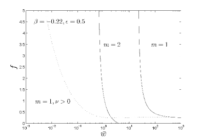
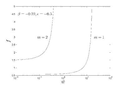
Figure 1: (a) The physically allowed combinations of $\bar{w}$ (a measure for the disc temperature and magnetic pressure together) and $f$ (a measure for the background dark matter halo potential) for global stationary MHD perturbation configurations with the scale-free index $\beta=-0.22$ and $\epsilon=0.5$ (i.e., the disc self-gravity overtakes the magnetic tension force); the two solid curves separately stand for $m=1$ and $m=2$ aligned cases, while the dotted curve stands for $m=1$ unaligned case and the curves of $m\geq 2$ unaligned cases are unphysical. Note that different points on the dotted curve have different $\nu$ values and the bifurcation point is at (461.2, 0.2764) in the ($\bar{w},f$) diagram. (b) The same as in panel (a), except for $\epsilon=-0.5$ (i.e., the magnetic tension force overtakes the disc self-gravity) and thus the requirement $f>0.5$. The unaligned logarithmic spiral cases all become unphysical.

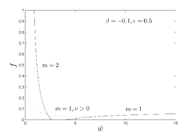
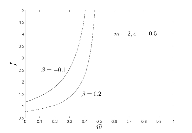
Figure 2: (a) The physically allowed combinations of $\bar{w}$ (a measure of the disc temperature and magnetic pressure together) and $f$ (a measure of the background dark matter halo potential) for global stationary MHD perturbation configurations when the scale-free index $\beta=-0.1$ and $\epsilon=0.5$ (i.e., the horizontal disc self-gravity overtakes the magnetic tension force); the two solid curves separately stand for $m=1$ and $m=2$ aligned cases, while the dotted curve stands for $m=1$ unaligned case and the curves of $m\geq 2$ unaligned cases are all unphysical. The bifurcation point for $m=1$ case from the aligned to unaligned case is at (6.383, 0.02475). (b) The same as in panel (a), except for $\beta=0.2$. For the $m=1$ case, the bifurcation point is at (0.2943, 0.03955). (c) For $\epsilon=-0.5$ (i.e., the magnetic tension force overtakes the horizontal disc self-gravity), the physically allowed combinations of $\bar{w}$ and $f$ for $m=2$ and $m=1$ stationary MHD perturbation configurations with $\beta=-0.1$ and $\beta=0.2$. The aligned and unaligned cases of $m=1$ and the unaligned case of $m=2$ are all unphysical. Two solid curves stand for $m=2$ aligned case with $\beta=-0.1$ and $\beta=0.2$, respectively.

A more straightforward relation between $f$ and $\bar{w}$ can be simply expressed as

$$f=\epsilon\left(\frac{C_{1}}{\bar{w}-C_{a}}-C_{2}\right)\ ,$$ (65)

where $C_{1}$ and $C_{2}$ are defined explicitly by

$$C_{1} \equiv \frac{[1+(1+2\beta)C_{a}]Y_{m}(\beta)}{2\beta Y_{0}(\beta)}\ ,$$ (66)

$$C_{2} \equiv 1-\frac{(1+2\beta)Y_{m}(\beta)}{2\beta Y_{0}(\beta)}\ .$$ (67)

When $\epsilon=0$ corresponding to the situation of the magnetic tension exactly cancelled by the horizontal disc self-gravity, equation (56) and background equilibrium relation (33) then give

$$\bar{w}=C_{a}\ ,\qquad\qquad f=b_{0}^{2}[1+(1+2\beta)C_{a}]\ .$$ (68)

In order to ensure $C_{a}\geq 0$, we need $m\geq 2$ or $\beta\in(-1/2,\ -0.2071)$. Thus for $\epsilon=0$, aligned MHD perturbation configurations of $m\geq 2$ can exist, while the $m=1$ mode can only exist when $\beta\in(-1/2,\ -0.2071)$. As the horizontal disc self-gravity is cancelled by the magnetic tension force, only the dark matter halo potential resists the centrifugal force, the thermal pressure force and the magnetic pressure force to maintain the disc equilibrium. Note that when $\epsilon=0$, we have a fixed $\bar{w}$ and $b_{0}^{2}$ is determined by $f$ as compared to the expression of $b_{0}^{2}$ using $w$ and $f$ in equation (33). This situation is strikingly similar to those of low-mass discs ($f\rightarrow\infty$) referred to by Syer & Tremaine (1996). Such a similarity can be easily understood because when $\epsilon=0$, the horizontal disc self-gravity is completely cancelled by the magnetic tension force and the effective $f$ (defined as the ratio of the force from the background halo to the force from the disc) apparently approaches infinity. In a certain sense, $\epsilon=0$ represents a critical point separating two qualitatively different cases. For $0<\epsilon\leq 1$, the magnetic tension force is weaker than the horizontal self-gravity force of the disc, while for $\epsilon<0$, the magnetic tension force becomes stronger than the horizontal self-gravity of the disc. One would expect systems dominated by magnetic Lorentz force or gravity to show different physical properties.

When $0<\epsilon\leq 1$, the entire analysis here parallels the corresponding part of aligned discs in Syer & Tremaine (1996), because we can simply take $f/\epsilon$ and $\Theta w$ to replace their $f$ and the $w$ variables, respectively. In other words, the two factors $1/\epsilon$ and $\Theta$ can be regarded as linear rescaling factors of $f$ and $w$ variables when the magnetic tension force is weaker than the horizontal disc self-gravity force.

When $\epsilon<0$, the magnetic tension force becomes stronger than the horizontal self-gravity of the disc. From the background rotational MHD equilibrium condition (33), the gravitational potential of a dark matter halo must exist and be strong enough in order to create an MHD disc equilibrium in the first place. As already noted earlier, physical constraints on the disc system are $\bar{w}\geq 0$ and $f\geq\max\{0,\ -\epsilon\}$. With these requirements, we can infer the physically allowed part of a hyperbolic curve of equation (65) in the ($\bar{w},\ f$) diagram and determine the relevant range of $\bar{w}$.

For the aligned cases, we reach the following conclusions drawn from the analysis detailed in Appendix A. For $m\geq 2$ MHD perturbation modes (bar-like), we have $\bar{w}\in(C_{a}\ ,\ C_{a}+C_{1}/C_{2}]$ when $0<\epsilon\leq 1$ (see Figs. 1a, 2a, 2b) and $\bar{w}\in[0\ ,\ C_{a})$ when $\epsilon<0$ (see Figs. 1b, 2c). For $m=1$ MHD perturbation modes with $0<\epsilon\leq 1$, we have $\bar{w}\in(C_{a}\ ,\ +\infty)$ when $\beta\in(-1/2\ ,\ -0.2071)$ (see Fig. 1a), $\bar{w}\in[C_{1}/C_{2}+C_{a}\ ,\ +\infty)$ when $\beta\in(-0.2071\ ,\ 0)$ (see Fig. 2a), and $\bar{w}\in[0\ ,\ C_{1}/C_{2}+C_{a}]$ when $\beta\in(0\ ,\ 1/2)$ (see Fig. 2b). For $m=1$ MHD perturbation modes with $\epsilon<0$, only when $\beta\in(-1/2\ ,\ -0.2071)$ and $\bar{w}\in[0\ ,\ C_{a})$ can global stationary MHD perturbation patterns possibly exist (see Fig. 1b).

We now discuss several special cases below.

The case of $\beta=0$ corresponds to a flat rotation curve of constant $v_{\theta 0}$ and a singular isothermal disc (SID) under scale-free conditions (Shu et al. 2000; Lou 2002; Lou & Shen 2003; Shen & Lou 2004a; Lou & Zou 2004, 2006; Lou & Wu 2005; Lou & Bai 2006). Using the asymptotic expression $\Gamma(x)\sim x^{-1}$ in the limit of $x\rightarrow 0$, we write equation (65) as

$$f=-\frac{\epsilon(m-1)(m\bar{w}-m-2)}{(m^{2}\bar{w}-m^{2}+2)}=\frac{\epsilon(m-1)}{m}\left[\frac{2(m+1)}{m^{2}\bar{w}-(m^{2}-2)}-1\right]$$ (69)

where $\beta=0$ has been set. One can readily see that $f=0$ for an arbitrary $\bar{w}$ when $m=1$ and $\beta=0$. In other words, an isopedically magnetized isolated disc with a flat rotation curve supports an $m=1$ MHD perturbation mode for an arbitrary Mach number (Syer & Tremaine 1996; Shu et al. 2000; Lou 2002; Lou & Shen 2003; Lou & Zou 2004, 2006; Lou & Wu 2005). For $m\geq 2$ MHD perturbation modes, we have $\bar{w}\in(1-2/m^{2}\ ,\ 1+2/m]$ when $0<\epsilon\leq 1$ and $\bar{w}\in[\ 0\ ,\ 1-2/m^{2})$ when $\epsilon<0$, respectively.

Another singular case appears when $\beta=(1-\sqrt{2})/2=-0.2071$ and $m=1$. According to equation (56), we have $b_{0}=0$ corresponding to a nonrotating disc. In other words, for a disc with a scale-free index $\beta=-0.2071$, it has to be nonrotational in order to support a stationary $m=1$ MHD perturbation mode.

7 Global Stationary Unaligned Logarithmic Spirals with $\nu\neq 0$

For unaligned logarithmic spiral cases, the isodensity contours of MHD perturbations entail a systematic phase shift in azimuth as $R$ increases, which gives a logarithmic spiral pattern. Unaligned stationary logarithmic spirals involve both azimuthal and radial propagations of MHD density waves. For a constant radial flux of angular momentum, we require $\beta_{1}=\Re(\beta^{\prime})=1/4$. To be general, we take $\beta_{1}$ and $\beta$ to be two different parameters.

7.1 Nonaxisymmetric Disturbances with $m\neq 0$

For $m\neq 0$, the corresponding relation (57) can be written as

$$\epsilon B=b_{0}^{2}(\bar{w}-C)\ ,$$ (70)

where

$$B\equiv\frac{Y_{m}(\beta^{\prime})}{2\beta Y_{0}(\beta)}=B(m,\ \nu,\ \beta_{1};\ \beta)\ ,\qquad\qquad C\equiv\frac{m^{2}-2(1-\beta)}{[m^{2}+2(\beta+\beta^{\prime}-2\beta^{\prime 2})]}=C(m,\ \nu,\ \beta_{1};\ \beta)\ .$$ (71)

Here, parameters $b_{0}^{2}$, $\bar{w}$ and $\epsilon$ are all real, while functions $B$ and $C$ may be complex in general. We then have

$$\epsilon\Re(B)=b_{0}^{2}[\bar{w}-\Re(C)]\ ,\qquad\qquad\epsilon\Im(B)=-b_{0}^{2}\Im(C)\ .$$ (72)

We can also write the real and imaginary parts of $C$, $\Re(C)$ and $\Im(C)$, explicitly as

$$\Re(C) = \frac{[m^{2}-2(1-\beta)](m^{2}+2\beta+2\beta_{1}-4\beta_{1}^{2}+\nu^{2})}{(m^{2}+2\beta+2\beta_{1}-4\beta_{1}^{2}+\nu^{2})^{2}+\nu^{2}(1-4\beta_{1})^{2}}\ ,$$ (73)

$$\Im(C) = \frac{\nu(1-4\beta_{1})[m^{2}-2(1-\beta)]}{(m^{2}+2\beta+2\beta_{1}-4\beta_{1}^{2}+\nu^{2})^{2}+\nu^{2}(1-4\beta_{1})^{2}}\ .$$ (74)

Based on the analysis of Appendix A and equations (73) and (74), we notice the following relations that $C(m,\ -\nu,\ \beta_{1};\ \beta)=C^{\ast}(m,\ \nu,\ \beta_{1};\ \beta)$, $B(m,\ -\nu,\ \beta_{1};\ \beta)=B^{\ast}(m,\ \nu,\ \beta_{1};\ \beta)$, $B(m,\ \nu,\ \beta_{1};\ \beta)=B(-m,\ \nu,\ \beta_{1};\ \beta)$ and $C(m,\ \nu,\ \beta_{1};\ \beta)=C(-m,\ \nu,\ \beta_{1};\ \beta)$, where the asterisk ^∗ indicates the complex conjugate operation. Therefore, equation (72) remains valid for $\pm\nu$ and $\pm m$. This conclusion can be seen as a manifestation of the anti-spiral theorem (Lynden-Bell & Ostriker 1967), which states that trailing spiral and leading spiral share the same solution forms under stationary and time-reversible conditions. Therefore, there is no loss of generality to consider $m\geq 0$ and $\nu>0$.

When $\beta\in(-1/2,\ 1/2)$ and $m\geq 1$, it is clear that $m^{2}-2(1-\beta)\neq 0$. According to equation (74), we thus have $\Im(C)=0$ only if $\nu=0$ or $\beta_{1}=1/4$. Obviously, $\nu=0$ corresponds to the aligned case as has been discussed already. The requirement $\beta_{1}=1/4$ implies a constant radial flux of angular momentum associated with logarithmic spiral MHD perturbations.

When $\epsilon=0$, we need $\beta_{1}=1/4$ and $m\geq 2$ to satisfy equation (72).

7.1.1 Discs with $\beta_{1}=1/4$

When $\beta_{1}=1/4$, equation (70) becomes real and appears as

$$\frac{\epsilon\pi}{2\beta Y_{0}(\beta)}\left|\frac{\Gamma(m/2+1/4+\mathrm{i}\nu/2)}{\Gamma(m/2+3/4+\mathrm{i}\nu/2)}\right|^{2}=\frac{(f+\epsilon)}{[1+(1+2\beta)\bar{w}]}\left[\bar{w}-\frac{m^{2}-2(1-\beta)}{(m^{2}+2\beta+1/4+\nu^{2})}\right]\ ,$$ (75)

which can be further transformed into

$$f=\epsilon\left(\frac{D_{1}}{\bar{w}-D_{0}}-D_{2}\right)\qquad\mbox{or}\qquad(f+\epsilon D_{2})(\bar{w}-D_{0})=\epsilon D_{1}\ ,$$ (76)

where the three coefficients $D_{0}$, $D_{1}$ and $D_{2}$ are explicitly defined by

$$D_{0} \equiv \frac{[m^{2}-2(1-\beta)]}{(m^{2}+2\beta+1/4+\nu^{2})}\ ,$$

$$D_{1} \equiv \frac{\pi}{2\beta Y_{0}(\beta)}\left|\frac{\Gamma(m/2+1/4+\mathrm{i}\nu/2)}{\Gamma(m/2+3/4+\mathrm{i}\nu/2)}\right|^{2}\frac{[2m^{2}(1+\beta)+4\beta^{2}-7/4+\nu^{2}]}{(m^{2}+2\beta+1/4+\nu^{2})}\ ,$$

$$D_{2} \equiv 1-\frac{\pi(1+2\beta)}{2\beta Y_{0}(\beta)}\left|\frac{\Gamma(m/2+1/4+\mathrm{i}\nu/2)}{\Gamma(m/2+3/4+\mathrm{i}\nu/2)}\right|^{2}\ .$$

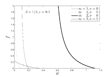
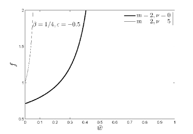
Figure 3: (a) Given the background scale-free index $\beta=1/4$ and $\epsilon=0.5$ (i.e., the horizontal disc self-gravity overtakes the magnetic tension force), the physically allowed combinations of $\bar{w}$ (a measure of the disc temperature and magnetic pressure together) and $f$ (a measure of the background dark matter halo potential) for $m=1$ and $m=2$ global stationary MHD perturbation configurations of the perturbation scale-free index $\beta_{1}=1/4$ disc with $\nu=0$ (aligned) and $\nu=5$ (unaligned), respectively. Two solid curves stand for $m=2$ MHD perturbation mode and two dotted curves stand for $m=1$ MHD perturbation mode. (b) The same as panel (a), except for $\epsilon=-0.5$ (i.e., the magnetic tension force overtakes the horizontal disc self-gravity). Note that a $m=1$ MHD perturbation mode does not exist for $\epsilon<0$.

A relationship is thus established by equation (76) between $\bar{w}$ and $f$. By specifying parameters $m$, $\nu$ and $\beta$, this relation gives rise to a hyperbolic curve in the $(\bar{w},f)$ diagram. From Appendix B, we thus draw the following conclusions. For $m\geq 2$ MHD perturbation modes, we have $\bar{w}\in(D_{0}\ ,\ D_{0}+D_{1}/D_{2}]$ when $0<\epsilon\leq 1$ (see Fig. 3a) and $\bar{w}\in[0\ ,\ D_{0})$ when $\epsilon<0$ (see Fig. 3b); for $m=1$ MHD perturbation modes, we have $\bar{w}\in[0\ ,\ D_{0}+D_{1}/D_{2}]$ when $0<\epsilon\leq 1$ (see Fig. 3a) and these modes do not exist when $\epsilon<0$.

When $\epsilon=0$, we have a fixed $\bar{w}$ as $\bar{w}=D_{0}$ and thus $m=1$ MHD perturbation mode cannot exist for a negative $D_{0}$. A relationship between $f$ and $b_{0}^{2}$ can be established in the form of

$$f=b_{0}^{2}\left[1+(1+2\beta)D_{0}\right]\ ,$$ (77)

which is similar to equation (68) for the aligned cases.

7.1.2 Stationary Logarithmic Spiral Patterns in Discs with $\beta_{1}\neq 1/4$

When $\beta_{1}\neq 1/4$, we have $\Im(C)\neq 0$. Equation (70) is then complex, giving rise to two real equations. From equation (72), we solve for $\bar{w}$ and $f$ to obtain

$$\bar{w} = \Re(C)-\frac{\Re(B)\Im(C)}{\Im(B)}\ ,$$ (78)

$$f = -\epsilon\left\{\left[1+(1+2\beta)\left(\Re(C)-\frac{\Re(B)\Im(C)}{\Im(B)}\right)\right]\frac{\Im(B)}{\Im(C)}+1\right\}\ .$$ (79)

From extensive numerical computations, we gain the following useful information. First, $\Re(B)>0$ and decreases with increasing $\nu$. Secondly, $\Im(B)>0$ for $-1/2<\beta_{1}<1/4$ and $\Im(B)<0$ for $1/4<\beta_{1}<1/2$, respectively.

We emphasize here that the $\bar{w}$ and $f$ solutions (78) and (79) give a specific point in the $(\bar{w},f)$ diagram, which differs from the aligned case with $\nu=0$ or $\beta_{1}=1/4$ discs whose real dispersion relation gives a hyperbolic curve in the $(\bar{w},f)$ diagram. Under the conditions $\nu\neq 0$ and $\beta_{1}\neq 1/4$ (non-constant radial flux of angular momentum, see Appendix G), dispersion relation (70) is generally complex, corresponding to two constraints (i.e., real and imaginary parts of equation 70) on the combination of $\bar{w}$ and $f$ and reducing a solution curve to a solution point in the $(\bar{w},f)$ diagram (see Figs. 1a, 2a, 2b).

Finally, we reach the following conclusions numerically: $\bar{w}<0$ when $m\geq 2$; for $m=1$ MHD perturbation modes, $\bar{w}$ remains always positive, while $f>0$ only for $\epsilon>0$. Therefore, global stationary spiral MHD perturbation configurations with $\beta_{1}\neq 1/4$ can only exist for $m=1$ MHD perturbation modes and when $\epsilon>0$ (see Figs. 1a, 2a, 2b).

7.1.3 Bifurcation Points from Aligned Cases

The sequence of stationary logarithmic spirals with $\nu\in(0,\ +\infty)$ bifurcates from the aligned discs with $\nu=0$ at the critical point where $\nu\rightarrow 0$. When $\nu$ becomes small, $\Im(B)$ and $\Im(C)$ may be replaced by $-\nu(\partial B/\partial\beta^{\prime})/2$ and $-\nu(\partial C/\partial\beta^{\prime})/2$ respectively, where the two first derivatives are evaluated in the limit of $\nu\rightarrow 0\ \ (\beta^{\prime}=\beta_{1})$.

Therefore at the bifurcation point (indicated by a subscript ${}_{\mbox{bif}}$ of a physical variable), equations (72) become

$$\epsilon B=b_{0}^{2}(\bar{w}-C)\ ,\qquad\qquad\epsilon\frac{\partial B}{\partial\beta^{\prime}}=-b_{0}^{2}\frac{\partial C}{\partial\beta^{\prime}}\ ,$$ (80)

where all quantities are evaluated at $\nu=0$ ($\beta^{\prime}=\beta_{1}$). Eliminating $b_{0}^{2}$ between the above two expressions, we obtain

$$\bar{w}_{\mbox{bif}}=-\left(\frac{\partial C}{\partial\beta^{\prime}}\right)\left(\frac{\partial\ln B}{\partial\beta^{\prime}}\right)^{-1}+C\ ,$$

where the derivatives are evaluated at $\nu=0$ or $\beta^{\prime}=\beta_{1}$.

We then obtain

$$\bar{w}_{\mbox{bif}}=\frac{2(1-4\beta_{1})[m^{2}+2(\beta-1)]}{[(m^{2}+2\beta+2\beta_{1}-4\beta_{1}^{2})^{2}\Psi_{m}(\beta_{1})]}+\frac{[m^{2}+2(\beta-1)]}{(m^{2}+2\beta+2\beta_{1}-4\beta_{1}^{2})}\ ,$$ (81)

where

$$\Psi_{m}(z)\equiv\psi\left(\frac{m}{2}+z\right)+\psi\left(\frac{m}{2}-z+1\right)-\psi\left(\frac{m}{2}-z+\frac{1}{2}\right)-\psi\left(\frac{m}{2}+z+\frac{1}{2}\right)\ ,$$

and $\psi(z)$ is the digamma function (e.g., Shen & Lou 2004). Once $\bar{w}$ is determined, the expression of $f$ follows from equation (65), namely

$$f_{\mbox{bif}}=\epsilon\left\{\frac{Y_{m}(\beta_{1})}{2\beta Y_{0}(\beta)}\left[(1+2\beta)+\frac{(m^{2}+2\beta+2\beta_{1}-4\beta_{1}^{2})[m^{2}(1+\beta)-(1-\beta_{1})+2(\beta^{2}-\beta_{1}^{2})]}{(1-4\beta_{1})[m^{2}+2(\beta-1)]}\Psi_{m}(\beta_{1})\right]-1\right\}\ .$$ (82)

Together, this pair of $\bar{w}_{\mbox{bif}}$ (equation 81) and $f_{\mbox{bif}}$ (equation 82) gives a specific point in the $(\bar{w},f)$ diagram which signifies the bifurcation place between the aligned and unaligned sequences (see Figs. 1a, 2a, 2b). Numerical explorations have demonstrated that when $m\geq 2$, $\bar{w}_{\mbox{bif}}<0$, while for $m=1$, both $\bar{w}_{\mbox{bif}}$ and $f_{\mbox{bif}}$ are positive. Therefore only for $m=1$ MHD perturbation modes, the bifurcation point is physically meaningful.

7.2 Marginal Instability of Axisymmetric Disturbances ($m=0$)

When $m=0$, dispersion relation (59) can be written as

$$\frac{\epsilon Y_{0}(\beta^{\prime})}{2\beta Y_{0}(\beta)}=b_{0}^{2}\left[\bar{w}-\frac{(\beta-1)}{\beta_{1}(1-2\beta_{1})+\nu^{2}/2-\mathrm{i}(1-4\beta_{1})\nu/2}\right]\ .$$ (83)

We adopt $\beta_{1}=1/4$ to make equation (83) real, namely

$$\frac{\epsilon\pi{\mathcal{N}}_{0}(\nu)}{\beta Y_{0}(\beta)}=b_{0}^{2}\left[\bar{w}+\frac{8(1-\beta)}{(1+4\nu^{2})}\right]\ ,$$ (84)

where ${\mathcal{N}}_{0}(\nu)$ is the Kalnajs function defined by equation (15). From equation (84), we then obtain $\bar{w}$ as

$$\bar{w}\equiv\frac{1}{D^{2}}=\frac{1}{(1+2\beta)}\left[\mathcal{N}_{0}(\nu)-\frac{8Y_{0}(\beta)\beta(1-\beta)(1+f/\epsilon)}{\pi(1+4\nu^{2})}\right]\bigg{/}\left[\frac{\beta Y_{0}(\beta)(1+f/\epsilon)}{\pi(1+2\beta)}-{\mathcal{N}}_{0}(\nu)\right]\ ,$$ (85)

where $D^{2}$ is defined as $1/\bar{w}=1/(\Theta w)$, which is the same as the $D^{2}$ introduced by Shu et al. (2000). When $\epsilon<0$, we require $\epsilon+f>0$ and thus $1+f/\epsilon<0$. Therefore when $\epsilon<0$ with $1+f/\epsilon<0$, $\bar{w}$ remains always negative according to equation (85). When $\epsilon=0$ in equation (84), there is no global stationary configuration, as in the situation of $\epsilon<0$.

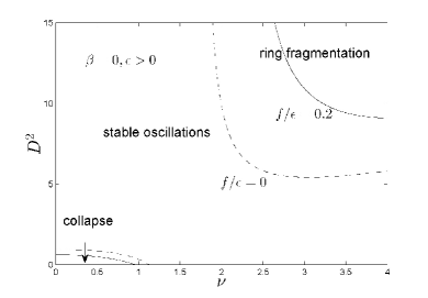
Figure 4: The axisymmetric ($m=0$) marginal instability curves of $D^{2}$ $(1/\bar{w})$ (the reciprocal of the disc temperature and magnetic pressure together) versus $\nu$ (the dimensionless radial wavenumber) with different ratio $f/\epsilon$ equal to 0 (dashed curves) and 0.2 (solid curves), respectively, for specified values of the perturbation scale-free index $\beta_{1}=1/4$ and the background scale-free index $\beta=0$. We take $\epsilon>0$ (i.e., the disc self-gravity overtakes the magnetic tension force). For $\epsilon<0$ (i.e., the magnetic tension force dominates the disc self-gravity), the instability does not exist. Note that both the Jeans collapse and ring fragmentation unstable regions shrink with increasing $f/\epsilon$.

When equation (85) is displayed in the $(\nu,\ D^{2})$ diagram, the curves correspond to the marginal instability ($\omega=0$). Here $\nu$ represents the radial wavenumber of MHD perturbations, and a smaller $\nu$ signifies a larger perturbation scale. Also, $D^{2}$ is the square of the rotational Mach number, and a larger $D^{2}$ thus signifies a faster rotation. Using equation (52), we can analyze stability properties of the $(\nu,\ D^{2})$ diagram in different parameter regimes separated by the marginal instability curves (Shu et al. 2000; Lou 2002; Lou & Shen 2003; Shen & Lou 2004b; Lou & Wu 2005; Lou & Zou 2006). Here $\omega^{2}>0$ means stability and $\omega^{2}<0$ means instability, respectively. According to equation (52), we see that when $\epsilon<0$, $\omega^{2}$ remains always positive so that the disc is completely linearly stable to axisymmetric perturbations at all wavelengths. As a consequence, the marginal stability curve in Figure 4 does not exist when $\epsilon<0$; in other words, both Jeans collapse and ring fragmentation instabilities are suppressed (i.e., lower-left curves become negative and upper-right curves move to infinity).

For $\epsilon>0$, we discuss only a special case of $\beta=0$ as an example of illustration, which corresponds to the SID case (Shu et al. 2000; Lou 2002; Lou & Shu 2003; Lou & Wu 2005). A more general treatment (Shen & Lou 2004a, b) will be given in a forthcoming paper especially aiming at the axisymmetric instability.

Knowing the asymptotic limiting expression $\beta Y_{0}(\beta)\rightarrow\pi$ as $\beta\rightarrow 0$, we obtain $1/\bar{w}$ as

$$\frac{1}{\bar{w}}\equiv D^{2}=\frac{(1+f/\epsilon)-{\mathcal{N}}_{0}(\nu)}{{\mathcal{N}}_{0}(\nu)-8(1+f/\epsilon)/(1+4\nu^{2})}\ .$$ (86)

From Appendix F, the solution curves of equation (86) separate the $(\nu,\ D^{2})$ diagram into three or two regimes. The lower-left corner and the upper-right corner are the unstable regions with $\omega^{2}<0$. The lower-left corner corresponding to MHD perturbations of large radial spatial scales represents the region of Jeans collapse instability modified by the disc rotation and the isopedic magnetic field, while the upper-right corner corresponding to perturbations of smaller radial spatial scales represents the region of the MHD ring fragmentation instability (Lou & Fan 1998a; Shu et al. 2000; Lou 2002). Sandwiched between these two unstable regimes is the stable region of $\omega^{2}>0$ (Shen & Lou 2004a; see Fig. 4 for direct visual impressions).

We can also demonstrate that as $f$ increases or $\epsilon$ decreases, both the MHD Jeans collapse and ring fragmentation instability regions tend to shrink. In other words, an enhanced background dark matter halo potential or a stronger isopedic magnetic field tend to squash instabilities both in small ( MHD ring fragmentation) and large (MHD Jeans collapse) spatial scales. In particular, when $1+f/\epsilon>{\mathcal{N}}_{0}(0)=4.337$, the MHD Jeans collapse instability region disappears. In contrast, the MHD ring fragmentation region always exists. For example, a cold disc ($\bar{w}=0$ or $D^{2}\rightarrow+\infty$) will always subject to the ring fragmentation instability. Our numerical explorations are supportive of some conclusions of numerical simulation results of Miller (1978), namely, a certain level of velocity dispersion is necessarily required for the disc stability, and furthermore, a massive dark matter halo cannot stabilize a ‘cold’ disc galaxy completely.

In short, we come to the conclusion that a massive background dark matter halo (i.e., a high $f$ ratio) and a strong isopedic magnetic field (i.e., a small $\epsilon$) tend to make the magnetized gas disc more stable against axisymmetric MHD disturbances.

8 Conclusions, Summary and Discussion

Using the standard linearization procedure for MHD perturbations in a rotating disc, we have in a more general manner constructed global stationary MHD perturbation configurations (i.e., small deviations from the axisymmetric background) for both aligned and unaligned logarithmic spiral patterns in a razor-thin scale-free disc system embedded in an axisymmetric dark matter halo potential and with an isopedic magnetic field almost vertically threaded through the gas disc plane. The stability analysis of axisymmetric MHD perturbations is performed in a disc of flat rotation curve with $\beta=0$ (i.e., SID) as an example of illustration. The most important and interesting contribution of our paper is that we integrate several essential aspects, such as isopedic magnetic field and dark matter halo, into the disc dynamics and adopt an analytic approach for the stability analysis. A generalized relationship is achieved and some interesting properties directly derived from the relationship have been revealed.

As global stationary MHD perturbation configurations may represent transitions between stabilities to instabilities and vice versa (Shu et al. 2000), we can use the obtained global MHD perturbation configurations to explore initial conditions for possible instabilities and the dynamical evolution of a razor-thin scale-free disc system. Thus, a more realistic magnetized disc system to model actual spiral galaxies may provide sensible physical information. Since the systematic galactic observations by Rubin et al. (1982) and Kent (1986, 1987, 1988), the massive dark matter halo becomes an indispensable component for models of disc galaxies, which are referred to as a partial disc system (e.g., Binney & Tremaine 1987; Syer & Tremaine 1996; Shu et al. 2000; Lou & Shen 2003; Shen & Lou 2004a; Lou & Wu 2005; Lou & Bai 2006). Meanwhile, the ubiquitous presence of galactic magnetic fields requires a serious and systematic consideration of the magnetized gas disc in a typical disc spiral galaxy in order to trace the dynamic evolution in a more realistic manner. In our idealized MHD model, the more massive dark matter halo is presumed to be axisymmetric and compatible with the scale-free conditions, while the magnetic field is taken to be of an isopedic geometry. Our MHD disc model does include several essential elements of disc galaxies and have already shown some interesting and intricate phenomena. In short, self-gravity and thermal pressure of a rotating scale-free disc, the axisymmetric gravitational potential of a dark matter halo and the isopedic magnetic field across the disc are synthesized together in our current model framework.

In the model analysis, we consider the self-gravity component in the disc without the usual WKBJ or tight-winding approximation and allow the background disc scale-free index $\beta$ and the perturbation scale-free index $\beta_{1}$ to be different in general. In other words, the long-range gravitational effect has been taken into account in full. Therefore equation (50) is fairly comprehensive and rigorous linear dispersion relationship, from which much information can be gained, such as the WKBJ relationship in Appendix B, global stationary MHD dispersion relations (56) and (58). By choosing different parameters, equation (50) is sufficiently general to include aligned ($\nu=0$) and unaligned ($\nu\neq 0$) cases, as well as axisymmetric ($m=0$) and nonaxisymmetric ($m\neq 0$) cases.

The MHD discs are specified in a range for the background scale-free index $\beta\in(-1/2,\ 1/2)$ [n.b., $\beta\in(-1/4,\ 1/2)$ for warm discs only], the inverse-square magnetosonic Mach number (disc temperature and magnetic pressure together) $\bar{w}>0$, the ratio of the gravity force of the dark matter halo to the unperturbed disc gravity force $f>0$ and the gravity dilution (due to the magnetic tension force) factor $\epsilon\leq 1$. Meanwhile, MHD perturbations are characterized by the perturbation scale-free index $\beta_{1}\in(-1/2,\ 1/2)$, azimuthal wavenumber $m$ (integer) and radial wavenumber $\nu$. With all these parameters in physical ranges, we proceed to construct global stationary MHD perturbation configurations in a specific background disc (characterized by $\beta$, $\bar{w}$, $f$ and $\epsilon$ parameters) under a specific perturbation (characterized by $\beta_{1}$, $m$ and $\nu$). In comparison with the WKBJ dispersion relation (Appendix B), the marginal instability of axisymmetric MHD disturbances is examined for discs with flat rotation curves ($\beta=0$).

Our conclusions are summarized below.

(i) Aligned Cases with $\nu=0$.

For global stationary aligned MHD perturbations, we take $\beta_{1}=\beta$, although the disc system does allow for $\beta_{1}\neq\beta$ in general. The axisymmetric ($m=0$) aligned MHD perturbation represents purely a slight rescaling of the axisymmetric background (Lou & Shen 2003; Shen & Lou 2004a; Lou & Zou 2004, 2006; Lou & Wu 2005). For both $\epsilon>0$ and $\epsilon<0$ regimes, the global $m\geq 2$ stationary MHD perturbation configurations exist when $\bar{w}$ varies within a certain limited region (see Figs. 1, 2 and C1). For neutral $m=1$ MHD perturbation modes with $\epsilon>0$, there are three types of relations between $\bar{w}$ and $f$ when $\beta$ parameter falls within the three intervals $(-1/2,\ -0.2071)$, $(-0.2071,\ 0)$ and $(0,\ 1/2)$, respectively (see Figs. 1a, 2a, 2b and Fig. C2). When $\epsilon<0$, neutral $m=1$ MHD perturbation modes can only exist for $\beta\in(-1/2,\ -0.2071)$ (see Figs. 1b and C2). Having specified values of $m$, $\beta$ and $\epsilon$ parameters, the global stationary MHD perturbation configurations can be displayed in the ($\bar{w},\ f$) diagram. One point in the ($\bar{w},\ f$) diagram then corresponds to one specific global stationary MHD perturbation configuration, and all of these points together constitute continuously a hyperbolic curve in the ($\bar{w},\ f$) diagram. A detailed description and figures can be found in Appendix C.

(ii) Unaligned Cases with $\nu\neq 0$.

To maintain a constant radial flux of angular momentum associated with MHD perturbations (e.g., Goldreich & Tremaine 1979; Shen et al. 2005), the perturbation scale-free index $\beta_{1}$ should be set to $1/4$. Furthermore, the $\beta_{1}=1/4$ stationary MHD perturbation configurations, in which the angular momentum flux is constant (see Appendix G), restrict parameter $\bar{w}$ to a certain limited region for $m\geq 1$ neutral MHD perturbations. In particular, the $m=1$ neutral MHD perturbation mode does not exist for $\epsilon<0$. For given values of $m$, $\beta$, $\nu$ and $\epsilon$ parameters, global stationary MHD perturbation configurations correspond to a hyperbolic curve shown in the ($\bar{w},\ f$) diagram (see Fig. 3); this is similar to the aligned MHD perturbation configurations. Details of analysis can be found in Appendix D. When $\beta_{1}\neq 1/4$ (i.e., non-constant radial flux of angular momentum), the dispersion relation becomes complex and its imaginary part gives an additional constraint. Thus for given values of $m$, $\beta$, $\beta_{1}$, $\nu$ and $\epsilon$ parameters, the continuous point set of global stationary MHD perturbation configurations shrink from an extended one-dimensional curve to a single point in the ($\bar{w},\ f$) diagram (see Figs. 1a, 2a, 2b). Numerical explorations show that only $m=1$ lopsided MHD perturbation modes exist.

(iii) Marginal Instabilities for Axisymmetric Disturbances with $m=0,\ \beta_{1}=1/4$ and $\nu\neq 0$.

Given a special value of $\beta=0$, we have shown that the increase of a dark matter halo mass (larger $f$ parameter) or of magnetic field flux (smaller $\epsilon>0$ parameter) can squeeze both the Jeans collapse and ring fragmentation instability regions. In the regime of $\epsilon<0$, the MHD disc becomes stable for axisymmetric MHD perturbations of all radial wavelengths, according to the WKBJ analysis.

From the model results summarized above, we can see the existence of an isopedic magnetic field can greatly influence the global stationary MHD perturbation configurations in a scale-free disc system, as well as the axisymmetric stability properties. When $0<\epsilon<1$, an isopedic magnetic field gives rise to an effective modification factor on the gravitational constant $G$, from $G$ to $\epsilon G$ (Shu et al. 2000), and an effective enhancement factor on the sound speed $v_{s}$ (thermal pressure), from $v_{s}$ to $\sqrt{\Theta}v_{s}$. In the absence of the dark matter halo, $\epsilon$ has to be positive in order to maintain a disc equilibrium. In other words, the magnetic field tension force cannot dominate the self-gravity component in the disc plane. However, a massive dark matter halo exerts an extra gravity force to hold the magnetized disc together, allowing the magnetic tension force to overtake the self-gravity component in the disc plane, corresponding to a situation of $\epsilon<0$. In the parameter regime $\epsilon<0$, we can no longer regard the isopedic magnetic field as a modification but must face an entirely new physical situation involving several interesting features in a strongly magnetized disc system. An interesting example is to derive the MHD WKBJ relation in equation (52) for the instability of axisymmetric disturbances ($m=0$). When $\epsilon<0$, we always have $\omega^{2}>0$, indicating the disc system being stable for axisymmetric MHD disturbances of all wavelengths.

Starting from the case of $\epsilon<0$, we may extend the same idea to more generalized situations. As a system has a strong magnetic field attached to plasma or gas, the magnetic field would have torn the system apart in the absence of an external massive dark matter halo potential. Two possible physical examples come into mind: the hot magnetized gas trapped in the centre of a galaxy cluster (e.g., Makino 1997; Dolag et al. 2001; Hu & Lou 2004) and the accretion disc around a SMBH (e.g., Kudoh et al. 1996; Kaburaki 2000) where strong magnetic field may exist. The former can be perceived in reference to a quasi-spherical system in which a hot gas is mainly confined by the dark matter potential and the hot gas itself is strongly magnetized. Our current model offers another possibility in that a more or less flat gas disc system in rotation can be primarily confined by a dark matter potential and the gas disc itself is isopedically magnetized with a considerable strength. By observing the existence of unusually strong magnetic field in a localized region, we may predict some ‘unseen’ dark matter components of the system. For instance, if a source region has strong cyclotron or synchrotron emissions with much reduced optical emissions, the scenario outlined above may provide a possible explanation.

Fujita & Kato (2005) proposed that Weibel instability may be responsible for generating strong magnetic fields in galaxies and clusters of galaxies at redshift as high as $z\sim 10$; in such a scenario, the magnetic field can play a crucial role in forming galaxies and galaxy clusters. Our model results, especially those for a strong magnetic field (i.e., $\epsilon<0$), offer several interesting clues for the dynamics of galaxy or galaxy cluster formation. With extensive observations for magnetic fields in clusters of galaxies (Taylor et al. 2006), a more sensible MHD model may be constructed and tested.

The final point of interest involves the radial flux of angular momentum. If the radial flux of angular momentum is constant, only the central part will collapse and the outer portion of a disc is stable. If the radial flux of angular momentum increases with increasing $R$, the disc mass at all radii will lose their angular momentum by interacting with stationary MHD density waves, and hence gradually spiral inward and drift towards the centre. In this situation, not only the central part, but also the entire disc drifts inward. For a single rotating disc embedded in an axisymmetric dark matter halo, the angular momentum of the disc system is conserved. In the presence of an external nonaxisymmetric potential, such as a companion or satellite galaxy, this conservation no longer holds. Implications of this issue will be investigated further.

Appendix A Several Properties of Function $Y_{m}(\beta^{\prime})$

The function $Y_{m}(\beta^{\prime})$ can be explicitly expressed as

$$Y_{m}(\beta^{\prime})=\frac{\pi\Gamma(z_{1})\Gamma(z_{2})}{\Gamma(z_{1}+1/2)\Gamma(z_{2}+1/2)}\$$ (87)

in terms of Gamma function $\Gamma(\cdots)$, where

$$z_{1}=m/2-\beta^{\prime}+1/2\ ,\qquad z_{2}=m/2+\beta^{\prime}\ ,\qquad\beta^{\prime}=\beta_{1}-{\mathrm{i}\nu}/{2}\ .$$ (88)

Since $\Gamma(z^{\ast})=\Gamma(z)^{\ast}$ with the asterisk $\ast$ denoting the complex conjugate operation, it then follows that

$$Y_{m}(\beta^{\prime\ast})=\frac{\pi\Gamma(z_{1}^{\ast})\Gamma(z_{2}^{\ast})}{\Gamma(z_{1}^{\ast}+1/2)\Gamma(z_{2}^{\ast}+1/2)}=\frac{\pi\Gamma(z_{1})^{\ast}\Gamma(z_{2})^{\ast}}{\Gamma(z_{1}+1/2)^{\ast}\Gamma(z_{2}+1/2)^{\ast}}=Y_{m}(\beta^{\prime})^{\ast}\ .$$ (89)

Using the recursion relation $\Gamma(z)\Gamma(1-z)=\pi/\sin(\pi z)$, we obtain

$$\begin{split}Y_{-m}(\beta^{\prime})=\frac{\pi\Gamma(1/2-z_{2})\Gamma(1/2-z_{1})}{\Gamma(1-z_{2})\Gamma(1-z_{1})}=Y_{m}(\beta^{\prime})\frac{\sin[\pi(1-z_{2})]\sin[\pi(1-z_{1})]}{\sin[\pi(1/2-z_{2})]\sin[\pi(1/2-z_{1})]}\qquad\qquad\\ \qquad\qquad=Y_{m}(\beta^{\prime})\frac{\cos[\pi(z_{1}-z_{2})]-\cos[\pi(z_{1}+z_{2})]}{\cos[\pi(z_{1}-z_{2})]+\cos[\pi(z_{1}+z_{2})]}=Y_{m}(\beta^{\prime})\ .\end{split}$$

That is, $Y_{m}(\beta^{\prime})$ function is symmetric or even with respect to the subscript $m$.

According to the Stirling formula, the asymptotic series of Gamma function $\Gamma(z)$ is given by

$$\Gamma(z)=(2\pi)^{1/2}e^{-z}z^{z-1/2}\left(1+\frac{1}{12z}+\frac{1}{288z^{2}}+\cdots\right)\ .$$ (90)

In terms of asymptotic series expansion (90), $\Gamma(z_{1})$, $\Gamma(z_{2})$, $\Gamma(z_{1}+1/2)$ and $\Gamma(z_{2}+1/2)$ are given by

$$\Gamma(z_{1}) = (2\pi)^{1/2}e^{-z_{1}}z_{1}^{z_{1}-1/2}\left[1-\frac{\mathrm{i}}{6\nu}+O(\nu^{-2})\right]\ ,$$

$$\Gamma(z_{2}) = (2\pi)^{1/2}e^{-z_{2}}z_{2}^{z_{2}-1/2}\left[1+\frac{\mathrm{i}}{6\nu}+O(\nu^{-2})\right]\ ,$$

$$\Gamma(z_{1}+1/2) = (2\pi)^{1/2}e^{-(z_{1}+1/2)}(z_{1}+1/2)^{z_{1}}\left[1-\frac{\mathrm{i}}{6\nu}+O(\nu^{-2})\right]\ ,$$

$$\Gamma(z_{2}+1/2) = (2\pi)^{1/2}e^{-(z_{2}+1/2)}(z_{2}+1/2)^{z_{2}}\left[1+\frac{\mathrm{i}}{6\nu}+O(\nu^{-2})\right]\ .$$

To the leading order, we then have $Y_{m}(\beta^{\prime})$ in the form of

$$Y_{m}(\beta^{\prime})=e\pi z_{1}^{z_{1}-1/2}z_{2}^{z_{2}-1/2}(z_{1}+1/2)^{-z_{1}}(z_{2}+1/2)^{-z_{2}}[1+O(\nu^{-2})]\ .$$ (91)

A formula frequently used in the following analysis is given below

$$z^{z^{\prime}}=\exp\left[z^{\prime}(\ln|z|+\mathrm{i}\arg z)\right]\ ,$$ (92)

where $z$ and $z^{\prime}$ are two arbitrary complex numbers and $\arg z$ is the principal value of the argument $z$.

In addition, we have

$$\ln\left|z_{i}+1/2\right| = \ln\left\{\sqrt{[\Re(z_{i}+1/2)]^{2}+[\Im(z_{i}+1/2)]^{2}}\right\}=\ln(|\nu|/2)+{2[\Re(z_{i}+1/2)]^{2}}/{\nu^{2}}+O(\nu^{-4})\ ,\quad(\hbox{for }i=1,2)$$

$$\ln\left|z_{i}\right| = \ln\left\{\sqrt{[\Re(z_{i})]^{2}+[\Im(z_{i})]^{2}}\right\}=\ln(|\nu|/2)+{2[\Re(z_{i})]^{2}}/{\nu^{2}}+O(\nu^{-4})\ ,\qquad\qquad(\hbox{for }i=1,2)$$

and

$$\arg z_{1} = \ \hbox{ }\ \mbox{sgn}(\nu)\pi/2-{2\Re(z_{1})}/{\nu}+O(\nu^{-3})\ ,$$

$$\arg z_{2} = -\mbox{sgn}(\nu)\pi/2+{2\Re(z_{2})}/{\nu}+O(\nu^{-3})\ ,$$

$$\arg\left(z_{1}+1/2\right) = \ \hbox{ }\ \mbox{sgn}(\nu)\pi/2-{2\Re(z_{1}+1/2)}/{\nu}+O(\nu^{-3})\ ,$$

$$\arg\left(z_{2}+1/2\right) = -\mbox{sgn}(\nu)\pi/2+{2\Re(z_{2}+1/2)}/{\nu}+O(\nu^{-3})\ ,$$

where sgn stands for the signum function. Hence, we arrive at the following two relations

$$L_{1}=(z_{1}-1/2)\ln|z_{1}|+(z_{2}-1/2)\ln|z_{2}|-z_{1}\arg\ln|z_{1}+1/2|-z_{2}\ln|z_{2}+1/2|=-\ln(|\nu|/2)-{\mathrm{i(1-4\beta_{1})}}/{2\nu}+O(\nu^{-2})\ ,$$

and

$$L_{2}=(z_{1}-1/2)\arg z_{1}+(z_{2}-1/2)\arg z_{2}-z_{1}\arg\left(z_{1}+1/2\right)-z_{2}\arg\left(z_{2}+1/2\right)=\mathrm{i}+{(1-4\beta_{1})}/{\nu}+O(\nu^{-2})\ .$$

From formula (92), it is easy to see

$$\exp(L_{1}+\mathrm{i}L_{2})=z_{1}^{z_{1}-1/2}z_{2}^{z_{2}-1/2}(z_{1}+1/2)^{-z_{1}}(z_{2}+1/2)^{-z_{2}}\ .$$

Finally, we derive

$$Y_{m}(\beta^{\prime})=\pi\exp\left[-\ln\frac{|\nu|}{2}+\frac{\mathrm{i(1-4\beta_{1})}}{2\nu}+O(\nu^{-2})\right][1+O(\nu^{-2})]=\frac{2\pi}{|\nu|}\left[1+\frac{\mathrm{i(1-4\beta_{1})}}{2\nu}\right]+O(\nu^{-3})\ .$$ (93)

Appendix B The WKBJ or Tight-Winding Approximation

According to equation (50), we have

$$\frac{(\hat{\omega}+mb_{0})^{2}-2(1-\beta)b_{0}^{2}}{w\Theta b_{0}^{2}-\epsilon c_{0}GY_{m}(\beta^{\prime})} = \nu^{2}+m^{2}+2\beta_{1}-4\beta_{1}^{2}+\mathrm{i}\nu\left[4\beta_{1}-1+\frac{2(1+\beta)\hat{\omega}(\hat{\omega}+mb_{0})}{(\hat{\omega}+mb_{0})^{2}-2(1-\beta)b_{0}^{2}}\right]$$

$$\qquad\qquad+\frac{2\beta mb_{0}}{\hat{\omega}+mb_{0}}+\frac{4(1+\beta)\left[mb_{0}-\beta_{1}(\hat{\omega}+mb_{0})\right]\hat{\omega}}{(\hat{\omega}+mb_{0})^{2}-2(1-\beta)b_{0}^{2}}\ ,$$

which can be further cast into the form of

$$\frac{R^{2}[(\omega+m\Omega_{0})^{2}-\kappa_{0}^{2}]}{\Theta v_{s0}^{2}-\epsilon R\Sigma_{0}GY_{m}(\beta^{\prime})} = \nu^{2}+m^{2}+2\beta_{1}-4\beta_{1}^{2}+\mathrm{i}\nu\left[4\beta_{1}-1+\frac{2(1+\beta)\omega(\omega+m\Omega_{0})}{(\omega+m\Omega_{0})^{2}-\kappa_{0}^{2}}\right]$$ (94)

$$\qquad\qquad+\frac{2\beta m\Omega_{0}}{\omega+m\Omega_{0}}+\frac{4(1+\beta)\left[m\Omega_{0}-\beta_{1}(\omega+m\Omega_{0})\right]\omega}{(\omega+m\Omega_{0})^{2}-\kappa_{0}^{2}}\ .$$

First, it is clear that equation (94) is singular when $\omega+m\Omega=0$ and $(\omega+m\Omega_{0})^{2}-\kappa_{0}^{2}=0$. These correspond to the corotation resonance and the inner and outer Lindblad resonances (Goldreich & Tremaine 1979). In our analysis, such singular points do not appear due to the stationary condition $\omega=0$.

In the regime of $\nu\gg\mbox{max}(m,\ \omega,\ 1)$, equation (94) can be significantly simplified to

$$\frac{(\omega+m\Omega_{0})^{2}-\kappa_{0}^{2}}{\Theta v_{s0}^{2}-\epsilon R\Sigma_{0}GY_{m}(\beta^{\prime})}=\left(\frac{\nu}{R}\right)^{2}[1+O(\nu^{-1})]\ .$$ (95)

From Appendix A, we know $Y_{m}(\beta^{\prime})\approx 2\pi/|\nu|$ in the limit of $\nu\gg\mbox{max}(m,\ 1)$. By defining the radial wavenumber $k$ as $\nu/R$, we can rearrange equation (95) into the following form

$$(\omega+m\Omega_{0})^{2}=\kappa_{0}^{2}+k^{2}\Theta v_{s0}^{2}-2\pi\epsilon G|k|\Sigma_{0}\ ,$$ (96)

which shares the classic WKBJ form (Lou & Fan 1998a). According to equation (95), dispersion relation (96) has an error of the order of $O(\nu^{-1})$. From equation (94), we note that errors can be reduced to $O(\nu^{-2})$ when $\beta_{1}=1/4$ and $\omega\rightarrow 0$; for these special cases, a more accurate dispersion relation can be obtained (Shu et al. 2000).

Appendix C Aligned Cases

For aligned cases, we begin with the expression

$$f=\epsilon\left(\frac{C_{1}}{\bar{w}-C_{a}}-C_{2}\right)\ ,$$ (97)

where the three coefficients $C_{a}$, $C_{1}$, and $C_{2}$ are explicitly defined by

$$C_{a} \equiv \frac{m^{2}-2(1-\beta)}{m^{2}+4\beta(1-\beta)}\ ,$$ (98)

$$C_{1} \equiv \frac{[1+(1+2\beta)C_{a}]Y_{m}(\beta)}{2\beta Y_{0}(\beta)}\ ,$$ (99)

$$C_{2} \equiv 1-\frac{(1+2\beta)Y_{m}(\beta)}{2\beta Y_{0}(\beta)}\ .$$ (100)

Clearly, we can write equation (97) in the form of $(f+\epsilon C_{2})(\bar{w}-C_{a})=\epsilon C_{1}$. When plotted on a two-dimensional diagram of $(\bar{w},f)$, this relation takes a hyperbolic shape.

The three constraints $\bar{w}\geq 0$, $f\geq 0$ and $f+\epsilon\geq 0$ can also be effectively written as $\bar{w}\geq 0$ and $f\geq\max\{0,-\epsilon\}$.

In short, equation (97) depicts a hyperbolic curve in the $(\bar{w},\ f)$ diagram for specified $m$, $\beta$ and $\epsilon$ parameters. The two constraints $\bar{w}\geq 0$ and $f\geq\max\{0,-\epsilon\}$ enclose a region of physical interest. In other words, only the enclosed parts of the hyperbolic curve are physically meaningful.

For different combinations of $m$, $\beta$ and $\epsilon$, we will discuss whether the physically meaningful solutions of the hyperbolic curves exist and the possible ranges of the curves, which are expressed as ranges of $\bar{w}$. From the hyperbolic curves, the ranges of $f$ can be readily calculated for the given ranges of $\bar{w}$. Note that $m$ is a positive integer, $\beta\in(-1/2,\ 1/2)$ and $\epsilon\leq 1$. The special case of $\epsilon=0$ is investigated in the main text.

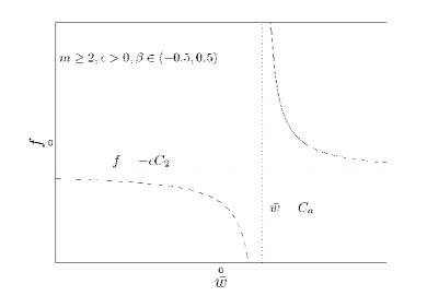
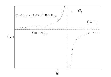
Figure 5: Combinations of $\bar{w}$ (a measure for the disc temperature and magnetic pressure together) and $f$ (a measure for the background dark matter halo potential strength) for $m\geq 2$ global stationary MHD perturbation configurations when $\beta\in(-1/2,\ 1/2)$. Panel (a) shows the case of $\epsilon>0$ (i.e., the disc self-gravity overtakes the magnetic tension force) and panel (b) is the case of $\epsilon<0$ (i.e., the magnetic tension force overtakes the disc self-gravity). The physically meaningful parts are plotted in solid curve and the unphysical parts are plotted in dashed lines. In panel (b), the dash-dotted line indicates the constraint on $f$ when $\epsilon<0$, due to $f+\epsilon\geq 0$. Several asymptotes are given in dotted lines, $f=-\epsilon C_{2}$ and $\bar{w}=C_{a}$.

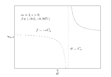
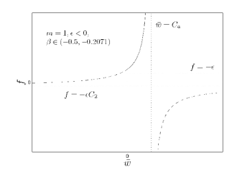
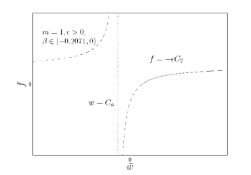
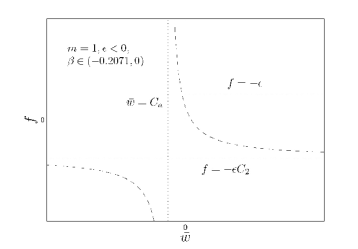
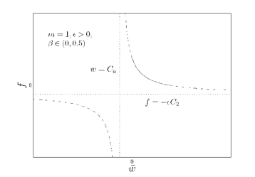
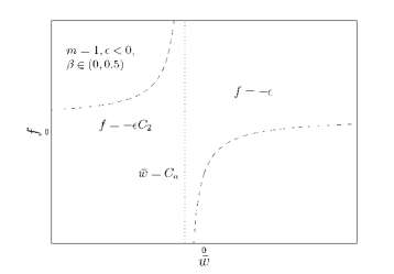
Figure 6: Combinations of $\bar{w}$ (a measure for the disc temperature and magnetic pressure together) and $f$ (a measure for the background dark matter halo potential strength) for $m=2$ global stationary MHD perturbation configurations with $\beta\in(-1/2,\ 1/2)$. Panels (a), (c), (e) are the cases of $\epsilon>0$ (the disc self-gravity overtakes the magnetic tension force), and panels (b), (d), (f) are the cases of $\epsilon<0$ (the magnetic tension force overtakes the disc self-gravity). The range of $\beta$ is separated into three different segments: panels (a) and (b) are for $\beta\in(-1/2,\ -0.2071)$; panels (c) and (d) are for $\beta\in(-0.2071,\ 0)$; panels (e) and (f) are for $\beta\in(0,\ 1/2)$. The physically meaningful parts are plotted in solid curves and the unphysical parts are shown in dashed lines. The dash-dotted lines indicate the constraint on $f$ with $\epsilon<0$, due to $f+\epsilon\geq 0$. Several asymptotes are shown in dotted lines, $f=-\epsilon C_{2}$ and $\bar{w}=C_{a}$.

C.1 Cases of $m\geq 2$

For cases of $m\geq 2$, our numerical calculations show that $1/2\leq C_{a}<1$, $C_{1}>0$ and $1/3<C_{2}<1$. The case $C_{a}=1/2$ is achieved for $m=2$ and $\beta=0$.

When $0<\epsilon\leq 1$, the constraints are $f\geq 0$ and $\bar{w}\geq 0$ [see panel (a) of Fig. C1]. We can further infer

$$f\geq 0\ ,\qquad\bar{w}\geq 0\qquad\Rightarrow\quad\frac{C_{1}}{(\bar{w}-C_{a})}\geq C_{2}\quad\Rightarrow\qquad\bar{w}\in\left(C_{a}\ ,\ C_{a}+\frac{C_{1}}{C_{2}}\right]\ .$$ (101)

When $\epsilon<0$, the constraints are $f+\epsilon\geq 0$ and $\bar{w}\geq 0$ [see panel (b) of Fig. C1]. We can further infer

$$f+\epsilon\geq 0\ ,\qquad\bar{w}\geq 0\qquad\Rightarrow\qquad\mbox{max}\left\{C_{a}+\frac{C_{1}}{(C_{2}-1)}\ ,\ 0\right\}\leq\bar{w}<C_{a}\qquad\Rightarrow\qquad\bar{w}\in[0,\ C_{a})\ .$$ (102)

C.2 Cases of $m=1$

When $m=1$, both coefficients $C_{a}$ and $C_{1}$ may become singular at $\beta=(1-\sqrt{2})/2=-0.2071$. It follows that $C_{a}>0$ for $\beta\in(-1/2,\ -0.2071)$ and $C_{a}<0$ for $\beta\in(-0.2071,\ 1/2)$, respectively. We also have $C_{1}>0$ for $\beta\in(-1/2,\ -0.2071)\cup(0,\ -1/2)$ and $C_{1}<0$ for $\beta\in(-0.2071,\ 0)$, respectively. Finally, $C_{2}<0$ for $\beta\in(-1/2,\ 0)$ and $C_{2}>0$ for $\beta\in(0,\ 1/2)$, respectively. We now consider several subcases separately.

C.2.1 The subcase of $\beta\in(-1/2,\ -0.2071)$ with $C_{a}>0\ ,\ C_{1}>0\ ,\ C_{2}<0$ .

When $0<\epsilon\leq 1$,

$$f\geq 0\ ,\qquad\bar{w}\geq 0\qquad\Rightarrow\qquad\bar{w}\in(C_{a},\ +\infty)\ ,$$ (103)

and the range of $\bar{w}$ can be identified in panel (a) of Fig. C2.

When $\epsilon<0$,

$$f+\epsilon\geq 0\ ,\qquad\bar{w}\geq 0\qquad\Rightarrow\quad\mbox{max}\left\{C_{a}+\frac{C_{1}}{C_{2}-1}\ ,\ 0\right\}\leq\bar{w}\leq C_{a}\qquad\Rightarrow\qquad\bar{w}\in[\ 0,\ C_{a}\ )\ ,$$ (104)

and the range of $\bar{w}$ can be identified in panel (b) of Fig. C2.

C.2.2 The subcase of $\beta\in(-0.2071,\ 0)$ with $C_{a}<0\ ,\ C_{1}<0\ ,\ C_{2}<0$ .

When $0<\epsilon\leq 1$, we infer

$$f\geq 0\ ,\quad\bar{w}\geq 0\quad\Rightarrow\quad\bar{w}\geq\mbox{max}\left\{C_{a}+\frac{C_{1}}{C_{2}}\ ,\ 0\right\}\quad\Rightarrow\quad w\in\left[C_{a}+\frac{C_{1}}{C_{2}}\ ,\ +\infty\right)\ ,$$ (105)

and the range of $\bar{w}$ can be identified from panel (c) of Fig. C2.

When $\epsilon<0$, we infer

$$f+\epsilon\geq 0\ ,\quad\bar{w}\geq 0\quad\Rightarrow\quad C_{a}\leq\bar{w}\leq C_{a}+\frac{C_{1}}{C_{2}-1}=\frac{-1}{1+2\beta}\ ,\quad\bar{w}\geq 0\quad\Rightarrow\quad\mbox{Such a }\bar{w}\mbox{ cannot exist}\ ,$$ (106)

and no curve is within the physically allowed region in panel (d) of Fig. C2.

C.2.3 The subcase of $\beta\in(0,\ 1/2)$ with $C_{a}<0\ ,\ C_{1}>0\ ,\ C_{2}>0$ .

When $0<\epsilon\leq 1$, we infer

$$f\geq 0\ ,\quad\bar{w}\geq 0\quad\Rightarrow\quad\max\{C_{a}\ ,\ 0\}\leq\bar{w}\leq C_{a}+\frac{C_{1}}{C_{2}}\quad\Rightarrow\quad\bar{w}\in\left[0,\ C_{a}+\frac{C_{1}}{C_{2}}\right]\ ,$$ (107)

and the range of $\bar{w}$ can be seen from panel (e) of Figure C2.

When $\epsilon<0$, we infer

$$f+\epsilon\geq 0\ ,\quad\bar{w}\geq 0\quad\Rightarrow\quad\bar{w}<C_{a}\ ,\quad\bar{w}\geq 0\quad\Rightarrow\quad\mbox{Such a }\bar{w}\mbox{ cannot exist}\ ,$$ (108)

and no curve is within the physically permitted region in panel (f) of Figure C2.

Appendix D Several Properties of $\beta_{1}=1/4$ Discs

For a disc system with $\beta_{1}=1/4$, the global stationary dispersion relationship for MHD perturbations can be transformed into

$$f=\epsilon\left(\frac{D_{1}}{\bar{w}-D_{0}}-D_{2}\right)\qquad\qquad\mbox{or}\qquad\qquad(f+\epsilon D_{2})(\bar{w}-D_{0})=\epsilon D_{1}\ ,$$ (109)

where

$$D_{0} \equiv \frac{[m^{2}-2(1-\beta)]}{(m^{2}+2\beta+1/4+\nu^{2})}\ ,$$ (110)

$$D_{1} \equiv \frac{\pi}{2\beta Y_{0}(\beta)}\left|\frac{\Gamma(m/2+1/4+\mathrm{i}\nu/2)}{\Gamma(m/2+3/4+\mathrm{i}\nu/2)}\right|^{2}\frac{[2m^{2}(1+\beta)+4\beta^{2}-7/4+\nu^{2}]}{(m^{2}+2\beta+1/4+\nu^{2})}\ ,$$ (111)

$$D_{2} \equiv 1-\frac{\pi(1+2\beta)}{2\beta Y_{0}(\beta)}\left|\frac{\Gamma(m/2+1/4+\mathrm{i}\nu/2)}{\Gamma(m/2+3/4+\mathrm{i}\nu/2)}\right|^{2}\ .$$ (112)

Numerical computations show the following results: $-8<D_{0}<0$ for $m=1$ and $0<D_{0}<1$ for $m\geq 2$, respectively; in all circumstances, $D_{1}\geq 0$ and $D_{1}=0$ occurs when $m=1$, $\beta=-1/4$ and $\nu=0$; in all circumstances, $0\leq D_{2}<1$ and $D_{2}=0$ occurs when $m=1$, $\beta=-1/4$ and $\nu=0$. Note that $\beta\in(-1/2,\ 1/2)$.

Given $m$, $\nu$, $\beta$ and $\epsilon$ parameters, equation (109) represents a hyperbolic curve in the $(\bar{w},\ f)$ diagram. Two physical constraints are $\bar{w}\geq 0$ and $f\geq\max\{0,-\epsilon\}$, enclosing the physically meaningful parts of the hyperbolic curve expressed as an area of $\bar{w}$.

The case of $\epsilon=0$ is special, in which $f$ becomes arbitrary and $\bar{w}=D_{0}$. As constrained by $\bar{w}\geq 0$, neutral $m=1$ MHD perturbation mode cannot exist in $\epsilon=0$ discs.

D.1 Cases with $m\geq 2$

In these cases, we have $0<D_{0}<1$, $D_{1}>0$ and $0<D_{2}<1$ for $m\geq 2$. When $0<\epsilon\leq 1$, the two physical constraints are $f\geq 0$ and $\bar{w}\geq 0$. We therefore infer

$$f\geq 0\ ,\qquad\bar{w}\geq 0\qquad\Rightarrow\qquad\frac{D_{1}}{\bar{w}-D_{0}}\geq D_{2}\qquad\Rightarrow\qquad\bar{w}\in\left(D_{0}\ ,\ D_{0}+\frac{D_{1}}{D_{2}}\right]\ .$$ (113)

When $\epsilon<0$, the two physical constraints are $f+\epsilon\geq 0$ and $\bar{w}\geq 0$. We then infer

$$f+\epsilon\geq 0\ ,\quad\bar{w}\geq 0\quad\Rightarrow\quad\mbox{max}\left\{D_{0}+\frac{D_{1}}{D_{2}-1}\ ,\ 0\right\}\leq\bar{w}<D_{0}\quad\Rightarrow\quad\bar{w}\in[\ 0,\ D_{0})\ .$$ (114)

The schemata of the above two cases ($\epsilon>0$ and $\epsilon<0$) are the same as panels (a) and (b) of Fig. C1, respectively.

D.2 Cases with $m=1$

In these cases, we have $D_{0}<0$, $D_{1}>0$ and $0<D_{2}<1$ for $m=1$; the $D_{1}=0$ and $D_{2}=0$ cases will be discussed separately below. When $0<\epsilon\leq 1$, we infer

$$f\geq 0\ ,\quad\bar{w}\geq 0\quad\Rightarrow\quad\frac{D_{1}}{\bar{w}-D_{0}}\geq D_{2}\quad\Rightarrow\quad\bar{w}\in\left[0\ ,\ D_{0}+\frac{D_{1}}{D_{2}}\right]\ .$$ (115)

When $\epsilon<0$, we infer

$$f+\epsilon\geq 0\ ,\quad\bar{w}\geq 0\quad\Rightarrow\quad\bar{w}<D_{0}\ ,\quad\bar{w}\geq 0\quad\Rightarrow\quad\mbox{Such a }\bar{w}\mbox{ cannot exist}\ .$$ (116)

The schemata of the above two cases ($\epsilon>0$ and $\epsilon<0$) are the same as in panels (e) and (f) of Fig. C2, respectively.

Appendix E Logarithmic Spiral Discs with $\nu\neq 0\$ and $\beta_{1}\neq 1/4$

When $\nu\neq 0$ and $\beta_{1}\neq 1/4$, a point in the ($\bar{w},\ f$) diagram is given by the two values $\bar{w}$ and $f$ explicitly expressed as

$$\bar{w} = \Re(C)-\frac{\Re(B)\Im(C)}{\Im(B)}\ ,$$ (117)

$$f = -\epsilon\left\{\left[1+(1+2\beta)\left(\Re(C)-\frac{\Re(B)\Im(C)}{\Im(B)}\right)\right]\frac{\Im(B)}{\Im(C)}+1\right\}\ ,$$ (118)

where $\Re(\cdots)$ and $\Im(\cdots)$ represent the real and imaginary parts of the argument, respectively,

$$\Re(B) \equiv \frac{\Re[Y_{m}(\beta^{\prime})]}{2\beta Y_{0}(\beta)}\ ,\qquad\qquad\Im(B)\equiv\frac{\Im[Y_{m}(\beta^{\prime})]}{2\beta Y_{0}(\beta)}\ ,$$ (119)

$$\Re(C) \equiv \frac{[m^{2}-2(1-\beta)](m^{2}+2\beta+2\beta_{1}-4\beta_{1}^{2}+\nu^{2})}{(m^{2}+2\beta+2\beta_{1}-4\beta_{1}^{2}+\nu^{2})^{2}+\nu^{2}(1-4\beta_{1})^{2}}\ ,$$ (120)

$$\Im(C) \equiv \frac{\nu(1-4\beta_{1})[m^{2}-2(1-\beta)]}{(m^{2}+2\beta+2\beta_{1}-4\beta_{1}^{2}+\nu^{2})^{2}+\nu^{2}(1-4\beta_{1})^{2}}\ .$$ (121)

In the limit of $\nu\rightarrow+\infty$, we have the following asymptotic expressions to the leading orders according to equations (93), (120) and (121), namely

$$\Re[Y_{m}(\beta^{\prime})] = \frac{2\pi}{|\nu|}[1+O(\nu^{-2})]\ ,$$ (122)

$$\Im[Y_{m}(\beta^{\prime})] = \frac{\pi(1-4\beta_{1})|\nu|}{\nu^{3}}[1+O(\nu^{-1})]\ ,$$ (123)

$$\Re(C) = \frac{m^{2}-2(1-\beta)}{\nu^{2}}[1+O(\nu^{-2})]\ ,$$ (124)

$$\Im(C) = \frac{(1-4\beta_{1})[m^{2}-2(1-\beta)]}{\nu^{3}}[1+O(\nu^{-2})]\ .$$ (125)

To the leading order of large $\nu$, we then have $\bar{w}$ and $f$ expressed as

$$\bar{w} = -\frac{m^{2}-2(1-\beta)}{\nu^{2}}[1+O(\nu^{-1})]\ ,$$ (126)

$$f = -\frac{\epsilon\pi|\nu|}{2\beta Y_{0}(\beta)[m^{2}-2(1-\beta)]}[1+O(\nu^{-1})]\ .$$ (127)

According to equations (126) and (127) with $\nu\rightarrow+\infty$, $\bar{w}<0$ when $m\geq 2$ and $\bar{w}>0$ when $m=1$, respectively. For $m=1$, $f>0$ when $\epsilon>0$ and $f<0$ when $\epsilon<0$, respectively.

The above analytical analysis based on the $\nu\rightarrow+\infty$ approximation gives the variation trends of $\bar{w}$ and $f$. But, this approximation becomes invalid when $\nu\approx 1$ or smaller. We resort to numerical experiments to probe solution properties. According to extensive numerical tests, we find that $\Re[Y_{m}(\beta^{\prime})]>0$ and $\nu(1-4\beta_{1})\Im[Y_{m}(\beta^{\prime})]>0$ when $m\geq 1$.

E.1 Cases with $m\geq 2$

When $m\geq 2\ ,$ we have $\Re(C)>0\ .$ Meanwhile, $\bar{w}$ can be written as

$$\bar{w}=\Re(C)\left\{1-\frac{\nu(1-4\beta_{1})}{(m^{2}+2\beta+2\beta_{1}-4\beta_{1}^{2}+\nu^{2})}\frac{\Re[Y_{m}(\beta^{\prime})]}{\Im[Y_{m}(\beta^{\prime})]}\right\}\ .$$ (128)

Extensive numerical results show that

$$\frac{\nu(1-4\beta_{1})}{(m^{2}+2\beta+2\beta_{1}-4\beta_{1}^{2}+\nu^{2})}\frac{\Re[Y_{m}(\beta^{\prime})]}{\Im[Y_{m}(\beta^{\prime})]}>\frac{\nu(1-4\beta_{1})}{(m^{2}+1+2\beta_{1}-4\beta_{1}^{2}+\nu^{2})}\frac{\Re[Y_{m}(\beta^{\prime})]}{\Im[Y_{m}(\beta^{\prime})]}>1\ .$$

Therefore when $m\geq 2$, we have $\bar{w}<0$ by extensive numerical explorations.

E.2 Cases with $m=1$

In these cases, we have

$$\bar{w}=\frac{-(1-2\beta)}{[(1+2\beta+2\beta_{1}-4\beta_{1}^{2}+\nu^{2})^{2}+\nu^{2}(1-4\beta_{1})^{2}]}\left\{1+2\beta+2\beta_{1}-4\beta_{1}^{2}+\nu^{2}-\nu(1-4\beta_{1})\frac{\Re[Y_{1}(\beta^{\prime})]}{\Im[Y_{1}(\beta^{\prime})]}\right\}\ .$$

Extensive numerical explorations show the following inequalities

$$1+2\beta+2\beta_{1}-4\beta_{1}^{2}+\nu^{2}-\nu(1-4\beta_{1})\frac{\Re[Y_{1}(\beta^{\prime})]}{\Im[Y_{1}(\beta^{\prime})]}<2+2\beta_{1}-4\beta_{1}^{2}+\nu^{2}-\nu(1-4\beta_{1})\frac{\Re[Y_{m}(\beta^{\prime})]}{\Im[Y_{m}(\beta^{\prime})]}<0\ ,$$

and therefore we have $\bar{w}>0\ .$

The $f$ parameter can be written as

$$f=\epsilon\left\{\frac{[1+(1+2\beta)\bar{w}]\Re(B)}{[\bar{w}-\Re(C)]}-1\right\}\ .$$ (129)

We can also derive the following relationship

$$\bar{w}-\Re(C)=-\frac{\Re(B)\Im(C)}{\Im(B)}=\frac{\nu(1-4\beta_{1})(1-2\beta)}{(1+2\beta+2\beta_{1}-4\beta_{1}^{2}+\nu^{2})^{2}+\nu^{2}(1-4\beta_{1})^{2}}\frac{\Re[Y_{1}(\beta^{\prime})]}{\Im[Y_{1}(\beta^{\prime})]}>0\ .$$

For $\epsilon<0$, we require $f+\epsilon\geq 0$ on the ground of physics. However,

$$f+\epsilon=\epsilon\left\{\frac{[1+(1+2\beta)\bar{w}]\Re(B)}{[\bar{w}-\Re(C)]}\right\}<0\ ,$$

leading to an obvious contradiction. Therefore for $\epsilon<0$, stationary $m=1$ MHD perturbation modes do not exist.

When $\epsilon>0$, the physical constraint becomes $f\geq 0$, giving the following inequalities

$$\qquad\frac{[1+(1+2\beta)\bar{w}]\Re(B)}{[\bar{w}-\Re(C)]}\geq 1\quad\Rightarrow\quad(1+2\beta)\Re(C)+1-\frac{\Im(C)}{\Im(B)}[(1+2\beta)\Re(B)-1]\geq 0\ .$$

Extensive numerical examples show that the above inequalities always hold true. We therefore infer numerically that when $\epsilon>0$ and $f>0$, stationary $m=1$ MHD perturbation neutral modes do exist.

Appendix F Axisymmetric cases

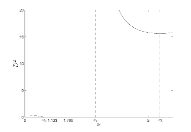
Figure 7: The axisymmetric ($m=0$) marginal instability curves (upper-right and lower-left solid curves) of $D^{2}\$ ($1/\bar{w}$) (the reciprocal of the disc temperature and magnetic pressure together) versus $\nu$ (dimensionless radial wavenumber for perturbations) for specified values of $f/\epsilon=0.5$, the scale-free index $\beta_{1}=1/4$ for perturbations and the background scale-free index $\beta=0$. Here, $\epsilon$ is taken to be positive. Five specific points, $\nu_{0}$, $1.123$, $1.760$, $\nu_{s}$ and $\nu_{b}$, can be found along the $\nu$-axis. The dashed line of $\nu_{s}$ gives the asymptote and the dash-dotted line marks the inflection point $\nu_{b}$.

When $m=0$, $\beta_{1}=1/4$ and $\beta=0$, we have

$$\frac{1}{\bar{w}}\equiv D^{2}=\frac{\mathcal{E}-{\mathcal{N}}_{0}(\nu)}{{\mathcal{N}}_{0}(\nu)-8\mathcal{E}/(1+4\nu^{2})}\ ,$$ (130)

where the Kalnajs function ${\mathcal{N}}_{0}(\nu)$ is given by definition (15) and $\mathcal{E}$ is defined as

$$\mathcal{E}=1+{f}/{\epsilon}\ .$$ (131)

Since we require inequality $f+\epsilon>0$ to hold, it follows that $\mathcal{E}=1+f/\epsilon<0$ if $\epsilon<0$. When $\mathcal{E}<0$, $\bar{w}$ remains always negative and thus unphysical. For this reason, we only focus on the situation of $\epsilon>0$ and thus $\mathcal{E}\geq 1$.

When $\mathcal{E}-{\mathcal{N}}_{0}(\nu)=0$, one has $D^{2}=0$ by equation (130). Numerical explorations show that ${\mathcal{N}}_{0}(\nu)$ decreases with increasing $\nu$. When $\mathcal{E}>{\mathcal{N}}_{0}(0)=4.377$, a positive $\mathcal{E}-{\mathcal{N}}_{0}(\nu)$ can be always guaranteed. We adopt the notation $\nu_{0}$ for the specific $\nu$ making $\mathcal{E}-{\mathcal{N}}_{0}(\nu_{0})=0$. Hence ${\mathcal{N}}_{0}(\nu_{0})=\mathcal{E}\geq 1$ corresponds to $\nu_{0}\leq 1.123$ because ${\mathcal{N}}_{0}(1.123)=1$. When $\mathcal{E}>4.377$, there is no such $\nu_{0}$ root.

The singular point $\nu_{s}$ is to make ${\mathcal{N}}_{0}(\nu_{s})-8\mathcal{E}/(1+4\nu_{s}^{2})=0$ in equation (130). Extensive numerical explorations show that $(1+4\nu^{2}){\mathcal{N}}_{0}(\nu)$ increases with increasing $\nu$. Therefore, the singular point $\nu_{s}$ should be larger than 1.760 which is the root of equation ${\mathcal{N}}_{0}(\nu)-8/(1+4\nu^{2})=0$.

From equation (130), we readily obtain

$$\frac{\partial D^{2}}{\partial\mathcal{E}}=\frac{(1+4\nu^{2}){\mathcal{N}}_{0}(\nu)(4\nu^{2}-7)}{[(1+4\nu^{2}){\mathcal{N}}_{0}(\nu)-8\mathcal{E}]^{2}}\ .$$

Thus as $\mathcal{E}=1+f/\epsilon$ increases, $D^{2}$ grows for $\nu>\sqrt{7}/2=1.323$ and decreases for $0<\nu<\sqrt{7}/2=1.323$, respectively.

Meanwhile, we can also readily derive

$$\frac{\partial D^{2}}{\partial\nu}=\frac{64\nu\mathcal{E}}{[(1+4\nu^{2}){\mathcal{N}}_{0}(\nu)-8\mathcal{E}]^{2}}\left[{\mathcal{N}}_{0}(\nu)-\frac{{\mathcal{N}}^{\prime}_{0}(\nu)(1+4\nu^{2})(4\nu^{2}-7)}{64\nu}-\mathcal{E}\right]\ .$$

We define a special value $\nu_{b}$ which is the solution $\nu$ of the following equation

$${\mathcal{N}}_{0}(\nu)-\frac{{\mathcal{N}}^{\prime}_{0}(\nu)(1+4\nu^{2})(4\nu^{2}-7)}{64\nu}-\mathcal{E}=0\ .$$ (132)

Numerical explorations clearly indicate that $\nu_{b}\geq 3.058$ which is the root of equation (132) with $\mathcal{E}=1$. With the increase of $\nu$, $D^{2}$ decreases when $\nu<\nu_{b}$ and grows when $\nu>\nu_{b}$, respectively. Moreover, numerical results show $\nu_{b}>\nu_{s}$.

Finally, we have an order of inequalities $\nu_{0}\leq 1.123<1.323<1.760\leq\nu_{s}<\nu_{b}$ (see Fig. F1). When $\nu\in[0,\ \nu_{0}]\bigcup(\nu_{s},\ +\infty)$, we have $D^{2}\geq 0$. More specifically, $D^{2}$ is a decreasing function of $\nu$ when $\nu\in[0,\nu_{0}]\bigcup(\nu_{s},\ \nu_{b})$ and an increasing function of $\nu$ when $\nu\in(\nu_{b},+\infty)$. In addition, $D^{2}$ is a decreasing function of $\mathcal{E}$ when $\nu\in[0,\ \nu_{0}]$ and an increasing function of $\mathcal{E}$ when $\nu\in(\nu_{s},\ +\infty)$. When ${\mathcal{E}}>4.377$, both $\nu_{0}$ and the range $[0,\ \nu_{0}]$ disappear. Since ${\mathcal{E}}=1+f/\epsilon$, the variation trend of $D^{2}$ as $f$ and/or $\epsilon$ change can be readily determined.

Appendix G Angular Momentum Flux Transport

In this appendix, we provide several proofs and discussions for the angular momentum flux transport associated with global coplanar MHD perturbations in a scale-free disc system with an isopedic magnetic field geometry. In general, such angular momentum flux transport contains three separate contributions (Lynden-Bell & Kalnajs 1972; Fan & Lou 1999; Shen, Liu & Lou 2005), namely, the flow advection transport $\Lambda^{\mathrm{A}}$ defined by

$$\Lambda^{\mathrm{A}}\equiv R^{2}\Sigma_{0}\int_{0}^{2\pi}\mathrm{d}\theta\Re(v_{R1})\Re(v_{\theta 1})\ ,$$ (133)

the gravity torque flux transport $\Lambda^{\mathrm{G}}$ defined by

$$\Lambda^{\mathrm{G}}\equiv\frac{1}{4\pi G}\int_{0}^{2\pi}\mathrm{d}\theta\int^{\infty}_{-\infty}\mathrm{d}zR\left[\frac{\partial\Re(\phi_{1})}{\partial\theta}\right]\left[\frac{\partial\Re(\phi_{1})}{\partial R}\right]\ ,$$ (134)

and the magnetic torque flux transport $\Lambda^{\mathrm{B}}$ defined by

$$\Lambda^{\mathrm{B}}\equiv-\frac{R^{2}}{4\pi}\int_{0}^{2\pi}\mathrm{d}\theta\int^{\infty}_{-\infty}\mathrm{d}z\Re(b_{R})\Re(b_{\theta})\ .$$ (135)

The three-dimensional gravitational potential perturbation $\phi_{1}(R,\theta,z)$ is associated with a Fourier harmonic component of a coplanar logarithmic spiral perturbation in the surface mass density $\Sigma_{1}=c_{1}R^{-2\beta^{\prime}-1}\exp(\mathrm{i}m\theta)=c_{1}R^{-2\beta-1+\mathrm{i}\nu}\exp(\mathrm{i}m\theta)=c_{1}R^{-2\beta-1}\exp[\mathrm{i}(m\theta+\nu\ln R)]$ where $c_{1}$ is a small constant amplitude coefficient. By the convention of our notations, $\phi_{1}(R,\theta,0)\equiv\Phi_{1}$ with $\Phi_{1}$ being introduced in equation (41). Here, $b_{R}$ and $b_{\theta}$ represent the two components of the magnetic field perturbation in the isopedic magnetic field. From equation (2.14) of Shu & Li (1997), we have

$$b_{R}=\frac{1}{2\pi G\Lambda}\frac{\partial\phi_{1}}{\partial R}\ ,\qquad\qquad b_{\theta}=\frac{1}{2\pi G\Lambda R}\frac{\partial\phi_{1}}{\partial\theta}\ .$$ (136)

By definition $2\pi G\Lambda\equiv\lambda{G}^{1/2}$ and $1/\lambda^{2}=1-\epsilon$, we then have

$$\Lambda^{\mathrm{B}}=-\frac{R^{2}}{4\pi}\int_{0}^{2\pi}\mathrm{d}\theta\int^{\infty}_{-\infty}\mathrm{d}z\Re(b_{R})\Re(b_{\theta})=-\frac{1}{4\pi G\lambda^{2}}\int_{0}^{2\pi}\mathrm{d}\theta\int^{\infty}_{-\infty}\mathrm{d}zR\left[\frac{\partial\Re(\phi_{1})}{\partial\theta}\right]\left[\frac{\partial\Re(\phi_{1})}{\partial R}\right]=(\epsilon-1)\Lambda^{\mathrm{G}}\ .$$ (137)

Corresponding to $\Sigma_{1}=c_{1}R^{-2\beta-1}\exp[\mathrm{i}(m\theta+\nu\ln R)]$, the gravitational potential perturbation $\phi_{1}$ can be written as (e.g., Binney & Tremaine 1987)

$$\phi_{1}(R,\theta,z)=-2\pi Gc_{1}\exp(\mathrm{i}m\theta)\int_{0}^{\infty}\mathrm{d}k\exp(-k|z|)J_{m}(kR)\int_{0}^{\infty}\mathrm{d}R^{\prime}R^{\prime-2\beta_{1}+\mathrm{i}\nu}J_{m}(kR^{\prime})\ ,$$ (138)

where $J_{m}(x)$ is the cylindrical Bessel function of order $m$ with an argument $x$. We then have

$$\Re(\phi_{1})=-2\pi Gc_{1}\int_{0}^{\infty}\mathrm{d}k\exp(-k|z|)J_{m}(kR)\int_{0}^{\infty}\mathrm{d}R^{\prime}R^{\prime-2\beta_{1}}\cos(m\theta+\nu\ln R^{\prime})J_{m}(kR^{\prime})\ .$$ (139)

where $c_{1}$ is taken to be real.

It follows immediately that

$$\frac{\partial\Re(\Phi_{1})}{\partial\theta}=2\pi Gmc_{1}\int_{0}^{\infty}\mathrm{d}k_{a}\exp(-k_{a}|z|)J_{m}(k_{a}R)\int_{0}^{\infty}\mathrm{d}R_{a}R_{a}^{-2\beta_{1}}\sin(m\theta+\nu\ln R_{a})J_{m}(k_{a}R_{a})\ ,$$ (140)

and

$$\frac{\partial\Re(\Phi_{1})}{\partial R}=-2\pi Gc_{1}\int_{0}^{\infty}\mathrm{d}k_{b}\exp(-k_{b}|z|)\left[-k_{b}J_{m+1}(k_{b}R)+\frac{m}{R}J_{m}(k_{b}R)\right]\int_{0}^{\infty}\mathrm{d}R_{b}R_{b}^{-2\beta_{1}}\cos(m\theta+\nu\ln R_{b})J_{m}(k_{b}R_{b})\ .$$ (141)

Using the following relations

$$\int^{\infty}_{-\infty}\mathrm{d}z\exp[-(k_{a}+k_{b})|z|]=2\int^{\infty}_{0}\mathrm{d}z\exp[-(k_{a}+k_{b})z]=\frac{2}{(k_{a}+k_{b})}$$ (142)

and

$$\begin{split}&\int_{0}^{2\pi}\mathrm{d}\theta\cos(m\theta+\nu\ln R_{b})\sin(m\theta+\nu\ln R_{a})\\ \qquad\qquad&\qquad=\frac{1}{2}\int_{0}^{2\pi}\mathrm{d}\theta\{\sin[\nu\ln(R_{a}/R_{b})]+\sin[2m\theta+\nu\ln(R_{a}R_{b})]\}=\pi\sin\left[\nu\ln\left(\frac{R_{a}}{R_{b}}\right)\right]\ ,\end{split}$$ (143)

we obtain the gravity torque flux transport

$$\begin{split}\Lambda^{\mathrm{G}}=-2m\pi^{2}Gc_{1}^{2}R\int^{\infty}_{0}\mathrm{d}k_{a}\mathrm{d}k_{b}\mathrm{d}R_{a}\mathrm{d}R_{b}R_{a}^{-2\beta_{1}}R_{b}^{-2\beta_{1}}J_{m}(k_{a}R_{a})J_{m}(k_{b}R_{b})\\ \times\sin\left[\nu\ln\left(\frac{R_{a}}{R_{b}}\right)\right]\frac{J_{m}(k_{a}R)}{(k_{a}+k_{b})}\left[\frac{m}{R}J_{m}(k_{b}R)-k_{b}J_{m+1}(k_{b}R)\right]\ .\end{split}$$ (144)

By taking the following integral transformations

$$x_{a}=k_{a}R\ ,\quad x_{b}=k_{b}R\ ,\quad y_{a}=\frac{R_{a}}{R}\ ,\quad y_{b}=\frac{R_{b}}{R}\quad\Rightarrow\quad k_{a}=\frac{x_{a}}{R}\ ,\quad k_{b}=\frac{x_{b}}{R}\ ,\quad R_{a}=y_{a}R\ ,\quad R_{b}=y_{b}R\ ,$$ (145)

we arrive at

$$\Lambda^{\mathrm{G}}=-2m\pi^{2}Gc_{1}^{2}R^{1-4\beta_{1}}\mathcal{M}(\beta_{1},m,\nu)\ ,$$ (146)

where the function $\mathcal{M}(\beta_{1},m,\nu)$ is defined by

$$\mathcal{M}(\beta_{1},m,\nu)\equiv\int^{\infty}_{0}\mathrm{d}x_{a}\mathrm{d}x_{b}\mathrm{d}y_{a}\mathrm{d}y_{b}(y_{a}y_{b})^{-2\beta_{1}}J_{m}(x_{a}y_{a})J_{m}(x_{b}y_{b})\sin\left[\nu\ln\left(\frac{y_{a}}{y_{b}}\right)\right]\frac{J_{m}(x_{a})}{x_{a}+x_{b}}\left[mJ_{m}(x_{b})-x_{b}J_{m+1}(x_{b})\right]\ .$$ (147)

We correct here a few errors in Appendix C of Shen et al. (2005): $J_{m}(k^{\prime}r)$ is redundant in their equations (C1), (C2) and (C4); $J_{m}(x^{\prime})$ is redundant in equation (C6) and in the expression of $\Xi^{\mathrm{G}}$ below equation (C8), and the heavy solid curve of $\Xi^{\mathrm{G}}$ in their Figure C1 is thus invalid; an extra numerical factor 2 should be multiplied in their equations (C4), (C6) and (C8), respectively.

According to equations (60) and (61), we have

$$v_{R1}=2mc_{1}R^{-2\beta_{1}+\beta}\mathcal{K}_{R}\mathrm{i}\exp[{\mathrm{i}(m\theta+\nu\ln R)}]\ ,\qquad v_{\theta 1}=-c_{1}R^{-2\beta_{1}+\beta}\mathcal{K}_{\theta}\exp[{\mathrm{i}(m\theta+\nu\ln R)}]\ ,$$ (148)

where

$$\quad\mathcal{K}_{R}\equiv\frac{\left[w\Theta b_{0}^{2}-\epsilon c_{0}GY_{m}(\beta^{\prime})\right](1-\beta^{\prime})}{c_{0}b_{0}\left[m^{2}-2(1-\beta)\right]}\ ,\qquad\qquad\mathcal{K}_{\theta}\equiv\frac{\left[w\Theta b_{0}^{2}-\epsilon c_{0}GY_{m}(\beta^{\prime})\right]\left[m^{2}-2\beta^{\prime}(1-\beta)\right]}{c_{0}b_{0}\left[m^{2}-2(1-\beta)\right]}\ .$$

We therefore come to

$$\Re(v_{R1})=-2mc_{1}R^{-2\beta_{1}+\beta}\left[\Re(\mathcal{K}_{R})\sin(m\theta+\nu\ln R)+\Im(\mathcal{K}_{R})\cos(m\theta+\nu\ln R)\right]\ ,$$ (149)

and

$$\Re(v_{\theta 1})=-c_{1}R^{-2\beta_{1}+\beta}\left[\Re(\mathcal{K}_{\theta})\cos(m\theta+\nu\ln R)-\Im(\mathcal{K}_{\theta})\sin(m\theta+\nu\ln R)\right]\ .$$ (150)

Since

$$\int^{2\pi}_{0}\mathrm{d}\theta\left[\Re(\mathcal{K}_{R})\sin(m\theta+\nu\ln R)+\Im(\mathcal{K}_{R})\cos(m\theta+\nu\ln R)\right]\left[\Re(\mathcal{K}_{\theta})\cos(m\theta+\nu\ln R)-\Im(\mathcal{K}_{\theta})\sin(m\theta+\nu\ln R)\right]$$

$$=\frac{1}{2}\int^{2\pi}_{0}\mathrm{d}\theta\left\{-\Re(\mathcal{K}_{R})\Im(\mathcal{K}_{\theta})\left[1-\cos(2m\theta+2\nu\ln R)\right]+\Re(\mathcal{K}_{\theta})\Im(\mathcal{K}_{R})\left[1+\cos(2m\theta+2\nu\ln R)\right]\right\}$$

$$=\pi\left[\Re(\mathcal{K}_{\theta})\Im(\mathcal{K}_{R})-\Re(\mathcal{K}_{R})\Im(\mathcal{K}_{\theta})\right]\ ,$$

we derive in a straightforward manner that

$$\Lambda^{\mathrm{A}}=R^{2}\Sigma_{0}\int_{0}^{2\pi}\mathrm{d}\theta\Re(v_{R1})\Re(v_{\theta 1})=2m\pi c_{1}^{2}c_{0}R^{1-4\beta_{1}}\left[\Re(\mathcal{K}_{\theta})\Im(\mathcal{K}_{R})-\Re(\mathcal{K}_{R})\Im(\mathcal{K}_{\theta})\right]\ .$$ (151)

Finally, we write the total angular momentum flux $\Lambda_{\mathrm{total}}$ as

$$\Lambda_{\mathrm{total}}=\Lambda^{\mathrm{A}}+\Lambda^{\mathrm{G}}+\Lambda^{\mathrm{B}}=\Lambda^{\mathrm{A}}+\epsilon\Lambda^{\mathrm{G}}=2mR^{1-4\beta_{1}}c_{1}^{2}\bigg{\{}\pi c_{0}\left[\Re(\mathcal{K}_{\theta})\Im(\mathcal{K}_{R})-\Re(\mathcal{K}_{R})\Im(\mathcal{K}_{\theta})\right]-\epsilon\pi^{2}G\mathcal{M}(\beta_{1},\ m,\ \nu)\bigg{\}}\ .$$ (152)

As expected when $m=0$, we have $\Lambda_{\mathrm{total}}=0$. When $\beta_{1}=1/4$, $\Lambda_{\mathrm{total}}$ is independent of $R$. We note that all these foregoing analyses are performed under the stationary assumption of $\omega=0$.

References

- (1) Balbus S. A., 2003, ARA&A, 41, 555
- (2) Balbus S. A., Hawley J. F., 1998, Rev. Mod. Phys., 70, 1
- (3) Basu S., Mouschovias T. C., 1994, ApJ, 432, 720
- (4) Beck R., Brandenburg A., Moss D., Shukurov A., Sokoloff D., 1996, ARA&A, 34, 155
- (5) Bertin G., Lin C. C., 1996, Spiral Structure in Galaxies. MIT Press, Cambridge
- (6) Binney J., Tremaine S., 1987, Galactic Dynamics. Princeton University Press, Princeton
- (7) Dolag K., Schindler S., Govoni F., Feretti, L. 2001, A&A, 378, 777
- (8) Evans N. W., Read J. C. A., 1998a, MNRAS, 300, 83
- (9) Evans N. W., Read J. C. A., 1998b, MNRAS, 300, 106
- (10) Fan Z. H., Lou Y.-Q., 1996, Nat., 383, 800
- (11) Fan Z. H., Lou Y.-Q., 1997, MNRAS, 291, 91
- (12) Fan Z. H., Lou Y.-Q., 1999, MNRAS, 307, 645
- (13) Fujita Y., Kato T. N., 2005, MNRAS, 364, 247
- (14) Goldreich P., Tremaine S., 1979, ApJ, 233, 857
- (15) Goodman J., Evans N. W., 1999, MNRAS, 309, 599
- (16) Hohl F., 1971, ApJ, 168, 343
- (17) Hu J., Lou Y.-Q., 2004, ApJ, 606, L1
- (18) Hungerford T. W., 1997, Algebra, 8th ed. Springer-Verlag, New York
- (19) Kaburaki O., 2000, ApJ, 531, 210
- (20) Kaburaki O., 2001, ApJ, 563, 505
- (21) Kalnajs A. J., 1971, ApJ, 166, 275
- (22) Kent S. M., 1986, AJ, 91, 130
- (23) Kent S. M., 1987, AJ, 93, 816
- (24) Kent S. M., 1988, AJ, 96, 514
- (25) Kudoh T., Kaburaki O., 1996, ApJ, 460, 199
- (26) Lemos J. P. S., Kalnajs A. J., Lynden-Bell D., 1991, ApJ, 375, 484
- (27) Lin C. C., Shu F. H., 1964, ApJ, 140, 646
- (28) Lin C. C., Shu F. H., 1966, Proc. Nat. Acad. Sci., 55, 229
- (29) Lin C. C., 1987, Selected Papers of C. C. Lin. World Scientific, Singapore
- (30) Lizano S., Shu F. H., 1989, ApJ, 342, 834
- (31) Lou Y.-Q., 2002, MNRAS, 337, 225
- (32) Lou Y.-Q., Fan Z. H., 2002, MNRAS, 329, L62
- (33) Lou Y.-Q., Shen Y., 2003, MNRAS, 343, 750 (astro-ph/0304270)
- (34) Lou Y.-Q., Wu Y., 2005, MNRAS, 364, 475 (astro-ph/0508601)
- (35) Lou Y.-Q., Zou Y., 2004, MNRAS, 350, 1220 (astro-ph/0312082)
- (36) Lou Y.-Q., Zou Y., 2006, MNRAS, 366, 1037 (astro-ph/0511348)
- (37) Lou Y.-Q., Bai X. N., 2006, MNRAS, in press
- (38) Lynden-Bell D., Kalnajs A. J., 1972, MNRAS, 157, 1
- (39) Lynden-Bell D., Lemos J. P. S., 1999 (astro-ph/9907093)
- (40) Lynden-Bell D., Ostriker J. P., 1967, MNRAS, 136, 293
- (41) Makino N., 1997, ApJ, 490, 642
- (42) Mestel L., 1963, MNRAS, 157, 1
- (43) Miller R. H., Prendergast K. H., Quirk W. J., 1970, ApJ, 161, 903
- (44) Miller R. H., 1978, ApJ, 224, 32
- (45) Moffatt K., 2000, Dynamo Theory, Encyclopedia of Astronomy and Astrophysics, ed. Paul Murdin (Bristol: Institute of Physics Publishing 2001)
- (46) Nakano T., 1979, PASJ, 31, 697
- (47) Ostriker J. P., Peebles P. J. E., 1973, ApJ, 186, 467
- (48) Qian E., 1992, MNRAS, 257, 581
- (49) Rubin V. C., Thonnard N. T., Ford W. K. Jr., 1982, AJ, 87, 477
- (50) Shen Y., Liu X., Lou Y.-Q., 2005, MNRAS, 356, 1333
- (51) Shen Y., Lou Y.-Q., 2003, MNRAS, 345, 1340 (astro-ph/0308063)
- (52) Shen Y., Lou Y.-Q., 2004a, MNRAS, 353, 249 (astro-ph/0405444)
- (53) Shen Y., Lou Y.-Q., 2004b, ChJAA, 4, 541 (astro-ph/0404190)
- (54) Shu F. H., Li Z.-Y., 1997, ApJ, 475, 251
- (55) Shu F. H., Laughlin G., Lizano S., Galli D., 2000, ApJ, 535, 190
- (56) Shu F. H., Tremaine S., Adams F. C., Ruden S. P., 1990, ApJ, 358, 495
- (57) Sofue Y., Fujimoto M., Wielebinski R., 1986, ARA&A, 24, 459
- (58) Syer D., Tremaine S., 1996, MNRAS, 281, 925
- (59) Taylor G. B., Gugliucci N. E., Fabian A. C., Sanders J. S., Gentile G., Allen S. W., 2006, MNRAS, 368, 1500
- (60) Toomre A., 1977, ARA&A, 15, 437
- (61) Vallée J. P., 2004, New Astronomy Reviews, 48, 763
- (62) Zang T. A., 1976, PhD thesis, MIT, Cambridge MA