Luminosity and redshift dependent quasar clustering

Abstract

We present detailed clustering measurements for a flux limited sample of $\sim 14,000$ quasars extracted from the 2dF QSO Redshift Survey (2QZ) in the redshift range $0.8<z<2.1$. After splitting the sample into three redshift bins and each of them into six luminosity intervals, we estimate the quasar projected auto and cross-correlation functions at a given redshift for separations $3\mathrel{\hbox to0.0pt{\lower 3.0pt\hbox{$\sim$}\hss}\raise 2.0pt\hbox{$<$}}r/{h^{-1}{\rm Mpc}}\mathrel{\hbox to0.0pt{\lower 3.0pt\hbox{$\sim$}\hss}\raise 2.0pt\hbox{$<$}}20$. Fitting the data with a biased CDM model and using a frequentist analysis (the $F$-test), we find that models with luminosity dependent clustering are statistically favoured at the 95 per cent confidence level for $z>1.3$. On the other hand, a number of tests based on information theory and Bayesian statistics show only marginal evidence for luminosity dependent clustering. Anyway, the quality of the data is not good enough to accurately quantify how quasar biasing depends on luminosity. We critically discuss the limitations of our dataset and show that a much larger sample is needed to rule out current models for luminosity segregation. Studying the evolution of the clustering amplitude with redshift, we detect an increase of the quasar correlation length with lookback time at the 99.3 per cent confidence level. Adopting the concordance cosmological model, we discuss the evolution of quasar biasing with cosmic epoch and show that quasars are typically hosted by dark matter haloes with mass $\sim 10^{13}M_{\odot}$.

1 Introduction

It is widely believed that quasars are powered by accretion onto supermassive black holes. However, a detailed understanding of the physical processes leading to quasar activity (and their connection with galaxy formation) is still lacking.

Simple semi-analytic models associate quasars with galaxy major mergers and assume a tight relation between their instantaneous luminosity and the mass of the central black-hole, $M_{\rm bh}$ (Kauffmann & Haehnelt 2000; Wyithe & Loeb 2003; Volonteri et al. 2003). The fraction of gas accreted onto the black hole during each merger is chosen to match the observed relation between the velocity dispersion of the bulge and $M_{\rm bh}$ (Ferrarese & Merritt 2000). This ends up producing a correlation between the quasar luminosity and the mass of the host dark-matter halo. Since the clustering properties of dark-matter halos strongly depend on their mass, the quasar clustering amplitude is thus expected to sensibly depend on luminosity.

Recent numerical simulations of galaxy mergers including black-hole accretion and feedback have cast some doubts on this picture (Springel et al. 2005). These numerical experiments suggest that a given black-hole produces quasar activity with a wide range of luminosities (Hopkins et al. 2005). During its active phase, the black-hole is most likely observed as a relatively low-luminosity quasar with a small Eddington ratio. For a short period of time, however, its emission reaches its peak value (close to the Eddington luminosity) which is indeed proportional to the mass of the powering black-hole. Based on these models, Lidz et al. (2006) conclude that quasar clustering should depend only weakly on luminosity.

From the observational point of view, only recently quasar samples have grown big enough (in terms of number of objects) to attempt the study of the clustering amplitude as a function of luminosity. By analyzing the galaxy-quasar cross-correlation at $1.8\mathrel{\hbox to0.0pt{\lower 3.0pt\hbox{$\sim$}\hss}\raise 2.0pt\hbox{$<$}}z\mathrel{\hbox to0.0pt{\lower 3.0pt\hbox{$\sim$}\hss}\raise 2.0pt\hbox{$<$}}3.5$ Adelberger & Steidel (2005) found no evidence for luminosity-dependent clustering. They used 79 quasars spanning 4.4 orders of magnitude in absolute luminosity which have been divided into 2 luminosity bins. Larger samples are obviously required to confirm this result.

Croom et al. (2002, 2005) studied the redshift-space clustering amplitude of 2dF quasars as a function of their apparent magnitude. Even though these authors initially found weak evidence for brighter QSOs being more strongly clustered, their most recent analysis shows no indication of luminosity-dependent clustering. These two studies, however, do not address the issue of luminosity dependent clustering. In fact, they consider magnitude-limited samples within a broad redshift range ($0.3<z<2.9$ corresponding to $\sim 8$ Gyr in the currently favoured cosmological model) and totally ignore any changes in the clustering signal as a function of cosmic epoch. Moreover, their redshift-space analysis complicates the interpretation of the clustering amplitudes, as the effect of non-linear peculiar velocities could also depend on luminosity and redshift. For these reasons, their null result does not necessarily imply that quasar clustering is independent of luminosity.

In this paper, which is a follow up analysis of Porciani, Magliocchetti & Norberg (2004, PMN04 hereafter), we study the clustering properties of $\sim 14,000$ quasars extracted from the complete 2dF QSO Redshift Survey (Croom et al. 2004). Our goal is to accurately measure the real-space clustering amplitude of 2dF quasars as a function of redshift and absolute luminosity. To do this, we first split our quasar sample into three redshift bins and each subsample into six luminosity intervals. We then compute, in each redshift range, the associated projected auto- and cross-correlation functions, which, by construction, are not affected by redshift space distortions.

Using the largest quasar sample presently available, our results reveal a statistically significant evolution of the clustering length with redshift (as found already in PMN04) but only weak evidence for luminosity dependent quasar clustering.

The layout of the paper is as follows. In Section 2 we describe our quasar sample and how we split it both in redshift and in luminosity. In Section 3, we measure the projected auto- and cross-correlation functions of the different subsamples. The issue of luminosity dependent clustering is addressed in Section 4. Using a Monte Carlo Markov Chain, we estimate the quasar clustering amplitude as a function of redshift and luminosity. A number of robust tests are then used to evaluate the statistical significance of the measured luminosity dependence in a given redshift range. A critical discussion of the limitations of our data and of possible future strategies is also presented here. In Section 5, we focus on the pure redshift dependence of the quasar clustering amplitude and we provide fitting functions for the evolution of the quasar correlation length and bias with cosmic epoch. All our results are summarized in Section 6.

Throughout this paper we assume a “concordance” cosmological model with mass density parameter $\Omega_{0}=0.3$ (with a baryonic contribution $\Omega_{b}=0.049$), vacuum energy density parameter $\Omega_{\Lambda}=0.7$ and present-day value of the Hubble constant $H_{0}=100\,h\,{\rm km}\,{\rm s}^{-1}\,{\rm Mpc}$ with $h=0.7$. We also adopt a cold dark matter (CDM) power spectrum with primordial spectral index $n=1$ and with normalization fixed by $\sigma_{8}$, the rms linear density fluctuation within a sphere with radius of $8$ $\,h^{-1}\,{\rm Mpc}$.

2 Quasar sample definition

The 2dF QSO Redshift Survey (2QZ) includes 23,338 quasars which span a wide redshift range ($0.3\mathrel{\hbox to0.0pt{\lower 3.0pt\hbox{$\sim$}\hss}\raise 2.0pt\hbox{$<$}}z\mathrel{\hbox to0.0pt{\lower 3.0pt\hbox{$\sim$}\hss}\raise 2.0pt\hbox{$<$}}2.9$) and are spread over 721.6 deg² on the sky (see Croom et al. 2004). In order to minimise systematic effects, we restrict our analysis to regions with spectroscopic (photometric) completeness larger than 70 (90) per cent, which limits the redshift range to $0.5<z<2.1$. Only quasars brighter than M${}_{b_{\rm J}}-5\log_{10}h=-21.7$ are considered, which ensures the exclusion of quasars for which the contribution from the host galaxy may have led to a mis-identification of the source.

In order to make a physically motivated analysis and isolate evolutionary effects, we subdivide our sample into three redshift bins. As in PMN04, we require a similar number of quasars to lie in each redshift bin and that each sub-sample covers a not too different interval of cosmic time. To better satisfy these criteria (see PMN04 fur further details), we impose an additional redshift cut so as to keep only quasars within $0.8<z<2.1$. With this selection, we end up with nearly 14,000 2QZ quasars that we split into the redshift intervals: $0.8<z<1.3$, $1.3<z<1.7$ and $1.7<z<2.1$ (containing each between $\sim~{}4300$ and $\sim~{}4900$ quasars).

To study the dependence of the quasar clustering amplitude on luminosity, we further divide each sub-sample into six complementary sets based on quasar absolute luminosity: (F25, B75), (F50, B50) and (F75, B25), where F$x$ and B$y$ correspond to the $x$ per cent faintest quasars and the $y$ per cent brightest quasars (in terms of their absolute magnitude). Table 1 lists the main properties of each sample, including the number of quasars (col. 4), the median redshift (col. 5), the absolute magnitude range (cols. 6 & 8) and the sample median absolute magnitude (col. 7).

Table 1: Main properties of our data sets. The subscripts min, max and med respectively denote the minimum, maximum and median value of a variable.

$z_{\rm min}\!\!\!\!$	$z_{\rm max}\!\!\!\!$	Data	NQSO	$z_{\rm med}\!\!\!\!$	$M_{\rm max}\!\!\!\!$	$M_{\rm med}\!\!\!\!$	$M_{\rm min}\!\!\!\!$
					$M_{b_{\rm J}}-5\log_{10}h$
0.8	1.3	F25	1232	0.93	-21.7	-22.4	-22.7
0.8	1.3	F50	2464	0.99	-21.7	-22.7	-23.2
0.8	1.3	F75	3696	1.04	-21.7	-22.9	-23.7
0.8	1.3	B75	3698	1.12	-22.7	-23.4	-25.3
0.8	1.3	B50	2466	1.14	-23.1	-23.6	-25.3
0.8	1.3	B25	1234	1.15	-23.6	-24.0	-25.3
1.3	1.7	F25	1285	1.44	-22.8	-23.3	-23.5
1.3	1.7	F50	2571	1.48	-22.8	-23.5	-23.9
1.3	1.7	F75	3857	1.49	-22.8	-23.6	-24.3
1.3	1.7	B75	3858	1.53	-23.4	-24.0	-26.0
1.3	1.7	B50	2572	1.53	-23.8	-24.3	-26.0
1.3	1.7	B25	1286	1.55	-24.3	-24.7	-26.0
1.7	2.1	F25	1081	1.83	-23.4	-23.8	-24.0
1.7	2.1	F50	2163	1.86	-23.4	-24.0	-24.3
1.7	2.1	F75	3244	1.87	-23.4	-24.1	-24.9
1.7	2.1	B75	3245	1.91	-23.9	-24.5	-26.4
1.7	2.1	B50	2163	1.91	-24.3	-24.8	-26.4
1.7	2.1	B25	1082	1.92	-24.8	-25.2	-26.4

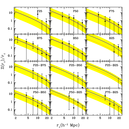
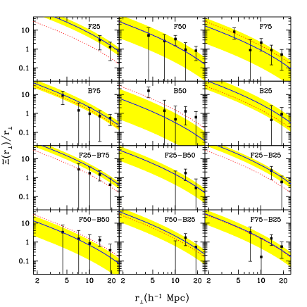
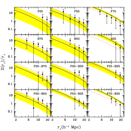
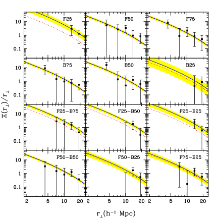
Figure 1: Top-left panel: The projected auto-correlation function (top two rows) and cross-correlation function (bottom two rows) for the low-redshift quasar samples ($0.8<z<1.3$). Only measurements obtained with more than 40 quasar pairs are plotted (filled squares with errorbars). Bins with less pairs are omitted and not considered for model fitting. For each luminosity sub-sample, the shaded band show the central 68 per cent range of best-fitting correlation functions (assuming that each luminosity interval is associated with a different bias parameter). The mean value of the marginalized bias distribution is represented with a solid line. For reference, we also plot the best-fitting correlation function for the entire low-redshift sample derived in PNM04 (dotted line). Top-right and bottom-left panels: Same as the top-left panel, but for the medium- ($1.3<z<1.7$) and high- ($1.7<z<2.1$) redshift quasar samples respectively. Bottom-right panel: As in the top-right panel but using a three-parameter model where only the B25 and F25 sub-samples have different bias parameters from all the others.

3 Quasars Clustering Analysis

3.1 Estimating the correlation functions

The simplest statistic which can be used to quantify clustering in the observed quasar distribution is the 2-point correlation function in redshift space, $\xi^{\rm q}(r_{\perp},\pi)$. To measure this quantity we first build a catalogue of unclustered points which has the same angular and radial selection function as the data. The radial selection function is obtained by heavily smoothing the observed quasar comoving distance distribution, ${\cal N}(r)$. The quasar auto-correlation function is then estimated by comparing the probability distribution of quasar and random pairs on a two-dimensional grid of separations $(r_{\perp},\pi)$. We use both the Landy-Szalay estimator (Landy & Szalay 1993) and the Hamilton estimator (Hamilton 1993):

$$\xi_{\rm{LS}}^{\rm q}=\frac{DD-2DR+RR}{RR}\;,\ \ \ \xi_{\rm{H}}^{\rm q}=\frac{DD\cdot RR}{(DR)^{2}}\,-\,1$$ (1)

where $DD$, $DR$ and $RR$ are the suitably normalised numbers of weighted data-data, data-random and random-random pairs in each bin. As expected, the two estimators give comparable answers within the errors. In what follows we only present results obtained with the Landy-Szalay estimator. Similarly, we use the appropriately symmetrized Landy-Szalay estimator to compute the quasar cross-correlation function:

$$\xi_{\rm{LS}}^{\rm q}=\frac{D_{i}D_{j}-(D_{i}R_{j}+D_{j}R_{i})+R_{i}R_{j}}{R_{i}R_{j}}\;,\ \ \$$ (2)

where $D_{i}D_{j}$, $D_{i}R_{j}$, $D_{j}R_{i}$ and $R_{i}R_{j}$ are the suitably normalised numbers of weighted data and random pairs from samples $i$ and $j$.

To avoid redshift space distortions, and determine the quasar clustering amplitude in real space, one can then use the ‘projected correlation function’ which is obtained by integrating $\xi^{\rm q}(r_{\perp},\pi)$ in the $\pi$ direction:

$$\frac{\Xi^{\rm q}(r_{\perp})}{r_{\perp}}=\frac{2}{r_{\perp}}\int_{0}^{\infty}\xi^{\rm q}(r_{\perp},\pi)\,{\rm d}\pi.$$ (3)

With the current quasar sample, we find that a reliable measure of $\xi^{\rm q}(r_{\perp},\pi)$ is only achievable on scales $\pi\mathrel{\hbox to0.0pt{\lower 3.0pt\hbox{$\sim$}\hss}\raise 2.0pt\hbox{$<$}}50$ $\,h^{-1}\,{\rm Mpc}$. In order to avoid the measured signal to be dominated by noise, we limit the integration to an upper limit, $\pi_{\rm max}$. As explained in PMN04, $\pi_{\rm max}=45$ $\,h^{-1}\,{\rm Mpc}$ is an adequate choice, and we have checked that our results are not sensitive to the precise value adopted.

As in PMN04, we use a blockwise bootstrap resampling technique to estimate the uncertainties of our clustering measurements. For each redshift interval, we divide each of the two 2QZ areas into 28 equal-volume regions, containing, within a factor of two, the same number of quasars (the minimum size of a subvolume is nearly $180h^{-1}$ Mpc for the low-redshift sample, $250h^{-1}$ Mpc for the medium-redshift sample and $220h^{-1}$ Mpc for the high-redshift; since we measure correlations on scales smaller than $20h^{-1}$ Mpc our error estimates should hardly be affected by edge-effects and/or missing large-scale structure). We build hundreds of bootstrap-samples (see §3.3), each of them composed by 56 sub-samples (28 for each 2QZ region) randomly drawn (allowing repetitions) from the set described above. We measure the projected auto- and cross-correlation functions for all the bootstrap samples. For each $r_{\perp}$, we identify the rms variation of $\Xi^{\rm q}$ over the bootstrap-samples with the 1$\sigma$ error for the projected auto- and cross-correlation function. Note the our bootstrap uncertainties account for both sampling and estimation errors.

Our method for estimating errors relies on the fact that our dataset is statistically representative of the quasar distribution in the Universe. However, this cannot be true for bins of spatial separations which contain just a few quasar pairs. Therefore, in what follows, we ignore clustering results obtained with less than 40 quasar pairs. Depending on the sample, this corresponds to $r_{\perp}<2-6$ $\,h^{-1}\,{\rm Mpc}$.

Our results are presented in Fig. 1 (filled squares with errorbars). All the correlations in a given redshift bin have similar amplitudes and are rapidly decreasing with $r_{\perp}$. As expected, errorbars are smaller for the largest quasar samples.

3.2 Modelling the data

Given the relatively large errorbars, it is hard to spot any luminosity dependence of quasar clustering by simply looking at the correlations in Fig. 1. For this reason, we use a reference model to fit the data. This is obtained by assuming that each sample is characterized by a linear bias parameter which does not depend on spatial separation within the range of scales we analyse. In other words, we assume that the quasar 2-point auto- and cross-correlations scale as

$$\xi^{\rm q}_{ij}(r)=b_{i}\,b_{j}\,\xi(r)\;,$$ (4)

where $i$ and $j$ are the labels of 2 quasar sub-samples within the same redshift bin, $r$ denotes the comoving separation between quasar pairs, and $b_{i}$ is the bias parameter of the $i$-th sub-sample with respect to the mass autocorrelation function, $\xi(r)$, computed as in Peacock & Dodds (1996, nearly undistinguishable results are found using the method by Smith et al. 2003) assuming a value for $\sigma_{8}$. Within the framework of halo models (see PMN04 for a direct application to quasars), the assumption that the amplitude of the cross-correlation function between haloes of different masses scales as the geometric mean of the correlations of the individual haloes is very natural in the two-halo regime. We have checked against numerical simulations that, for dark matter haloes, the assumption holds over the redshift range and scales considered here, i.e. $3\mathrel{\hbox to0.0pt{\lower 3.0pt\hbox{$\sim$}\hss}\raise 2.0pt\hbox{$<$}}r\mathrel{\hbox to0.0pt{\lower 3.0pt\hbox{$\sim$}\hss}\raise 2.0pt\hbox{$<$}}\,20$ $\,h^{-1}\,{\rm Mpc}$. The corresponding projected correlation functions are obtained through this simple integral relation:

$$\Xi^{\rm q}_{ij}(r_{\perp}) = 2\,b_{i}\,b_{j}\int_{r_{\perp}}^{\infty}\frac{r\,\xi(r)}{(r^{2}-r_{\perp}^{2})^{1/2}}\,{\rm d}r\;.$$ (5)

3.3 Fitting the data with correlated errors

We use a minimum least-squares method (corresponding to a maximum likelihood method in the case of Gaussian errors) to determine the bias parameters that best describe the clustering data. In each redshift range, we sample the six-dimensional parameter space (one bias parameter per luminosity range) using a Markov Chain Monte Carlo method. A principal component analysis (see e.g. Porciani & Giavalisco 2002) is used here to deal with correlated errorbars. The principal components of the errors are computed by diagonalizing the covariance matrix obtained by resampling the data with the bootstrap method. The objective function (the usual $\chi^{2}$ statistic) is then obtained by only considering the most significant principal components (i.e. those contributing the largest fraction of the total variance). Unfortunately there is no unique objective way of deciding how many principal components should be considered for a given dataset. Considering too few components (and thus discarding information contained in the data), one obtains too good values for the objective function (i.e. $\chi^{2}_{\rm min}/{\rm dof}\ll 1$, where dof indicates the number of degrees of freedom) that correspond to unrealistically large uncertainties for the fitted parameters. On the other hand, considering too many components (and thus, most likely, introducing noise), one often obtains bad fits (i.e. $\chi^{2}_{\rm min}/{\rm dof}\gg 1$) that correspond to unrealistically small errors for the bias parameters. In factor analysis, a number of empirical methods (e.g. Kaiser criterion, scree test) are often employed to select the number of significant components. The robustness of these techniques for model fitting is, however, rather weak. We thus decided to select the number of components to account for a fixed fraction (95 per cent) of the bootstrap variance. We have checked that this compression guarantees a detailed reconstruction of the model-data residuals and simultaneously avoid the $\chi^{2}$ to be dominated by deviations along the components corresponding to tiny eigenvalues. Moreover, the reduced $\chi^{2}$ of the best-fitting models obtained this way is of order unity in all cases, as expected theoretically. In what follows, we thus use the symbol $\chi^{2}_{95}$ to denote the $\chi^{2}$ function computed by considering the first principal components that, in total, account for $95$ per cent of the variance. This corresponds to 19 principal components (out of 42 datapoints) for the high-redshift sample, 21 (out of 45) for the median-redshift sample and 22 (out of 47) for the low-redshift sample.

Since the bootstrap technique is very time consuming, a careful choice of the number of resamplings is required. For this reason, we performed a number of Monte Carlo simulations checking for the stability of eigenvalues, eigenvectors and $\chi^{2}_{95}$ estimates. In practice, we first bootstrapped our data and computed the corresponding covariance matrix $C_{ij}$. We then built a large number of realizations of a Gaussian process with covariance $C_{ij}$. Finally, we estimated the covariance matrix of the Gaussian process from a finite number of realizations, $N$, and studied its dependence on $N$. We found that a few hundred bootstrap resamplings are needed for a robust estimation of the $\chi^{2}_{95}$ function. To overcome the Gaussian hypothesis, we also studied the convergence of the covariance matrix obtained by directly bootstrapping our data. We found that estimates of $\chi^{2}_{95}$ converge (i.e. present negligible scatter) when nearly 250 bootstrap resamplings are used. This has been obtained by using 500 resamplings of the median redshift sample. To be on the safe side, we thus decided to use at least 350 bootstrap resamplings for each redshift bin. We note that this implies over 12,000 correlation function estimates, with each containing at least 50,000 random points.

As an additional test of the robustness of our results, we checked, a posteriori, how much our best-fitting models depend on the number of adopted components, $N_{\rm pca}$. This is discussed in detail in Section 4 where we present our results.

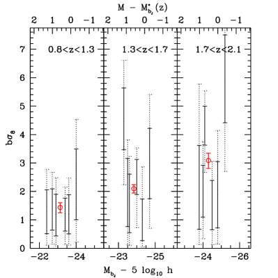
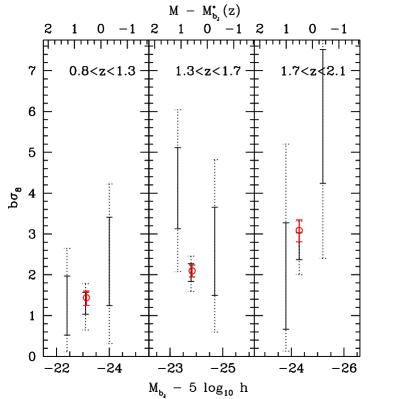
Figure 2: Left panel: $\sigma_{8}^{\rm q}$, i.e. $b\sigma_{8}$, as function of the median absolute magnitude for the low (left), medium (centre) and high (right) redshift bins. For each sample, the errorbars indicate the central 68.3 (solid) and 95.4 (dotted) credibility intervals of the marginalized bias probability distribution. On the upper axis, we indicate the magnitude difference with respect to M${}^{\star}_{b_{\rm J}}$(z), where the later is given by Eq. 13 of Croom et al. (2004). The open symbol show the result obtained by fitting the correlation function of all the quasars lying in this redshift bin (see PMN04). Right panel: Same as the left panel but for a three-parameter fit (see text).

4 Luminosity dependent clustering

In this section, we present the results obtained by fitting the auto- and cross-correlation functions presented in Fig. 1 with the model given in equation (4). Our aim is to quantify how the bias parameter of optically bright quasars depends on redshift and luminosity.

The best-fitting functions obtained with the Markov Chain Monte Carlo method are overplotted to the data in Fig. 1 (shaded regions). Note that, for all redshift bins, they accurately describe the quasar auto- and cross-correlations in the whole range of separations under analysis. In the left panel of Fig. 2, we plot $\sigma_{8}^{\rm q}$ (i.e. $b\sigma_{8}$) as a function of absolute magnitude. As expected, the bias parameter of all quasars lying in a given redshift bin (measured by PMN04 and represented with an open symbol) lies in between the values found here. Taken at face value, the data show some evidence for luminosity segregation; however, samples at different redshifts show different trends. The brightest quasars in the high-redshift bin seem to be more strongly clustered than the others. In the medium-redshift bin, the bias seems to follow a $U$-shape: the faintest and the brightest quasars in the set are typically more strongly clustered than M${}^{\star}_{b_{\rm J}}$ quasars. On the other hand, the low-redshift bin does not show any particular trend: the bias keeps constant with luminosity.

Note, however, that correlations between errorbars in Fig. 2 might create spurious trends with luminosity. Moreover, all the different sub-samples in a given redshift bin have consistent bias parameters at the $2\sigma$ level. Given these concerns, we want to use a robust statistical test to investigate whether our data show any sign of luminosity dependent clustering.

4.1 Does quasar clustering depend on luminosity?

If there is no luminosity segregation, all our data should be described by one single bias parameter (i.e. all the $b_{i}$ should assume the same identical value). If, instead, some luminosity bins show a statistically significant deviation from the overall clustering amplitude, then a description with a number of different bias parameters should be preferred. Therefore, in this section we address the issue of luminosity dependent clustering by answering the following question: how many bias parameters are required to adequately describe the quasar auto- and cross-correlations in a given redshift bin? In other words, we want to understand how many different bias parameters can be reliably measured in a statistically significant way. This is a classical problem of model selection where we want to find the proper tradeoff between goodness of fit (in the $\chi^{2}$ sense) and complexity (in terms of number of free parameters). We use five different methods: the F-test, the Akaike information criterion (AIC), the Bayes factors (BF), the Bayesian information criterion (BIC) and the deviance information criterion (DIC, see the Appendix for a brief review). We consider three different models. In the first one, there is no clustering segregation with luminosity and all the luminosity bins at a given redshift are associated with the same bias parameter. In the second model, we use three bias parameters (one each for the brightest, B25, and faintest samples, F25, and one for the remaining quasars: hereafter those samples are referred to as B, M and F, for bright, medium and faint). In the third model, each luminosity bin has its own bias parameter, as already described in the previous sections. In Fig. 2, we show that the results of the three- and six-parameters models are qualitatively and quantitatively similar.

Before comparing the different models, it is worth noticing that, based on the $\chi^{2}$ statistic, a single parameter fit gives an acceptable description of the data for all redshift bins. Of course, using additional parameters reduces the minimum $\chi^{2}$ of the best-fitting models. We want now to understand whether this $\chi^{2}_{\rm min}$ reduction is statistically significant.

Performing the $F$-test and using the 95 per cent confidence level as a threshold to prefer a model with respect to another, we find that the low-redshift sample is best-fitted by a one-parameter model, while the medium- and high-redshift samples are best described by a six-parameter model. Similarly, all the Bayesian and information-theory based tests mentioned above clearly indicate that the low-redshift sample is best described by a one-parameter model. On the other hand, for the medium- and high-redshift samples, the situation is more confused. Because of the different penalties for model-complexity, depending on the adopted test, either the six- or the one-parameter model is the preferred one. However, with the exception of the six-parameter fit with the Akaike criterion, no model can be rejected with high-confidence (see Table 2 for a summary of the results). Therefore, we conclude that, while there is no evidence of clustering segregation with luminosity in the low-redshift sample, we find marginal evidence for it in the medium- and high-redshift samples.

Table 2: Number of parameters of the preferred models according to various model-selection criteria. When the evidence for the best model is not strong, we list all the acceptable models (in order of decreasing evidence). We use a 95 per cent confidence level for the F-test, AIC and DIC while we discard models with substantial evidence according to the Kass-Raftery criterion (see Appendix) for BF and BIC.

Criterion	$0.8<z<1.3$	$1.3<z<1.7$	$1.7<z<2.1$
F-test	1	6	6
AIC	1-3	1-3	1-3
BF	1-3-6	6-3-1	6-3-1
BIC	1	1-3-6	1-3-6
DIC	1-3-6	6-3-1	6-3-1

Following a suggestion of the referee, we have also tried to combine data from the different redshift bins by using a simple parameterization of the luminosity and redshift dependent bias. For simplicity, we adopted a linear relation with quasar luminosity $b(M_{b_{\rm J}},z)=b_{0}(z)+b_{1}10^{-0.4(M_{b_{\rm J}}-M^{\star}_{b_{\rm J}}(z))}$. In this case, the $68.3$ per cent confidence interval for the luminosity-dependent parameter is $b_{1}=0.3^{+0.6}_{-0.7}$. This confirms that the evidence for clustering segregation with luminosity is marginal in our sample. Similar conclusions are drawn adopting quadratic or cubic relations for the luminosity dependence of the bias parameter. In all cases, the best-fitting model favours a larger bias parameter for the brightest quasars in our sample. However, the statistical significance of the result is low.

4.2 Limitations of the PCA method

A number of systematic effects can alter the model-fitting procedure (and thus the statistical significance of the results). In particular, for strongly correlated data, the choice of the number of principal components used in the fit plays a delicate role. We fixed $N_{\rm pca}$ assuming that our bootstrap errors are accurate estimates of the real uncertainties and using the $\chi^{2}$ test. Had we decided to include a few more components to account for 99 per cent of the variance (which is equivalent to consider 7 additional components for each redshift sample and still gives acceptable values of the reduced $\chi^{2}$), the evidence for clustering segregation would have been stronger. In Fig. 3 we compare the solutions for the three-parameter models obtained by minimizing $\chi^{2}_{95}$ (left) and $\chi^{2}_{99}$ (right). What is shown here are the (marginal) joint probability distributions of pairs of bias parameters (for the faint, medium and bright samples). Clustering segregation with luminosity is suggested by the data whenever the contours of the joint distributions lie away from the diagonal line. For both $\chi^{2}_{95}$ and $\chi^{2}_{99}$, this never happens for the low-redshift sample (the bottom-left set of curves) and the one-parameter solution has to be preferred. At best, clustering segregation with luminosity is detected at the $\sim 2\sigma$ level (for $\chi^{2}_{95}$) and at $\sim 3\sigma$ level (for $\chi^{2}_{99}$) in the high- and medium-redshift samples. Note that, even though a 3$\sigma$ detection is still consistent with pure statistical fluctuations, when $\chi^{2}_{99}$ is used, all the tests for model selection strongly prefer either the three- or the six-parameter solution with respect to the one-parameter fit. In other words, the results presented in the previous section have to be considered conservative. If one decides to use the full covariance matrix, one will infer the presence of a statistically significant clustering segregation with luminosity in the medium- and high-redshift samples. Hence, the uncertainty in the number of physical components is the main limitation of the principal component technique that we used to account for correlated errorbars. Bayesian techniques (e.g. Minka 2000) suggest that the components which contribute the last few per cent of the bootstrap variance are most likely dominated by noise. Therefore, we are confident that the results we presented in section 4.1 are optimal and realistic. Larger datasets with smaller intrinsic uncertainties are thus needed to improve the significance of our results.

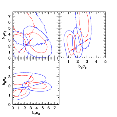
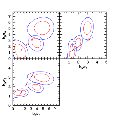
Figure 3: Left panel: Results obtained by fitting the data with a three-parameter model (see text) where $b_{\rm B}$, $b_{\rm M}$ and $b_{\rm F}$ are the bias parameters for the bright, medium and faint sub-samples (at fixed redshift), respectively. The contours indicate the 68.3 and 95.4 per cent credibility intervals for the (marginalized) joint probability distribution of two bias parameters. On the diagonal, we indicate the corresponding confidence levels for the one-parameter fits. The results for the low, medium and high redshif1t samples are plotted from left to right: $b\sigma_{8}$ clearly increases with redshift. Right panel: Same as left panel but using more principal components of the errors so as to account for 99 per cent of the variance (as opposed to 95 per cent in the left panel). Note that errorbars shrink and $b_{\rm F}$ is shifted by almost 1$\sigma$ with respect to the left panel.

In order to cross-check our results with a method affected by different systematics, we have computed the marked correlation function of the quasars (e.g. Sheth, Connolly & Skibba 2006 and references therein) using their blue luminosity as the mark. Results for the medium redshift sample are shown in Fig. 4. Here we define the marked correlation function (filled squares) as the ratio of the projected quasar correlation function weighted by the quasar luminosity (numerator) and the usual projected quasar correlation function (denominator). By construction, this ratio is not affected by redshift space distortions. The open symbols correspond to the mean marked correlation function obtained by averaging over one hundred realisations with randomized marks. To assess the significance of the marked statistics, one usually compares the signal with the standard deviation around the mean of the randomized realisations. From Fig. 4, we see that, on average, the closest quasar pairs have higher luminosities, thus suggesting the presence, on those scales, of some clustering segregation. However, given the size of the errorbars, the statistical significance of this trend is rather small. We note that the errors used here only reflect the uncertainty arising from the distribution of the marks and do not include any uncertainty in the actual estimate of the correlation function. Considering the corresponding bootstrap errors (which, for instance, allow for sample variance), the uncertainties on the marked correlation function typically increase by 20-30 per cent. This makes the detection of clustering segregation even more uncertain. In summary, the analysis of the marked statistics reaches exactly the same conclusions as our main work: even though there is some evidence for luminosity-dependent clustering in our high-redshift data, our sample is too small to provide a robust detection. Similar results are obtained for the other redshift bins.

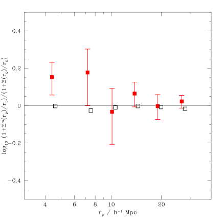
Figure 4: Marked correlation function of the medium redshift sample obtained using the blue luminosity of the quasars as the mark. The empty squares (that have been slightly displaced to the right) show the mean obtained by averaging over one hundred realizations of the same measurement after randomizing the marks. Errorbars show the standard deviation around this mean. If one includes bootstrap errors into the total error budget (not shown here), the errors on the marked correlation function typically increase by 20-30 per cent.

4.3 Discussion

When interpreting our results, we have to consider the limitations of both the dataset and the method used to extract the bias parameters. First, the depth of the quasar sample is such that at a given redshift we can only probe a factor of ten in luminosity. This implies that any luminosity segregation has to be observed over this relatively small luminosity range. By slicing the different redshift bins into six sub-samples, our analysis tries to extract the maximum possible information from these limited data. However, to avoid to be dominated by measurement noise, we compare narrow luminosity intervals (at both the bright and faint ends) with larger control samples. This naturally leads to the selection of partially overlapping luminosity ranges. For this reason, our samples, despite probing different absolute magnitude intervals, are not independent from each other. Note the striking difference from previous studies of galaxy clustering (see e.g. Norberg et al. 2001, 2002) where one can perform several independent measurements of the clustering amplitude as a function of luminosity and span a wide magnitude range.

Given these limitations and based on theoretical models of quasar clustering, should have we expected to detect some luminosity dependence in our dataset? As discussed in the introduction, models make very different predictions. From Fig. 3 in Lidz et al. (2006) we infer that the models which assume a tight correlation between quasar luminosity and the mass of the host-halos predict a difference $\Delta b=(b_{\rm B25}-b_{\rm F25})\,\sigma_{8}\sim 1$ for our high-redshift bin. On the other hand, models based on merger simulations predict $\Delta b\sim 0.2$. Similarly, the semi-analytic models by Kauffman & Haehnelt (2002) predict $0.3\mathrel{\hbox to0.0pt{\lower 3.0pt\hbox{$\sim$}\hss}\raise 2.0pt\hbox{$<$}}\Delta b\mathrel{\hbox to0.0pt{\lower 3.0pt\hbox{$\sim$}\hss}\raise 2.0pt\hbox{$<$}}0.7$ depending on the characteristic quasar lifetime (this increases up to $\Delta b\sim 1$ at $z\simeq 1.5$). In all cases, the errorbars associated with our measurements are too large to lead to a statistically significant detection of luminosity dependent clustering (in fact, our error on $\Delta b$ is $\sigma_{\Delta b}\simeq 2.3$ and we measure $\Delta b\simeq 4.3$ which is only $1.4\,\sigma$ and $1.8\,\sigma$ away from the two reference models). Assuming that $\Delta b\simeq 1$, a sample which is nearly fifty times larger than ours (i.e. nearly all-sky) is needed to detect the luminosity dependence at the $3\,\sigma$ confidence level (assuming that the error scales with the sample size, $n$, as $n^{-1/2}$). Very likely a sample of this size will not be available in the next few years. Alternatively, one could try to beat the noise by reaching a fainter apparent magnitude limit. Fig. 3 in Lidz et al. (2006) shows that current models predict that, by reducing the median luminosity of our F25 sample by a factor of 10, one would get $0.6\mathrel{\hbox to0.0pt{\lower 3.0pt\hbox{$\sim$}\hss}\raise 2.0pt\hbox{$<$}}\Delta b\mathrel{\hbox to0.0pt{\lower 3.0pt\hbox{$\sim$}\hss}\raise 2.0pt\hbox{$<$}}2$. Note that a value of $\Delta b\sim 2$ could be ruled out at the $3\,\sigma$ confidence level by using a sample twelve times as large as ours. In conclusion, our analysis can only rule out (or detect) extreme luminosity dependent biasing and future surveys are required to discriminate among current models.

Table 3: Best-fitting constant-bias (columns 4,5 and 6) and power-law models for six complementary redshift bins. The goodness of each fit is measured by the quantity $\chi^{2}_{\rm min}/{\rm dof}$ which gives the minimum value assumed by the $\chi^{2}$ statistic divided by the number of degrees of freedom.

$z_{\rm l}$	$z_{\rm h}$	$z_{\rm m}$	$b$	$r_{0}$	$\chi^{2}_{\rm min}/{\rm dof}$	$r_{0}$	$\gamma$	$\chi^{2}_{\rm min}/{\rm dof}$	$r_{0}^{(\gamma=1.8)}$	$\chi^{2}_{\rm min}/{\rm dof}$
				($\,h^{-1}\,{\rm Mpc}$)		($\,h^{-1}\,{\rm Mpc}$)			($\,h^{-1}\,{\rm Mpc}$)
0.80	1.06	0.933	$1.57^{+0.30}_{-0.37}$	$5.5^{+1.5}_{-1.8}$	$3.47/3$	$4.3^{+2.5}_{-4.2}$	$1.70^{+0.53}_{-0.67}$	$2.02/2$	$4.9^{+0.8}_{-1.1}$	$2.05/3$
1.06	1.30	$1.185$	$1.76^{+0.35}_{-0.43}$	$5.6^{+1.6}_{-1.9}$	$1.07/3$	$5.1^{+1.6}_{-4.3}$	$1.84^{+0.33}_{-0.68}$	$0.87/2$	$4.9^{+1.0}_{-1.2}$	$0.89/3$
1.30	1.51	$1.410$	$2.13^{+0.29}_{-0.33}$	$6.5^{+1.2}_{-1.3}$	$1.05/3$	$6.1^{+1.2}_{-2.1}$	$1.93^{+0.44}_{-0.42}$	$1.44/2$	$5.6^{+0.9}_{-0.9}$	$1.54/3$
1.51	1.70	$1.602$	$2.33^{+0.33}_{-0.39}$	$6.7^{+1.2}_{-1.5}$	$5.33/3$	$4.1^{+2.3}_{-3.9}$	$1.59^{+0.38}_{-0.55}$	$4.92/2$	$5.4^{+0.8}_{-0.9}$	$5.17/3$
1.70	1.89	$1.796$	$3.02^{+0.45}_{-0.53}$	$8.5^{+1.5}_{-1.9}$	$0.53/3$	$7.2^{+1.2}_{-2.7}$	$2.03^{+0.43}_{-0.47}$	$1.19/2$	$6.3^{+1.0}_{-1.3}$	$1.48/3$
1.89	2.10	$1.987$	$4.13^{+0.49}_{-0.55}$	$11.5^{+1.5}_{-1.7}$	$2.76/3$	$8.8^{+1.2}_{-4.9}$	$1.82^{+0.27}_{-0.49}$	$2.86/2$	$8.6^{+1.1}_{-1.2}$	$2.87/3$

5 Redshift-dependent clustering

In this section we focus on the redshift dependence of the quasar clustering amplitude. This is done in real space, using the projected correlation function. Our study is thus complementary to the redshift-space analysis by Croom et al. (2005) which might be affected by large-scale infall. In this section we also discuss the effect of using different methods for determining the quasar correlation length.

To improve the analysis performed by PMN04 and better study the evolution with cosmic time, we split our quasar sample into six redshift bins. These are obtained by dividing into two equal sized parts (in terms of quasar number) the redshift bins used in the previous sections and in PNM04. We first compute the projected auto-correlation functions of all the quasars which lie in a given redshift bin. We then use the method described in §3.2 to fit these data with the model given in equation (4). The best-fitting models correspond to very good values of the $\chi^{2}$ statistic, indicating that our models accurately describe the spatial dependence of the measured correlations. Finally, we estimate the correlation length, $r_{0}$, by determining the scale at which the best-fitting model has $\xi^{\rm q}(r)=1$. For comparison, we also fit a power-law model $\xi^{\rm q}(r)=(r/r_{0})^{\gamma}$. We distinguish two cases where we either allow both $r_{0}$ and $\gamma$ to vary or we fix $\gamma=1.8$. Our results are reported in Table 3 (together with the corresponding 68.3 per cent confidence levels) and plotted in Fig. 5. Note that the best-fitting values for the quasar correlation length derived from the power-law model are systematically lower than the CDM ones (the two estimates are anyway consistent within $1\sigma$ uncertainties). This is because, in a CDM model, the power-law index of the mass auto-correlation function is a function of the spatial separation. For instance, $\gamma_{\rm eff}=d\ln\xi/d\ln r\simeq 1.3$ at $r=5$ $\,h^{-1}\,{\rm Mpc}$, while $\gamma_{\rm eff}\simeq 1.9$ at $r=20$ $\,h^{-1}\,{\rm Mpc}$. Similarly, the projected correlation function, $\Xi(r_{\perp})/r_{\perp}$, has a slope varying between $1.6$ and 2.3 when $5<r<20$ $\,h^{-1}\,{\rm Mpc}$. Therefore, a CDM model has a much lower correlation on large-scales with respect to a power-law model with the same $r_{0}$ (and $\gamma<2$). It is then clear from equation (5) that a CDM model needs a higher overall normalization than a power-law model to fit the same projected correlation.

The evolution of the quasar correlation length between $0.8<z<2.1$ can be approximately described by the linear relation

$$r_{0}=\left[7.3+5.2\,(z-1.5)\right]h^{-1}\,{\rm Mpc}$$ (6)

(this becomes $r_{0}=[6.1+3.6\,(z-1.5)]$ $\,h^{-1}\,{\rm Mpc}$ for the values of $r_{0}$ determined with the power-law fit to $\Xi(r_{\perp})/r_{\perp}$). For $0.8<z<1.6$, our results are in good agreement with Croom et al. (2005), but we find evidence for a stronger variation at high-z (see Fig. 5). This is more evident when we use the CDM model to fit the data. The models by Kauffman & Haehnelt (2002) with a quasar lifetime of $\sim 10^{7}$ yr match our data at $z<1.7$. However, as already pointed out in PMN04, an increase in the lifetime by nearly an order of magnitude is required to reproduce the biased-CDM fits at $z\sim 2$.

Given that the mass autocorrelation function rapidly increases with cosmic time, the bias parameter of our quasars has to increase with $z$. The bottom panel of Fig. 5 shows the evolution of $b$. Note that, within the range of cosmological models allowed by observations, the quasar bias parameter scales linearly with $\sigma_{8}$. For this reason we decided to plot the product $\sigma_{8}^{\rm q}=b\,\sigma_{8}$ which is independent on the assumed value for the amplitude of the linear power spectrum. Similarly to the correlation length, $\sigma_{8}^{\rm q}$ seems to increase rapidly for $z>1.6$ and the bias evolution is well approximated by the relation

$$b\sigma_{8}=1+\left(\frac{1+z}{2.5}\right)^{5}\;.$$ (7)

In CDM models, the clustering amplitude of massive dark-matter halos mainly depends on their mass. It is then interesting to see what halo masses correspond to the bias parameters of the 2QZ quasars. In the bottom panel of Fig. 5, we plot the evolution of $\sigma_{8}^{q}$ for a number halo masses which is obtained using the model by Sheth & Tormen (1999). The observed bias evolution is well reproduced by assuming that quasars are associated with halos of mass $\sim 10^{13}M_{\odot}$. This is fully consistent with the more detailed analysis performed in PMN04.

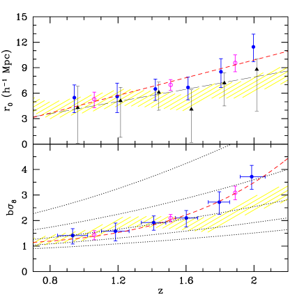
Figure 5: Top: Redshift evolution of the quasar correlation length. Filled circles with errorbars indicate the best-fitting values obtained using a biased CDM model. The short-dashed line is the analytical fit to the data given in equation (6). Filled triangles with errorbars refer to the best-fitting values obtained with a power-law model (where both $\gamma$ and $r_{0}$ are free to vary). These points have been slightly displaced to the right to improve readibility. The long-dashed line is the linear fit to the data given in the main text. Empty symbols are analogous to their filled counterparts but are obtained using larger redshift intervals as in PMN04. The shaded area marks the 68.3 confidence levels obtained by Croom et al. (2005). Bottom: As in the top panel but for the quasar bias parameter. Horizontal errorbars mark the $16^{\rm th}$ and the $68^{\rm th}$ percentiles of the redshift distribution in a bin. The dashed line is the fitting function given in equation (7). The dotted lines indicate the bias evolution for dark matter halos with masses $10^{12},10^{12.5},10^{13},10^{13.5}$ and $10^{14}M_{\odot}$ (from bottom to top).

6 Summary

We have used a flux limited sample of $\sim 14,000$ 2QZ quasars brighter than M${}_{\rm b_{\rm J}}-5\log_{10}h=-21.7$ to study the quasar clustering properties in the redshift range $0.8<z<2.1$. Our main results are summarized as follows.

(i) Splitting the sample in three redshift intervals each divided into six luminosity ranges and combining information from the corresponding auto- and cross-correlation functions, we find some evidence for clustering segregation with luminosity. For redshifts $z>1.3$, a frequentist model selection technique (the F-test) prefers a multi-parameter fit to the data at the 95 per cent confidence level

(ii) A number of statistical tests based on information theory and Bayesian techniques show weak evidence for luminosity dependent clustering at high redshift ($z>1.3$) and no evidence at low redshift ($z<1.3$). These results somewhat depend on the number of principal components used in the fitting procedure. Accounting for a larger fraction of the bootstrap variance increases the significance of the detection of clustering segregation with luminosity.

(iii) Larger datasets, possibly with a deeper coverage, are needed to discriminate among current models of quasar formation and to pin-point the detailed quasar clustering trends as a function of luminosity at a given redshift.

(iv) Splitting the sample into six complementary redshift bins, we find strong evidence for an increase of the clustering amplitude with lookback time. We detect pure quasar-clustering evolution between $z_{\rm eff}=0.93$ and $z_{\rm eff}=1.99$ at the $2.7\sigma$ confidence level. A linear fit for the evolution of $r_{0}$ with redshift is given in equation (6).

(v) Accounting for the evolution of the mass density in a $\Lambda$CDM model, we find that the high-redshift quasars ($z_{\rm eff}=1.99$) are $\sim 2.6$ times more biased than their low-redshift counterparts ($z_{\rm eff}=0.93$). Evolution in $b$ is detected at the $4.3\sigma$ confidence level.

(vi) The clustering amplitude of optically selected quasars suggests that they are hosted by halos with mass $M\sim 10^{13}M_{\odot}$ (see also PMN04).

Appendix A Model selection criteria

The F-test. If the uncertainties of the measurements are known to a good precision, model selection can be performed using a simple $\chi^{2}$ test. However, we cannot prove that our bootstrap errors accurately reproduce the true scatter in the data. An alternate test that does not require knowledge of the true standard deviation (up to a constant scaling factor) is to form the ratio

$${\cal F}=\frac{\chi^{2}_{n-k}-\chi^{2}_{n}}{k}\frac{N-n}{\chi^{2}_{n}}$$ (8)

where $N$ is the number of independent data values used in the fit (in our case $N=N_{\rm pca}$). The numerator in this equation is the difference between the $\chi^{2}$ calculated for $n$ parameters and that for $n-k$ parameters. Being a ratio of two $\chi^{2}$-distributed variables, ${\cal F}$ follows an $F$-distribution with $(k,N-n)$ degrees of freedom. We can then estimate how significant is the addition of $k$ parameters by integrating this distribution from 0 to ${\cal F}$.

The Akaike information criterion. The question to find which model best approximate a given dataset can be addressed in terms of information theory: the best model minimizes the loss of information. The Akaike information criterion (AIC) evaluates models using the Kullback-Leibler information (Akaike 1973). In terms of the number of independent datapoints, $n$, and of model parameters, $p$,

$${\rm AIC}=\chi^{2}_{\rm min}+2p+\frac{2p\,(p+1)}{n-p-1}$$ (9)

where the second order term on the right is needed when the size of the dataset does not exceed the number of model parameters by a large factor ($\mathrel{\hbox to0.0pt{\lower 3.0pt\hbox{$\sim$}\hss}\raise 2.0pt\hbox{$>$}}40$). The model with the minimum AIC has to be considered the best. Note that the AIC penalizes for the addition of parameters and thus selects a model that fits well but has a minimum number of parameters. The relative probability that a model is the correct solution is given by the Akaike weights

$$w_{i}=\frac{e^{-\Delta{\rm AIC}_{i}/2}}{\sum_{k=1}^{N}e^{-\Delta{\rm AIC}_{k}/2}}$$ (10)

where the indices $i$ and $k$ run over the different models and $\Delta{\rm AIC}={\rm AIC}_{i}-\min_{k}({\rm AIC}_{k})$. In general, models receiving AIC within 2 of the “best” deserve consideration, those within 3-7 have considerably less support and those above 7 are basically rejected by the test (Burnham & Anderson 1998).

The Bayes factor. Bayes factors are the dominant method for Bayesian model testing (see Kass & Raftery 1994 for an extensive review). The Bayes factor, $B_{12}$, is the ratio between the marginalized likelihoods (i.e. between the probabilities of the data given the models) for two different models (1 and 2) and provides a scale of evidence in favour of a model versus another. The model with the highest marginalized likelihood is the best. Following an early suggestion by Jeffreys (1961), Kass & Raftery (1994) proposed the following “rule of thumb” for interpreting the Bayes factors: $1<B_{12}<3$ provides weak evidence (barely worth mentioning) for model 1, $3<B_{12}<12$ provides substantial evidence for model 1, $12<B_{12}<150$ provides strong evidence for model 1, $B_{12}>150$ provides decisive evidence for model 1. Several numerical approaches have been proposed to compute Bayes factors based on MCMC sampling but most of these methods are subject to numerical or stability problems (see e.g. Han & Carling 2000 for a review). As a compromise between accuracy and coding complexity we estimate the Bayes factors using the harmonic mean estimator (see e.g. Kass & Raftery 1994). We repeat the calculation using three different chains and we use the standard deviation among them as an estimate of the uncertainty of our marginalized likelihoods.

The Bayesian information criterion. Unfortunately, while Bayes Factors are rather intuitive, as a matter of fact they are often quite difficult to calculate. This makes simpler (but approximate) estimates of the Bayes factors of great interest. Schwarz (1978) derived the Bayesian information criterion (BIC) as a large sample approximation to twice the logarithm of the Bayes factor.

$${\rm BIC}_{1}-{\rm BIC}_{2}\simeq-2\ln(B_{12})\;,$$ (11)

with

$${\rm BIC}=\chi^{2}_{\rm min}+p\,\ln n\;.$$ (12)

Similarly to the AIC, the preferred model is the one with the lowest value of the criterion. The Kass-Raftery criterion for model selection is also applied to the BIC.

The Deviance Information Criterion. Spiegelhalter et al. (2002) have recently proposed a Bayesian generalization of the AIC: the deviance information criterion (DIC). It is based on the posterior distibution of the log-likelihood or deviance ($D=-2\log{\cal L}$ which, in our case, coincides with $\chi^{2}$ function):

$${\rm DIC}=\langle D\rangle+p_{D}$$ (13)

where $\langle D\rangle$ is the posterior expectation of the deviance while the effective number of parameters, $p_{D}$, is defined as the difference between the posterior mean of the deviance and the deviance evaluated at the posterior mean of the parameters. $p_{D}=\langle D\rangle-D(\langle\theta\rangle)$. The DIC can be re-written as

$${\rm DIC}=D(\langle\theta\rangle)+2p_{D}$$ (14)

which makes the analogy with the first-order AIC explicit. A good model corresponds to a low DIC and model-selection criteria developed for the AIC appear to work well also for the DIC (Spiegelhalter et al. 2002). Note, however, that, since $p_{D}\leq p$, the DIC tends to be less conservative than the AIC in terms of model complexity. The main attraction of using this measure is that it is trivial to compute when performing MCMC on the models.

References

- [Adelberger & Steidel(2005)] Adelberger, K. L., & Steidel, C. C. 2005, ApJL, 627, L1
- [] Akaike, H. 1973, Information theory and Extension of the Maximum Likelihood Principle, in Second International Symposium on Information Theory, eds. B. N. Petrox and F. Caski, Budapest, Akademiai Kiado, pp. 267
- [] Burnham, K. P., & Anderson, D. R., 1998, Model Selection and Inference: a Practical Information-theoretic approach, New York, Springer
- [Croom et al.(2002)] Croom, S. M., Boyle, B. J., Loaring, N. S., Miller, L., Outram, P. J., Shanks, T., & Smith, R. J. 2002, MNRAS, 335, 459
- [Croom et al.(2004)] Croom, S. M., Smith, R. J., Boyle, B. J., Shanks, T., Miller, L., Outram, P. J., & Loaring, N. S. 2004, MNRAS, 349, 1397
- [Croom et al.(2005)] Croom, S. M., et al. 2005, MNRAS, 356, 415
- [FerrMerr (2000)] Ferrarese, L., & Merritt, D. 2000, ApJL, 539, L9
- [] Han, C.,& Carling, B. P. 2000, MCMC methods for computing Bayes factors: a comparative review, Working paper, Division of Biostatistics, School of Public Health, University of Minnesota
- [] Jeffreys, H. 1961, Theory of probability, Third edition, Oxford Univ. Press
- [Hopkins et al. (2005)] Hopkins, P.F., Hernquist, L., Cox T.J., Di Matteo, T., Robertson, B., Springel V. 2005, ApJ in press, astro-ph/0504252
- [] Kass, A. E., & Raftery, R. E. 1994, Technical Report no. 254, Dept. of Statistics, Univ. of Washington, Technical Report no. 571, Dept. of Statistics, Carnegie-Mellon University
- [Kauffmann & Haehnelt(2000)] Kauffmann, G., & Haehnelt, M. 2000, MNRAS, 311, 576
- [Kauffmann & Haehnelt(2002)] Kauffmann, G., & Haehnelt, M. 2002, MNRAS, 332, 529
- [Lidz et al. (2006)] Lidz, A., Hopkins, P.F., Cox, T.J., Hernquist, L. & Robertson, B. 2006, ApJ, 641, 41
- [] Minka, T. P. 2000, Automatic choice of dimensionality for PCA, M.I.T. Media Laboratory Perceptual Computing Section Technical Report No. 514
- [Norberg et al.(2001)] Norberg, P., et al. 2001, MNRAS, 328, 64
- [Norberg et al.(2002)] Norberg, P., et al. 2002, MNRAS, 332, 827
- [Porci 2002] Porciani C. & Giavalisco M., 2002, ApJ, 565, 24
- [Porciani et al.(2004)] Porciani, C., Magliocchetti, M., & Norberg, P. 2004, MNRAS, 355, 1010
- [Schwarz(1978)] Schwarz, G. 1978, Annals of Statistics, 6, 461
- [Shetetal)] Sheth, R. K., Connolly, A. J., Skibba, R., 2006, MNRAS submitted, astro-ph/0511773
- [] Spiegelhalter, D. J., Best, N. G., Carlin, B. P., & van der Linde, A. 2002, J.R. Statist. Soc. B, 64, Part 4, 583
- [Springel et al.(2005)] Springel, V., Di Matteo, T., & Hernquist, L. 2005, MNRAS, 623
- [Volonteri et al.(2003)] Volonteri, M., Haardt, F., & Madau, P. 2003, ApJ, 582, 559
- [Wyithe & Loeb(2003)] Wyithe, J. S. B., & Loeb, A. 2003, ApJ, 595, 614