Global structures in a composite system of two
scale-free discs with a coplanar magnetic field

Abstract

We investigate a theoretical magnetohydrodynamic (MHD) disc problem involving a composite disc system of gravitationally coupled stellar and gaseous discs with a coplanar magnetic field in the presence of an axisymmetric dark matter halo. The two discs are expediently approximated as razor-thin, with a barotropic equation of state, a power-law surface mass density, a ring-like magnetic field, and a power-law rotation curve in radius $r$. By imposing the scale-free condition, we construct analytically stationary global MHD perturbation configurations for both aligned and logarithmic spiral patterns using our composite MHD disc model. MHD perturbation configurations in a composite system of partial discs in the presence of an axisymmetric dark matter halo are also considered. Our study generalizes the previous analyses of Lou & Shen and Shen & Lou on the unmagnetized composite system of two gravitationally coupled isothermal and scale-free discs, of Lou and Shen et al. on the cases of a single coplanarly magnetized isothermal and scale-free disc, and of Lou & Zou on magnetized two coupled singular isothermal discs. We derive analytically the stationary MHD dispersion relations for both aligned and unaligned perturbation structures and analyze the corresponding phase relationships between surface mass densities and the magnetic field. Compared with earlier results, we obtain three solution branches corresponding to super fast MHD density waves (sFMDWs), fast MHD density waves (FMDWs) and slow MHD density waves (SMDWs), respectively. We examine the $m=0$ cases for both aligned and unaligned MHD perturbations. By evaluating the unaligned $m=0$ case, we determine the marginal stability curves where the two unstable regimes corresponding to Jeans collapse instability and ring fragmentation instability are identified. We find that the aligned $m=0$ case is simply the limit of the unaligned $m=0$ case with the radial wavenumber $\xi\rightarrow 0$ (i.e., the breathing mode) which does not merely represent a rescaling of the equilibrium state. We further show that a composite system of partial discs behaves much differently from a composite system of full discs in certain aspects. We provide numerical examples by varying dimensionless parameters $\beta$ (rotation velocity index), $\eta$ (ratio of effective sound speed of the two discs), $\delta$ (ratio of surface mass density of the two discs), $q$ (a measure of coplanar magnetic field strength), $F$ (gravity potential ratio), $\xi$ (radial wavenumber). Our formalism provides a useful theoretical framework in the study of stationary global perturbation configurations for MHD disc galaxies with bars, spirals and barred spirals.

1 Introduction

The large-scale structure of disc galaxies has long been studied observationally and theoretically by astrophysicists from various complementary aspects. Lin & Shu (1964, 1966) and their co-workers pioneered the classic density wave theory and achieved a great success in understanding the dynamical nature of spiral galaxies (Lin, 1987; Binney & Tremaine, 1987; Bertin & Lin, 1996). The basic idea of analyzing such a large-scale density wave problem is to treat coplanar perturbations in a background axisymmetric rotating disc; this procedure has been proven to be powerful in probing the galactic dynamics to various extents. In such a model development, perturbations (either linear or nonlinear) are introduced onto a background equilibrium to form local or large-scale structures and to perform stability analysis under various situations. Broadly speaking, axisymmetric and non-axisymmetric perturbations may lead to aligned configurations while non-axisymmetric perturbations can naturally produce spiral wave patterns. Theoretically, a disc system may be treated as razor-thin for simplicity (Syer & Tremaine, 1996; Shen & Lou, 2004b; Lou & Zou, 2004; Shen et al., 2005), with a mass density $\rho=\Sigma(r,\theta)\delta(z)$ under the situation where the thickness of a galactic disc is sufficiently small compared with its radial size scale; in this manner, the model problem reduces to a two-dimensional one.

In theoretical model investigations, two classes of disc models are frequently encountered. One class is the so-called singular isothermal discs (SIDs), which bears a flat rotation curve and a constant ‘temperature’ with a diverging surface mass density towards the centre [e.g., Shu et al. (2000)]. Since the early study by Mestel (1963) more than four decades ago, this idealized theoretical SID model has attracted considerable interest among astrophysicists in various contexts of disc dynamics [e.g., Zang (1976); Toomre (1977); Lemos et al. (1991); Goodman & Evans (1999); Shu et al. (2000); Lou (2002); Lou & Fan (2002); Lou & Shen (2003); Lou & Zou (2004); Lou & Wu (2005); Lou & Zou (2006)]. The other class is the so called scale-free discs [e.g. Syer & Tremaine (1996); Shen & Lou (2004b); Shen et al. (2005); Wu & Lou (2006)] and is the main focus of this paper. Being of a more general form for differentially rotating discs, a scale-free disc has a rotation curve in the form of $v\propto r^{-\beta}$ (the case of $\beta=0$ corresponds to a flat rotation curve) and a barotropic equation of state in the form of $\Pi=K\Sigma^{n}$ where $\Pi$ is the vertically integrated two-dimensional pressure. There is no characteristic spatial scale and all quantities in the disc system vary as powers of radius $r$. In our analysis, the rotation velocity index $\beta$ satisfies $-1/4<\beta<1/2$ for warm discs. Furthermore, it is possible to construct stationary (i.e. $\omega=0$) density wave patterns in scale-free discs (Syer & Tremaine, 1996; Shen & Lou, 2004b; Shen et al., 2005; Wu & Lou, 2006), clearly indicating that the pattern speed of a density wave is in the opposite sense of the disc rotation speed.

Because of the self-gravity, one important technical aspect in dealing with thin disc galaxies involves the Poisson integral, relating the mass density distribution and gravitational potential. In the early development of the density wave theory, this Poisson integral is evaluated by an asymptotic analysis valid in the large wavenumber regime of the Wentzel-Kramers-Brillouin-Jeffreys (WKBJ) approximation. Based on this, the pursuit of analytical solutions leads to a further exploration of the problem. Several potential-density pairs are generalized in Chapter 2 of Binney & Tremaine (1987). One special utility is the logarithmic spiral potential-density pair first derived by Kalnajs (1971). This is a powerful tool in analyzing non-axisymmetric perturbations in an axisymmetric background disc. Furthermore, Qian (1992) made use of the techniques of Lynden-Bell (1989) and found a larger family of potential-density pairs in terms of the generalized hypergeometric functions. Using these results for scale-free discs under our consideration, the Poisson integral is solved analytically for both aligned and spiral perturbations (Shen & Lou, 2004b; Shen et al., 2005; Wu & Lou, 2006).

Magnetic field is an important ingredient in various astrophysical disc systems. In the interstellar medium (ISM), the partially or fully ionized gases make the cosmic space an ideal place for applying the magnetohydrodynamics (MHD) equations. In many astrophysical situations involving large-scale dynamics, the magnetic field can be effectively considered as completely frozen into the gas. While in some cases the magnetic force is relatively weak and has little impact on the dynamical process. There do exist certain situations when the magnetic field plays a crucial role in both dynamics and diagnostics, such as in spiral galaxies and accretion processes [e.g. Balbus & Hawley (1998); Balbus (2003); Fan & Lou (1996, 1997); Shu et al. (2000); Lou & Fan (1998a); Lou (2002); Lou & Fan (2003); Lou & Zou (2004, 2006); Shen et al. (2005); Lou & Wu (2005) ]. In terms of MHD model development, we need to prescribe the magnetic field geometry. Shu & Li (1997) introduced a model in which a disc is ‘isopedically’ magnetized such that the mass-to-flux ratio remains spatially uniform and the effect of magnetic field is subsumed into two parameters (Shu & Li, 1997; Shu et al., 2000; Lou & Wu, 2005; Wu & Lou, 2006). In fact, Lou & Wu (2005) have shown explicitly that a constant mass-to-flux ratio is a natural consequence of the frozen-in condition from the ideal MHD equations. In parallel, the coplanar magnetic field also serves as an interesting model (Lou, 2002; Lou & Zou, 2004; Shen et al., 2005) with the magnetic field being azimuthally embedded into the disc system. In particular, with the inclusion of an azimuthal magnetic field, one can construct the so-called fast and slow MHD density waves (FMDWs and SMDWs) (Fan & Lou, 1996, 1997; Lou & Fan, 1998a; Lou, 2002) and the interlaced optical and magnetic spiral arms in the nearby spiral galaxy NGC 6946 are sensibly explained along this line.

The stability of such MHD discs is yet another lively debated issue. In the WKBJ or tight-winding regime, the well-known $Q$ parameter criterion (Safronov, 1960; Toomre, 1964) was suggested to determine the galactic local axisymmetric stability in the absence of magnetic field. Meanwhile, there have been numerous studies concerning the global stability of the disc problem [e.g., Zang (1976); Toomre (1977); Lemos et al. (1991); Evans & Read (1998a, b); Goodman & Evans (1999); Shu et al. (2000)]. For example, stationary perturbations of the zero-frequency neutral modes are emphasized as the marginal instability modes in scale-free discs. In this context, Syer & Tremaine (1996) made a breakthrough in obtaining semi-analytic solutions for stationary perturbation configurations in a class of scale-free discs. Shu et al. (2000) analyzed the stability of isopedically magnetized SIDs and derived stationary perturbation solutions. They interpreted these aligned and unaligned configurations as onsets of bar-like instabilities. Lou (2002) performed a coplanar MHD perturbation analysis on azimuthally magnetized SIDs from a perspective of stationary FMDWs and SMDWs.

Our analysis on two-dimensional coplanar MHD perturbations has avoided at least two major issues. If perturbation velocity and magnetic field components perpendicular to the disc plane are allowed, it is then possible to describe Alfvénic fluctuations and model disc warping process. If one further takes into account of vertical variations across the disc (i.e., the disc thickness is not negligible), magneto-rotational instabilities can develop (e.g., Balbus 2003). These two aspects are important and should bear physical consequences in modelling disc galaxies.

In a typical disc galaxy system, the basic component involves stars, gases, dusts, cosmic rays, and a massive dark matter halo (Lou & Fan, 1998a, 2003). In terms of theoretical analysis, it would be a great challenge to include all these factors into one single model consideration. While limited in certain aspects, it remains sufficiently challenging and interesting to consider a composite system consisting of a coplanarly magnetized gas disc, a stellar disc as well as an axisymmetric background of a massive dark matter halo. A seminal analysis concerning a composite disc system dates back to Lin & Shu (1966, 1968) who combined a stellar distribution function and a gas fluid description to derive a local dispersion relation for galactic spiral density waves in the WKBJ approximation. Since then, there have been extensive theoretical studies on perturbation configurations and stability problems of the composite disc system. Jog & Solomon (1984a, b) investigated the growth of local axisymmetric perturbations in a composite stellar and gaseous disc system. Bertin & Romeo (1988) considered the spiral modes containing gas in a two-fluid model. Vandervoort (1991a, b) studied the effect of interstellar gas on oscillations and the stability of spheroidal galaxies. Romeo (1992) considered the stability of two-component fluid discs with finite thickness. Two-fluid approach was adopted into modal analysis morphologies of spiral galaxies by Lowe et al. (1994), supporting the notion that spiral structures are long-lasting and slowly evolving. Elmegreen (1995) and Jog (1996) suggested an effective $Q_{eff}$ (or $Q_{s-g}$) parameter criterion (Safronov, 1960; Toomre, 1964) for local axisymmetric two-fluid instabilities of a disc galaxy. Lou & Fan (1998b) explored basic properties of open and tight spiral density-waves modes in a two-fluid model to describe a composite system of coupled stellar and gaseous discs. Recently, Lou & Shen (2003) studied a composite SID system to derive stationary global perturbation configurations and further explored the axisymmetric instability properties (Shen & Lou, 2003) where they proposed a fairly straightforward $D$ criterion for the axisymmetric instability problem for a composite SID system. Shen & Lou (2004b) extended these analysis to a composite system of two scale-free discs and carried out analytical analysis on both aligned and logarithmic spiral perturbation configurations. By adding a coplanar magnetic field to the background composite SIDs, Lou & Zou (2004) obtained MHD perturbation configurations and further studied the axisymmetric instability problem (Lou & Zou, 2006).

The main objective of this paper is to construct global scale-free stationary configurations in a two-fluid gaseous and stellar disc system with an embedded coplanar magnetic field in the gas disc. Meanwhile, an axisymmetric instability analysis is also performed. There are several new features compared with previous works (Lou & Zou, 2004; Shen & Lou, 2004b; Shen et al., 2005) that may provide certain new clues to understand large-scale structures of disc galaxies. This paper is structured as follows. In Section 2, we present the theoretical formalism of the problem; both the stationary equilibrium state and the linearized MHD perturbation equations are summarized. In Section 3, we perform numerical calculations for the aligned perturbation configurations. Both the dispersion relation and phase relationship between density and the magnetic field perturbations are deduced and evaluated. In Section 4, we apply the same procedure to the analysis of global logarithmic spiral configurations. The $m=0$ marginal stability is also discussed. Finally, we summarize and discuss our results in Section 5. Several technical details are included in Appendices A, B, and C.

2 Fluid-Magnetofluid Discs

We adopt the fluid-magnetofluid formalism in this paper to construct large-scale stationary aligned and unaligned coplanar MHD disturbances in a background MHD rotational equilibrium of axisymmetry [Lou & Shen (2003); Lou & Zou (2004); Shen & Lou (2004b); Lou & Wu (2005); Lou & Zou (2006); Wu & Lou (2006)]. All the background physical quantities are assumed to be axisymmetric and to scale as power laws in radius $r$. Specifically, the rotation curves bear an index of $-\beta$ (viz., $\emph{v}\propto\emph{r}^{-\beta}$) and the vertically integrated mass density has the form $\Sigma_{0}\propto\emph{r}^{-\alpha}$ with $-\alpha$ being another index. Physically, the magnetofluid formalism is directly applicable to the magnetized gas disc, while the fluid formalism is only an approximation when applied to the stellar disc, where a distribution function approach would give a more comprehensive description. For our purpose of modelling large-scale stationary MHD perturbation structures and for mathematical simplicity, as well as the similarity between the two sorts of descriptions (Shen & Lou, 2004b), it suffices to work with the fluid-magnetofluid formalism.

In this section, we present basic MHD equations of the fluid-magnetofluid description for a composite system consisting of a scale-free stellar disc and a coplanarly magnetized gas disc. In our approach, the two gravitationally coupled discs are treated using the razor-thin approximation (i.e., we use vertically integrated fluid-magnetofluid equations and neglect vertical derivatives of physical variables along $z$) and the two-dimensional barotropic equation of state to construct global MHD perturbation structures. A coplanar magnetic field is involved in the dynamics of the thin gas disc following the basic MHD equations. The background state of axisymmetric rotational equilibrium is first derived. We then superpose coplanar MHD perturbations onto the equilibrium state and obtain linearized equations for MHD perturbations in the composite disc system.

2.1 Ideal Nonlinear MHD Equations

By our conventions, we use either subscript or superscript ‘$s$’ and ‘$g$’ to denote physical variables in association with the stellar disc and the magnetized gas disc, respectively. For large-scale MHD perturbations of our interest at this stage, all diffusive effects such as viscosity, resistivity, thermal conduction, and radiative losses etc. are ignored for simplicity. In cylindrical coordinates (r, $\theta$, z) and coincident with the z=0 plane, we readily write down the basic nonlinear ideal MHD equations for the composite disc system, namely

$${\partial{\Sigma^{g}}\over{\partial{t}}}+{1\over{r}}{\partial{}\over{\partial{r}}}{(r\Sigma^{g}u^{g})}+{1\over{r^{2}}}{\partial{}\over{\partial{\theta}}}{(\Sigma^{g}j^{g})}=0\ ,$$ (1)

$$\begin{split}{\partial{u^{g}}\over{\partial{t}}}+{u^{g}}{\partial{u^{g}}\over{\partial{r}}}+{{j^{g}}\over{r^{2}}}{\partial{u^{g}}\over{\partial{\theta}}}-{(j^{g})^{2}\over{r^{3}}}=-{1\over{\Sigma^{g}}}{\partial{\Pi^{g}}\over{\partial{r}}}-{\partial{\phi}\over{\partial{r}}}&\\ -{1\over{\Sigma^{g}}}\int{{\emph{d}zB_{\theta}\over{4\pi r}}\bigg{[}{\partial{(rB_{\theta})}\over{\partial{r}}}-{\partial{B_{r}}\over{\partial{\theta}}}\bigg{]}}\ ,\end{split}$$ (2)

$$\begin{split}{\partial{j^{g}}\over{\partial{t}}}+{u^{g}}{\partial{j^{g}}\over{\partial{r}}}+{{j^{g}}\over{r^{2}}}{\partial{j^{g}}\over{\partial{\theta}}}=-{1\over{\Sigma^{g}}}{\partial{\Pi^{g}}\over{\partial{\theta}}}-{\partial{\phi}\over{\partial{\theta}}}\qquad&\\ \qquad\qquad\qquad+{1\over{\Sigma^{g}}}\int{{\emph{d}zB_{r}\over{4\pi}}\bigg{[}{\partial{(rB_{\theta})}\over{\partial{r}}}-{\partial{B_{r}}\over{\partial{\theta}}}\bigg{]}}\ \end{split}$$ (3)

for the magnetized gas disc, and

$${\partial{\Sigma^{s}}\over{\partial{t}}}+{1\over{r}}{\partial{}\over{\partial{r}}}{(r\Sigma^{s}u^{s})}+{1\over{r^{2}}}{\partial{}\over{\partial{\theta}}}{(\Sigma^{s}j^{s})}=0\ ,$$ (4)

$${\partial{u^{s}}\over{\partial{t}}}+{u^{s}}{\partial{u^{s}}\over{\partial{r}}}+{{j^{s}}\over{r^{2}}}{\partial{u^{s}}\over{\partial{\theta}}}-{(j^{s})^{2}\over{r^{3}}}=-{1\over{\Sigma^{s}}}{\partial{\Pi^{s}}\over{\partial{r}}}-{\partial{\phi}\over{\partial{r}}}\ ,$$ (5)

$${\partial{j^{s}}\over{\partial{t}}}+{u^{s}}{\partial{j^{s}}\over{\partial{r}}}+{{j^{s}}\over{r^{2}}}{\partial{j^{s}}\over{\partial{\theta}}}=-{1\over{\Sigma^{s}}}{\partial{\Pi^{s}}\over{\partial{\theta}}}-{\partial{\phi}\over{\partial{\theta}}}$$ (6)

for the stellar disc in the ‘fluid’ approximation, respectively. Here, $\Sigma$ denotes the surface mass density, $u$ is the radial component of the bulk flow velocity, $j\equiv rv$ is the specific angular momentum in the vertical $z$-direction and $v$ is the azimuthal bulk flow velocity, $\Pi$ is the vertically integrated two-dimensional pressure, $B_{r}$ and $B_{\theta}$ are the radial and azimuthal components of the coplanar magnetic field $\textbf{\emph{B}}\equiv(B_{r},\ B_{\theta},\ 0)$, and $\phi$ is the total gravitational potential. This $\phi$ can be expressed in terms of the Poisson integral

$$\emph{F}\phi(r,\theta)=\oint{\emph{d}\varphi}\int_{0}^{\infty}{-G{\Sigma(r^{\prime},\ \varphi,\ t)r^{\prime}\emph{d}r^{\prime}}\over{[r^{\prime 2}+r^{2}-2r^{\prime}r\cos(\varphi-\theta)]^{1/2}}}\ ,$$ (7)

where $G$ is the gravitational constant, $\Sigma=\Sigma^{g}+\Sigma^{s}$ denotes the total surface mass density, and $F$ is defined as the ratio of the gravitational potential arising from the composite discs to that arising from the entire system including an axisymmetric massive dark matter halo that is presumed not to respond to the coplanar MHD perturbations in the disc plane [Syer & Tremaine (1996); Shu et al. (2000); Lou & Shen (2003); Lou & Zou (2004); Shen & Lou (2004b); Lou & Wu (2006); Lou & Zou (2006)] with $F=1$ for a full composite disc system and $0<F<1$ for a composite system of partial discs.

For a coplanar magnetic field $\textbf{\emph{B}}=(B_{r},B_{\theta},0)$ in cylindrical coordinates $(r,\theta,z)$, the divergence-free condition is

$${\partial{(rB_{r})}\over{\partial{r}}}+{\partial{B_{\theta}}\over{\partial{\theta}}}=0\ .$$ (8)

The radial and azimuthal components of the magnetic induction equation are

$${\partial{B_{r}}\over{\partial{t}}}={1\over{r}}{\partial{}\over{\partial{\theta}}}(u^{g}B_{\theta}-v^{g}B_{r})\ ,$$ (9)

$${\partial{B_{\theta}}\over{\partial{t}}}=-{\partial{}\over{\partial{r}}}(u^{g}B_{\theta}-v^{g}B_{r})\ .$$ (10)

Among $(\ref{eq:8})-(\ref{eq:10})$, only two of them are independent. The barotropic equation of state for the scale-free discs is

$$\Pi^{i}=K_{i}\Sigma^{n_{i}}\ ,$$ (11)

where $K_{i}>0$ is a constant proportional coefficient and $n_{i}>0$ is the barotropic index with subscript $i$ denoting either $g$ or $s$ for the two discs (we use this convention for simplicity). An isothermal equation of state has $n_{i}=1$. For the stellar disc and the magnetized gas disc, $K_{i}$ are allowed to be different, but we need to require $n_{g}=n_{s}=n$ in order to meet the scale-free requirement (see the next subsection). It follows that the sound speed $a_{i}$ (in the stellar disc the velocity dispersion mimics the sound speed) for either disc is readily defined by

$$a_{i}^{2}\equiv{{d\Pi_{0}^{i}}\over{d\Sigma_{0}^{i}}}=nK_{i}(\Sigma_{0}^{i})^{n-1}\ ,$$ (12)

where the subscript ₀ denotes the background equilibrium.

2.2 Axisymmetric Background MHD Equilibria

For the axisymmetric rotational MHD equilibrium, we set $u^{g}=u^{s}=0$ and all terms involving $\partial/\partial{t}$ and $\partial/\partial{\theta}$ in equations $(\ref{eq:1})-(\ref{eq:10})$ to vanish. We now determine the background axisymmetric equilibrium with physical variables denoted by subscript ‘₀’. In our notations, a background equilibrium is characterized by the following power-law radial scalings: both surface mass densities $\Sigma_{0}^{s},\ \Sigma_{0}^{g}\propto r^{-\alpha}$ carrying the same exponent index $\alpha$ yet with different proportional coefficients. The disc rotation curves $v_{0}^{s}$ and $v_{0}^{g}$ take the power-law form of $\propto r^{-\beta}$ and therefore the $z-$component specific angular momentum $j_{0}\equiv rv_{0}\propto r^{1-\beta}$ for both discs. In our composite MHD disc system, a background magnetic field is purely azimuthal in the gas disc, that is, $B_{r}^{0}=0$ and $B_{\theta}^{0}\equiv B_{0}\propto r^{-\gamma}$. A substitution of these power-law radial scalings into equations $(\ref{eq:1})-(\ref{eq:12})$ leads to the following radial force balances

$${v_{0}^{g}}^{2}=-\alpha a_{g}^{2}+rd\phi_{0}/{dr}+(1-\gamma)C_{A}^{2}$$ (13)

in the magnetized gas disc, where $C_{A}$ is the Alfvén wave speed in a thin magnetized gas disc defined by

$$C_{A}^{2}\equiv{1\over{4\pi\Sigma_{0}^{g}}}\int{B_{0}^{2}dz}$$ (14)

varying with $r$ in general, and

$${v_{0}^{s}}^{2}=-\alpha a_{s}^{2}+rd\phi_{0}/{dr}\$$ (15)

in the stellar disc. Poisson integral (7) yields

$$F\phi_{0}=-2\pi Gr\Sigma_{0}\mathcal{P}_{0}(\alpha)\ ,$$ (16)

where the numerical factor $\mathcal{P}_{0}(\alpha)$ is explicitly defined by

$$\mathcal{P}_{0}(\alpha)\equiv{{\Gamma(-\alpha/2+1)\Gamma(\alpha/2-1/2)}\over{2\Gamma(-\alpha/2+3/2)\Gamma(\alpha/2)}}$$ (17)

with $\Gamma(\cdots)$ being the standard gamma function. Expression (17) can also be included in a more general form of $\mathcal{P}_{m}(\beta)$ defined later in equation (55).

In order to satisfy the scale-free condition, radial force balances (13) and (15) should hold for all radii, leading to the following simple relation among the four indices

$$2\beta=\alpha(n-1)=2\gamma-\alpha=\alpha-1\ .$$ (18)

This in turn immediately gives the explicit expressions of indices $\alpha,\gamma$ and $n$ in terms of $\beta$, namely

$$\alpha=1+2\beta\ ,\qquad\gamma={(1+4\beta)\over{2}}\ ,\qquad n={(1+4\beta)\over(1+2\beta)}\ .$$ (19)

Since $n>0$ for warm discs, we have $\beta>-1/4$. Furthermore, Poisson integral (7) converges when $1<\alpha<2$ which corresponds to $0<\beta<1/2$. In addition, for a finite total gravitational force a larger $\beta$-range of $-1/2<\beta<1/2$ is allowed. Therefore, the physical range for $\beta$ is constrained by $-1/4<\beta<1/2$ (Syer & Tremaine, 1996; Shen & Lou, 2004b; Lou & Zou, 2004; Shen et al., 2005).

For simplicity, we introduce the following parameters $A_{i}$, $D_{i}$, and $q$ defined by

$$\begin{split}&a_{i}^{2}=\frac{A_{i}^{2}}{(1+2\beta)r^{2\beta}}\ ,\quad\qquad\qquad v_{0}^{i}=\frac{A_{i}D_{i}}{r^{\beta}}\ ,\\ &C_{A}^{2}\equiv q^{2}a_{g}^{2}=\frac{q^{2}A_{g}^{2}}{(1+2\beta)r^{2\beta}}\ ,\end{split}$$ (20)

where the subscript or superscript $i$ denotes either $g$ or $s$ for either the magnetized gas disc or the stellar disc, respectively. We see that $A_{i}$ is related to a scaled sound speed (or velocity dispersion of the stellar disc), the constant $D_{i}={v_{0}^{i}}/{[a_{i}(1+2\beta)^{1/2}]}$ is a scaled rotational Mach number, and the constant parameter $q$ represents the ratio of the Alfvén speed $C_{A}$ to the sound speed in the magnetized gas disc (Shen et al., 2005).

It is then straightforward to express other equilibrium physical variables in terms of $A_{i},\ D_{i}$ and $q$. For the disc angular speed $\Omega_{i}$ and the epicyclic frequency $\kappa_{i}$, we have respectively

$$\Omega_{i}\equiv\frac{v_{0}^{i}}{r}=\frac{A_{i}D_{i}}{r^{1+\beta}}\ ,$$

$$\kappa_{i}\equiv\bigg{[}\frac{2\Omega_{i}}{r}\frac{d(r^{2}\Omega_{i})}{dr}\bigg{]}^{1/2}=[2(1-\beta)]^{1/2}\Omega_{i}\ .$$ (21)

A combination of equations (13), (15), (16) and (20) leads to the relation among these parameters in the form of

$$\begin{split}A_{g}^{2}\bigg{(}D_{g}^{2}+1+\frac{4\beta-1}{4\beta+2}q^{2}\bigg{)}=A_{s}^{2}(D_{s}^{2}+1)\ \ \qquad\qquad\\ \qquad\qquad=2\pi G{2\beta\mathcal{P}_{0}}\Sigma_{0}r^{1+2\beta}/F\ .\end{split}$$ (22)

We now introduce two dimensionless parameters to compare the properties of the two scale-free discs. The first one is simply the surface mass density ratio $\delta\equiv\Sigma_{0}^{g}/\Sigma_{0}^{s}$, and the second one is the square of the ratio of effective sound speeds $\eta\equiv a_{g}^{2}/a_{s}^{2}=A_{g}^{2}/A_{s}^{2}$. For disc galaxies, the ratio $\delta$ can be either greater (i.e., younger disc galaxies) or less (i.e., older disc galaxies) than 1, depending on the type and evolution stage of a disc galaxy. Meanwhile, the ratio $\eta$ can be generally taken as less than 1 because the sound speed in the magnetized gas disc is typically less than the stellar velocity dispersion (regarded as an effective sound speed).

With these notations, we now have from condition (22)

$$\begin{split}&\Sigma_{0}^{g}=\frac{FA_{g}^{2}[D_{g}^{2}+1+(4\beta-1)q^{2}/(4\beta+2)]\delta}{2\pi G(2\beta\mathcal{P}_{0})(1+\delta)r^{(1+2\beta)}}\ ,\\ &\Sigma_{0}^{s}=\frac{FA_{g}^{2}[D_{g}^{2}+1+(4\beta-1)q^{2}/(4\beta+2)]}{2\pi G(2\beta\mathcal{P}_{0})(1+\delta)r^{(1+2\beta)}}\ .\end{split}$$ (23)

Note that expressions (22) and (23) reduce to expression (14) of Shen & Lou (2004b) when the magnetic field vanishes (i.e., $q=0$) and are also in accordance with Shen et al. (2005) when a single magnetized scale-free gas disc is considered.

Since the magnetic field effect is represented by the $q$ parameter multiplied by a factor $(1-\gamma)$ or $(4\beta-1)$ [see eq. (13) or eq. (22)], we know that in the special case of $\beta=1/4$, the Lorentz force vanishes due to the cancellation between the magnetic pressure and tension forces in the background equilibrium (Shen et al., 2005). Moreover, when $-1/4<\beta<1/4$, the net Lorentz force arising from the azimuthal magnetic field points radially inward, while for $1/4<\beta<1/2$, the net Lorentz force points radially outward (Shen et al., 2005).

Another point should also be noted here. From equation (22), there exists another physical requirement for the rotational Mach number $D_{g}$, i.e., it should be large enough to warrant a positive $D_{s}^{2}$. This requirement for $D_{g}^{2}$ is simply

$$D_{s}^{2}=\eta\bigg{(}D_{g}^{2}+1+\frac{4\beta-1}{4\beta+2}q^{2}\bigg{)}-1>0\ .$$ (24)

In the presence of magnetic field, the relation between $D_{g}$ and $D_{s}$ becomes somewhat involved, as compared to the hydrodynamic case studied by Shen & Lou (2004b). Since $\eta\leq 1$, we see from equation (24) that when $\beta\leq 1/4$, $D_{s}^{2}$ remains always smaller than $D_{g}^{2}$, while for $\beta>1/4$, $D_{g}^{2}$ is smaller than $D_{s}^{2}$ when $\eta$ is of order of 1.

2.3 Coplanar MHD Perturbations

In this subsection, we use subscript 1 along physical variables to denote small coplanar MHD perturbations. For example, $\Sigma^{g}=\Sigma_{0}^{g}+\Sigma_{1}^{g}$ for gas surface mass density with $\Sigma_{1}^{g}$ a small perturbation quantity under consideration. Similar notations hold for other physical variables. Now from equations $(\ref{eq:1})-(\ref{eq:10})$ and the specification of the background rotational MHD equilibrium, we readily obtain linearized equations for coplanar MHD perturbations below, namely,

$${\partial{\Sigma_{1}^{g}}\over{\partial{t}}}+{1\over{r}}{\partial{}\over{\partial{r}}}{(r\Sigma_{0}^{g}u_{1}^{g})}+\Omega_{g}\frac{\partial{\Sigma_{1}^{g}}}{\partial{\theta}}+{\Sigma_{0}^{g}\over{r^{2}}}{\partial{j_{1}^{g}}\over{\partial{\theta}}}=0\ ,$$ (25)

$$\begin{split}&{\partial{u_{1}^{g}}\over{\partial{t}}}+{\Omega_{g}}{\partial{u_{1}^{g}}\over{\partial{\theta}}}-2\Omega_{g}{j_{1}^{g}\over{r}}=-{\partial{}\over{\partial{r}}}\bigg{(}a_{g}^{2}\frac{\Sigma_{1}^{g}}{\Sigma_{0}^{g}}+\phi_{1}\bigg{)}\qquad\\ &\qquad\qquad+\frac{(1-4\beta)C_{A}^{2}\Sigma_{1}^{g}}{2\Sigma_{0}^{g}r}-{1\over{\Sigma_{0}^{g}}}\int{{\emph{d}zb_{\theta}\over{4\pi r}}{\partial{(rB_{0})}\over{\partial{r}}}}\qquad\\ &\qquad\qquad-{1\over{\Sigma_{0}^{g}}}\int{{\emph{d}zB_{0}\over{4\pi r}}\bigg{[}{\partial{(rb_{\theta})}\over{\partial{r}}}-{\partial{b_{r}}\over{\partial{\theta}}}\bigg{]}}\ ,\end{split}$$ (26)

$$\begin{split}{\partial{j_{1}^{g}}\over{\partial{t}}}+\frac{r\kappa_{g}^{2}}{2\Omega_{g}}{u_{1}^{g}}+{\Omega_{g}}{\partial{j_{1}^{g}}\over{\partial{\theta}}}=-{\partial{}\over{\partial{\theta}}}\bigg{(}a_{g}^{2}\frac{\Sigma_{1}^{g}}{\Sigma_{0}^{g}}+\phi_{1}\bigg{)}\qquad&\\ \qquad+{1\over{\Sigma_{0}^{g}}}\int{{\emph{d}zb_{r}\over{4\pi}}{\partial{(rB_{0})}\over{\partial{r}}}}\end{split}$$ (27)

in the magnetized gas disc and

$$\begin{split}&{\partial{\Sigma_{1}^{s}}\over{\partial{t}}}+{1\over{r}}{\partial{}\over{\partial{r}}}{(r\Sigma_{0}^{s}u_{1}^{s})}+\Omega_{s}\frac{\partial{\Sigma_{1}^{s}}}{\partial{\theta}}+{\Sigma_{0}^{s}\over{r^{2}}}{\partial{j_{1}^{s}}\over{\partial{\theta}}}=0\ ,\\ &{\partial{u_{1}^{s}}\over{\partial{t}}}+{\Omega_{s}}{\partial{u_{1}^{s}}\over{\partial{\theta}}}-2\Omega_{s}{j_{1}^{s}\over{r}}=-{\partial{}\over{\partial{r}}}\bigg{(}a_{s}^{2}\frac{\Sigma_{1}^{s}}{\Sigma_{0}^{s}}+\phi_{1}\bigg{)}\ ,\\ &{\partial{j_{1}^{s}}\over{\partial{t}}}+\frac{r\kappa_{s}^{2}}{2\Omega_{s}}{u_{1}^{s}}+{\Omega_{s}}{\partial{j_{1}^{s}}\over{\partial{\theta}}}=-{\partial{}\over{\partial{\theta}}}\bigg{(}a_{s}^{2}\frac{\Sigma_{1}^{s}}{\Sigma_{0}^{s}}+\phi_{1}\bigg{)}\end{split}$$ (28)

in the stellar disc, respectively. All dependent variables are taken to the first-order smallness with nonlinear terms ignored. The perturbed Poisson integral appears as

$$\phi_{1}=\oint{\emph{d}\varphi}\int_{0}^{\infty}{{-G(\Sigma_{1}^{g}+\Sigma_{1}^{s})r^{\prime}\emph{d}r^{\prime}}\over{[r^{\prime 2}+r^{2}-2r^{\prime}r\cos(\varphi-\theta)]^{1/2}}}\ .$$ (29)

Note that for a gravitational potential perturbation, we no longer have the factor $F$ by the simplifying assumption that the dark matter halo exists as a background and does not respond to perturbations in the two discs. Together for a coplanar magnetic field perturbation $\textbf{b}\equiv(b_{r},b_{\theta},0)$, we have

$$\begin{split}&{\partial{(rb_{r})}\over{\partial{r}}}+{\partial{b_{\theta}}\over{\partial{\theta}}}=0\ ,\\ &{\partial{b_{r}}\over{\partial{t}}}={1\over{r}}{\partial{}\over{\partial{\theta}}}(u_{1}^{g}B_{0}-r\Omega_{g}b_{r})\ ,\\ &{\partial{b_{\theta}}\over{\partial{t}}}=-{\partial{}\over{\partial{r}}}(u_{1}^{g}B_{0}-r\Omega_{g}b_{r})\ \end{split}$$ (30)

from the divergence-free condition and the magnetic induction equation.

2.3.1 Non-Axisymmetric Cases of $m\geq 1$

As the background equilibrium state is stationary and axisymmetric, these perturbed physical variables can be decomposed in terms of Fourier harmonics with the periodic dependence $\mathrm{exp}(\mathrm{i}\omega t-\mathrm{i}m\theta)$ where $\omega$ is the angular frequency and $m$ is an integer to characterize azimuthal variations. More specifically, we write

$$\begin{split}\Sigma_{1}^{i}&=S^{i}(r)\mathrm{exp}(\mathrm{i}\omega t-\mathrm{i}m\theta)\ ,\quad u_{1}^{i}=U^{i}(r)\mathrm{exp}(\mathrm{i}\omega t-\mathrm{i}m\theta)\ ,\\ j_{1}^{i}&=J^{i}(r)\mathrm{exp}(\mathrm{i}\omega t-\mathrm{i}m\theta)\ ,\quad\phi_{1}=V(r)\mathrm{exp}(\mathrm{i}\omega t-\mathrm{i}m\theta)\ ,\\ b_{r}&=R(r)\mathrm{exp}(\mathrm{i}\omega t-\mathrm{i}m\theta)\ ,\quad b_{\theta}=Z(r)\mathrm{exp}(\mathrm{i}\omega t-\mathrm{i}m\theta)\ ,\end{split}$$ (31)

where we use the italic superscript $i$ to indicate associations with the two discs and the roman i for the imaginary unit. We also define $V^{i}$ ($i=s,\ g$) for the corresponding gravitational potentials associated with the stellar and gaseous discs such that $V(r)\equiv V^{s}(r)+V^{g}(r)$. By substituting expressions (31) into equations $(\ref{eq:24})-(\ref{eq:29})$, we readily attain

$$\mathrm{i}(\omega-m\Omega_{g})S^{g}+\frac{1}{r}\frac{d}{dr}(r\Sigma_{0}^{g}U^{g})-\mathrm{i}m\Sigma_{0}^{g}\frac{J^{g}}{r^{2}}=0\ ,$$ (32)

$$\begin{split}&\mathrm{i}(\omega-m\Omega_{g})U^{g}-2\Omega_{g}\frac{J^{g}}{r}=-\frac{d\Psi^{g}}{dr}+\frac{(1-4\beta)C_{A}^{2}S^{g}}{2\Sigma_{0}^{g}r}\\ &-{1\over{\Sigma_{0}^{g}}}\int{{\emph{d}zB_{0}\over{4\pi r}}\bigg{[}{d(rZ)\over{dr}}+\mathrm{i}mR\bigg{]}}-{1\over{\Sigma_{0}^{g}}}\int{{\emph{d}zZ\over{4\pi r}}{d(rB_{0})\over{dr}}}\ ,\end{split}$$ (33)

$$\mathrm{i}(\omega-m\Omega_{g})J^{g}+\frac{r\kappa_{g}^{2}}{2\Omega_{g}}U^{g}=\mathrm{i}m\Psi^{g}+{1\over{\Sigma_{0}^{g}}}\int{{\emph{d}zR\over{4\pi}}{d(rB_{0})\over{dr}}}$$ (34)

for the magnetized gas disc, and

$$\begin{split}&\mathrm{i}(\omega-m\Omega_{s})S^{s}+\frac{1}{r}\frac{d}{dr}(r\Sigma_{0}^{s}U^{s})-\mathrm{i}m\Sigma_{0}^{s}\frac{J^{s}}{r^{2}}=0\ ,\\ &\mathrm{i}(\omega-m\Omega_{s})U^{s}-2\Omega_{s}\frac{J^{s}}{r}=-\frac{d\Psi^{s}}{dr}\ ,\\ &\mathrm{i}(\omega-m\Omega_{s})J^{s}+\frac{r\kappa_{s}^{2}}{2\Omega_{s}}U^{s}=\mathrm{i}m\Psi^{s}\end{split}$$ (35)

for the stellar disc, respectively, where we define

$$\Psi^{i}\equiv a_{i}^{2}{S^{i}}/{\Sigma_{0}^{i}}+V\ .$$ (36)

The perturbed Poisson integral now becomes

$$V(r)=\oint{d\varphi}\int_{0}^{\infty}{{-G(S^{g}+S^{s})\cos(m\varphi)\ r^{\prime}dr^{\prime}}\over{(r^{\prime 2}+r^{2}-2r^{\prime}r\cos\varphi)^{1/2}}}$$ (37)

and perturbation magnetic field variations reduce to

$$\begin{split}&{d{(rR)}\over{d{r}}}-\mathrm{i}mZ=0\ ,\\ &\mathrm{i}(\omega-m\Omega_{g})R+\frac{\mathrm{i}mB_{0}}{r}U^{g}=0\ ,\\ &\mathrm{i}\omega Z=\frac{d}{dr}(r\Omega_{g}R-B_{0}U^{g})\ .\end{split}$$ (38)

A combination of equations $(\ref{eq:31})-(\ref{eq:34})$ and $(\ref{eq:36})-(\ref{eq:37})$ constitutes a complete description of coplanar MHD perturbations in a composite disc system. From equation (38), we obtain

$$Z=-\frac{\mathrm{i}}{m}\frac{d(rR)}{dr}\ ,\qquad\qquad R=-\frac{mB_{0}U^{g}}{r(\omega-m\Omega_{g})}\ .$$ (39)

A substitution of expressions (39) into the radial and azimuthal components of the momentum equation (33) and (34) yields

$$\begin{split}\mathrm{i}(\omega-m\Omega_{g})U^{g}-2\Omega_{g}\frac{J^{g}}{r}=-\frac{d\Psi^{g}}{dr}+\frac{(1-4\beta)C_{A}^{2}S^{g}}{2\Sigma_{0}^{g}r}\qquad&\\ -C_{A}^{2}\bigg{[}\frac{d^{2}}{dr^{2}}+\frac{1-12\beta}{2r}\frac{d}{dr}+\frac{2\beta(1+4\beta)-m^{2}}{r^{2}}\bigg{]}\frac{\mathrm{i}U^{g}}{\omega-m\Omega_{g}}\ ,\end{split}$$ (40)

$$\mathrm{i}(\omega-m\Omega_{g})J^{g}+\frac{r\kappa_{g}^{2}}{2\Omega_{g}}U^{g}=\mathrm{i}m\Psi^{g}-\frac{mC_{A}^{2}(1-4\beta)U^{g}}{2r(\omega-m\Omega_{g})}\ .$$ (41)

We are primarily interested in stationary global configurations of zero-frequency MHD perturbations yet without the usual WKBJ approximation. By setting $\omega=0$, we can preserve the scale-free condition. Stationary perturbation patterns in our frame of reference have been studied previously [e.g., Syer & Tremaine (1996); Shu et al. (2000); Lou (2002); Shen & Lou (2003, 2004b); Lou & Zou (2004); Shen et al. (2005); Lou & Wu (2005)] and our analysis here is more general, involving a composite system of two scale-free discs with a coplanar magnetic field. For $m\geq 1$, we set $\omega=0$ in MHD perturbation equations to deduce

$$m\Omega_{g}S^{g}+\frac{1}{r}\frac{d}{dr}(r\Sigma_{0}^{g}\mathrm{i}U^{g})+m\Sigma_{0}^{g}\frac{J^{g}}{r^{2}}=0\ ,$$ (42)

$$\begin{split}&m\Omega_{g}\mathrm{i}U^{g}+2\Omega_{g}\frac{J^{g}}{r}=\frac{d\Psi^{g}}{dr}-\frac{(1-4\beta)C_{A}^{2}S^{g}}{2\Sigma_{0}^{g}r}\\ &-\frac{C_{A}^{2}}{m}\bigg{[}\frac{d^{2}}{dr^{2}}+\frac{1-12\beta}{2r}\frac{d}{dr}+\frac{2\beta(1+4\beta)-m^{2}}{r^{2}}\bigg{]}\frac{\mathrm{i}U^{g}}{\Omega_{g}}\ ,\end{split}$$ (43)

$$m\Omega_{g}J^{g}+\frac{r\kappa_{g}^{2}}{2\Omega_{g}}\mathrm{i}U^{g}=-m\Psi^{g}+\frac{C_{A}^{2}(1-4\beta)}{2r}\frac{\mathrm{i}U^{g}}{\Omega_{g}}$$ (44)

for the magnetized gas disc. Meanwhile, we derive from two independent equations of (39)

$$Z=-\frac{d}{dr}\bigg{(}\frac{B_{0}\mathrm{i}U^{g}}{m\Omega_{g}}\bigg{)}\ ,\qquad\qquad R=\frac{B_{0}U^{g}}{r\Omega_{g}}\ ,$$ (45)

for the magnetic field perturbation. For coplanar perturbations in the stellar disc, we derive

$$\begin{split}&m\Omega_{s}S^{s}+\frac{1}{r}\frac{d}{dr}(r\Sigma_{0}^{s}\mathrm{i}U^{s})+m\Sigma_{0}^{s}\frac{J^{s}}{r^{2}}=0\ ,\\ &m\Omega_{s}\mathrm{i}U^{s}+2\Omega_{s}\frac{J^{s}}{r}=\frac{d\Psi^{s}}{dr}\ ,\\ &m\Omega_{s}J^{s}+\frac{r\kappa_{s}^{2}}{2\Omega_{s}}\mathrm{i}U^{s}=-m\Psi^{s}\ .\end{split}$$ (46)

As part of the derivation, we deduce from the last two equations of (46) for the expressions of $U^{s}$ and $J^{s}$ as

$$\begin{split}U^{s}&=\frac{-\mathrm{i}m\Omega_{s}}{m^{2}\Omega_{s}^{2}-\kappa_{s}^{2}}\bigg{(}\frac{2}{r}+\frac{d}{dr}\bigg{)}\Psi^{s}\ ,\\ \frac{J^{s}}{r}&=\frac{-1}{m^{2}\Omega_{s}^{2}-\kappa_{s}^{2}}\bigg{(}\frac{m^{2}\Omega_{s}}{r}+\frac{\kappa_{s}^{2}}{2\Omega_{s}}\frac{d}{dr}\bigg{)}\Psi^{s}\ .\end{split}$$ (47)

A substitution of equation (47) into equation (46) gives a single equation relating $S^{s}$ and $\Psi^{s}$ for coplanar perturbations in the stellar disc, namely

$$\begin{split}&m\Omega_{s}S^{s}+\frac{1}{r}\frac{d}{dr}\bigg{[}\frac{m\Omega_{s}r\Sigma_{0}^{s}}{m^{2}\Omega_{s}^{2}-\kappa_{s}^{2}}\bigg{(}\frac{2}{r}+\frac{d}{dr}\bigg{)}\Psi^{s}\bigg{]}\\ &\quad\qquad-\frac{m\Sigma_{0}^{s}}{m^{2}\Omega_{s}^{2}-\kappa_{s}^{2}}\bigg{(}\frac{m^{2}\Omega_{s}}{r^{2}}+\frac{\kappa_{s}^{2}}{2r\Omega_{s}}\frac{d}{dr}\bigg{)}\Psi^{s}=0\ .\end{split}$$ (48)

Now equations $(\ref{eq:41})-(\ref{eq:43})$, (48) together with equation (37) form the coplanar MHD perturbation equations for constructing global stationary non-axisymmetric $m\geq 1$ configurations for both aligned and logarithmic spiral cases in a composite MHD scale-free disc system.

2.3.2 The Axisymmetric Case of $m=0$

We now examine the axisymmetric case of $m=0$ for which equations $(\ref{eq:41})-(\ref{eq:43})$, (48) become degenerate. Instead, we adopt a different limiting procedure by setting $m=0$ and a small $\omega\neq 0$ in equations (32), (40), (41), (38) and (35) to obtain

$$\omega S^{g}=\frac{1}{r}\frac{d}{dr}(r\Sigma_{0}^{g}\mathrm{i}U^{g})\ ,$$ (49)

$$\begin{split}\omega^{2}\mathrm{i}U^{g}-2\omega\Omega_{g}\frac{J^{g}}{r}=-\omega\frac{d\Psi^{g}}{dr}+\omega\frac{(1-4\beta)C_{A}^{2}S^{g}}{2\Sigma_{0}^{g}r}\ \quad&\\ \quad-C_{A}^{2}\bigg{[}\frac{d^{2}}{dr^{2}}+\frac{1-12\beta}{2r}\frac{d}{dr}+\frac{2\beta(1+4\beta)}{r^{2}}\bigg{]}\mathrm{i}U^{g}\ ,\end{split}$$ (50)

$$\omega J^{g}=\frac{r\kappa_{g}^{2}}{2\Omega_{g}}\mathrm{i}U^{g}\ ,$$ (51)

$$R=0\ ,\qquad\qquad\omega Z=\frac{d}{dr}(B_{0}\mathrm{i}U^{g})$$ (52)

for the magnetized gas disc. For coplanar perturbations in the stellar disc, we have in parallel

$$\begin{split}&\omega S^{s}=\frac{1}{r}\frac{d}{dr}(r\Sigma_{0}^{s}\mathrm{i}U^{s})\ ,\\ &\omega\mathrm{i}U^{s}-2\Omega_{s}\frac{J^{s}}{r}=-\frac{d\Psi^{s}}{dr}\ ,\\ &\omega J^{s}=\frac{r\kappa_{s}^{2}}{2\Omega_{s}}\mathrm{i}U^{s}\ ,\end{split}$$ (53)

where the gravitational coupling between the two scale-free discs is implicit in $\Psi^{g}$ and $\Psi^{s}$ expressions.

For global stationary axisymmetric MHD perturbations, we take the limiting procedure $\omega\rightarrow 0$ in equations $(\ref{eq:48})-(\ref{eq:52})$ (Lou & Zou, 2004; Shen & Lou, 2004b; Shen et al., 2005; Lou & Zou, 2006) rather than setting $\omega=0$ in MHD perturbation equations and then let $m\rightarrow 0$. Note that these two procedures of taking limit lead to different results except for certain special cases [e.g., Shu et al. (2000)].

3 Global Stationary Aligned MHD Perturbation Configurations

In the following two sections, we solve the Poisson integral by introducing two kinds of scale-free global MHD perturbation patterns, namely, the aligned and the logarithmic spiral configurations. These two kinds of MHD perturbation structures are the results of the special forms in a list of the potential-density pairs (Binney & Tremaine, 1987; Qian, 1992). For the aligned case, the maximum density perturbations at different radii line up in the azimuth, while for the spiral case, the maximum density perturbations involve a systematic phase shift at different radii such that a logarithmic spiral pattern emerges.

In this section, we derive aligned stationary perturbation dispersion relations on the basis of the results of the previous section and discuss solution properties in detail including the dependence of disc rotation speed on several parameters, the phase relationship among the surface mass density perturbation in the two discs and the perturbed magnetic field. As an example of illustration, we mainly focus on a composite system of full scale-free discs (i.e., $F=1$).

3.1 Dispersion Relation for Global
   Aligned Coplanar MHD Perturbations

For aligned MHD perturbations, we select those perturbations that carry the same power-law variations in $r$ as those of the background equilibrium, that is, in expressions (31)

$$S^{i}(r)=\epsilon^{i}r^{-1-2\beta}\ ,\qquad\quad V^{i}(r)=-2\pi GrS^{i}\mathcal{P}_{m}(\beta)\ ,$$ (54)

where $\epsilon^{i}$ is a sufficiently small amplitude coefficient, superscript $i$ denotes either $g$ or $s$ for either gas or stellar discs, respectively. The numerical factor $\mathcal{P}_{m}(\beta)$ is defined explicitly by

$$\mathcal{P}_{m}(\beta)\equiv\frac{\Gamma(m/2-\beta+1/2)\Gamma(m/2+\beta)}{2\Gamma(m/2-\beta+1)\Gamma(m/2+\beta+1/2)}\ ,$$ (55)

where $-m/2<\beta<(m+1)/2$ (Qian, 1992; Syer & Tremaine, 1996; Shen & Lou, 2004b; Shen et al., 2005). Note that the requirement of $-1/4<\beta<1/2$ automatically satisfies this inequality for $m\geq 1$. In the limit $\beta\rightarrow 0$, we simply have $\mathcal{P}_{m}=1/m$. For $m=0$, equation (55) reduces exactly to equation (17) by setting $\alpha=1+2\beta$; meanwhile, we also have the limiting result of $2\beta\mathcal{P}_{0}(\beta)\rightarrow 1$ as $\beta\rightarrow 0$.

We start with equations $(\ref{eq:41})-(\ref{eq:43})$, (48) and (54) by applying power-law variations that satisfy scale-free conditions. Here, we have $U\propto r^{-\beta}$ and $J\propto r^{1-\beta}$. By proper combination and simplification, we then arrive at

$$m\Omega_{g}S^{g}-\frac{3\beta\Sigma_{0}^{g}}{r}\mathrm{i}U^{g}+\frac{m\Sigma_{0}^{g}}{r^{2}}J^{g}=0\ ,$$ (56)

$$\begin{split}&\bigg{\{}m\Omega_{g}+\frac{C_{A}^{2}[(1-4\beta)^{2}-2m^{2}]}{2m\Omega_{g}r^{2}}\bigg{\}}\mathrm{i}U^{g}+\frac{2\Omega_{g}}{r}J^{g}=\\ &\bigg{[}4\pi G\beta\mathcal{P}_{m}-\frac{4\beta a_{g}^{2}+(1-4\beta)C_{A}^{2}}{2r\Sigma_{0}^{g}}\bigg{]}S^{g}+4\pi G\beta\mathcal{P}_{m}S^{s}\ ,\end{split}$$ (57)

$$\begin{split}m\Omega_{g}&J^{g}+\bigg{[}(1-\beta)r\Omega_{g}-\frac{C_{A}^{2}(1-4\beta)}{2r\Omega_{g}}\bigg{]}\mathrm{i}U^{g}=\\ &\quad\qquad mr\bigg{[}2\pi G\mathcal{P}_{m}-\frac{a_{g}^{2}}{r\Sigma_{0}^{g}}\bigg{]}S^{g}+2\pi Gmr\mathcal{P}_{m}S^{s}\ ,\end{split}$$ (58)

$$Z=-\bigg{(}\frac{1}{2}-2\beta\bigg{)}\frac{B_{0}\mathrm{i}U^{g}}{m\Omega_{g}r}\ ,\qquad\qquad R=\frac{B_{0}U^{g}}{r\Omega_{g}}$$ (59)

for the magnetized gas disc and

$$\begin{split}&\bigg{[}\frac{r^{2}(m^{2}-2+2\beta)\Omega_{s}^{2}}{(m^{2}+4\beta-4\beta^{2})}-a_{s}^{2}+2\pi Gr\Sigma_{0}^{s}\mathcal{P}_{m}\bigg{]}S^{s}\\ &\qquad\qquad\qquad\qquad\qquad+2\pi Gr\Sigma_{0}^{s}\mathcal{P}_{m}S^{g}=0\end{split}$$ (60)

for the stellar disc. Note that equations $(\ref{eq:55})-(\ref{eq:58})$ are the same as equation (43) of Shen et al. (2005) for a single magnetized scale-free disc by setting $S^{s}=0$ and equation (60) is exactly the same as the first one of equation (35) in Shen & Lou (2004b). A combination of equations $(\ref{eq:55})-(\ref{eq:57})$ and (60) then gives a complete solution for the stationary dispersion relation in the gravitational coupled MHD discs that are scale free. Because these equations are linear and homogeneous, to obtain non-trivial solutions for $(S^{g},S^{s},U^{g},J^{g})$, the determinant of the coefficients of equations $(\ref{eq:55})-(\ref{eq:57})$ and (60) should vanish. This actually gives rise to the stationary MHD dispersion relation. Meanwhile, in order to get a physical sense of the dispersion relation, we solve the above MHD equations directly.

A combination of equations (56) and (58) produces relations of $\mathrm{i}U^{g}$ and $J^{g}$ in terms of $S^{g}$ and $S^{s}$, namely

$$\begin{split}&\mathrm{i}U^{g}=\frac{m\Omega_{g}r}{\Sigma_{0}^{g}}[(\Theta_{A}+\Xi_{A})S^{g}+\Theta S^{s}]\ ,\\ &J^{g}=\frac{\Omega_{g}r^{2}}{\Sigma_{0}^{g}}\{[-1+3\beta(\Theta_{A}+\Xi_{A})]S^{g}+3\beta\Theta_{A}S^{s}\}\ ,\end{split}$$ (61)

where for notational simplicity, we define

$$\begin{split}&\Theta_{A}\equiv(2\pi Gr\mathcal{P}_{m}\Sigma_{0}^{g})/\Delta_{A}\ ,\\ &\Xi_{A}\equiv(-a_{g}^{2}+\Omega_{g}^{2}r^{2})/\Delta_{A}\ ,\\ &\Delta_{A}\equiv(1+2\beta)\Omega_{g}^{2}r^{2}+(2\beta-1/2)C_{A}^{2}\ .\end{split}$$ (62)

Here, we use the subscript _A to indicate the ‘aligned case’. In particular, $\Theta_{A}$ and $\Xi_{A}$ are two dimensionless constant parameters. A substitution of equation (61) into equation (57) and a further combination with equation (60) lead to

$$\begin{split}[\mathcal{K}_{A}(\Theta_{A}+\Xi_{A})+\mathcal{L}_{A}-2\pi G\Sigma_{0}^{g}r(2\beta\mathcal{P}_{m})]&S^{g}\\ \quad+[\mathcal{K}_{A}\Theta_{A}-2\pi G\Sigma_{0}^{g}r(2\beta\mathcal{P}_{m})]&S^{s}=0\ ,\\ 2\pi G\Sigma_{0}^{s}r\mathcal{P}_{m}S^{g}+[\mathcal{M}_{A}+2\pi G\Sigma_{0}^{s}r\mathcal{P}_{m}]&S^{s}=0\ ,\end{split}$$ (63)

where for notational simplicity we define

$$\begin{split}&\mathcal{K}_{A}\equiv(m^{2}+6\beta)\Omega_{g}^{2}r^{2}-[m^{2}-(1-4\beta)^{2}/2]C_{A}^{2}\ ,\\ &\mathcal{L}_{A}\equiv(1/2-2\beta)C_{A}^{2}-2\Omega_{g}^{2}r^{2}+2\beta a_{g}^{2}\ ,\\ &\mathcal{M}_{A}\equiv{(m^{2}+2\beta-2)\Omega_{s}^{2}r^{2}}/{(m^{2}+4\beta-4\beta^{2})}-a_{s}^{2}\ .\end{split}$$ (64)

We now obtain the stationary MHD dispersion relation by calculating the coefficient determinant of equation (63). After a proper rearrangement, we obtain

$$\begin{split}&\frac{\Delta_{A}}{\mathcal{K}_{A}}[\mathcal{K}_{A}(\Theta_{A}+\Xi_{A})+\mathcal{L}_{A}-2\pi G\Sigma_{0}^{g}r(2\beta\mathcal{P}_{m})]\times\\ &(\mathcal{M}_{A}+2\pi G\Sigma_{0}^{s}r\mathcal{P}_{m})=4\pi^{2}G^{2}\Sigma_{0}^{g}\Sigma_{0}^{s}r^{2}\mathcal{P}_{m}^{2}\bigg{(}1-\frac{2\beta\Delta_{A}}{\mathcal{K}_{A}}\bigg{)}\ ,\end{split}$$ (65)

where the left-hand side consists of two factors. One can show that the left bracket is exactly the dispersion relation for a single coplanar magnetized scale-free disc discussed by Shen et al. (2005) and the second parentheses denotes the dispersion relation for a single hydrodynamic scale-free disc. The right-hand side denotes the effect of gravitational coupling between perturbations in the two scale-free discs. By setting $\beta=0$ for an isothermal composite disc system, equation (65) then reduces to dispersion relation (62) of Lou & Zou (2004) where MHD perturbations in isothermal fluid-magnetofluid discs are investigated.

These calculations are straightforward but tedious and we turn to the following subsections for further analyses.

3.2 The Aligned $m=0$ Case

As already discussed earlier, the $m=0$ case is special and should be treated in the procedure of setting $m=0$ and then taking the limit of $\omega\rightarrow 0$. By letting $\omega\rightarrow 0$ in equations $(\ref{eq:48})-(\ref{eq:52})$, we find $U=0$ and $R=0$ similar to the earlier work [e.g., Shu et al. (2000); Lou & Shen (2003); Shen & Lou (2004b); Lou & Zou (2004); Shen et al. (2005)]. By further requiring the scale-free condition, other physical quantities should be in the forms of $Z\propto r^{-\gamma}$ and $J\propto r^{1-\beta}$ which are exactly the same as those of the background equilibrium. Since these perturbations are axisymmetric, it turns out that such perturbations simply represent a sort of rescaling of the axisymmetric background equilibrium. Nevertheless, by carefully taking limits in calculations, we can also find a stationary ‘dispersion relation’. We leave this analysis to Appendix A for a further discussion and focus our attention on $m\geq 1$ cases in the next subsection.

3.3 The Aligned $m\geq 1$ Cases

3.3.1 $D_{g}^{2}$ Solutions for the Dispersion Relation

We aim at evaluating the dispersion relation numerically to explore the dependence of $D_{g}^{2}$ or $D_{s}^{2}$ on a set of dimensionless parameters (i.e., $m,\ \beta,\ \eta,\ \delta,\ q,\ F$). One way is to begin directly from equation (65), and the other way is to calculate the coefficient determinant of equations $(\ref{eq:55})-(\ref{eq:57})$ and (60). For both, we use equations $(\ref{eq:20})-(\ref{eq:23})$ to make systematic calculations. Making a full use of mathematical tools for computations, we choose to follow the latter procedure. This is a straightforward but onerous task; we show the results below and leave the technical details to Appendix B. Here we first compute $D_{g}^{2}$ because its expression appears simpler, and then obtain the corresponding $D_{s}^{2}$ using equation (22). When $D_{s}^{2}$ is smaller than $D_{g}^{2}$, we show $D_{s}^{2}$ solutions in figures. Otherwise, we show both $D_{s}^{2}$ and $D_{g}^{2}$ in figures to identify physical solutions. We now introduce a few handy notations below to simplify mathematical manipulations, namely

$$\begin{split}\mathcal{A}^{A}_{m}(\beta)&\equiv m^{2}+4\beta-4\beta^{2}\ ,\\ \mathcal{B}_{m}(\beta)&\equiv(1+2\beta)(m^{2}-2+2\beta)\ ,\\ \mathcal{C}(\beta)&\equiv{2\beta\mathcal{P}_{0}}/{[F(1+2\beta)]}\ ,\\ \mathcal{H}^{A}_{m}(\beta)&\equiv{A^{A}_{m}\mathcal{P}_{m}}/{\mathcal{C}}+B_{m}\ .\\ \end{split}$$ (66)

In the following, the stationary MHD dispersion relation is written as a cubic equation in terms of $y\equiv D_{g}^{2}$, namely

$$C^{A}_{3}y^{3}+C^{A}_{2}y^{2}+C^{A}_{1}y+C^{A}_{0}=0\ .$$ (67)

The four coefficients $C^{A}_{3}$, $C^{A}_{2}$, $C^{A}_{1}$, and $C^{A}_{0}$ are functions of dimensionless parameters $m,\ \beta,\ \delta,\ \eta$, and $q^{2}$ and are defined explicitly by

$$\begin{split}&C^{A}_{3}\equiv\mathcal{B}_{m}\mathcal{H}^{A}_{m}\eta\ ,\\ &C^{A}_{2}\equiv\bigg{[}(\mathcal{B}_{m}-\mathcal{A}^{A}_{m})\mathcal{H}^{A}_{m}+\frac{(\mathcal{A}^{A}_{m}+\mathcal{B}_{m})(\mathcal{H}^{A}_{m}-\mathcal{B}_{m})\delta}{(1+\delta)}\bigg{]}\eta\\ &\qquad\qquad-\frac{(\mathcal{A}^{A}_{m}+\mathcal{B}_{m})(\mathcal{H}^{A}_{m}\delta+\mathcal{B}_{m})}{(1+\delta)}+C^{A}_{2Q}q^{2}\ ,\\ &C^{A}_{1}\equiv\bigg{[}-\mathcal{A}^{A}_{m}\mathcal{H}^{A}_{m}+\frac{(\mathcal{A}^{A}_{m}+\mathcal{B}_{m})(\mathcal{H}^{A}_{m}-\mathcal{B}_{m})\delta}{(1+\delta)}\bigg{]}\eta\\ &+(\mathcal{A}^{A}_{m}+\mathcal{B}_{m})^{2}-\frac{(\mathcal{A}^{A}_{m}+\mathcal{B}_{m})(\mathcal{H}^{A}_{m}\delta+\mathcal{B}_{m})}{(1+\delta)}+C^{A}_{1Q}q^{2}\ ,\\ &C^{A}_{0}\equiv C^{A}_{0Q3}q^{6}+C^{A}_{0Q2}q^{4}+C^{A}_{0Q1}q^{2}\ ,\end{split}$$ (68)

where the five new relevant coefficients are further defined explicitly by

$$\begin{split}&C^{A}_{2Q}\equiv\frac{m^{2}(4\beta-1)-2\mathcal{A}^{A}_{m}+8\beta^{2}-20\beta+6}{2(1+\delta)}(\mathcal{H}^{A}_{m}+\mathcal{B}_{m}\delta)\eta\\ &\qquad\qquad-\frac{4(1-2\beta)\mathcal{A}^{A}_{m}-(1+2\beta)}{(4\beta+2)(1+\delta)}\frac{\mathcal{B}_{m}\mathcal{P}_{m}}{\mathcal{C}}\delta\eta\ ,\\ \end{split}$$

$$\begin{split}&C^{A}_{1Q}\equiv-\frac{\mathcal{A}^{A}_{m}+5\beta-2}{(1+\delta)}(\mathcal{H}^{A}_{m}+\mathcal{B}_{m}\delta)\eta\\ &\qquad-\frac{\mathcal{A}^{A}_{m}(4\beta-3)+2\beta+1}{(4\beta+2)(1+\delta)}\bigg{(}\mathcal{H}^{A}_{m}+\mathcal{B}_{m}\delta-\frac{2\mathcal{B}_{m}\mathcal{P}_{m}\delta}{\mathcal{C}}\bigg{)}\eta\\ &\qquad-\frac{\mathcal{A}^{A}_{m}(4\beta-3)+2\beta+1}{(4\beta+2)(1+\delta)}\frac{\mathcal{P}_{m}}{\mathcal{C}}(\mathcal{A}^{A}_{m}+\mathcal{B}_{m})\delta\\ &\qquad+(\mathcal{A}^{A}_{m}+\mathcal{B}_{m})(\mathcal{A}^{A}_{m}+5\beta-2)\ ,\\ \end{split}$$

$$\begin{split}&C^{A}_{0Q3}\equiv-\frac{(4\beta-1)^{3}(\mathcal{H}^{A}_{m}+\mathcal{B}_{m}\delta)\eta}{2(4\beta+2)^{2}(1+\delta)}\\ &\qquad\ \ \ -\frac{(4\beta-1)^{2}(2\mathcal{A}^{A}_{m}-2\beta-1)}{(4\beta+2)^{3}(1+\delta)}\frac{\mathcal{B}_{m}\mathcal{P}_{m}}{C}\delta\eta\ ,\\ \end{split}$$

$$\begin{split}&C^{A}_{0Q2}\equiv\frac{(4\beta-1)}{(4\beta+2)}\bigg{[}\frac{(4\beta-1)}{2}+\frac{(2\mathcal{A}^{A}_{m}-2\beta-1)}{(4\beta+2)(1+\delta)}\frac{\mathcal{P}_{m}}{\mathcal{C}}\delta\bigg{]}\\ &\qquad\quad\times(\mathcal{A}^{A}_{m}+\mathcal{B}_{m})-\frac{(4\beta-1)^{2}(\mathcal{H}^{A}_{m}+\mathcal{B}_{m}\delta)\eta}{2(4\beta+2)(1+\delta)}\\ &\quad+\frac{(4\beta-1)(2\mathcal{A}^{A}_{m}-2\beta-1)}{(4\beta+2)^{2}(1+\delta)}\bigg{(}\mathcal{H}^{A}_{m}+\mathcal{B}_{m}\delta-\frac{2\mathcal{B}_{m}\mathcal{P}_{m}\delta}{\mathcal{C}}\bigg{)}\eta\ ,\\ \end{split}$$

$$\begin{split}&C^{A}_{0Q1}\equiv\frac{(2\mathcal{A}^{A}_{m}-2\beta-1)}{(4\beta+2)(1+\delta)}\bigg{(}\mathcal{H}^{A}_{m}+\mathcal{B}_{m}\delta-\frac{\mathcal{B}_{m}\mathcal{P}_{m}\delta}{C}\bigg{)}\eta\\ &\qquad-\frac{(2\mathcal{A}^{A}_{m}-2\beta-1)}{(4\beta+2)(1+\delta)}\bigg{(}1+\delta-\frac{\mathcal{P}_{m}}{\mathcal{C}}\delta\bigg{)}(\mathcal{A}^{A}_{m}+\mathcal{B}_{m})\ .\end{split}$$ (69)

Before solving cubic equation (67), we can examine qualitatively several necessary requirements between $y\equiv D_{g}^{2}$ and other parameters involved. For $q=0$, we have $C^{A}_{0}=0$; meanwhile, $C^{A}_{3},\ C^{A}_{2}$, and $C^{A}_{1}$ become exactly the same as $C_{2},\ C_{1}$, and $C_{0}$, respectively in equation (39) of Shen & Lou (2004b). With the introduction of a coplanar magnetic field, a new solution (SMDWs) emerges and in the limit of $q\rightarrow 0$, this solution shrinks to zero. By letting $\eta=0$ and $\delta\rightarrow\infty$, we have $C^{A}_{3}=0$ and other coefficients reduced back to the case of a single MHD scale-free disc studied by Shen et al. (2005) [see their coefficient expressions (49)]. It is the presence of a stellar disc in the model that results in an extra possible mode for stationary perturbations (Lou & Fan 1998b).

It is also useful to express this relation in terms of $D_{s}^{2}$ because a physical solution should have $D_{g}^{2}>0$ and $D_{s}^{2}>0$ simultaneously. We deduce from equation (22) that

$$\begin{split}&D_{g}^{2}=D_{s}^{2}/\eta+\mathcal{X}\ ,\\ &\mathcal{X}\equiv(1-\eta)/\eta-(4\beta-1)q^{2}/(4\beta+2)\ .\end{split}$$ (70)

Substituting equation (70) into equation (69), we immediately obtain a new relation in terms of $y^{\prime}\equiv D_{s}^{2}$, namely

$$C^{A^{\prime}}_{3}y^{\prime 3}+C^{A^{\prime}}_{2}y^{\prime 2}+C^{A^{\prime}}_{1}y^{\prime}+C^{A^{\prime}}_{0}=0\ ,$$ (71)

where the four primed coefficients are defined by

$$\begin{split}&C^{A^{\prime}}_{3}\equiv C^{A}_{3}/\eta^{3}\ ,\\ &C^{A^{\prime}}_{2}\equiv(C^{A}_{2}+3C^{A}_{3}\mathcal{X})/\eta^{2}\ ,\\ &C^{A^{\prime}}_{1}\equiv(C^{A}_{1}+2C^{A}_{2}\mathcal{X}+3C^{A}_{3}\mathcal{X}^{2})/\eta\ ,\\ &C^{A^{\prime}}_{0}\equiv C^{A}_{0}+C^{A}_{1}\mathcal{X}+C^{A}_{2}\mathcal{X}^{2}+C^{A}_{3}\mathcal{X}^{3}\ .\end{split}$$ (72)

It would be straightforward but tedious to express the coefficients of cubic equation (71) explicitly as we did before. We would use equation (67) for $D_{g}^{2}$ computations and equation (71) for theoretical inferences later.

3.3.2 Dependence of $D_{s}^{2}$ and $D_{g}^{2}$ on
   Relevant Dimensionless Parameters

We now perform numerical computations. Our main device is to examine the solution of $D_{g}^{2}$ or $D_{s}^{2}$ versus $\sigma$ when other parameters are specified. Here $\sigma\equiv 1/\eta$ is introduced merely for convenience (n.b., $\eta\leq 1$ thus $1\leq\sigma<+\infty$). Recall that when $\beta\leq 1/4$, $D_{s}^{2}$ is always smaller than $D_{g}^{2}$ and when $\beta>1/4$, $D_{g}^{2}$ can be smaller than $D_{s}^{2}$ when $\sigma$ is sufficiently close to $1$; for this reason, we show the dispersion relation in term of $D_{s}^{2}$ through equation (22) instead of $D_{g}^{2}$ in most cases for $\beta\leq 1/4$. From now on, we use $y$ instead of $y^{\prime}$ to denote the $D_{s}^{2}$ solution for convenience. When $\beta>1/4$, we will show both $D_{s}^{2}$ and $D_{g}^{2}$ solutions with clear labels, respectively.

Typically, equations (67) and (71) are algebraic cubic equations and have three roots and there exists at least one real root because all coefficients are real. In most cases, the three roots are all real and do not intersect with each other and we use $y_{1}$, $y_{2}$ and $y_{3}$ to denote the upper, middle and lower branches of the $D_{s}^{2}$ solution, respectively. Generally, they correspond to different types of stationary MHD density waves (Lou, 2002; Shen et al., 2005). As we have several parameters to choose freely in our model, the solution behaviours are much more richer than previous works as we will discuss presently.

As has mentioned before, the net magnetic force serves as either a centripetal or a centrifugal force when $\beta<1/4$ or $\beta>1/4$, respectively. We take $\beta=-0.24$, $\beta=-0.1$, $\beta=1/4$ and $\beta=0.4$ in order and examine the dynamical influence of the magnetic field on solution behaviours as shown in Fig. 1$-$Fig. 4. For the moment, we focus mainly on the full (i.e., $F=1$) disc system with $m=2$. Meanwhile, we specify different values of mass density ratio $\delta=1/4$, $\delta=1$ and $\delta=4$ to assess the influence of the surface mass density ratio on the two coupled discs.

The $y_{1}$ and $y_{2}$ solution branches generally correspond to the unmagnetized solutions [i.e., Lou & Fan 1998b; Shen & Lou (2004b)] while the $y_{3}$ solution branch is additional (i.e., SMDWs by nature) due to the very presence of a coplanar magnetic field; these MHD density wave mode classifications are qualitatively similar to the corresponding isothermal solution branches of Lou & Zou (2004). This identification of SMDWs for $y_{3}$ branch can be seen clearly as the magnetic field becomes sufficiently small (e.g., $q=0.3$). Here, the $y_{3}$ branch is almost independent of $\delta$ variation (see Fig. 1$-$Fig. 3). In fact, this root is exactly the newly emerged root as noted after equation (69). The corresponding $D_{g}^{2}$ solution of this branch remains almost constant and borders on zero because coefficient $C^{A}_{0}$ is sufficiently small when magnetic field is weak and this solution will become trivial for $q=0$ because of zero $D_{g}^{2}$ solution.

Generally speaking, the $y_{1}$ branch tends to be positive (this may not be always true as we shall show later), and the $y_{2}$ branch may be either positive or negative. The $y_{3}$ branch is mostly negative except for few cases. The critical value of $\sigma$ when we have zero root is determined by $C^{A^{\prime}}_{0}=0$ in equation (72). By a proper substitution, we find that the result is a cubic equation of $\eta$ (or equivalently of $\sigma$) which indicates that theoretically there might be three critical values of $\sigma$ labelled as $\sigma_{c1}$, $\sigma_{c2}$ and $\sigma_{c3}$ for each branch of the zero root point. Practically, we often see $\sigma_{c2}$ and sometimes $\sigma_{c3}$ and seldom $\sigma_{c1}$ in the range of $1\leq\sigma<+\infty$. However, for $D_{g}^{2}$ solutions, since $C^{A}_{0}$ is a linear function of $\eta$, there can be at most only one critical value of $\eta$ or $\sigma$ within a proper range.

We also note that there can be situations that only one real root exists and the other two roots are complex conjugates [e.g., Fig. 1(b) and Fig. 1(c)]. In previous investigations [e.g., Lou & Shen (2003); Lou & Zou (2004); Shen & Lou (2004b); Shen et al. (2005)], we never encounter complex roots. According to Fig. 1 (i.e., $\beta=-0.24$), we see a stronger magnetic field tends to terminate the existence of the physical part of the $y_{2}$ branch. For a larger value of $\beta$, this tendency appears to diminish.

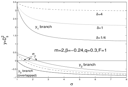
(a) $m=2,\ \beta=-0.24,\ q=0.3,\ F=1$

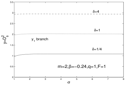
(b) $m=2,\ \beta=-0.24,\ q=1,\ F=1$

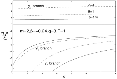
(c) $m=2,\ \beta=-0.24,\ q=3,\ F=1$

Figure 1: Aligned $D_{s}^{2}$ solution branches derived from equations (67) and (22) as functions of $\sigma\equiv 1/\eta$ by specifying $m=2$ (i.e., bar-like), $F=1$ (i.e., full discs) and $\beta=-0.24$. For each set of $\delta=1/4$ (solid curve), $1$ (dotted curve) and $4$ (dashed curve), we choose $q=0.3,\ 1$ and $3$ and show corresponding results in panels (a), (b) and (c), respectively. In panel (a), the three curves of the $y_{3}$ branch overlap with each other. Sometimes cubic equation (67) has only one real root. In panel (b), the $y_{2}$ and $y_{3}$ branches are complex for the three chosen $\delta$ values. In panel (c), the $y_{2}$ and $y_{3}$ branches are complex for the $\delta=4$ case For $\beta<1/4$, $D_{g}^{2}$ remains always greater than $D_{s}^{2}$.

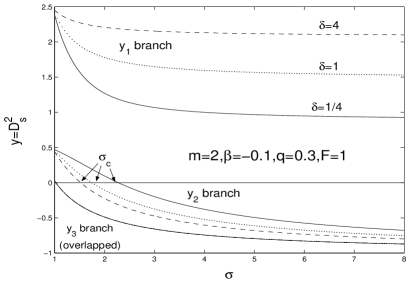
(a) $m=2,\ \beta=-0.1,\ q=0.3,\ F=1$

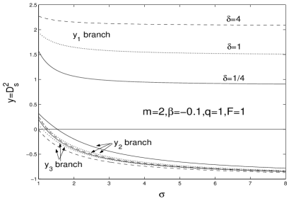
(b) $m=2,\ \beta=-0.1,\ q=1,\ F=1$

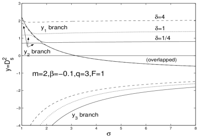
(c) $m=2,\ \beta=-0.1,\ q=3,\ F=1$

Figure 2: The solution curves of $D_{s}^{2}$ versus $\sigma$ for aligned $m=2$ (bar-like) full discs with $F=1$, $\beta=-0.1$, $\delta=1/4$ (solid curve), $1$ (dotted curve) and $4$ (dashed curve) and $q=0.3$, $1$ and $2.5$ in panels (a), (b) and (c), respectively. In panel (a), curves for the three different $\delta$ values of the $y_{3}$ branch almost overlap with each other. The same thing happens in panel (c) for large $\sigma\;\lower 4.0pt\hbox{${\buildrel\displaystyle>\over{\sim}}$}\;1.9$ in the $y_{2}$ branch and for small $\sigma$ in the $y_{1}$ branch; the dashed curve of $y_{2}$ branch almost coincides with the solid curve of $y_{1}$ branch for small $\sigma\;\lower 4.0pt\hbox{${\buildrel\displaystyle<\over{\sim}}$}\;1.9$. In panel (b) with $q=1$, the $y_{2}$ and $y_{3}$ branches are close to each other. The three curves of the $y_{3}$ branch are lower than the three curves of the $y_{2}$ branch.

As expected, the magnetic field has a very slight influence on the composite disc system when it becomes weak enough (e.g., $q=0.3$). For example, we compare our panel (b) of Fig. 3 with panel (b) of Fig. $3$ in Shen & Lou (2004b) and see that the $y_{1}$ and $y_{2}$ branches are strikingly similar to their mutual counterparts. A point in common is that when $\sigma$ becomes large (i.e., small $\eta$ corresponding to a situation where the velocity dispersion in the stellar disc is much higher than the sound speed in the magnetized gas disc), the curves tend to be more or less flat. As $q$ becomes larger, or equivalently, the Alfvén speed is comparable to or even higher than the gas sound speed, the magnetic field effect can be more prominent, especially for small $\sigma$. As $\beta$ becomes very small (e.g., $\beta=-0.24$), the magnetic field provides an attraction force, a stronger magnetic field should thus enhance the angular velocity of the magnetized gas disc (i.e., a larger $D_{g}^{2}$). Meanwhile, we see from Fig. 1 that it reduces the angular velocity for the stellar disc. Since here $D_{g}>D_{s}$, so the existence of a magnetic field enlarges the angular speed difference between the gaseous and stellar discs [see also equation (22)]. As $\beta$ becomes slightly larger (e.g., $\beta=-0.1$), $D_{g}$ still increases when $q$ grows with a greater attractive Lorentz force as expected (not shown in figures); for $D_{s}$ solution, the situation is more complicated. Here in the $\beta=-0.1$ cases with a small $\sigma$, the increase of magnetic field strength first lowers the $y_{1}$ and $y_{2}$ branches and then raises them upward when $q$ becomes sufficiently large. One interesting phenomenon is that for large $q$, the $y_{1}$ branch is flat for large $\sigma$ and the curve suddenly rises when $\sigma$ reduces to a certain value; meanwhile, the $y_{2}$ branch catches up and stretches that flat curve at small $\sigma$ [see Fig. 2(c), Fig. 3(c), Fig. 4(c)]. For large $\beta$ (e.g., $\beta=1/4$ and $\beta=0.4$), a larger $q$ directly results in an increase in all three $D_{s}^{2}$ solution branches.

We now examine the effect of varying the surface mass density ratio $\delta$. We observe a higher $y_{1}$ branch for a larger $\delta\equiv\Sigma_{0}^{g}/\Sigma_{0}^{s}$ and a higher $y_{2}$ branch for a smaller $\delta$ when $\beta$ and $q$ are small [see Fig. 1(a) and Fig. 2(a)]. This is consistent with the hydrodynamic results of Shen & Lou (2004b) where magnetic field is absent. In the presence of magnetic field, we notice a new feature that as $\beta$ and $q$ becomes sufficiently large, there emerges a ‘convergent point’ where for different $\delta$ values, some branches converge and then their relative positions are changed [see Fig. 3(b) and Fig. 3(c)]. For different branches, the convergent point varies. In addition, we see from equation (70) that since $\mathcal{X}$ is independent of $\delta$, the convergent point for $D_{g}^{2}$ solution is the same as that for the $D_{s}^{2}$ solution.

It is of some interest to consider the case in Fig. 4 for $\beta=0.4$. Different from other cases, here $D_{g}$ may become smaller than $D_{s}$ in the presence of magnetic field. This happens when $\sigma$ approaches 1 and $q$ becomes fairly large. Specifically in Fig. 4(c), $D_{g}^{2}$ solution becomes negative and thus unphysical even though $D_{s}^{2}$ remains positive.

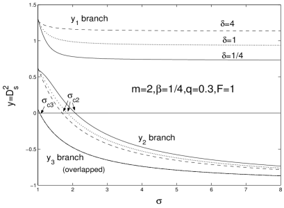
(a) $m=2,\ \beta=1/4,\ q=0.3,\ F=1$

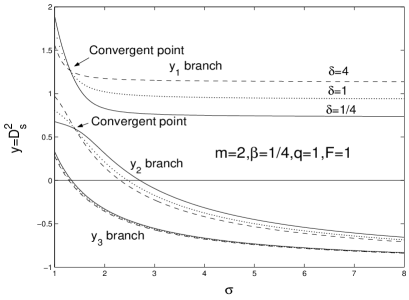
(b) $m=2,\ \beta=1/4,\ q=1,\ F=1$

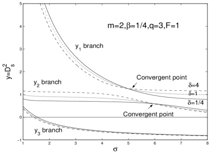
(c) $m=2,\ \beta=1/4,\ q=3,\ F=1$

Figure 3: The solution curves of $D_{s}^{2}$ versus $\sigma$ for aligned $m=2$ (bar-like) full discs with $F=1$, $\beta=1/4$, $\delta=1/4$ (solid curve), $1$ (dotted curve) and $4$ (dashed curve) and $q=0.3$, $1$ and $3$ shown in panels (a), (b), and (c), respectively. Note that for small $q$, there are three physical $D_{s}^{2}$ solutions as $\sigma$ approaches 1 and when $q$ is large enough there exists a ‘convergent point’ where branches with different $\delta$ values converge. Curves for different $\delta$ values in the $y_{3}$ branch almost merge with each other to various extents; in panel (a), the three curves of the $y_{3}$ branch overlap each other.

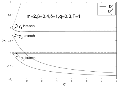
(a) $m=2,\ \beta=0.4,\ \delta=1,\ q=0.3,\ F=1$

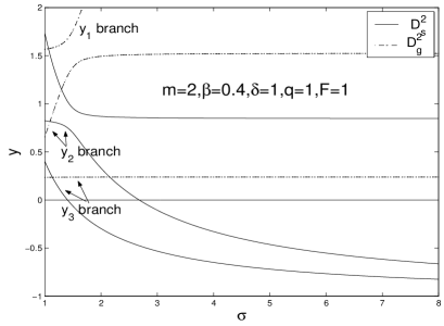
(b) $m=2,\ \beta=0.4,\ \delta=1,\ q=1,\ F=1$

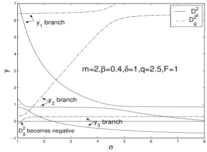
(c) $m=2,\ \beta=0.4,\ \delta=1,\ q=2.5,\ F=1$

Figure 4: The $D_{s}^{2}$ and $D_{g}^{2}$ solution curves versus $\sigma$ for aligned $m=2$ (bar-like) full discs with $\beta=0.4$, $\delta=1$, $F=1$ and $q=0.3$, $1$ and $2.5$ shown in panels (a), (b) and (c), respectively. $D_{s}^{2}$ solutions are shown in solid curves, while $D_{g}^{2}$ solutions are shown in dashed curves. The corresponding $y_{1}$, $y_{2}$, and $y_{3}$ branches are ordered from up to down, respectively. In panel (c), the lowest $D_{g}^{2}$ branch becomes negative while the corresponding $D_{s}^{2}$ branch remains positive as $\sigma$ becomes sufficiently small.

Regarding the dependence on $m$, there are not many notable features except for $m=1$. In this case, it is possible that the solution branches intersect and also there can be no physical $D_{s}^{2}$ solutions. We show a case in Fig. 5 with $\beta=-0.24$. We note that in panel (b) of Fig. 5, unlike previous $m=2$ cases, here the $y_{2}$ branch is the newly emerged branch due to the magnetic field. It intersects with $y_{3}$ branch at first [i.e., $q=0$ in Fig. 5(a)]. With the increase of magnetic field strength, it moves up and separates from the $y_{3}$ branch and then meets the $y_{1}$ branch. The result is that complex conjugate roots appear and the only real root lies along the $y_{3}$ branch which is negative and thus unphysical. Therefore, the parameter regime between the two meeting points of $y_{1}$ and $y_{2}$ branches (approximately $2.3<\sigma<3.2$) allows no stationary global MHD perturbation modes.

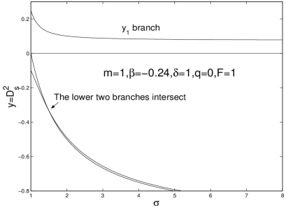
(a) $m=1,\ \beta=-0.24,\ \delta=1,\ q=0,\ F=1$

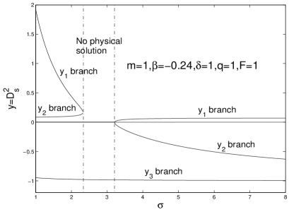
(b) $m=1,\ \beta=-0.24,\ \delta=1,\ q=1,\ F=1$

Figure 5: The $D_{s}^{2}$ solution curves versus $\sigma$ for aligned $m=1$ full discs with $\beta=-0.24$, $\delta=1$, $F=1$, and $q=0$ and 1 shown in panels (a) and (b), respectively. For $q=0$, the lower two $D_{s}^{2}$ solution branches actually intersect with each other. For $q=1$ and $2.3<\sigma<3.2$, there is no physical $D_{s}^{2}$ solutions.

3.3.3 Phase Relationships among Perturbation Variables

Phase relationships among aligned perturbation variables reflect their connections on large scales and provide models in interpreting the results from optical and synchrotron radio observations of barred or barred-spiral galaxies. In the aligned cases, most variable quantities are real (except for the $r$-component magnetic perturbation $R$) and thus they are qualitatively either ‘in phase’ or ‘out of phase’. Our main interest is to examine the phase relationships between surface mass density for the two discs and their relation to the magnetic field. To derive a quantitative expression, we start from equations $(\ref{eq:58})-(\ref{eq:60})$ and obtain

$$\begin{split}&{S^{g}}/{S^{s}}=-1-{\mathcal{M}_{A}}/{(2\pi G\Sigma_{0}^{s}r\mathcal{P}_{m})}\ ,\\ &\frac{\mathrm{i}R}{S^{g}}=\frac{mB_{0}}{\Sigma_{0}^{g}}\bigg{[}\Theta_{A}\bigg{(}1+\frac{S^{s}}{S^{g}}\bigg{)}+\Xi_{A}\bigg{]}\ ,\\ &Z={(4\beta-1)}\mathrm{i}R/{(2m)}\ .\end{split}$$ (73)

There is another version of expression for $\mathrm{i}R/S^{g}$ obtained by a combination of equations (56) and (57), namely

$$\frac{\mathrm{i}R}{S^{g}}=\frac{mB_{0}}{\Sigma_{0}^{g}}\bigg{[}\frac{4\pi G\beta\Sigma_{0}^{g}r\mathcal{P}_{m}}{\mathcal{K}_{A}}\bigg{(}1+\frac{S^{s}}{S^{g}}\bigg{)}-\frac{\mathcal{L}_{A}}{\mathcal{K}_{A}}\bigg{]}\ .$$ (74)

Equations (73) and (74) for $\mathrm{i}R/S^{g}$ are exactly the same for one can check that their combination yields the dispersion relation (65). From equation (74), it would be easier to check this consistency. Setting $\beta=0$ for the isothermal case, equation (74) reduces to equation (68) of Lou & Zou (2004) (they considered the ratio $S^{g}/Z$) as expected. Next is to evaluate these equations to express them in physical parameters. Note that $\mathrm{i}R/S^{g}$ is no longer dimensionless, to evaluate this relationship, we take the proportional factor contained in the brackets (i.e., removing $B_{0}/\Sigma_{0}^{g}$) of equation (73) for calculations. We show these results below.

$$\begin{split}&\frac{S^{g}}{S^{s}}=-1-\frac{(\mathcal{B}_{m}D_{s}^{2}-\mathcal{A}^{A}_{m})}{(D_{s}^{2}+1)}\frac{\mathcal{C}(1+\delta)}{\mathcal{P}_{m}\mathcal{A}^{A}_{m}}\ ,\\ &\frac{\mathrm{i}R}{S^{g}}\propto\frac{m}{(1+2\beta)^{2}D_{g}^{2}-(1/2-2\beta)q^{2}}\bigg{[}(1+2\beta)D_{g}^{2}-1\\ &\ \ +\frac{[D_{g}^{2}+1+{(4\beta-1)q^{2}}/{(4\beta+2)}]\mathcal{P}_{m}\delta}{\mathcal{C}(1+\delta)}\bigg{(}1+\frac{S^{s}}{S^{g}}\bigg{)}\bigg{]}\ .\end{split}$$ (75)

The first expression in equation (75) is the same as equation (42) of Shen & Lou (2004b) where a composite disc system of gravitationally coupled unmagnetized discs is analyzed.

In equations (73) and (74), there is an imaginary unit $\mathrm{i}$ on $R$ indicating that the radial component of the magnetic field perturbation lags a phase $\pi/2$ to the mass density perturbation. In the third expression of equation (73), the factor $4\beta-1$ means that the azimuthal component of the magnetic field perturbation is ahead of or lags behind the radial component of the magnetic field perturbation by $\pi/2$ for $\beta>1/4$ or $\beta<1/4$, respectively. In the special case of $\beta=1/4$, we have $Z=0$ and there is no azimuthal component of magnetic field perturbation.

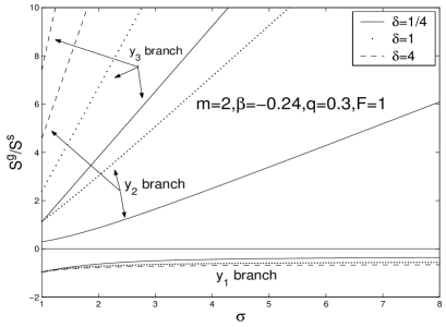
(a) $m=2,\ \beta=-0.24,\ q=0.3,\ F=1$

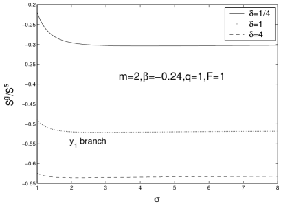
(b) $m=2,\ \beta=-0.24,\ q=1,\ F=1$

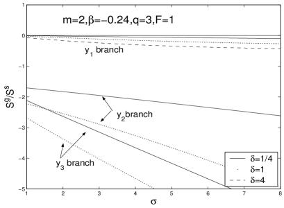
(c) $m=2,\ \beta=-0.24,\ q=3,\ F=1$

Figure 6: Phase relation curves as represented by the ratio $S^{g}/S^{s}$ for surface mass density perturbations versus $\sigma$ in the $m=2$ cases (bar-like) for full discs with $F=1$. Taking $\beta=-0.24$, we show curves with $\delta=-1/4,\ 1,\ 4$ and $q=0.3,\ 1,\ 3$ in panels (a), (b), (c), respectively. These parameters are the same as those in Fig. 1 for the convenience of reference. In panel (a), the upper, middle, and lower curves with corresponding linetypes are the $y_{3}$, $y_{2}$, and $y_{1}$ branches, respectively. In panel (b), only the $y_{1}$ branch is valid and physical. In panel (c), the curves from up to down with distinct linetypes correspond to the $y_{1}$, $y_{2}$, and $y_{3}$ branches, respectively. For $\delta=4$, there is only one real branch.

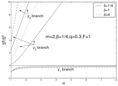
(a) $m=2,\ \beta=1/4,\ q=0.3,\ F=1$

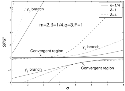
(b) $m=2,\ \beta=1/4,\ q=3,\ F=1$

Figure 7: Curves of $S^{g}/S^{s}$ ratio versus $\sigma$ for $m=2$ full discs (bar-like) with $F=1$, $\beta=1/4$, $\delta=1/4,\ 1,\ 4$ and $q=0.3,\ 3$ shown in panels (a) and (b), respectively. We adopt the same parameters as used in Fig. 3 for reference and comparison. In panel (a), the curves with different linetypes from up to down correspond to $y_{3}$, $y_{2}$, $y_{1}$ branches, respectively, and for convenience, we just label the corresponding solid curves. In panel (b), there appear ‘convergent regions’ for a larger $q$.

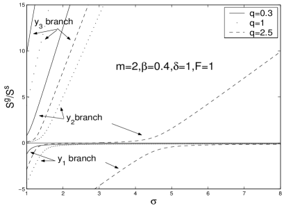
Figure 8: Curves of $S^{g}/S^{s}$ ratio versus $\sigma$ for $m=2$ full discs with $F=1$, $\beta=0.4$, $\delta=1$ and $q=0.3,\ 1,\ 2.5$, respectively. The curves from up to down correspond to $y_{3}$, $y_{2}$, and $y_{1}$ branches, respectively, and for convenience, we just label the solid curve (i.e., $q=0.3$).

The phase relationships for surface mass densities of aligned perturbations are displayed in Fig. 6$-$Fig. 8. In these three figures, we adopt the same parameters as used in computing the dispersion relations shown in Fig. 1$-$Fig. 4 for complete information. For the convenience of statement, we still refer to the phase relation curves as $y_{1}$, $y_{2}$, and $y_{3}$ branches corresponding to the $y_{1}$, $y_{2}$ and $y_{3}$ of $D_{s}^{2}$ solutions in the dispersion relation.

The magnetic field influences the perturbation mass density ratio. We demonstrate a few examples in Fig. 7 and Fig. 8. In the case of a small $q$ (e.g., $q=0.3$), the $y_{1}$ branch is negative (i.e., out of phase) while $y_{2}$ and $y_{3}$ branches are positive (i.e., in phase). However, as the magnetic field increases, the $y_{2}$ branch becomes negative for small $\sigma$. This means that for aligned stationary MHD density waves, the density phase relationship between the two scale-free discs are out of phase for super fast MHD density waves and in phase for fast MHD density waves. For the middle one, the mass density ratios are in phase in the regime of a weaker magnetic field but are out of phase in the regime of a stronger magnetic field.

We explore phase relationships of surface mass density perturbations with several different $\delta$ values in Fig. 6 and Fig.  7. One might expect that large $\delta$ leads to higher $S^{g}/S^{s}$ ratio; however, this is not always the case, especially when both $\beta$ and $q$ are large (e.g., Fig. 7 and Fig. 8). We notice ‘convergent regions’ where the phase relation curves with different $\delta$ ratios seem to converge. By carefully examining these phase curves, they do not actually converge but just become very close to each other. This phenomenon results from a complex interaction between the magnetic field and the two-fluid disc system and is a new feature in our model as compared with previous works [e.g., Lou & Shen (2003); Lou & Zou (2004); Shen & Lou (2004b); Lou & Zou 2006].

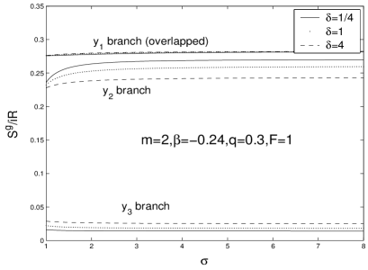
(a) $m=2,\ \beta=-0.24,\ q=0.3,\ F=1$

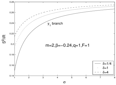
(b) $m=2,\ \beta=-0.24,\ q=1,\ F=1$

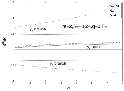
(c) $m=2,\ \beta=-0.24,\ q=3,\ F=1$

Figure 9: Perturbation phase relation curves for gas surface mass density and radial component magnetic field in the $m=2$ (bar-like) cases for full discs. Taking $\beta=-0.24$, we show curves with $\delta=1/4,\ 1,\ 4$ and $q=0.3,\ 1,\ 3$ in panels (a), (b), and (c), respectively. From relation (73), we see that $S^{g}/(\mathrm{i}R)$ and $S^{g}/Z$ are proportional to each other with a sign change depending on whether $\beta<1/4$ or not.

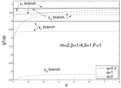
Figure 10: Curves of $S^{g}/(\mathrm{i}R)$ ratio versus $\sigma$ for $m=2$ full discs with $F=1$, $\beta=1/4$, $\delta=1$ and $q=0.3,\ 1,\ 2$. The upper, middle and lower branches with different linetypes correspond to $y_{1}$, $y_{2}$ and $y_{3}$ branches, respectively. For the solid curves with $q=0.3$, the upper two branches $y_{1}$ and $y_{2}$ are quite close to each other and the negative $y_{3}$ branch approaches zero.

We now examine phase relationships between gas mass density perturbation and the radial component of magnetic field perturbation (Fig. 9 and Fig. 10) with $m=2$ (bar-like). From equation (74), we know that $S^{g}/Z$ is proportional to $S^{g}/(\mathrm{i}R)$ with a factor $2m/(4\beta-1)$. When $\beta\neq 1/4$ the phase curves regarding $S^{g}/Z$ and $S^{g}/(\mathrm{i}R)$ are the same in shape. For $\beta>1/4$, $S^{g}/Z$ and $S^{g}/(\mathrm{i}R)$ are of the same sign, while for $\beta<1/4$, $S^{g}/Z$ and $S^{g}/(\mathrm{i}R)$ are of the opposite sign. For $\beta=1/4$, we simply have $Z=0$. For these reasons we just discuss $S^{g}/(\mathrm{i}R)$ for convenience; the information of $S^{g}/Z$ can be readily derived accordingly. In the case of $\beta=-0.24$, we already know that the $y_{1}$ branch is always physical. Here in Fig. 9, we see that $\mathrm{i}R$ and $S^{g}$ remain always in phase, and therefore from equation (73), we know that $Z$ and $S^{g}$ are out of phase. The enhancement of the magnetic field lowers the ratio $S^{g}/(\mathrm{i}R)$, as a stronger magnetic field tends to induce a larger magnetic perturbation. In the case of larger $\beta$, the dependence of this ratio to the magnetic field is somehow more sensitive. We take the case of $\beta=1/4$ as an example of illustration. In this case, the azimuthal magnetic perturbation vanishes, with a nonzero $r-$component magnetic field perturbation. We see in Fig. 10 that when $q$ is small, the $y_{1}$ and $y_{2}$ branches are positive and are very close to each other. The $y_{3}$ branch is negative and borders on zero (recall that $y_{2}$ and $y_{3}$ branches can be physical when $\sigma<\sigma_{c2}$ or $\sigma<\sigma_{c3}$). As $q$ increases, all three branches lower and the $y_{2}$ branch intersects zero indicating a phase relation reversal across the critical point. When $q$ is increased further, the entire $y_{2}$ branch becomes negative.

3.3.4 Partial Discs Embedded in a Dark Matter Halo

Coplanar aligned MHD perturbation structures in full scale-free discs are extensively discussed above. For partial discs with factor $F<1$, we expect that the introduction of an axisymmetric dark matter halo may lead to some novel features. In fact, through numerical computations we see that new features manifest mainly through the $m=1$ case as shown in Fig. 11.

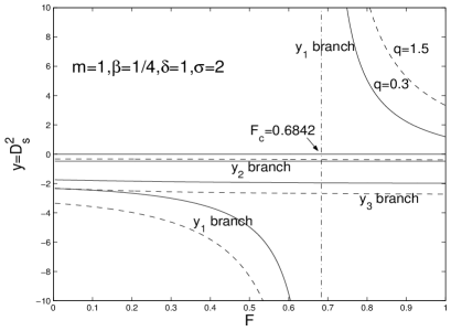
(a) $m=1,\ \beta=1/4,\ \delta=1,\ \sigma=2$

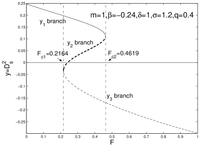
(b) $m=1,\ \beta=-0.24,\ \delta=1,\ \sigma=1.2,\ q=0.4$

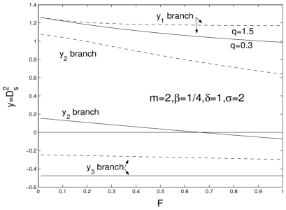
(c) $m=2,\ \beta=1/4,\ \delta=1,\ \sigma=2$

Figure 11: Dispersion relationships of $D_{s}^{2}$ versus $F$ variation for a composite system of partial scale-free discs. There are a few interesting features in the case $m=1$. There is only one real $D_{s}^{2}$ root in panel (b), while the other two roots are complex conjugates. It happens that the three $D_{s}^{2}$ branches are connected smoothly. In panel (c) for $m=2$, $y_{1}$ branch represents the upper two curves ($q=1.5$ for dashed curve and $q=0.3$ for solid curve). The $y_{2}$ branch is labeled separately and the $y_{3}$ branch represents the lower two curves.

We first note that one of the $D_{s}^{2}$ or $D_{g}^{2}$ solutions diverges for the cubic coefficient $C^{A}_{3}=0$. As our $C^{A}_{3}$ is proportional to $C_{2}$ of equation (48) in Shen et al. (2005), we expect to have a similar result in this aspect. This phenomenon appears at $m=1$. Let $\beta=1/4$ and we see in Fig. 11(a) the divergent point lies at $F_{c}\simeq 0.6842$ which is exactly the same as that in the analysis of Shen et al. (2005), and we have an additional $y_{3}$ branch (although negative and thus unphysical). Another difference is that here the $y_{2}$ branch is also negative and therefore the only physical solution lies in the positive portion of $y_{1}$ solutions. The direct consequence is that for $0<F\leq F_{c}$, there can be no physical solutions.

We also evaluate the $m=1$ cases with different $\beta$ values. For a sufficiently small $\beta$ (e.g., $\beta=-0.24$), there appears a kind of discontinuity seen in Fig. 11(b). Actually, the range of $F$ is divided into three regimes. For $0<F<F_{c1}$, only $y_{1}$ branch exists and the other two $D_{s}^{2}$ roots are complex conjugates. For $F_{c1}\leq F\leq F_{c2}$, all three branches are real. For $F_{c2}<F\leq 1$, only the $y_{3}$ branch exists. Since $y_{3}$ branch is negative, there is no physical solution for $F_{c2}<F\leq 1$. Immediately at $F=F_{c2}$, there emerges suddenly a new solution (double roots), and this solution then bifurcates into two branches as $F$ becomes smaller. The $y_{2}$ branch turns negative before $F$ encounters $F_{c1}$ and from then on there is only one physical solution for smaller $F$.

For $m=2$ bar-like configurations, we take $\beta=1/4$, $\delta=1$, $\sigma=2$ with $q=0.3$ and $1.5$ respectively to obtain solutions in panel (c) of Fig. 11. For this set of parameters, the $y_{1}$ branch remains always positive while the $y_{3}$ branch remains always negative. Whether the $y_{2}$ branch is positive or not depends on the choice of parameters $F$ and $q$. It is clear that an increase of magnetic field raises all three branches. This raises the $y_{1}$ branch only slightly but greatly lifts the lower two branches. Especially for $y_{2}$ branch, only smaller $F$ values can ensure a positive $y_{2}$ when $q$ is sufficiently small, while a sufficiently large $q$ parameter actually makes $y_{2}$ positive for all $0<F\leq 1$. For other values of $m$, the global aligned MHD perturbation patterns and trends of variation are qualitatively similar.

4 Unaligned MHD Configurations
  of Global Logarithmic Spirals

In this section, we study the unaligned MHD perturbations by introducing a special yet useful potential-density pair referred to as the logarithmic spirals. We first derive the MHD dispersion relation for the composite system of two coupled scale-free discs. We then focus on computations of $m\geq 1$ cases. Finally, we study the $m=0$ case which leads to the discussion of the axisymmetric marginal stability.

4.1 Stationary MHD Dispersion Relation
   for Global Logarithmic Spirals

To construct global logarithmic spiral MHD perturbations, we take the potential-density pair in the form of

$$\begin{split}&S^{i}(r)=\epsilon^{i}r^{-3/2}\mathrm{exp}(\mathrm{i}\xi\mathrm{ln}r)\ ,\\ &V^{i}(r)=-2\pi GrS^{i}\mathcal{N}_{m}(\xi)\ ,\end{split}$$ (76)

where $\epsilon^{i}$ is a small constant amplitude coefficient, superscript $i$ denotes either $g$ or $s$ for either gas or stellar discs, $\xi$ represents the radial wavenumber and the Kalnajs function $\mathcal{N}_{m}(\xi)$ is defined by

$$\mathcal{N}_{m}(\xi)=\frac{\Gamma(m/2+\mathrm{i}\xi/2+1/4)\Gamma(m/2-\mathrm{i}\xi/2+1/4)}{2\Gamma(m/2+\mathrm{i}\xi/2+3/4)\Gamma(m/2-\mathrm{i}\xi/2+3/4)}\$$ (77)

(Kalnajs, 1971). In potential-density pair (76), the perturbed surface mass density is complex, with an amplitude radial scaling of $r^{-3/2}$ and a phase factor $r^{\mathrm{i}\xi}$ for radial oscillations. The relevant radial variations are no longer the same as those of the background equilibrium unless $\beta=1/4$. In fact, there can be more general potential-density pairs as noted in Shen & Lou (2004b). For the analysis of the marginal stability problem, expression (76) is used such that the dispersion relation (98) derived later is real on both sides, and this choice of scale factor satisfies the scale-free condition in the perturbation equations. The phase factor is the key to establish global logarithmic spiral patterns. We call it logarithmic spirals because the dependence of the phase factor on $r$ follows the logarithmic function. Kalnajs function (77) is an even function in $\xi$ and thus a consideration of $\xi\geq 0$ (i.e., leading MHD density waves) suffices.

We now derive the MHD dispersion relation for global logarithmic spirals with $m\geq 1$ cases using equations $(\ref{eq:41})-(\ref{eq:43})$, (48) together with (76). With radial scalings of $S\propto r^{-3/2+\mathrm{i}\xi}$, $V\propto r^{-1/2+\mathrm{i}\xi}$, $U\propto r^{-1/2+\beta+\mathrm{i}\xi}$ and $J\propto r^{1/2+\beta+\mathrm{i}\xi}$, all quantities in equations $(\ref{eq:41})-(\ref{eq:43})$ and (48) are scale-free; these equations become

$$m\Omega_{g}S^{g}-(1/2-\mathrm{i}\xi+\beta)\frac{\Sigma_{0}^{g}}{r}\mathrm{i}U^{g}+\frac{m\Sigma_{0}^{g}}{r^{2}}J^{g}=0\ ,$$ (78)

$$\begin{split}&\bigg{\{}m\Omega_{g}-\frac{C_{A}^{2}[2m^{2}-\mathrm{i}\xi(1-4\beta)+2\xi^{2}]}{2m\Omega_{g}r^{2}}\bigg{\}}\mathrm{i}U^{g}=\\ &\bigg{[}(1-2\mathrm{i}\xi)\pi G\mathcal{N}_{m}-\frac{(1-2\mathrm{i}\xi)a_{g}^{2}+(1-4\beta)C_{A}^{2}}{2r\Sigma_{0}^{g}}\bigg{]}S^{g}\\ &\quad\qquad\qquad\qquad+(1-2\mathrm{i}\xi)\pi G\mathcal{N}_{m}S^{s}-\frac{2\Omega_{g}}{r}J^{g}\ ,\end{split}$$ (79)

$$\begin{split}m\Omega_{g}&J^{g}+\bigg{[}(1-\beta)r\Omega_{g}-\frac{C_{A}^{2}(1-4\beta)}{2r\Omega_{g}}\bigg{]}\mathrm{i}U^{g}=\\ &\quad\qquad mr\bigg{(}2\pi G\mathcal{N}_{m}-\frac{a_{g}^{2}}{r\Sigma_{0}^{g}}\bigg{)}S^{g}+2\pi Gmr\mathcal{N}_{m}S^{s}\ ,\end{split}$$ (80)

$$Z=-\mathrm{i}\xi\frac{B_{0}\mathrm{i}U^{g}}{m\Omega_{g}r}\ ,\qquad\qquad\qquad R=\frac{B_{0}U^{g}}{r\Omega_{g}}$$ (81)

for the magnetized gas disc and

$$\begin{split}&\bigg{[}\frac{(m^{2}-2+2\beta)\Omega_{s}^{2}r^{2}}{m^{2}+\xi^{2}+2\beta+1/4}-a_{s}^{2}+2\pi Gr\Sigma_{0}^{s}\mathcal{N}_{m}\bigg{]}S^{s}\\ &\qquad\qquad\qquad\qquad\qquad+2\pi Gr\Sigma_{0}^{s}\mathcal{N}_{m}S^{g}=0\end{split}$$ (82)

for the stellar disc. Equations $(\ref{eq:78})-(\ref{eq:81})$ are the same as equation (65) in Shen et al. (2005) for a single magnetized scale-free disc by setting $S^{s}=0$ and equation (82) is exactly the same as the first equation of (68) in Shen & Lou (2004b). A combination of equations $(\ref{eq:78})-(\ref{eq:80})$ and (82) gives the full solution for the stationary dispersion relation of the gravitational coupled MHD discs for logarithmic spirals. Similar to the aligned cases, these are homogeneous linear equations in terms of $(S^{g},\ S^{s},\ U^{g},\ J^{g})$. For non-trivial solutions, the determinant of the coefficients of equations $(\ref{eq:78})-(\ref{eq:80})$ and (82) should vanish. The result is the stationary MHD dispersion relation. As necessary requirements, we expect that in special cases, this dispersion relation will reduce to those discussed by Shen et al. (2005) or Shen & Lou (2004b). Meanwhile, we solve the above equations directly to reveal physical contents.

A combination of equations (78) and (80) leads to two expressions of $\mathrm{i}U^{g}$ and $J^{g}$ in terms of $S^{g}$ and $S^{s}$, namely

$$\begin{split}&\mathrm{i}U^{g}={m\Omega_{g}r}[(\Theta_{S}+\Xi_{S})S^{g}+\Theta_{S}S^{s}]/\Sigma_{0}^{g}\ ,\\ &J^{g}={\Omega_{g}r^{2}}\{[-1+(1/2-\mathrm{i}\xi+\beta)(\Theta_{S}+\Xi_{S})]S^{g}\\ &\qquad\qquad\qquad\qquad+(1/2-\mathrm{i}\xi+\beta)\Theta_{S}S^{s}\}/\Sigma_{0}^{g}\ ,\end{split}$$ (83)

where, for notational simplicity, we denote

$$\begin{split}&\Theta_{S}\equiv{2\pi Gr\mathcal{N}_{m}\Sigma_{0}^{g}}/{\Delta_{S}}\ ,\\ &\Xi_{S}\equiv{(-a_{g}^{2}+\Omega_{g}^{2}r^{2})}/{\Delta_{S}}\ ,\\ &\Delta_{S}\equiv(3/2-\mathrm{i}\xi)\Omega_{g}^{2}r^{2}+(2\beta-1/2)C_{A}^{2}\ .\end{split}$$ (84)

We use the subscript _S to indicate the logarithmic ‘spiral cases’. Note that $\Theta_{S}$ and $\Xi_{S}$ are two dimensionless constant parameters. A substitution of equation (83) into equation (79) and a further combination with equation (82) lead to

$$\begin{split}[\mathcal{K}_{S}(\Theta_{S}+\Xi_{S})+\mathcal{L}_{S}-(1-2\mathrm{i}\xi)\pi G\Sigma_{0}^{g}r\mathcal{N}_{m}]&S^{g}\\ \quad+[\mathcal{K}_{S}\Theta_{S}-(1-2\mathrm{i}\xi)\pi G\Sigma_{0}^{g}r\mathcal{P}_{m}]&S^{s}=0\ ,\\ 2\pi G\Sigma_{0}^{s}r\mathcal{N}_{m}S^{g}+(\mathcal{M}_{S}+2\pi G\Sigma_{0}^{s}r\mathcal{N}_{m})&S^{s}=0\ ,\end{split}$$ (85)

where, for notational simplicity, we further define

$$\begin{split}&\mathcal{K}_{S}\equiv(m^{2}+2\beta+1-2\mathrm{i}\xi)\Omega_{g}^{2}r^{2}\\ &\qquad\ \qquad-[m^{2}-\mathrm{i}\xi(1/2-2\beta)+\xi^{2}]C_{A}^{2}\ ,\\ &\mathcal{L}_{S}\equiv(1/2-2\beta)C_{A}^{2}-2\Omega_{g}^{2}r^{2}+(1/2-\mathrm{i}\xi)a_{g}^{2}\ ,\\ &\mathcal{M}_{S}\equiv\frac{(m^{2}+2\beta-2)\Omega_{s}^{2}r^{2}}{(m^{2}+\xi^{2}+2\beta+1/4)}-a_{s}^{2}\ .\end{split}$$ (86)

We can derive the stationary MHD dispersion relation for global logarithmic spirals by calculating the coefficient determinant of equations (82) and (85). After manipulations and rearrangements, we obtain

$$\begin{split}&({\Delta_{S}}/\mathcal{K}_{S})[\mathcal{K}_{S}(\Theta_{S}+\Xi_{S})+\mathcal{L}_{S}-(1-2\mathrm{i}\xi)\pi G\Sigma_{0}^{g}r\mathcal{N}_{m}]\\ &\quad\qquad\times(\mathcal{M}_{S}+2\pi G\Sigma_{0}^{s}r\mathcal{N}_{m})\\ &\ \ \qquad\quad=4\pi^{2}G^{2}\Sigma_{0}^{g}\Sigma_{0}^{s}r^{2}\mathcal{N}_{m}^{2}[1-(1/2-\mathrm{i}\xi){\Delta_{S}}/{\mathcal{K}_{S}}]\ .\end{split}$$ (87)

In equation (87), the left-hand side consists of two factors. One can show that the factor in the left brackets is exactly the dispersion relation in a single coplanar magnetized disc discussed by Shen et al. (2005) and the second factor in parentheses denotes the dispersion relation of a single scale-free stellar disc. The right-hand side denotes the mutual gravitational coupling between the two scale-free discs. By setting $\beta=0$ for the isothermal case, equation (87) reduces to equation (106) in Lou & Zou (2004) where isothermal fluid-magnetofluid discs are investigated.

In all calculations of this subsection, the equations for logarithmic spirals are strikingly similar to those of the aligned perturbations. If we replace $\mathcal{P}_{m}$ by $\mathcal{N}_{m}$ and partly replace $2\beta$ by $1/2-\mathrm{i}\xi$, this similarity arises in the expression of the perturbation equations. We assert that the similarity in structure must lead to the similarity in concrete expressions of the dispersion relation between the two cases. We show this fact in the next subsection.

4.2 Stationary Logarithmic Spiral Configurations

4.2.1 $D_{s}^{2}$ and $D_{g}^{2}$ Solutions of the Dispersion Relation

We now evaluate the spiral dispersion relation for $m\geq 1$ cases numerically to show the dependence of $D_{g}^{2}$ or $D_{s}^{2}$ on other dimensionless parameters (i.e., $m,\ \beta,\ \eta,\ \delta,\ q,\ F$). Similar to the aligned cases, we choose to calculate the coefficient determinant of equations $(\ref{eq:78})-(\ref{eq:80})$ and (82). We leave details of onerous calculations to Appendix C where the simplified determinant is shown explicitly. After careful calculations and simplifications, we obtain the MHD dispersion relation as cubic polynomial equation in terms of $D_{g}^{2}$. It is satisfying to see that this dispersion relation can be expressed in the exactly same form as that of the aligned cases merely by a substitution of notations. We write

$$\begin{split}\mathcal{A}^{S}_{m}(\beta,\ \xi)&\equiv m^{2}+\xi^{2}+2\beta+1/4\ ,\\ \mathcal{H}^{S}_{m}(\beta,\ \xi)&\equiv{\mathcal{A}^{S}_{m}\mathcal{N}_{m}}/{\mathcal{C}}+\mathcal{B}_{m}\ .\\ \end{split}$$ (88)

We still use the notations $\mathcal{B}_{m}(\beta)$ and $\mathcal{C}(\beta)$ as defined in equation (66). Now the stationary MHD dispersion relation can be written in terms of $y\equiv D_{g}^{2}$, namely

$$C^{S}_{3}y^{3}+C^{S}_{2}y^{2}+C^{S}_{1}y+C^{S}_{0}=0\ .$$ (89)

The four coefficients $C^{S}_{3}$, $C^{S}_{2}$, $C^{S}_{1}$, $C^{S}_{0}$ are functions of dimensionless parameters $m,\ \beta,\ \delta,\ \eta,$ and $q^{2}$ defined by

$$\begin{split}&C^{S}_{3}\equiv\mathcal{B}_{m}\mathcal{H}^{S}_{m}\eta\ ,\\ &C^{S}_{2}\equiv\bigg{[}(\mathcal{B}_{m}-\mathcal{A}^{S}_{m})\mathcal{H}^{S}_{m}+\frac{(\mathcal{A}^{S}_{m}+\mathcal{B}_{m})(\mathcal{H}^{S}_{m}-\mathcal{B}_{m})\delta}{(1+\delta)}\bigg{]}\eta\\ &\qquad\qquad-\frac{(\mathcal{A}^{S}_{m}+\mathcal{B}_{m})(\mathcal{H}^{S}_{m}\delta+\mathcal{B}_{m})}{(1+\delta)}+C^{S}_{2Q}q^{2}\ ,\\ &C^{S}_{1}\equiv\bigg{[}-\mathcal{A}^{S}_{m}\mathcal{H}^{S}_{m}+\frac{(\mathcal{A}^{S}_{m}+\mathcal{B}_{m})(\mathcal{H}^{S}_{m}-\mathcal{B}_{m})\delta}{(1+\delta)}\bigg{]}\eta\\ &+(\mathcal{A}^{S}_{m}+\mathcal{B}_{m})^{2}-\frac{(\mathcal{A}^{S}_{m}+\mathcal{B}_{m})(\mathcal{H}^{S}_{m}\delta+\mathcal{B}_{m})}{(1+\delta)}+C^{S}_{1Q}q^{2}\ ,\\ &C^{S}_{0}\equiv C^{S}_{0Q3}q^{6}+C^{S}_{0Q2}q^{4}+C^{S}_{0Q1}q^{2}\ ,\end{split}$$ (90)

where the following five coefficients are further defined by

$$\begin{split}&C^{S}_{2Q}\equiv\frac{m^{2}(4\beta-1)-2\mathcal{A}^{S}_{m}+8\beta^{2}-20\beta+6}{2(1+\delta)}(\mathcal{H}^{S}_{m}+\mathcal{B}_{m}\delta)\eta\\ &\qquad\qquad-\frac{4(1-2\beta)\mathcal{A}^{S}_{m}-(1+2\beta)}{(4\beta+2)(1+\delta)}\frac{\mathcal{B}_{m}\mathcal{N}_{m}}{\mathcal{C}}\delta\eta\ ,\\ \end{split}$$

$$\begin{split}&C^{S}_{1Q}\equiv-\frac{\mathcal{A}^{S}_{m}+5\beta-2}{(1+\delta)}(\mathcal{H}^{S}_{m}+\mathcal{B}_{m}\delta)\eta\\ &\qquad\quad-\frac{\mathcal{A}^{S}_{m}(4\beta-3)+2\beta+1}{(4\beta+2)(1+\delta)}\bigg{(}\mathcal{H}^{S}_{m}+\mathcal{B}_{m}\delta-\frac{2\mathcal{B}_{m}\mathcal{N}_{m}\delta}{\mathcal{C}}\bigg{)}\eta\\ &\qquad\quad-\frac{\mathcal{A}^{S}_{m}(4\beta-3)+2\beta+1}{(4\beta+2)(1+\delta)}\frac{\mathcal{N}_{m}}{\mathcal{C}}(\mathcal{A}^{S}_{m}+\mathcal{B}_{m})\delta\\ &\qquad\quad+(\mathcal{A}^{S}_{m}+\mathcal{B}_{m})(\mathcal{A}^{S}_{m}+5\beta-2)\ ,\\ \end{split}$$

$$\begin{split}&C^{S}_{0Q3}\equiv-\frac{(4\beta-1)^{3}(\mathcal{H}^{S}_{m}+\mathcal{B}_{m}\delta)\eta}{2(4\beta+2)^{2}(1+\delta)}\\ &\qquad\ \ \ -\frac{(4\beta-1)^{2}(2\mathcal{A}^{S}_{m}-2\beta-1)}{(4\beta+2)^{3}(1+\delta)}\frac{\mathcal{B}_{m}\mathcal{N}_{m}}{\mathcal{C}}\delta\eta\ ,\\ \end{split}$$

$$\begin{split}&C^{S}_{0Q2}\equiv\frac{(4\beta-1)}{(4\beta+2)}\bigg{[}\frac{(4\beta-1)}{2}+\frac{2\mathcal{A}^{S}_{m}-2\beta-1}{(4\beta+2)(1+\delta)}\frac{\mathcal{N}_{m}}{\mathcal{C}}\delta\bigg{]}\\ &\qquad\quad\times(\mathcal{A}^{S}_{m}+\mathcal{B}_{m})-\frac{(4\beta-1)^{2}(\mathcal{H}^{S}_{m}+\mathcal{B}_{m}\delta)\eta}{2(4\beta+2)(1+\delta)}\\ &\quad+\frac{(4\beta-1)(2\mathcal{A}^{S}_{m}-2\beta-1)}{(4\beta+2)^{2}(1+\delta)}\bigg{(}\mathcal{H}^{S}_{m}+\mathcal{B}_{m}\delta-\frac{2\mathcal{B}_{m}\mathcal{N}_{m}\delta}{\mathcal{C}}\bigg{)}\eta\ ,\\ \end{split}$$

$$\begin{split}&C^{S}_{0Q1}\equiv\frac{(2\mathcal{A}^{S}_{m}-2\beta-1)}{(4\beta+2)(1+\delta)}\bigg{(}\mathcal{H}^{S}_{m}+\mathcal{B}_{m}\delta-\frac{\mathcal{B}_{m}\mathcal{N}_{m}\delta}{\mathcal{C}}\bigg{)}\eta\\ &\qquad-\frac{(2\mathcal{A}^{S}_{m}-2\beta-1)}{(4\beta+2)(1+\delta)}\bigg{(}1+\delta-\frac{\mathcal{N}_{m}}{\mathcal{C}}\delta\bigg{)}(\mathcal{A}^{S}_{m}+\mathcal{B}_{m})\ .\end{split}$$ (91)

Before solving dispersion relation (89), we see qualitatively the dependence of $y\equiv D_{g}^{2}$ on other dimensionless parameters. Similar to the aligned cases, we have $C^{S}_{0}=0$ for $q=0$ and meanwhile, $C^{S}_{3},\ C^{S}_{2},\ C^{S}_{1}$ are exactly the same as $C_{2},\ C_{1},\ C_{0}$ respectively in equation (72) of Shen & Lou (2004b). By setting $\eta=0$ and $\delta\rightarrow\infty$, we have $C_{3}=0$ and the coefficients actually reduce to the situation of a single MHD scale-free disc analyzed by Shen et al. (2005) [see their equations (70)]. We also point out that by setting $\beta=1/4$ and $\xi=0$, we have $\mathcal{N}_{m}(1/4,\ 0)=\mathcal{P}_{m}(1/4)$ and $\mathcal{A}_{m}(1/4,\ 0)=\mathcal{A}^{S}_{m}(0)$, this logarithmic spiral case goes back to the aligned $\beta=1/4$ case as expected.

Equation (89) is cubic in $y\equiv D_{g}^{2}$. We can also readily cast equation (89) in terms of $D_{s}^{2}$ instead of $D_{g}^{2}$. This is exactly parallel to what we have done in the analysis of the aligned cases and we would not repeat the steps here. For notational clarity, we should add ^′ to the coefficients of the cubic equation for $D_{s}^{2}$ such as $C^{S^{\prime}}_{0}$ and so forth, similar to the aligned cases. However, since $D_{s}^{2}$ will be frequently used, we denote $y=D_{s}^{2}$ instead of $y^{\prime}$ from now on unless otherwise stated.

4.2.2 Dependence of $D_{s}^{2}$ Solutions with
   Other Dimensionless Parameters

As we have shown before, the dispersion relation for global logarithmic spirals is expressed in the same form as that for aligned perturbations, indicating that the behaviours of the two cases bear certain similarities. Compared with the aligned cases, the differences should arise only from the substitutions of $\mathcal{A}^{A}_{m}(\beta)$ by $\mathcal{A}^{S}_{m}(\beta,\ \xi)$ and $\mathcal{P}_{m}(\beta)$ by $\mathcal{N}_{m}(\xi)$, respectively. For logarithmic spiral perturbations, there is one more parameter $\xi$ corresponding to the radial wavenumber. This parameter is important for forming large-scale structures in spiral galaxies. On the one hand, we are interested in the influence of $\xi$ on behaviours of $D_{s}^{2}$ solution. On the other hand, by analogy we can imagine that the dependence of $D_{s}^{2}$ solution on parameter $\eta$ should be similar to that of the aligned cases. For these two reasons, we present our figures in $\xi-y$ plane where $y=D_{s}^{2}$. We focus on the $m=2$ case (viz., two-armed spirals). For cases of different $\beta$ values, we will show in Fig. 12$-$Fig. 14. The $m=1$ case is shown in Fig. 15 briefly. We also show results for partial discs in Fig. 16.

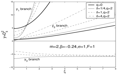
(a) $m=2,\ \beta=-0.24,\ \sigma=1,\ F=1$

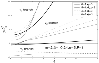
(b) $m=2,\ \beta=-0.24,\ \sigma=5,\ F=1$

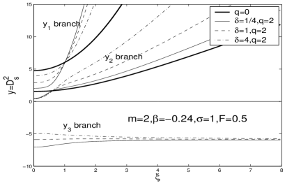
(c) $m=2,\ \beta=-0.24,\ \sigma=1,\ F=0.5$

Figure 12: $D_{s}^{2}$ solution branches of equations (89) and (22) as functions of radial wave number $\xi$ with specified parameters $m=2$ and $\beta=-0.24$. When $q=0$, our cases naturally reduce to the unmagnetized coupled discs analyzed by Shen & Lou (2004b) where there are two roots corresponding to faster and slower density waves (Lou & Fan 1998b). For the convenience of comparison, we draw this case of $q=0$ in boldface solid curves. When $\sigma=1$ and $q=0$, the solution is independent of $\delta$ (Shen & Lou, 2004b). Setting $q=2$, we then show the solutions with $\delta=1/4,\ 1$ and 4 which are displayed in solid, dashed and dash-dotted curves, respectively. We examine full discs with $\sigma=1$ and $\sigma=5$ shown in panels (a) and (b), while for a partial disc, we show a case with $\sigma=1$ and $F=0.5$.

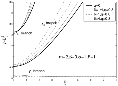
(a) $m=2,\ \beta=0,\ \sigma=1,\ F=1$

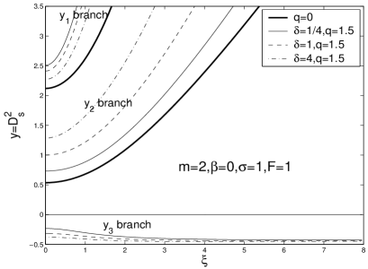
(b) $m=2,\ \beta=0,\ \sigma=1,\ F=1$

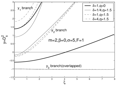
(c) $m=2,\ \beta=0,\ \sigma=5,\ F=1$

Figure 13: $D_{s}^{2}$ solution curves versus $\xi$ for a logarithmic spiral case with $m=2,\ \beta=0,\ F=1$. Magnetic field has a considerable influence on the disc system [see panels (a) and (b)]. A weak magnetic field results in a physical $y_{3}$ solution but when the magnetic field strength becomes stronger, this $y_{3}$ solution falls negative. In panel (c), we show the influence of $\sigma$, where the three curves of $y_{3}$ branch pact together.

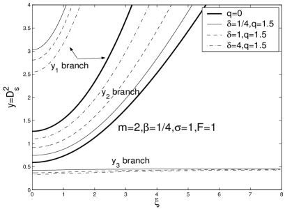
(a) $m=2,\ \beta=1/4,\ \sigma=1,\ F=1$

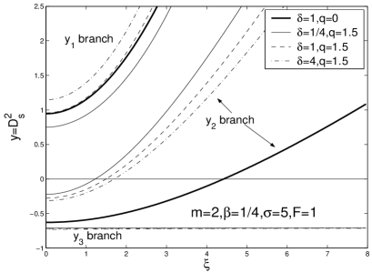
(b) $m=2,\ \beta=1/4,\ \sigma=5,\ F=1$

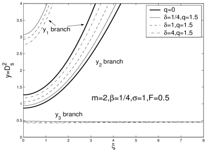
(c) $m=2,\ \beta=1/4,\ \sigma=1,\ F=0.5$

Figure 14: $D_{s}^{2}$ solution curves versus $\xi$ for a logarithmic spiral with $m=2$ (two-armed spirals) and $\beta=1/4$. By setting $q=1.5$, we show the solutions with $\delta=1/4,\ 1$ and 4, respectively. The cases for full discs with $\sigma=1$ and $\sigma=5$ are shown in panels (a) and (b), respectively. For a partial disc, we set $\sigma=1$ and $F=0.5$ and show the results in panel (c). The three curves of branch $y_{3}$ overlap with each other.

Similar to the aligned cases, the $y_{1}$ and $y_{2}$ branches correspond to the unmagnetized solutions of Lou & Fan (1998b) and Shen & Lou (2004b) and $y_{3}$ is an extra solution (i.e., SMDWs) due to the very existence of magnetic field. Meanwhile, the upper two branches are monotonically increasing with the increase of $\xi$, while the $y_{3}$ branch remains always flat as $\xi$ varies. The $y_{3}$ branch is sensitive to the $q$ variation. This is a sign that the $y_{3}$ solution is the direct result of the magnetic field. Generally, the $y_{1}$ branch remains always positive, the $y_{2}$ branch can be either positive or negative and the lowest $y_{3}$ branch is mostly negative and thus unphysical. There are critical values of $\xi$ at which these branches change signs. These critical values are determined by $C^{S^{\prime}}_{0}=0$. As they cannot be evaluated analytically, we simply show their presence in the figures. In each figure, we choose $\sigma=1$ and $\sigma=5$ and see that all three branches are lowered for larger values of $\sigma$ as expected. This trend of variation is similar to that in the aligned cases.

For logarithmic spiral cases with $m=2$, the ‘convergent point’ is a common phenomenon where curves with different $\delta$ values tend to converge at a certain point. For a small $\beta$ (e.g., $\beta=-0.24$), there is no convergent point in the aligned cases but here the variation of $\xi$ produces this convergent point. For larger $\beta$ values (e.g., $\beta=0,\ 1/4$), the situation becomes similar to the aligned cases where variations of $\sigma$ lead to the existence of convergent point. For example, in Fig. 13 and Fig. 14 the sequence of curves with different $\delta$ values show a sign of convergence when $\sigma=5$.

A strong coplanar magnetic field generally raises all three branches [see Fig. 13(b) and Fig. 14], in accordance with the aligned cases. Nevertheless, this is not always the case. For a small $\beta$ (e.g., $\beta=-0.24$), a larger $q$ tends to lower the solution curve as the radial wavenumber $\xi$ becomes small (see Fig. 12). In the $\beta=0$ case corresponding a composite system of two coupled SIDs (Lou & Zou 2004, 2006), the increase of magnetic field strength first lowers the $y_{1}$ and $y_{2}$ branches for small $\xi$ and then turns to raise them. Meanwhile, $y_{3}$ is positive when $q$ is not too large, but as $q$ grows, $y_{3}$ is lowered down to become negative and thus unphysical (see Fig. 13). We made a few comments about the $y_{3}$ branch. We already see that it bear little relation to the spiral pattern. Since it is the new branch originated from the magnetic field, we have $y_{3}=0$ when $q=0$ and its dependence on $q$ is easily seen from our figures. Generally speaking, the $y_{3}$ branch is sensitive to both $\sigma$ and $q$.

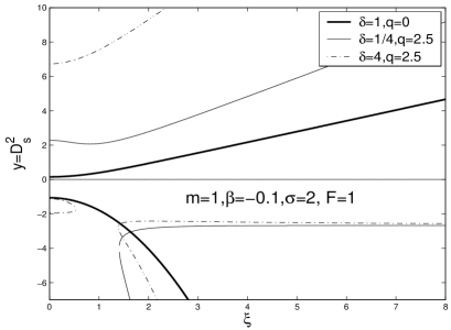
(a) $m=1,\ \beta=-0.1,\ \sigma=2,\ F=1$

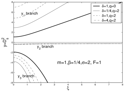
(b) $m=1,\ \beta=1/4,\ \sigma=2,\ F=1$

Figure 15: The $D_{s}^{2}$ solution curves versus $\xi$ for a logarithmic spiral with $m=1$. For $\beta=-0.1$ in panel (a), there can be only one real root and for $\beta=1/4$ in panel (b) the curves are similar to the unmagnetized case. In panel (b), the three curves of $y_{2}$ branch almost overlap with each other.

The $m=1$ case reveals some interesting features to note. We show a few cases in Fig. 15. Here the unmagnetized two solutions of Shen & Lou (2004b) correspond to our $y_{1}$ and $y_{3}$ branches. The $y_{3}$ branch is monotonically decreasing with $\xi$. For a small $\beta$, there can be only one real root and the other two are complex conjugates [see Fig. 15(a)]. We also see that both $q$ and $\delta$ have a strong influence on the solution behaviours. For the physical $y_{1}$ solution branch, a strong magnetic field as well as a high $\delta$ greatly raises the solution curves.

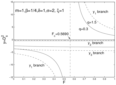
(a) $m=1,\ \beta=1/4,\ \delta=1,\ \sigma=2,\ \xi=1$, $q=0.3$ (solid curves) and $1.5$ (dashed curve)

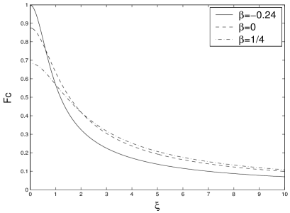
(b) Critical value of $F_{c}$ versus $\xi$ for the case $m=1$ with three different $\beta$ values.

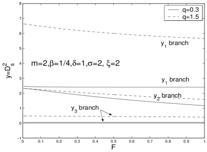
(c) $m=2,\ \beta=1/4,\ \delta=1,\ \sigma=2,\ \xi=2$, $q=0.3$ (solid curves) and $1.5$ (dashed curve)

Figure 16: Solutions for a composite system of partial scale-free discs. For $m=1$ cases, there exists $F_{c}$ such that the $y_{1}$ solution diverges [see panel (a)]. This $F_{c}$ depends only on $\beta$ and $\xi$ as shown in panel (b). For $m\geq 2$ cases, the ratio $F$ does not have much influence on the behaviour of $D_{s}^{2}$ solutions.

For a composite system of two partial scale-free discs embedded in an axisymmetric dark matter halo, we distinguish $m=1$ and $m>1$ cases. In the $m=1$ case, there always exists the critical value $F_{c}$ for the potential ratio $F$ parameter such that the $y_{1}$ solution branch diverges from either side of $F_{c}$. Mathematically, this critical value $F_{c}$ is determined by $C^{S}_{3}=0$ and is quite similar to that in the aligned cases. For $F\leq F_{c}$, there is no physical solution, while for $F>F_{c}$ the $y_{1}$ branch is physical and sensitive to $F$ variation; the existence of an axisymmetric dark matter halo can significantly influence global configurations in a composite disc system with $m=1$ MHD perturbations. Here $F_{c}$ depends only on $\beta$ and $\xi$ and we demonstrate this dependence using examples in Fig. 16(b). The $F_{c}$ curves with different $\beta$ decrease monotonically as $\xi$ increases. For a small radial wavenumber $\xi\leq 1$, the critical value $F_{c}$ approaches 1 as seen in panels (a) and (b) of Fig. 16. Since in reality the dark matter halos play significant roles in disc galaxies (i.e., $F$ is small and not close to 1), we propose that a spiral galaxy with only one spiral arm with a relatively large proportion of dark matter halo must have a relatively large radial wavenumber (i.e., tightly wound) to support a global stationary pattern. In principle, this may be tested by observations.

For spiral perturbations with $m>1$, however, the dark matter seems to be less important in determining the stationary dispersion relation. Because in the entire range of $0<F\leq 1$, there are only slight variations in the $D_{s}^{2}$ solutions. We show such an example in Fig. 16(c). With a radial wavenumber $\xi=2$, all three solution branches $y_{1}$, $y_{2}$ and $y_{3}$ remain positive and rise only slightly as $F$ decreases. We can also compare Fig. 12(a) and Fig. 12(c), Fig. 14(a) and Fig. 14(c) and see that in $m=2$ cases, the dark matter halo has little influence on solutions. For cases of $m\geq 3$, the situations are qualitatively similar. Nevertheless, a dark matter halo should have a strong stabilizing effect in general.

4.2.3 Phase Relationships among Perturbation Variables

For logarithmic spiral cases, the phase relationships among coplanar MHD perturbation variables have more features to explore. The introduction of radial oscillations with radial wavenumber $\xi$ brings an imaginary part into our equations which describes the phase difference between perturbed surface mass density and the magnetic field perturbation as well as other perturbation variables. To describe these phase relations more specifically, we begin with equations $(\ref{eq:82})-(\ref{eq:84})$ to obtain

$$\begin{split}&{S^{g}}/{S^{s}}=-1-\mathcal{M}_{S}/(2\pi G\Sigma_{0}^{s}r\mathcal{N}_{m})\ ,\\ &\frac{\mathrm{i}R}{S^{g}}=\frac{mB_{0}}{\Sigma_{0}^{g}}\bigg{[}\Theta_{S}\bigg{(}1+\frac{S^{s}}{S^{g}}\bigg{)}+\Xi_{S}\bigg{]}\ ,\\ &Z=\xi\mathrm{i}R/m\ .\end{split}$$ (92)

There is another independent expression of $\mathrm{i}R/S^{g}$ obtained by a combination of equations (78) and (79), namely

$$\frac{\mathrm{i}R}{S^{g}}=\frac{mB_{0}}{\Sigma_{0}^{g}}\bigg{[}\frac{(1-2\mathrm{i}\xi)\pi G\Sigma_{0}^{g}r\mathcal{N}_{m}}{\mathcal{K}_{S}}\bigg{(}1+\frac{S^{s}}{S^{g}}\bigg{)}-\frac{\mathcal{L}_{S}}{\mathcal{K}_{S}}\bigg{]}\ .$$ (93)

It is no wonder that these expressions are quite similar to the aligned phase relationships. We next express these results in physical parameters. As $\mathrm{i}R/S^{g}$ is no longer dimensionless, we take the proportional factor in brackets of equation (92). The results are

$$\begin{split}&\frac{S^{g}}{S^{s}}=-1-\frac{(\mathcal{B}_{m}D_{s}^{2}-\mathcal{A}^{S}_{m})}{(D_{s}^{2}+1)}\frac{\mathcal{C}(1+\delta)}{\mathcal{N}_{m}\mathcal{A}^{S}_{m}}\ ,\\ &\frac{\mathrm{i}R}{S^{g}}\propto\frac{m}{(1+2\beta)(3/2-\mathrm{i}\xi)D_{g}^{2}-(1/2-2\beta)q^{2}}\bigg{[}(1+2\beta)D_{g}^{2}\\ &+\frac{D_{g}^{2}+1+{(4\beta-1)q^{2}}/{(4\beta+2)}}{\mathcal{C}(1+\delta)}\bigg{(}1+\frac{S^{s}}{S^{g}}\bigg{)}\mathcal{N}_{m}\delta-1\bigg{]}\ .\end{split}$$ (94)

Since $\mathrm{i}R/S^{g}$ contains imaginary part, the phase difference between surface perturbation mass density and the perturbed magnetic field becomes complicated. For this reason, we show such phase relations in special figures.

We first quickly note that when $q=0$ (unmagnetized) and $\sigma=1$ (the same ‘sound speeds’), the ratio $S^{g}/S^{s}=\pm 1$ for the $y_{1}$ and $y_{2}$ solution branches, respectively. We can prove this claim by using the fact that $y_{1}=\mathcal{A}_{m}/\mathcal{B}_{m}$ and $y_{2}=(1-\mathcal{N}_{m}/\mathcal{C})\mathcal{A}_{m}/\mathcal{H}_{m}$ for the two $D_{s}^{2}$ solutions (Shen & Lou, 2004b) and by substituting these explicit $y_{1}$ and $y_{2}$ expressions into equation (94). For fairly arbitrary parameters, the tendency of the phase relation curves for the ratio of the perturbed surface mass densities in the two scale-free discs are shown in Fig. 17 and Fig. 18. We would emphasize that the relative order of the three branches varies in the phase relation curves. For example, for a small $\beta=-0.24$, the $y_{3}$ branch is the lowest, while for a larger $\beta=1/4$, it becomes the upper one.

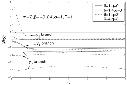
(a) $m=2,\ \beta=-0.24,\ \sigma=1,\ F=1$

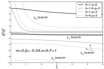
(b) $m=2,\ \beta=-0.24,\ \sigma=5,\ F=1$

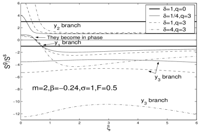
(c) $m=2,\ \beta=-0.24,\ \sigma=1,\ F=0.5$

Figure 17: Phase relation curves for the ratio $S^{g}/S^{s}$ of surface mass density perturbation versus the radial wave number $\xi$ for the case of $m=2$ and $\beta=-0.24$. The solutions with $q=3,\ \delta=1/4,\ 1$ and $4$ are shown in light solid curve, dashed curve and dash-dotted curve, respectively. We examine full discs ($F=1$) with $\sigma=1$ and $\sigma=5$ in panels (a) and (b), respectively. For a partial disc with $F=0.5$, we show solutions with $\sigma=1$ in panel (c). In all panels, the solution branches $y_{1}$, $y_{2}$, and $y_{3}$ can be readily identified. Each branch contains three distinct solutions with $\delta=1/4$ (solid curve), 1 (dashed curve) and 4 (dash-dotted curve), respectively. In each panel, the two boldface curves for $y_{1}$ and $y_{2}$ branches correspond to $q=0$ (the $y_{3}$ branch is trivial).

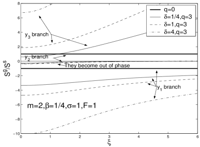
(a) $m=2,\ \beta=1/4,\ \sigma=1,\ F=1$

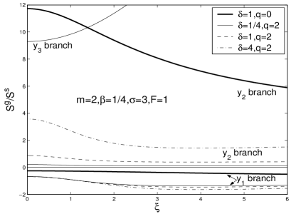
(b) $m=2,\ \beta=1/4,\ \sigma=3,\ F=1$

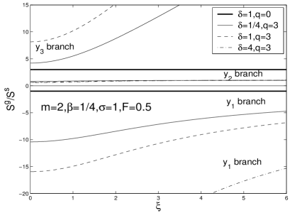
(c) $m=2,\ \beta=1/4,\ \sigma=1,\ F=0.5$

Figure 18: The phase relation curves for the ratio $S^{g}/S^{s}$ of surface mass density perturbations versus $\xi$ for a logarithmic spiral case with $m=2$ and $\beta=1/4$. We show separately phase curves for full discs ($F=1$) with $\sigma=1$ and $\sigma=3$ in panels (a) and (b), respectively. For a partial disc of $F=0.5$ with $\sigma=1$, we show solution branches in panel (c). Note that in the case $q=0$ (boldface curves) and $\sigma=1$, the two solution branches have $S^{g}/S^{s}=\pm 1$ [see equation (73) of Shen & Lou (2004b)].

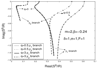
(a) $m=2,\ \beta=-0.24,\ \delta=1,\ \sigma=1,\ F=1$

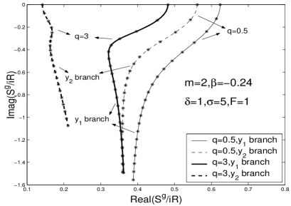
(b) $m=2,\ \beta=-0.24,\ \delta=1,\ \sigma=5,\ F=1$

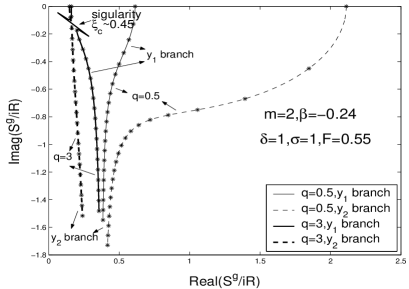
(c) $m=2,\ \beta=-0.24,\ \delta=1,\ \sigma=1,\ F=0.5$

Figure 19: The phase relation curves for the perturbed radial magnetic field and gas surface mass density versus $\xi$ for the case of $m=2$ and $\beta=-0.24$. The ratio $S^{g}/(\mathrm{i}R)$ is generally complex and is shown here in the complex plane with real and imaginary axes. We take the range of $\xi=0$ to 6. For $\xi=0$, the imaginary part is zero according to equation (94). As $\xi$ grows, the imaginary part emerges and becomes more significant. To demonstrate the relation with $\xi$, we show $*$ to mark an interval of 0.3 in the variation of $\xi$ from $0$ to $6$. In this case, only the $y_{1}$ and $y_{2}$ solution branches are physical and the unphysical $y_{3}$ branch is ignored.

In the case of $\beta=-0.24$ and for full discs, the phase relation of the perturbed surface mass densities in the two scale-free discs is out of phase for the $y_{1}$ branch and in phase for the $y_{2}$ branch ($y_{3}$ branch is unphysical) even with a strong magnetic field; this situation differs from the aligned cases. For the $y_{2}$ branch in full discs, a small $\xi$ leads to a larger $S^{g}/S^{s}$ ratio, while for a large $\xi$, the ratio can be rather small compared with $\delta$. For the $y_{1}$ branch in full discs, the $S^{g}/S^{s}$ curves with different $\delta$ values do not vary significantly. For a small $\xi$, the ratio $|S^{g}/S^{s}|$ is fairly small and for a large $\xi$, this ratio lies between 1 and 2. The increase of $\sigma$ generally raises the two branches to different levels. The presence of magnetic field gives rise to variations in the $y_{1}$ solution curves in two trends: the curves move above and below the $q=0$ solution curve for small and large $\xi$, respectively (see Fig. 17). For a composite system of two coupled partial scale-free discs, some of these tendencies does not hold. First, $S^{g}/S^{s}$ may become positive for the $y_{1}$ branch with a sufficiently small radial wavenumber $\xi$. It also raises the $y_{2}$ branch considerably and separates solutions of $y_{1}$ branch with different $\delta$ values. In other words, the influence of $\delta$ becomes more prominent.

In the case of $\beta=1/4$, the phase relation curves of the perturbed surface mass densities for the $y_{1}$ solution branch remain negative. For small $\sigma$, variations of $\delta$ produce considerable differences in phase curves, while for large $\sigma$, phase curves with various $\delta$ values become much closer. For the $y_{2}$ branch with a small $\sigma$, the ratio $S^{g}/S^{s}$ can become negative at a certain $\sigma_{c}$ with $S^{g}=0$ and the curves with different $\delta$ values are bunched together. For a large $\sigma$, the ratio $S^{g}/S^{s}$ are positive and the curves with different $\delta$ values are separated. In the case of a small $\sigma=1$, the $y_{3}$ branch is physical with a positive $S^{g}/S^{s}$ ratio growing with $\xi$. The value of $\delta$ influences the phase relation in this branch in a significant manner. In a composite system of partial discs, the presence of a dark matter halo raises the $y_{2}$ and $y_{3}$ solution branches and lowers the $y_{1}$ solution branch in the phase relation curve. Meanwhile, the $S^{g}/S^{s}$ ratio is positive for the $y_{2}$ branch, and for the $y_{1}$ and $y_{3}$ branches, the ratio magnitude $|S^{g}/S^{s}|$ becomes much larger than that for a composite system of full discs.

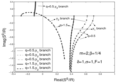
(a) $m=2,\ \beta=1/4,\ \delta=1,\ \sigma=1,\ F=1$

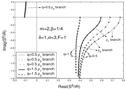
(b) $m=2,\ \beta=1/4,\ \delta=1,\ \sigma=3,\ F=1$

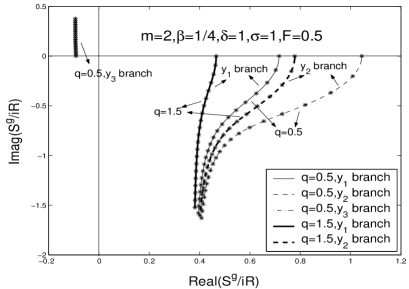
(c) $m=2,\ \beta=1/4,\ \delta=1,\ \sigma=1,\ F=0.5$

Figure 20: The phase relation curves for real and imaginary parts of $S^{g}/(\mathrm{i}R)$ between the radial component of the perturbation magnetic field and surface mass density versus $\xi$ for logarithmic spirals with $m=2$ and $\beta=1/4$ in a complex plane. We show separately curves of full discs ($F=1$) with $\sigma=1$ and $\sigma=3$ in panels (a) and (b), respectively, and for a partial disc with $\sigma=1$ in panel (c). We also add the phase curve for the physical $y_{3}$ branch. When $q=1.5$, the $y_{3}$ branch is very far away from the other curves; we have omitted this curve for the compactness of presentation.

We now examine the phase relationship between the perturbed gas surface mass density and the perturbed magnetic field as these aspects may provide useful diagnostics for observations. Since both $S^{g}/(\mathrm{i}R)$ and $S^{g}/Z$ are complex in general, we show such phase relation in the complex plane. In Fig. 19 and Fig. 20 for the complex ratio $S^{g}/(\mathrm{i}R)$, the variation of $\xi$ is labelled by an asterisk $*$ with an interval of $\Delta\xi=0.3$ starting from the real axis. According to equation (94), the $S^{g}/(\mathrm{i}R)$ ratio is real for $\xi=0$ and thus the curves start from the real axis. In Fig. 21 and Fig. 22 for $S^{g}/Z$, the variation of $\xi$ is labelled by an asterisk $*$ with an interval of $\Delta\xi=0.4$. According to equation (92), $S^{g}/Z\rightarrow\infty$ as $\xi\rightarrow 0$. Equation (92) also tells us that the phase relations of the azimuthal magnetic field perturbation and the gas surface mass density are totally opposite for leading ($\xi>0$) and trailing ($\xi<0$) spiral MHD density waves.

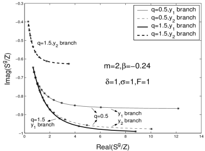
(a) $m=2,\ \beta=1/4,\ \delta=1,\ \sigma=1,\ F=1$

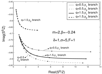
(b) $m=2,\ \beta=1/4,\ \delta=1,\ \sigma=3,\ F=1$

Figure 21: The phase relation curves between the perturbed azimuthal magnetic field and surface mass density versus $\sigma$ for logarithmic spirals with $m=2,\ \beta=-0.24$. We show curves of full discs ($F=1$) with $\sigma=1$ and $\sigma=3$ in panels (a) and (b). We take the range of $\xi=0.4$ to 4. Since $S^{g}/Z\rightarrow\infty$ as $\xi\rightarrow 0$, we start from $\xi=0.4$ and use $*$ to label an interval of 0.4 in the variation of $\xi$. The phase points moves from right to left as $\xi$ increases.

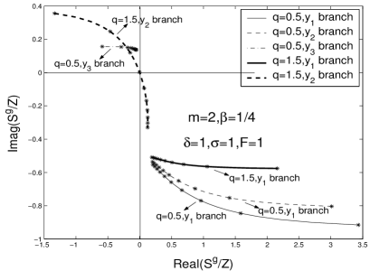
(a) $m=2,\ \beta=1/4,\ \delta=1,\ \sigma=1,\ F=1$

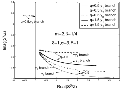
(b) $m=2,\ \beta=1/4,\ \delta=1,\ \sigma=3,\ F=1$

Figure 22: The phase relation curves between the perturbed azimuthal magnetic field and surface mass density versus $\sigma$ for logarithmic spirals with $m=2,\ \beta=1/4$. We show curves of full discs ($F=1$) with $\sigma=1$ and $\sigma=3$ in panels (a) and (b). We also add the physical $y_{3}$ branch. When $q=1.5$, the $y_{3}$ branch is very far away from the other curves and we have omitted this curve for the compactness of presentation. We start from $\xi=0.4$ and use $*$ to label an interval of 0.4 in the variation of $\xi$. The phase points moves from right to left for the $y_{1}$ and $y_{2}$ branches and from left to right for the $y_{3}$ branch as $\xi$ increases.

In the case of $\beta=-0.24$, only the $y_{1}$ and $y_{2}$ branches are physical, and we show these two branches in Fig. 19 and Fig. 21. The main trend is that with the increase of the radial wavenumber $\xi$, the real part of $S^{g}/(\mathrm{i}R)$ is positive and does not vary much as the imaginary part decreases steadily from zero. The result is that for tight-winding spiral arms with large $\xi$, the radial component of the magnetic field perturbation becomes almost in phase with the gas density perturbation (i.e., $S^{g}/R\rightarrow$ a positive number), while for a small $\xi$, the radial component of the magnetic field perturbation lags behind the perturbed gas density by $\sim\pi/2$, a trend similar to the aligned cases. The azimuthal component of the magnetic field perturbation $Z=\xi\mathrm{i}R/m$ remains always ahead of the radial component of the magnetic field perturbation by $\pi/2$ in phase. We note that for small $\xi$ the imaginary part of $S^{g}/Z$ approaches a constant as its real part moves to infinity. Meanwhile, the azimuthal magnetic field perturbation can be much larger than the radial magnetic field perturbation for large $\xi$. For a composite system of partial scale-free discs with a coplanar magnetic field, we note the following two points. First, by decreasing the potential parameter $F$, the $y_{2}$ branch moves towards right while the $y_{1}$ branch does not move much. Secondly, for a large magnetic parameter $q=3$, singularity occurs in the $y_{1}$ branch as $F$ decreases. This singularity can be determined from equation (94), namely

$$\begin{split}\frac{[D_{g}^{2}+1+(4\beta-1)q^{2}/(4\beta+2)]\mathcal{N}_{m}\delta}{\mathcal{C}(1+\delta)}\bigg{(}1+\frac{S^{s}}{S^{g}}\bigg{)}\qquad\\ \qquad-1+(1+2\beta)D_{g}^{2}=0\ ,\end{split}$$ (95)

where $F$ parameter is implicitly contained in coefficient $\mathcal{C}$.

The $y_{3}$ branch can be positive in the case of $\beta=1/4$ (see Fig. 14 for this SMDW mode); we therefore include the phase information of the $y_{3}$ branch in Fig. 20 and Fig. 22. Different from the $y_{1}$ and $y_{2}$ branches, the $y_{3}$ branch has a $S^{g}/(\mathrm{i}R)$ characterized by an almost negative real part and an imaginary part increasing (rather than decreasing) steadily with the increase of $\xi$. The phase relation of this $y_{3}$ branch has a phase difference of $\sim\pi$ relative to the other two branches. For $S^{g}/Z$, the $y_{3}$ branch still lies in the second quadrant and moves from left to right and tends to the upper imaginary axis. It indicates that for this branch the azimuthal magnetic perturbation lags behind the gas surface mass density perturbation by $\sim\pi$ for small $\xi$ and by $\sim\pi/2$ as $\xi$ becomes fairly large. There is yet another salient feature. For a small $\sigma=1$ and a large $q=1.5$, the $y_{2}$ branch appears fairly special. In panel (a) of Fig. 20, starting from a negative real value as $\xi$ increases, the imaginary part first increases and then decreases, meanwhile the real part increases with increasing $\xi$; the curve intersects the real axis again at the origin exactly. It then keeps this tendency such that the imaginary part falls down steadily as $\xi$ increases. In terms of phase difference between $S^{g}$ and $R$ or $S^{g}$ and $Z$, this branch is special in that there is a phase shift of $\pi$ at some $\xi_{c}$. This point corresponds to $S^{g}=0$, also related to the phase shift of $S^{g}/S^{s}$ discussed earlier. For cases of partial discs with $F=0.5$, such ‘singularity’ no longer exists and all curves are continuous. Meanwhile, such $\sim\pi$ phase shift of $y_{2}$ branch in the presence of a strong magnetic field no longer exists either.

4.3 Marginal Stability Curves for
   Axisymmetric Disturbances

The $m=0$ ‘spiral’ case is very special. It is considered as a purely radial oscillation in a composite MHD disc system and is related to part of the MHD disc stability problem. In a general disc problem, the dispersion relation for time-dependent MHD perturbations involves a $\omega^{2}$ term. A linearly stable disc system requires $\omega^{2}\geq 0$. In our analysis, we set $\omega=0$ to obtain stationary patterns and to also meet the requirement of the scale-free condition. In the $m=0$ case, the stationary dispersion relation with $\omega=0$ actually corresponds to the marginal stability curve (Shen & Lou, 2003, 2006, 2004b; Lou & Zou, 2004, 2006). Meanwhile to treat the problem properly, a different limiting process should be taken similar to the aligned $m=0$ case. That is, we first set $m=0$ with $\omega\neq 0$ and then let $\omega\rightarrow 0$ in the relevant MHD perturbation equations. The same as before, we begin with equations $(\ref{eq:48})-(\ref{eq:52})$. Equation (49) requires $U\propto r^{1/2+2\beta+\mathrm{i}\xi}$ and then equation (51) gives $J\propto r^{1/2+\beta+\mathrm{i}\xi}$. Substituting these two expressions into equation (50), we see that the scale-free condition cannot be met unless $\omega=0$ where $U=0$ with $U/\omega\neq 0$. In the process of taking the limit of $\omega\rightarrow 0$, we also remove terms that are not scale free. We show the result of this limiting process below.

$$\begin{split}&r^{2}(\omega^{2}-\kappa_{g}^{2})S^{g}=(\xi^{2}+1/4)\Sigma_{0}^{g}\Psi^{g}+(\xi^{2}+1/4-\beta)C_{A}^{2}S^{g}\ ,\\ &r^{2}(\omega^{2}-\kappa_{s}^{2})S^{g}=(\xi^{2}+1/4)\Sigma_{0}^{s}\Psi^{s}\ .\end{split}$$ (96)

A substitution of equations (36) and (76) into equation (96) with $\omega=0$ yields

$$\begin{split}&[\mathcal{A}^{S^{\prime}}_{0}a_{g}^{2}+\kappa_{g}^{2}r^{2}+(\mathcal{A}^{S^{\prime}}_{0}-\beta)C_{A}^{2}-2\pi Gr\mathcal{A}^{S^{\prime}}_{0}\mathcal{N}_{0}\Sigma_{0}^{g}]S^{g}\\ &\qquad\qquad\qquad\qquad\qquad\qquad-2\pi Gr\mathcal{A}^{S^{\prime}}_{0}\mathcal{N}_{0}\Sigma_{0}^{g}S^{s}=0\ ,\\ &[\mathcal{A}^{S^{\prime}}_{0}a_{s}^{2}+\kappa_{s}^{2}r^{2}-2\pi Gr\mathcal{A}^{S^{\prime}}_{0}\mathcal{N}_{0}\Sigma_{0}^{s}]S^{s}\\ &\qquad\qquad\qquad\qquad\qquad\qquad-2\pi Gr\mathcal{A}^{S^{\prime}}_{0}\mathcal{N}_{0}\Sigma_{0}^{s}S^{g}=0\ ,\\ \end{split}$$ (97)

where we define

$$\mathcal{A}^{S^{\prime}}_{0}\equiv\xi^{2}+1/4$$

and the corresponding notation

$$\mathcal{H}^{S^{\prime}}_{0}\equiv{\mathcal{A}^{S^{\prime}}_{0}\mathcal{N}_{0}}/{\mathcal{C}}+\mathcal{B}_{0}\ .$$

The difference between $\mathcal{A}^{S}_{0}$ and $\mathcal{A}^{S^{\prime}}_{0}$ is that the latter does not contain the term $2\beta$; this is exactly the result of different limiting processes.

The two relations in equation (97) cannot be satisfied unless the coefficient determinant vanishes, which leads to

$$\begin{split}&[\mathcal{A}^{S^{\prime}}_{0}a_{g}^{2}+\kappa_{g}^{2}r^{2}+(\mathcal{A}^{S^{\prime}}_{0}-\beta)C_{A}^{2}-2\pi Gr\mathcal{A}^{S^{\prime}}_{0}\mathcal{N}_{0}\Sigma_{0}^{g}]\\ &\qquad\qquad\times[\mathcal{A}^{S^{\prime}}_{0}a_{s}^{2}+\kappa_{s}^{2}r^{2}-2\pi Gr\mathcal{A}^{S^{\prime}}_{0}\mathcal{N}_{0}\Sigma_{0}^{s}]\\ &\qquad\qquad\qquad\qquad\qquad\qquad=(2\pi Gr\mathcal{A}^{S^{\prime}}_{0}\mathcal{N}_{0})^{2}\Sigma_{0}^{g}\Sigma_{0}^{s}\ .\end{split}$$ (98)

Substitutions of equations $(\ref{eq:20})-(\ref{eq:23})$ lead to the explicit expression of this stationary dispersion relation (98) in terms of physical parameters in the form of

$$\begin{split}&\bigg{\{}\frac{\mathcal{A}^{S^{\prime}}_{0}}{(1+2\beta)}+2(1-\beta)D_{g}^{2}+\frac{q^{2}(\mathcal{A}^{S^{\prime}}_{0}-\beta)}{(1+2\beta)}\\ &-\mathcal{A}^{S^{\prime}}_{0}\mathcal{N}_{0}F\frac{[D_{g}^{2}+1+(4\beta-1)q^{2}/(4\beta+2)]\delta}{2\beta\mathcal{P}_{0}(1+\delta)}\bigg{\}}\\ &\times\bigg{[}\frac{\mathcal{A}^{S^{\prime}}_{0}}{1+2\beta}+2(1-\beta)D_{s}^{2}-\frac{\mathcal{A}^{S^{\prime}}_{0}\mathcal{N}_{0}F(D_{s}^{2}+1)}{2\beta\mathcal{P}_{0}(1+\delta)}\bigg{]}\\ &=\bigg{[}\frac{\mathcal{A}^{S^{\prime}}_{0}\mathcal{N}_{0}F}{2\beta\mathcal{P}_{0}(1+\delta)}\bigg{]}^{2}\bigg{[}D_{g}^{2}+1+\frac{(4\beta-1)q^{2}}{(4\beta+2)}\bigg{]}(D_{s}^{2}+1)\delta\ .\end{split}$$ (99)

By rearranging equation (99), we obtain a quadratic equation for the marginal stability in terms of $y=D_{s}^{2}$, namely

$$C^{M}_{2}y^{2}+C^{M}_{1}y+C^{M}_{0}=0\ ,$$ (100)

where

$$\begin{split}&C^{M}_{2}\equiv\mathcal{B}_{0}\mathcal{H}^{S^{\prime}}_{0}\sigma\ ,\\ &C^{M}_{1}\equiv\bigg{[}(\mathcal{B}_{0}-\mathcal{A}^{S^{\prime}}_{0})\mathcal{H}^{S^{\prime}}_{0}+\frac{(\mathcal{A}^{S^{\prime}}_{0}+\mathcal{B}_{0})(\mathcal{H}^{S^{\prime}}_{0}-\mathcal{B}_{0})}{(1+\delta)}\bigg{]}\sigma\\ &\qquad-\frac{(\mathcal{A}^{S^{\prime}}_{0}+\mathcal{B}_{0})(\mathcal{H}^{S^{\prime}}_{0}+\mathcal{B}_{0}\delta)}{(1+\delta)}\\ &\qquad-\frac{(\mathcal{A}^{S^{\prime}}_{0}+\mathcal{B}_{0}-4\beta+3)(\mathcal{H}^{S^{\prime}}_{0}\delta+\mathcal{B}_{0})}{(1+\delta)}q^{2}\ ,\\ &C^{M}_{0}\equiv\bigg{[}-\mathcal{A}^{S^{\prime}}_{0}\mathcal{H}^{S^{\prime}}_{0}+\frac{(\mathcal{A}^{S^{\prime}}_{0}+\mathcal{B}_{0})(\mathcal{H}^{S^{\prime}}_{0}-\mathcal{B}_{0})}{(1+\delta)}\bigg{]}\sigma\\ &\qquad+(\mathcal{A}^{S^{\prime}}_{0}+\mathcal{B}_{0})\bigg{[}\mathcal{A}^{S^{\prime}}_{0}+\mathcal{B}_{0}-\frac{\mathcal{H}^{S^{\prime}}_{0}+\mathcal{B}_{0}\delta}{1+\delta}\bigg{]}\\ &+(\mathcal{A}^{S^{\prime}}_{0}+\mathcal{B}_{0}-4\beta+3)\bigg{[}\mathcal{A}^{S^{\prime}}_{0}+\mathcal{B}_{0}-\frac{\mathcal{H}^{S^{\prime}}_{0}+\mathcal{B}_{0}\delta}{1+\delta}\bigg{]}q^{2}\ .\\ \end{split}$$ (101)

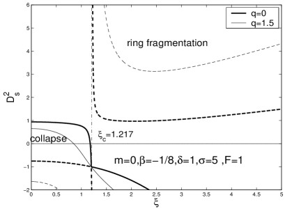
(a) $m=0,\ \beta=-1/8,\ \delta=1,\ \sigma=5,\ F=1$

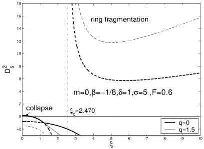
(b) $m=0,\ \beta=-1/8,\ \delta=1,\ \sigma=5,\ F=0.6$

Figure 23: The marginal stability curves for the case of $m=0$, $\beta=-1/8$, $\delta=1$, $\sigma=5$. For comparison, we show the cases $q=0$ (boldface curves) and $q=1.5$ (light curves) in one figure. Note that for a full disc ($F=1$) and a partial disc ($F=0.6$), the marginal stability curves behave quite differently.

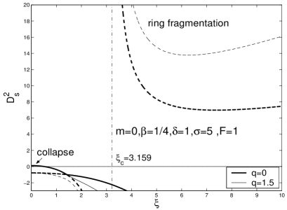
(a) $m=0,\ \beta=1/4,\ \delta=1,\ \sigma=5,\ F=1$

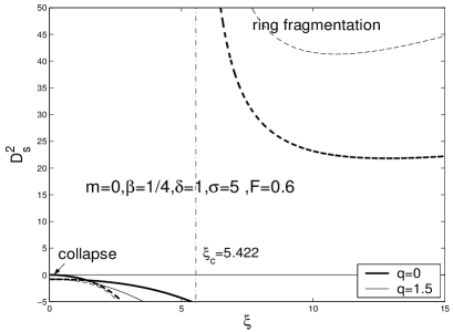
(b) $m=0,\ \beta=1/4,\ \delta=1,\ \sigma=5,\ F=0.6$

Figure 24: The marginal stability curves for the case $m=0$, $\beta=1/4$, $\delta=1$, $\sigma=5$. For both $F=0.6$ and $F=1$, the two cases of $q=0$ and $q=1.5$ are computed. Compared with a smaller $\beta$, the ring fragmentation regions rise up while the MHD Jeans collapse regions shrink.

One necessary check for a consistent derivation is to set $q=0$ and the coefficients (101) reduce to those in the case of unmagnetized coupled scale-free discs (Shen & Lou, 2004b). Equation (100) is quadratic in $D_{s}^{2}$ and has two solution branches corresponding to the marginal stability curves. For several chosen sets of parameters, we demonstrate these $D_{s}^{2}$ curves in Fig. 23 and Fig. 24. The unstable regime consists of two regions. In the upper-right corner, the two coupled discs rotate too fast to be stable and are susceptible to the MHD ring fragmentation instability, while in the lower-left corner the two coupled discs rotate too slow to resist large-scale Jeans collapse modified by rotation and magnetic field (Lemos et al., 1991; Syer & Tremaine, 1996; Shu et al., 2000; Lou, 2002; Lou & Fan, 2002; Lou & Shen, 2003; Lou & Wu, 2005; Shen & Lou, 2004b; Shen et al., 2005; Lou & Zou, 2004, 2006). The marginal curves represent precise global treatments of axisymmetric linear stability. In the WKBJ or tight-winding regime, one can readily derive the local dispersion relation for a single MHD disc and the local dispersion relation for a composite system of gravitationally coupled discs in the WKBJ regime can be expressed in a parallel form as equation (98). As discussed for a single scale-free MHD disc by Shen et al. (2005), the WKBJ approximation is well justified for short wavelength perturbations (i.e., large $\xi$) but not as good for long wavelength perturbations.

We comment on the MHD ring fragmentation instability here. In fact, this is the MHD generalization of the well-known Toomre instability characterized by the so-called $Q$ parameter (Safronov, 1960; Toomre, 1964). Besides in contexts of single discs, there have been numerous studies to identify such an effective $Q$ parameter for a composite disc system (Elmegreen, 1995; Jog, 1996; Lou & Fan, 1998b) and in a single coplanar magnetized SID (Lou & Fan, 1998a). Shu et al. (2000) noted that in a single SID, the minimum of the ring fragmentation branch is effectively related to the Toomre $Q$ parameter. For a coplanar magnetized SID, Lou (2002) and Lou & Fan (2002) emphasized that the MHD ring fragmentation branch is also closely related to the generalized $Q_{M}$ parameter (Lou & Fan, 1998a). The conceptual connection of two instabilities comes from their dependence on radial wavenumber. Physically, Shen & Lou (2003) suggested a straightforward $D$ criterion to determine the axisymmetric stability against ring fragmentation. In our composite scale-free discs with a coplanar magnetic field, we therefore interpret this MHD ring fragmentation as an extension of the Toomre instability, with $D_{s}$ parameter being used for the stability criterion. In addition, this $D_{s}$ parameter describes a global MHD instability criterion, while the $Q$ parameter is only defined locally.

When $C_{2}^{M}=0$ occurs for $\xi=\xi_{c}$, one branch of the stability curves diverges at $\xi=\xi_{c}$. For a specified $\beta$ value, the divergent point $\xi_{c}$ depends only on $F$ parameter contained in the coefficient $\mathcal{C}$.

For hydrodynamic perturbations in coupled scale-free discs without magnetic field, Shen & Lou (2004b) have discussed the results thoroughly and their figures clearly show the influence of the two parameters $\sigma$ and $\delta$ (see their Fig. 4 to Fig. 8), for example, the increase of $\sigma$ or $\delta$ lowers both the collapse and ring fragmentation regions. In other words, the increase of $\sigma$ or $\delta$ reduces the danger of the Jeans collapse instability but makes the composite system more vulnerable to the ring fragmentation instability. By our exploration in the presence of magnetic field, this trend of variation remains. For this reason, we shall not repeat the analysis in this regard similar to theirs. We mainly focus on the case of $\delta=1,\ \sigma=5$ and show the marginal stability curves for $q=0$ and $q=1.5$ in one figure. Similar to the study of Shen et al. (2005) where global coplanar MHD perturbation structures in a single scale-free gaseous disc with a coplanar magnetic field are analyzed, we arrive at the same conclusion in our model of a composite system of coupled scale-free discs. The enhancement of a coplanar magnetic field reduces the danger of ring fragmentation in an apparent manner; and at the same time, it only suppresses Jeans collapse instabilities for the $\beta$ range of $-1/4<\beta<1/4$ and tends to aggravate Jeans collapse instabilities for the $\beta$ range of $1/4<\beta<1/2$. As has been already mentioned in Shen et al. (2005), this collapse feature can be understood from the coupling between the surface mass density and the coplanar magnetic field of the background rotational MHD equilibrium.

We also examine global MHD perturbation structures in a composite system of partial scale-free discs with the potential factor $F=0.6$. It is clear from Fig. 23 and Fig. 24 that the presence of an axisymmetric dark matter halo suppresses both the ring fragmentation and Jeans collapse instabilities. This results from the fact that the dark matter halo exists as a stationary massive gravitational background. It can reduce the ring fragmentation because its gravitational force acts as centripetal force to resist such danger. It can suppress Jeans collapse because its stationary background supports the stationary structure of the discs (Miller et al., 1970; Hohl, 1971; Ostriker & Peebles, 1973; Binney & Tremaine, 1987).

5 Summary and discussion

From several perspectives, this paper represents a generalization and extension of previous works [Syer & Tremaine (1996); Shu et al. (2000); Kalnajs (1971); Lou (2002); Lou & Fan (2002); Lou & Wu (2005); Lou & Zou (2004, 2006); Shen & Lou (2004b); Shen et al. (2005)]. We consider a composite disc system consisting of gravitationally coupled stellar and gas scale-free discs with a coplanar magnetic field and construct global stationary coplanar MHD perturbation structures within such a composite disc system. More specifically, such discs are treated as razor-thin and scale-free so that the entire problem is two-dimensional with all background quantities varying in power laws of radius $r$. For the background rotational MHD equilibrium, the surface mass density scales as $\Sigma_{0}\propto r^{-\alpha}$, the rotation curve scales as $v_{0}\propto r^{-\beta}$ and the azimuthal magnetic field scales as $B_{0}\propto r^{-\gamma}$. The barotropic equation of state is expressed as $\Pi=K\Sigma^{n}$. By the scale-free condition, the indices $\alpha,\ \beta,\ \gamma,\ n$ are all expressed in terms of $\beta$ by equation (19). The two discs are gravitationally coupled through the Poisson integral and the scale-free condition requires that the physical quantities of the two discs should share the same radial scalings with different proportional coefficients allowed. Meanwhile, the potential factor $F$ for a composite partial disc system is included to represent the ratio of the gravitational potential arising from the composite disc system to that arising from the entire system including a massive axisymmetric dark matter halo mass distribution which is assumed unresponsive to perturbations in the composite disc system. For convenience and clarity, several dimensionless constant parameters are introduced. The first one is the effective rotational Mach number $D$ (we omit either subscript or superscript ‘$g$’ or ‘$s$’ for simplicity here) defined as the ratio of the disc rotation speed to the disc sound speed yet with an additional scaling factor $(1+2\beta)^{-1/2}$. In essence, this is a measure for the disc rotational velocity. The second one is $q$ parameter corresponding to the ratio of the Alfvén wave speed to the gas sound speed which provides a measure for the strength of the coplanar magnetic field. The other two parameters are $\delta$ and $\eta$ which represent the ratio of surface mass densities of the two discs and the square of the sound speed ratio (the velocity dispersion in the stellar disc mimics the sound speed in our formulation) of the two discs, respectively. For the convenience of figure presentation, we also define $\sigma\equiv 1/\eta$. These parameters completely characterize the behaviour of a composite disc system for the background equilibrium and are independent of each other; to a greater extent, they can be freely chosen but within a certain bound. In our model, there is a wide range of freedom to choose these parameters. Our goal is to study stationary coplanar MHD perturbations to construct global aligned and unaligned configurations described by the relevant dispersion relations containing all these parameters and to analyze partially the linear instability problem of such a composite disc system.

Our model is highly idealized in several aspects, nevertheless, these simplifications are sensible and useful in making the problem tractable. First, we adopt the razor-thin approximation for the composite disc system so that vertical variations across the disc system are ignored [e.g., Qian (1992); Syer & Tremaine (1996); Fan & Lou (1997); Shu et al. (2000); Lou & Fan (1998b)]. This is justifiable so long as the radial scale of a galactic disc is much larger than the disc thickness. Secondly, we simplify a galactic system to just three major constituent components: a magnetized gas disc, a stellar disc (treated as a fluid) and an axisymmetric dark matter halo. In reality, there exists another component of cosmic rays, important from the diagnostic perspective for observing large-scale radio structures as revealed by synchrotron emissions from relativistic electrons gyrating around the galactic magnetic field (Lou & Fan, 2003). Technically, we need to deal with subsystems in a piece-wise manner and different subsystems will manifest different aspects of the physical problem. In our model formalism, we mainly focus on the magnetized interstellar gases and the stars in a galactic disc system in the presence of an axisymmetric dark matter halo. This is typical for disc galaxies including our own Milky-Way. Thirdly, we adopt a simple fluid description for both the stellar and magnetized gas discs. In principle, a distribution function approach to the stellar disc would be more accurate and comprehensive. However, for a large-scale dynamics without resonances etc., a fluid approximation suffices (Lin & Shu, 1964; Binney & Tremaine, 1987; Bertin & Romeo, 1988; Lou & Shen, 2003; Lou & Zou, 2004; Shen & Lou, 2004b). Fourthly, the basic problem is formulated here within the scale-free framework. Now all quantities are required to vary with power-law scalings in $r$, and the barotropic equation of state must be imposed [e.g., Syer & Tremaine (1996); Shen & Lou (2004b); Shen et al. (2005)]. The scale-free condition further requires that the two coupled discs share the same radial scalings as well as the same barotropic index [e.g., Shen & Lou (2004b)]. Another major constraint is that such scale-free configurations must be stationary with $\omega=0$ [e.g., Lou (2002); Lou & Fan (2002); Lou & Shen (2003); Lou & Wu (2005); Lou & Zou (2004, 2006); Shen & Lou (2004b); Shen et al. (2005)]. Nevertheless, the model of coupled scale-free discs represents a significant extension of isothermal discs with $\beta=0$. In particular, global MHD perturbation structures can be constructed with the relevant MHD dispersion relations determined analytically. Fifthly, the background magnetic field is presumed to be azimuthal and bears a radial power-law scaling $r^{-\gamma}$. As the magnetic field distribution in disc galaxies is generally complex, either the isopedic or the coplanar magnetic field geometry represents an idealization. Model analysis in terms of these two ‘orthogonal’ geometries provide a theoretical basis for physical intuitions about magnetic field effects. Our current model focuses on the case of a coplanar magnetic field, while for the case of an isopedic magnetic field, the interested reader is referred to Shu et al. (2000); Lou & Wu (2005) and Wu & Lou (2006).

Our model makes advances in the research in the MHD disc problem. By including two coupled scale-free discs with a coplanar magnetic field, our model contains various model ingredients of previous models of Syer & Tremaine (1996); Shu et al. (2000); Lou (2002); Lou & Fan (2002); Lou & Zou (2004, 2006); Shen & Lou (2004b); Shen et al. (2005). In a fluid-magnetofluid composite disc system with a coplanar magnetic field, we construct both aligned and spiral global MHD perturbation configurations and they are in accordance with previous works and meanwhile there are several new features in our model. With such an analysis, the MHD dispersion relations are derived analytically without any approximation, meanwhile, the axisymmetric marginal stability criteria is also obtained analytically. Our model provides a new perspective for understanding large-scale MHD structures in disc galaxies. We now summarize the main results in the following.

(i) Aligned Stationary MHD Configurations

For the aligned cases, we derive the MHD dispersion relation and provide ample numerical examples concerning global MHD perturbation configurations and the corresponding phase relations among perturbation variables. In our fluid-magnetofluid model of two coupled scale-free discs, the MHD dispersion relation is a cubic equation in terms of $y=D_{s}^{2}$ and there are three $y=D_{s}^{2}$ solution branches in general. By our analysis, the existence of the three branches is due to the gravitational coupling of perturbations in the two discs and the interaction of the magnetic field with the disc system [see the dispersion relation of equation (65)] and they correspond to purely azimuthal propagation of super fast MHD density waves (sFMDWs), fast MHD density waves (FMDWs) and slow MHD density waves (SMDWs), respectively. Generally speaking, the $y_{1}$ branch (sFMDW) is always positive and the $y_{3}$ branch (SMDW) is more often negative thus unphysical. Our interest lies mainly on the $m=2$ (i.e., bar-like) case and we discuss the influence of several parameters.

The magnetic field serves as a centripetal force when $\beta<1/4$ (i.e., magnetic tension force is stronger than the magnetic pressure force) and as a centrifugal force when $\beta>1/4$ (i.e., magnetic tension force is weaker than the magnetic pressure force) for the background MHD rotational equilibrium state. In the presence of coplanar MHD perturbations, there is a gravitational interaction between the two discs and there are also MHD interactions within the magnetized gas disc. For cases of $q^{2}\ll 1$, the magnetic field has very weak influence on the composite disc system. The $y_{3}$ branch becomes trivial. Our $y_{1}$ and $y_{2}$ branches correspond to solutions of Shen & Lou (2004b). While for $q\geq 1$ (i.e., the Alfvén wave speed is comparable to or larger than the sound speed in the gas disc), the behaviour of solution branches can be totally different from the unmagnetized cases of Shen & Lou (2004b) and magnetic field effect can become dominant, especially for small $\sigma$ (e.g., $\sigma\sim 1$). In the presence of magnetic field, we observe a new feature that as $\beta$ and $q$ become large enough, there appears a ‘convergent point’ where for different $\delta$ values some solution branches converge and then their relative positions are changed. Under the assumption that $\eta\leq 1$ (or $\sigma\geq 1$, the gas sound speed is less than the velocity dispersion of the stellar disc) and when $\beta<1/4$, we have $D_{s}<D_{g}$ according to equation (22); the magnetized gas disc rotates faster and the existence of magnetic field enlarges the rotational speed difference between the gas and stellar discs. Yet for a relatively strong magnetic field and for $\beta>1/4$, there are solutions with $D_{s}>D_{g}$ and the stellar disc rotates faster instead (see Fig. 4).

In the aligned cases, the phase relations among perturbation variables are relatively simple because all quantities are real and they must be either in phase or out of phase. For the $y_{1}$ branch, the perturbation mass densities in the two discs are always out of phase while for the other two branches $y_{2}$ and $y_{3}$, the perturbation mass densities are generally in phase. However for the $y_{2}$ branch with a strong magnetic field, the perturbation mass densities can also become out of phase. For the radial component of the magnetic field perturbation, $\mathrm{i}R$ and $S^{g}$ are always in phase for the $y_{1}$ branch; they are in phase for the $y_{2}$ branch and out of phase for the $y_{3}$ branch in many cases but on the whole this phase relation depend on both $q$ and $\sigma$ parameters (see Fig. 10). Since $Z=(4\beta-1)\mathrm{i}R/2m$, the phase relation between gas mass density perturbation and the azimuthal component of the magnetic field perturbation is similar to that of $S^{g}$ and $\mathrm{i}R$ when $\beta>1/4$ and has an additional phase shift $\pi$ for $\beta<1/4$. When $\beta=1/4$ there is no azimuthal magnetic field perturbation.

We also note that when $\beta$ becomes sufficiently small (e.g., $\beta=-0.24$) with a mild magnetic field strength, there exists only one solution branch and the other two are complex conjugates.

Regarding $m$ dependence, there are not many new features except for $m=1$. In this case, the solutions are quite different from $m=2$ modes. In particular, it is now possible that the solution branches intersect and also there can be no physical $D_{s}^{2}$ solutions.

(ii)Stationary Configurations of Logarithmic Spirals

The MHD dispersion relation for the spiral cases is quite similar to that for the aligned cases in form. Differences only occur by a systematic replacement of notations. Therefore, there are many common features in solution behaviours. Physically, logarithmic spirals involve both radial and azimuthal propagations of MHD density waves, while the aligned cases involve purely azimuthal propagations of MHD density waves (Lou, 2002).

In the $m=2$ case, the $y_{3}$ branch is due to the existence of magnetic field and seems to bear little relation with the spiral pattern (i.e., it almost does not vary much for arbitrary $\xi$). This SMDW is in most cases negative thus unphysical. Those physical SMDWs in the spiral cases appear when $\beta$ is not too small (i.e., $\beta\geq 0$) and $\sigma$ is small enough (i.e., $\sigma=1$). The $y_{1}$ and $y_{2}$ solution branches are monotonically increasing with radial wavenumber $\xi$, suggesting that to maintain a stationary tight-winding logarithmic spiral pattern, a fast disc rotation speed is required for sFMDWs or FMDWs. The increase of the magnetic field strength generally raises the solution branches, while a large $\sigma$ tends to lower the solution branches. The ‘convergent point’ appears more often in the logarithmic spiral cases as $\xi$ varies.

We now describe the phase relations among perturbation variables for logarithmic spirals. The phase relation between perturbation surface mass densities remain either in phase or out of phase, and the behaviour is similar to those in the aligned cases, but the phase relation between surface mass density perturbation and the magnetic field perturbation becomes fairly involved. The dependence of $S^{g}/(\mathrm{i}R)$ and $S^{g}/Z$ on $\xi$ is described by a complex expression. Now the azimuthal magnetic field perturbation is $Z=\xi\mathrm{i}R/m$ which is quite different from that of the aligned cases and is dependent on the sign of $\xi$ (i.e., for leading waves and trailing waves the azimuthal magnetic perturbation have a phase difference of $\pi$). In the case of $\xi=0$ for $y_{1}$ and most of $y_{2}$ branches, the ratio $S^{g}/(\mathrm{i}R)$ is positive, i.e., the radial magnetic field perturbation lags behind the gas surface mass density perturbation by $\pi/2$ in phase (no azimuthal magnetic perturbation). As $\xi$ increases, the imaginary part of this ratio decreases in general while its real part does not vary significantly, which indicates that the phase of the radial magnetic field perturbation is catching up with the gas surface mass density perturbation (meanwhile the azimuthal magnetic perturbation becomes ahead of $S^{g}$ from the original in-phase relation). In the tight-winding approximation (i.e., $\xi\rightarrow\infty$), $R$ and $S^{g}$ are in phase and the phase of azimuthal magnetic perturbation tends to be $\sim\pi/2$ ahead of $S^{g}$. We also find that in the $\beta=1/4$ case, for a small $\sigma=1$ and a large $q=1.5$, there is an abrupt phase shift of $\pi$ in $y_{2}$ branch as $\xi$ increases from 0. In the physical $y_{3}$ branch for SMDWs, the phase relation between $S^{g}$ and $R$ or $S^{g}$ and $Z$ has an approximate difference of $\pi$ compared with that of the $y_{1}$ branch.

(iii)Axisymmetric Marginal Stabilities and Magnetorotational Instabilities

We explore the unaligned $m=0$ perturbations referred to as the marginal stability curves where two regimes corresponding to the Jeans collapse instability and the ring fragmentation instability appear. The criterion for the global ring fragmentation instability is an MHD generalization of the local Toomre Q-criterion.

In our fluid-magnetofluid model, we arrive at the same conclusions as discussed by Shen & Lou (2004b) and Shen et al. (2005) that large $\sigma$ and large $\delta$ lower both the collapse and ring fragmentation regions. In other words, the increase of $\sigma$ or $\delta$ reduces the danger of Jeans collapse instability but makes the system more vulnerable to ring fragmentation instability. The enhancement of magnetic field reduces the danger of ring fragmentation, suppresses Jeans collapse instabilities for $-1/4<\beta<1/4$, and aggravates Jeans collapse instabilities for $1/4<\beta<1/2$.

An interesting result is that when we examine the $m=0$ case for both aligned and unaligned perturbations, we find that the aligned $m=0$ case is just the limit of the unaligned $m=0$ case with the radial wavenumber $\xi\rightarrow 0$ (i.e., the breathing mode) which does not merely represent a rescaling of the background MHD rotational equilibrium.

We discuss briefly on the well-known magneto-rotational instabilities (MRIs) in a weakly magnetized disc system. In general, for a disc of finite thickness, if its angular velocity decreases outward with a weak magnetic field, the disc rotational profile becomes unstable caused by MRIs. Such MRIs are widely invoked to generate and sustain MHD turbulence in the disc and result in an outward transport of angular momentum. Both local and global MRIs appear in extensive numerical simulations. Although MRIs are initially explored with a vertical magnetic field, it can also manifest when the background magnetic field is azimuthal (Balbus & Hawley, 1998; Ogilvie & Pringle, 1996). Although a purely azimuthal magnetic field is less effective in producing an MHD turbulence, numerical simulations do show that a weak vertical magnetic field can be produced from an azimuthal magnetic field and the entire system then behaves similar to a system with a purely vertical magnetic field (Hawley et al., 1995; Balbus & Hawley, 1998). Such MRIs are suppressed when the magnetic field becomes so strong such that magnetic and rotational energies approach an equipartition condition (Ogilvie & Pringle, 1996). Since only razor-thin discs are considered in our current formulation, MRIs do not appear in our model. Nevertheless, in reality, the finite thickness of a gas disc can induce MRIs and result in an outward transport of angular momentum. Moreover, locally produced MRIs in a galactic disc may further complicate the appearance of large-scale spiral patterns discussed here.

(iv) Partial Discs with a Dark Matter Halo

We apply previous analysis to a composite system of partial discs with $F<1$. For the $m=1$ case, the potential ratio parameter $F$ plays an important role to affect the behaviour of $D_{s}^{2}$ solutions. In the aligned $m=1$ cases, when $\beta$ is not too small (e.g., $\beta>0$), there is a ‘divergent point’ $F_{c}$ determined by $\beta$ where the $y_{1}$ branch diverges and physical solutions appear only for $F\geq F_{c}$. When $\beta$ is very small (e.g., $\beta=-0.24$) together with other parameters (i.e., $\sigma=1.2,\ q=0.4$), the only physical solutions lie in the interval $0<F\leq F_{c2}$ [see panel (b) of Fig. 11]. For stationary logarithmic spirals with $m=1$, the value $F_{c}$ depends on both $\beta$ and $\xi$ and we would propose that spiral galaxies with stationary patterns of one arm and a large proportion of dark matter halo should have large radial wavenumber (i.e., tightly wound one-arm spiral).

When $m\geq 2$ in both aligned and unaligned cases, the dependence of $D_{s}^{2}$ solutions on the potential parameter $F$ is generally weak. Nevertheless, $F$ may change phase relations of perturbation variables significantly. First, we discuss the aligned cases. When $\beta$ is small (e.g., $\beta=-0.24$), the ratio $S^{g}/S^{s}$ for the $y_{1}$ branch can be positive for small $\xi$ and small $\sigma$ although for a full disc this ratio remains always negative. For the phase relation between $S^{g}$ and $R$, one feature is that when $q$ is large, $R$ can be zero [i.e., a singularity in the ratio $S^{g}/(\mathrm{i}R)$] for a certain $\xi_{c}$. Meanwhile, there are also some variations in the phase difference for partial discs which are clearly shown in panel (c) of Fig. 19. For $\beta=1/4$ case and in full discs, the $y_{2}$ branch has negative $S^{g}/S^{s}$ ratio when $\sigma=1$. In a partial composite disc system with $F=0.5$, for the entire $y_{2}$ branch the ratio $S^{g}/S^{s}$ is positive. Meanwhile, for both $y_{1}$ and $y_{3}$ branches, the magnitude ratio $|S^{g}/S^{s}|$ is much larger than that of full disc cases. For the phase relation between $S^{g}$ and $R$, we no longer have $R=0$, but the phase variation is still evident (see Fig. 20 for a comparison).

Finally, in the $m=0$ case with purely radial oscillations in the composite MHD system, the presence of a dark matter halo mass greatly reduces the danger of both Jeans collapse and ring fragmentation instabilities. In other words, a composite system of partial discs appear more stable than full discs.

Appendix A A Further Discussion for
the Aligned Axisymmetric Case

As already noted in the main text, the $m=0$ case should be calculated in the process of first setting $m=0$ and then taking the limit $\omega\rightarrow 0$. We therefore start from equations $(\ref{eq:48})-(\ref{eq:52})$ for our calculation. Now with $S,\ \Sigma_{0}\propto r^{-1-2\beta}$ in equations (49) and (53), we have $U\propto r$; it then follows from equations (51) and (53) that $J\propto r^{1-\beta}$ and $\Psi\propto r^{-2\beta}$ as before. Under such circumstances, the radial scalings of certain perturbation variables are different from before and the scale-free condition is invalid if $\omega\neq 0$ holds. However, we find that in the limit $\omega\rightarrow 0$, we must require $U\rightarrow 0$. Now when the first term on the left-hand side of equation (50) together with the first term on the left-hand side of the second relation of equations (53) approach zero, the scale-free condition becomes satisfied again. Meanwhile, $U/\omega\neq 0$ in such a limiting process, leading to a solution for this case. We show the result of this limiting process below.

$$\begin{split}&-\frac{2(1-\beta)\Omega_{g}^{2}r^{2}}{(1-2\beta)}S^{g}=2\beta\Sigma_{0}^{g}\Psi^{g}-\frac{C_{A}^{2}(4\beta-1)\beta}{(1-2\beta)}S^{g}\ ,\\ &-\frac{2(1-\beta)\Omega_{s}^{2}r^{2}}{(1-2\beta)}S^{s}=2\beta\Sigma_{0}^{s}\Psi^{s}\ .\end{split}$$ (102)

By a substitution of equations (36) and (54) into equation (102) and a further simplification, we obtain

$$\begin{split}&\bigg{[}2\beta a_{g}^{2}+\frac{2(1-\beta)\Omega_{g}^{2}r^{2}+C_{A}^{2}\beta(1-4\beta)}{(1-2\beta)}\\ &\qquad-2\pi Gr(2\beta\mathcal{P}_{0})\Sigma_{0}^{g}\bigg{]}S^{g}-2\pi Gr(2\beta\mathcal{P}_{0})\Sigma_{0}^{g}S^{s}=0\ ,\\ &\bigg{[}2\beta a_{s}^{2}+\frac{2(1-\beta)\Omega_{s}^{2}r^{2}}{(1-2\beta)}-2\pi Gr(2\beta\mathcal{P}_{0})\Sigma_{0}^{s}\bigg{]}S^{s}\\ &\qquad-2\pi Gr(2\beta\mathcal{P}_{0})\Sigma_{0}^{s}S^{g}=0\ .\end{split}$$ (103)

The two relations of equation (103) cannot be simultaneously satisfied unless the coefficient determinant of equation (103) vanishes; for non-trivial solutions, this requirement leads to the dispersion relation in the form of

$$\begin{split}&[\mathcal{V}^{g}+\mathcal{F}-2\pi Gr(2\beta\mathcal{P}_{0})\Sigma_{0}^{g}][\mathcal{V}^{s}-2\pi Gr(2\beta\mathcal{P}_{0})\Sigma_{0}^{s}]\\ &\qquad=4\pi^{2}G^{2}r^{2}(2\beta\mathcal{P}_{0})^{2}\Sigma_{0}^{g}\Sigma_{0}^{s}\ ,\end{split}$$ (104)

where, for notational simplicity, we define

$$\begin{split}&\mathcal{V}^{i}\equiv 2\beta a_{i}^{2}+{2(1-\beta)\Omega_{i}^{2}r^{2}}/{(1-2\beta)}\ ,\\ &\mathcal{F}\equiv{C_{A}^{2}\beta(1-4\beta^{2})}/{(1-2\beta)}\ .\end{split}$$ (105)

Substitutions of equations $(\ref{eq:20})-(\ref{eq:23})$ in equation (104) yield

$$\begin{split}&\bigg{[}\frac{2\beta}{1+2\beta}-\frac{F(D_{g}^{2}+1+\mathcal{Q})\delta}{1+\delta}+\frac{2(1-\beta)D_{g}^{2}-2\beta\mathcal{Q}}{1-2\beta}\bigg{]}\\ &\qquad\times\bigg{[}\frac{2\beta}{1+2\beta}-\frac{F(D_{s}^{2}+1)}{1+\delta}+\frac{2(1-\beta)D_{s}^{2}}{1-2\beta}\bigg{]}\\ &\qquad\qquad\qquad=\frac{(D_{s}^{2}+1)(D_{g}^{2}+1+\mathcal{Q})F^{2}\delta}{(1+\delta)^{2}}\ ,\end{split}$$ (106)

where the magnetic field effect is contained in the following $\mathcal{Q}$ parameter

$$\mathcal{Q}\equiv{(4\beta-1)q^{2}}/{(4\beta+2)}\ .$$ (107)

By evaluating equation (106) using radial force balance relation (22), we obtain a quadratic equation of $D_{s}^{2}$ which has two roots. To show the physical meaning of this equation, we intend to compare this equation with equation (99) where axisymmetric marginal stabilities are discussed. We expect that by taking $\xi=0$ and $\beta=1/4$, equations (106) and (99) should coincide and this is indeed the case by noting $\mathcal{N}_{m}(1/4,\ 0)=\mathcal{P}_{m}(1/4)$, $\mathcal{Q}(1/4)=0$, $\mathcal{A}_{0}^{S^{\prime}}(0)=1/4$. This result unambiguously shows that the aligned $m=0$ case does actually correspond to the limiting case $\xi\rightarrow 0$ of the $m=0$ logarithmic spiral case. Since the potential-density pairs carry different scales, only in the case $\beta=1/4$ do they coincide. Now it turns out that the aligned $m=0$ case is an extension of the marginal stability curves in the limit $\xi\rightarrow 0$.

This result may be understood as follows. In the aligned $m=0$ mode, the equation of continuity is invalid unless in the limit of $\omega=0$. Since $\Sigma_{1}(r)=\epsilon r^{-1-2\beta}\mathrm{exp}(\mathrm{i}\omega t)$, the surface mass density of the whole disc varies synchronously if $\omega\neq 0$. However, we may regard such mode as the limiting case of the spiral $m=0$ case with radial wave number $\xi\rightarrow 0$ and write

$$\Sigma_{1}(r)=\epsilon r^{-1-2\beta}\mathrm{exp}(\xi\mathrm{ln}r+\mathrm{i}\omega t)\ .$$ (108)

Now when $\xi$ and $\omega$ is nonzero but extremely small, the equation of continuity still holds. Here, the surface mass density perturbation scale differs from that of the marginal stability curves in Section 4.3 unless $\beta=1/4$. Thus in this perspective, the result may be regarded as the marginal stability relation with perturbation scale $\Sigma_{1}\propto r^{-1-2\beta+\mathrm{i}\xi}$ for small $\xi$ (i.e., widely open spirals) cases and is an extension of our discussion on marginal stability problem in Section 4.3.

Appendix B Calculations
    of Dispersion Relation
    for the Aligned Cases

We evaluate the MHD dispersion relation by computing the coefficient determinant of equations (56), (57), (58) and (60) for a specified background equilibrium described by equations $(\ref{eq:21})-(\ref{eq:23})$. The explicit coplanar MHD perturbation equations in terms of characteristic parameters $\beta,\ q,\ m,\ \delta,\ \eta,\ D_{g},\ F$ are summarized below. In the first step, we obtain

$$\begin{split}&mD_{g}S^{g}-\frac{3A_{g}[D_{g}^{2}+1+{(4\beta-1)q^{2}}/{(4\beta+2)}]F\delta}{2\pi G[2\beta\mathcal{P}_{0}(\beta)]r^{1+\beta}(1+\delta)}\mathrm{i}U^{g}\\ &+\frac{mA_{g}[D_{g}^{2}+1+{(4\beta-1)}q^{2}/{(4\beta+2)}]F\delta}{2\pi G[2\beta\mathcal{P}_{0}(\beta)]r^{2+\beta}(1+\delta)}J^{g}=0\ ,\end{split}$$ (109)

$$\begin{split}&\bigg{\{}\frac{mA_{g}D_{g}}{r^{1+\beta}}+\frac{q^{2}A_{g}[(1-4\beta)^{2}-2m^{2}]}{2m(1+2\beta)D_{g}r^{1+\beta}}\bigg{\}}\mathrm{i}U^{g}\\ &+\frac{2A_{g}D_{g}}{r^{2+\beta}}J^{g}-4\pi G\beta\mathcal{P}_{m}(\beta)S^{s}-\frac{\pi G}{F\delta}\bigg{\{}4F\delta\beta\mathcal{P}_{m}(\beta)\\ &-\frac{[2\beta\mathcal{P}_{0}(\beta)][4\beta+(1-4\beta)q^{2}](1+\delta)}{(1+2\beta)[D_{g}^{2}+1+{(4\beta-1)}q^{2}/{(4\beta+2)}]}\bigg{\}}S^{g}=0\ ,\end{split}$$ (110)

$$\begin{split}&\bigg{[}(1-\beta)\frac{A_{g}D_{g}}{r^{1+\beta}}+\frac{q^{2}A_{g}(4\beta-1)}{(4\beta+2)D_{g}r^{1+\beta}}\bigg{]}\mathrm{i}U^{g}\\ &+\frac{mA_{g}D_{g}}{r^{2+\beta}}J^{g}-2\pi Gm\mathcal{P}_{m}(\beta)S^{s}-2\pi Gm\bigg{\{}\mathcal{P}_{m}(\beta)\\ &-\frac{(1+2\beta)^{-1}[2\beta\mathcal{P}_{0}(\beta)](1+\delta)}{[D_{g}^{2}+1+{(4\beta-1)}q^{2}/{(4\beta+2)}]F\delta}\bigg{\}}S^{g}=0\end{split}$$ (111)

for the magnetized gas disc and

$$\begin{split}&\bigg{\{}\frac{[m^{2}-2(1-\beta)]D_{s}^{2}}{[m^{2}+4\beta(1-\beta)]}-\frac{1}{(1+2\beta)}\\ &\ \ \ +\frac{(D_{s}^{2}+1)\mathcal{P}_{m}(\beta)}{[2\beta\mathcal{P}_{0}(\beta)](1+\delta)}\bigg{\}}S^{g}+\frac{(D_{s}^{2}+1)\mathcal{P}_{m}(\beta)}{[2\beta\mathcal{P}_{0}(\beta)](1+\delta)}S^{s}=0\end{split}$$ (112)

for the stellar disc. In addition to the notations already defined by equations (66) and (107), we here introduce

$$\begin{split}&C(\beta)\equiv{2\beta}/{(1+2\beta)}\ ,\\ &H(D_{g},\beta,q)\equiv{(D_{g}^{2}+1+\mathcal{Q})F}/{\mathcal{P}_{0}(\beta)}\ ,\end{split}$$ (113)

and note from equation (22) that

$$D_{s}^{2}=\eta H\mathcal{P}_{0}-1\ .$$

Using these newly defined notations, equations $(\ref{eq:b1})-(\ref{eq:b4})$ take the forms of

$$mD_{g}S^{g}-\frac{3A_{g}H\delta\mathrm{i}U^{g}}{4\pi Gr^{1+\beta}(1+\delta)}+\frac{mA_{g}H\delta J^{g}}{4\pi G\beta r^{2+\beta}(1+\delta)}=0\ ,$$ (114)

$$\begin{split}&\bigg{\{}\frac{mA_{g}D_{g}}{r^{1+\beta}}+\frac{q^{2}A_{g}[(1-4\beta)^{2}-2m^{2}]}{2m(1+2\beta)D_{g}r^{1+\beta}}\bigg{\}}\mathrm{i}U^{g}\\ &\ \ =2\pi G\beta\bigg{\{}2\mathcal{P}_{m}(\beta)-\frac{[4\beta+(1-4\beta)q^{2}](1+\delta)}{(1+2\beta)H\delta}\bigg{\}}S^{g}\\ &\qquad\qquad\qquad\qquad-\frac{2A_{g}D_{g}}{r^{2+\beta}}J^{g}+4\pi G\beta\mathcal{P}_{m}(\beta)S^{s}\ ,\end{split}$$ (115)

$$\begin{split}&\bigg{[}(1-\beta)\frac{A_{g}D_{g}}{r^{1+\beta}}+\frac{q^{2}A_{g}(4\beta-1)}{(4\beta+2)D_{g}r^{1+\beta}}\bigg{]}\mathrm{i}U^{g}\\ &\qquad=2\pi Gm\bigg{[}\mathcal{P}_{m}(\beta)-\frac{2\beta(1+\delta)}{(1+2\beta)H\delta}\bigg{]}S^{g}\\ &\qquad\qquad\qquad\qquad-\frac{mA_{g}D_{g}}{r^{2+\beta}}J^{g}+2\pi Gm\mathcal{P}_{m}(\beta)S^{s}\end{split}$$ (116)

for the magnetized gas disc and

$$\begin{split}&\bigg{\{}\frac{\mathcal{B}_{m}[\eta H\mathcal{P}_{0}(\beta)-1]}{\mathcal{A}_{m}}-1+\frac{\eta H\mathcal{P}_{m}(\beta)}{C(1+\delta)}\bigg{\}}S^{s}\\ &\qquad\qquad\qquad\qquad\qquad+\frac{\eta H\mathcal{P}_{m}(\beta)}{C(1+\delta)}S^{g}=0\end{split}$$ (117)

for the stellar disc. We rearrange the terms in these four equations in the order of ($S^{g},\mathrm{i}U^{g},J^{g},S^{s}$) to identify and manipulate the coefficient determinant by drawing several factors and by properly adding and subtracting lines and rows. The simplified determinant appears as

$$\left|\begin{array}[]{cccc}a_{11}&a_{12}&a_{13}&0\\ b_{11}&b_{12}&1&b_{14}\\ c_{11}&c_{12}&1&c_{14}\\ d_{11}&0&0&d_{14}\end{array}\right|$$ (118)

where the eleven coefficients are given explicitly as

$$\begin{split}&a_{11}\equiv D_{g}^{2}\ ,\qquad a_{12}\equiv-\frac{3\delta D_{g}^{2}}{1+\delta}\ ,\qquad a_{13}\equiv\frac{\delta}{2\beta(1+\delta)}\ ,\\ &b_{11}\equiv-H\beta\mathcal{P}_{m}+{\beta(1+\delta)(C-\mathcal{Q})}/{\delta}\ ,\\ &b_{12}\equiv m^{2}D_{g}^{2}+\frac{(4\beta-1)^{2}-2m^{2}}{(4\beta-1)}\mathcal{Q}\ ,\quad b_{14}\equiv-H\beta\mathcal{P}_{m}\ ,\\ &c_{11}\equiv-H\mathcal{P}_{m}+\frac{C(1+\delta)}{\delta}\ ,\quad c_{12}\equiv 2(1-\beta)D_{g}^{2}+2\mathcal{Q}\ ,\\ &c_{14}\equiv-H\mathcal{P}_{m}\ ,\qquad d_{11}\equiv{\eta H\mathcal{P}_{m}\mathcal{A}_{m}}/{[C(1+\delta)]}\ ,\\ &d_{14}\equiv\eta H\mathcal{P}_{0}\mathcal{B}_{m}-\mathcal{A}_{m}-\mathcal{B}_{m}+\eta H\mathcal{P}_{m}\mathcal{A}_{m}/[C(1+\delta)]\ .\end{split}$$ (119)

With these definitions, it is straightforward to evaluate the determinant numerically and the result is shown in Section 3. We note that in acquiring the coefficients of the polynomial equation of $y$ in the form of equations (68) and (69), it is somewhat onerous and tedious to combine fragment terms (e.g., $m^{2},\ \beta^{2},\ \beta$) to form extra coefficients $\mathcal{A}_{m}$ and $\mathcal{B}_{m}$ etc.

Appendix C Calculations
    of Dispersion Relation
    for Logarithmic Spirals

Since the MHD perturbation equations for logarithmic spiral perturbations parallel those for aligned perturbations, the procedure of derivations is strikingly similar. We will not repeat the steps but directly summarize the key results of our calculations.

Similar to the aligned case, the main purpose is to express the coefficient determinant of equations (56), (57), (58) and (60) in reference to the background equilibrium described by equations $(\ref{eq:21})-(\ref{eq:23})$ in terms of the dimensionless parameters ($\beta,\ q,\ m,\ \delta,\ \eta,\ D_{g},\ F$). Following the same steps of Appendix B and using the same notations, we show the simplified determinant below.

$$\left|\begin{array}[]{cccc}a_{11}&a_{12}&a_{13}&0\\ b_{11}&b_{12}&2&b_{14}\\ c_{11}&c_{12}&1&c_{14}\\ d_{11}&0&0&d_{14}\end{array}\right|$$ (120)

where the eleven coefficients are explicitly defined by

$$\begin{split}&a_{11}\equiv D_{g}^{2}\ ,\qquad a_{12}\equiv-\frac{(1/2+\beta-\mathrm{i}\xi)\delta D_{g}^{2}}{4\beta(1+\delta)}\ ,\\ &b_{11}\equiv-(1-2\mathrm{i}\xi)H\mathcal{N}_{m}+\frac{(1+\delta)[(1-2\mathrm{i}\xi)C-4\beta\mathcal{Q}]}{\delta}\ ,\\ &b_{12}\equiv m^{2}D_{g}^{2}-\frac{2m^{2}+\mathrm{i}\xi(4\beta-1)+2\xi^{2}}{(4\beta-1)}\mathcal{Q}\ ,\\ &a_{13}\equiv\frac{\delta}{4\beta(1+\delta)}\ ,\qquad b_{14}\equiv-(1-2\mathrm{i}\xi)H\mathcal{N}_{m}\ ,\\ &c_{11}\equiv-2H\mathcal{N}_{m}+{2C(1+\delta)}/{\delta}\ ,\\ &c_{12}\equiv(1-\beta)D_{g}^{2}+\mathcal{Q}\ ,\qquad\quad c_{14}\equiv-2H\mathcal{N}_{m}\ ,\\ &d_{11}\equiv{\eta H\mathcal{N}_{m}\mathcal{A}_{m}}/{[C(1+\delta)]}\ ,\\ &d_{14}\equiv\eta H\mathcal{P}_{0}\mathcal{B}_{m}-\mathcal{A}_{m}-\mathcal{B}_{m}+\frac{\eta H\mathcal{N}_{m}\mathcal{A}_{m}}{C(1+\delta)}\ .\end{split}$$ (121)

It is then straightforward to evaluate this determinant numerically and the results are shown in Section 4 for logarithmic spirals of MHD perturbations.

References

- Balbus (2003) Balbus S. A., 2003, ARA&A, 41, 555
- Balbus & Hawley (1998) Balbus S. A., Hawley J. F., 1998, Rev. Mod. Phys., 70, 1
- Bertin & Lin (1996) Bertin G., Lin C. C., 1996, Spiral Structure in Galaxies. MIT press, Cambridge MA
- Bertin & Romeo (1988) Bertin G., Romeo A. B., 1988, A&A, 195, 105
- Binney & Tremaine (1987) Binney J., Tremaine S., 1987, Galactic Dynamics. Princeton University Press, Princeton, NJ
- Elmegreen (1995) Elmegreen, 1995, MNRAS, 275, 944
- Evans & Read (1998a) Evans N. W., Read J. C. A., 1998a, MNRAS, 300, 83
- Evans & Read (1998b) Evans N. W., Read J. C. A., 1998b, MNRAS, 300, 106
- Fan & Lou (1996) Fan Z. H., Lou Y.-Q., 1996, Nat, 383, 800
- Fan & Lou (1997) Fan Z. H., Lou Y.-Q., 1997, MNRAS, 291, 91
- Goodman & Evans (1999) Goodman J., Evans N. W., 1999, MNRAS, 309, 599
- Hawley et al. (1995) Hawley J. F., Gammie C. F., Balbus S. A., 1995, APJ, 440, 742
- Hohl (1971) Hohl F., 1971, APJ, 168, 343
- Jog (1996) Jog C. J., 1996, MNRAS, 278, 209
- Jog & Solomon (1984a) Jog C. J., Solomon P. M., 1984a, APJ, 276, 114
- Jog & Solomon (1984b) Jog C. J., Solomon P. M., 1984b, APJ, 276, 127
- Kalnajs (1971) Kalnajs A. J.,1971, APJ, 166, 275
- Kalnajs (1972) Kalnajs A. J.,1972, APJ, 175, 63
- Kato (1972) Kato S., 1972, PASJ, 24, 61
- Lemos et al. (1991) Lemos J. P. S., Kalnajs A. J., Lynden-Bell D.,1991, APJ, 375, 484
- Lin (1987) Lin C. C., 1987, Selected Papers of C. C. Lin. World Scientific, Singapore
- Lin & Shu (1964) Lin C. C., Shu F. H., 1964, ApJ, 140, 646
- Lin & Shu (1966) Lin C. C., Shu F. H., 1966, Proc. Natl Acad. Sci., USA, 73, 3785
- Lin & Shu (1968) Lin C. C., Shu F. H., 1968, in Chrestian M., Deser S., Goldstein J., eds, Summer Institute in Theoretical Physics, Brandeis Univ., Astrophyics and General Relativity. Gordon and Breach, New York, p.239
- Lou (2002) Lou Y.-Q., 2002, MNRAS, 337, 225
- Lou & Fan (1998a) Lou Y.-Q., Fan Z. H., 1998a, ApJ, 493, 102
- Lou & Fan (1998b) Lou Y.-Q., Fan Z. H., 1998b, MNRAS, 297, 84
- Lou & Fan (2002) Lou Y.-Q., Fan Z. H., 2002, MNRAS, 329, L62
- Lou & Fan (2003) Lou Y.-Q., Fan Z. H., 2003, MNRAS, 341, 909
- Lou & Shen (2003) Lou Y.-Q., Shen Y., 2003, MNRAS, 343, 750
- Lou & Wu (2005) Lou Y.-Q., Wu Y., 2005, MNRAS, 364, 475
- Lou & Zou (2004) Lou Y.-Q., Zou Y., 2004, MNRAS, 350, 1220
- Lou & Zou (2006) Lou Y.-Q., Zou Y., 2006, MNRAS, 366, 1037
- Lowe et al. (1994) Lowe S. A., Roberts W. W., Jr, Yang J., Bertin G., Lin C. C., 1994, APJ, 427, 184
- Lynden-Bell & Kalnajs (1972) Lynden-Bell D., Kalnajs A. J.,1972, MNRAS, 157, 1
- Lynden-Bell (1989) Lynden-Bell D., 1989, MNRAS, 237, 1099
- Mestel (1963) Mestel L. 1963, MNRAS, 126, 553
- Miller et al. (1970) Miller R. H., Prendergast K. H., Quirk W. J., 1970, APJ, 161, 903
- Ogilvie & Pringle (1996) Ogilvie G. I., Pringle J. E., 1996, MNRAS, 279, 152
- Ostriker & Peebles (1973) Ostriker J. P., Peebles P. J. E., 1973, APJ, 186, 467
- Qian (1992) Qian E., 1992, MNRAS, 257, 581
- Romeo (1992) Romeo A. B., 1992, MNRAS, 256, 307
- Safronov (1960) Safronov V. S., 1960, Ann. Astrophys., 23, 979
- Shen & Lou (2003) Shen Y., Lou Y.-Q., 2003, MNRAS, 345, 1340
- Shen & Lou (2004a) Shen Y., Lou Y.-Q., 2004a, ChJAA, 4, 541
- Shen & Lou (2004b) Shen Y., Lou Y.-Q., 2004b, MNRAS, 353, 249
- Shen & Lou (2006) Shen Y., Lou Y.-Q., 2006, MNRAS Lett, in press
- Shen et al. (2005) Shen Y., Liu X., Lou Y.-Q., 2005, MNRAS, 356, 1333
- Shu et al. (2000) Shu F. H., Laughlin G., Lizano S., Galli D., 2000, ApJ, 535, 190
- Shu et al. (1990) Shu F. H., Tremaine S., Adams F. C., Ruden S. P., 1990, ApJ, 358, 495
- Shu & Li (1997) Shu F. H., Li Z.-Y., 1997, ApJ, 475, 251
- Syer & Tremaine (1996) Syer D., Tremaine S., 1996, MNRAS, 281, 925
- Toomre (1964) Toomre A., 1964, APJ, 139, 1217
- Toomre (1977) Toomre A., 1977, ARA&A, 15, 437
- Vandervoort (1991a) Vandervoort P. O., 1991a, APJ, 377, 49
- Vandervoort (1991b) Vandervoort P. O., 1991b, APJ, 383, 498
- Wu & Lou (2006) Wu Y., Lou Y.-Q., 2006, MNRAS, in press
- Zang (1976) Zang T. A., 1976, PhD thesis, MIT, Cambridge, MA