RHESSI Observations of the Solar Flare
Iron-Line Feature at 6.7 keV

Abstract

Analysis of RHESSI 3–10 keV spectra for 27 solar flares is reported. This energy range includes thermal free–free and free–bound continuum and two line features, at $\sim 6.7$ keV and $\sim 8$ keV, principally due to highly ionized iron (Fe). We used the continuum and the flux in the so-called Fe-line feature at $\sim 6.7$ keV to derive the electron temperature $T_{e}$, the emission measure, and the Fe-line equivalent width as functions of time in each flare. The Fe/H abundance ratio in each flare is derived from the Fe-line equivalent width as a function of $T_{e}$. To minimize instrumental problems with high count rates and effects associated with multi-temperature and nonthermal spectral components, spectra are presented mostly during the flare decay phase, when the emission measure and temperature were smoothly varying. We found flare Fe/H abundance ratios that are consistent with the coronal abundance of Fe (i.e. 4 times the photospheric abundance) to within 20% for at least 17 of the 27 flares; for 7 flares, the Fe/H abundance ratio is possibly higher by up to a factor of 2. We find evidence that the Fe XXV ion fractions are less than the theoretically predicted values by up to 60% at $T_{e}=12$ MK; the observed $N({\rm FeXXV})/N({\rm Fe})$ values appear to be displaced from the most recent theoretical values by between 1 and 3 MK.

1 Introduction

The Reuven Ramaty High Energy Solar Spectroscopic Imager (RHESSI) was launched on 2002 February 5 and has since been returning high-quality X-ray and gamma-ray images and spectra of solar flares at energies between $\sim 3$ keV and 17 MeV (Dennis et al., 2004). Here we present an analysis of RHESSI observations of thermal spectra in the 4–10 keV range for 27 flares. This energy range includes thermal free–free and free–bound continua and two line features, one at $\sim 6.7$ keV referred to as the Fe-line feature and the other at $\sim 8$ keV referred to as the Fe/Ni-line feature. Both features are made up of lines (resonance lines and satellite lines) due principally to highly ionized (mostly H-like, He-like, and Li-like) iron (Fe) ions with the $\sim 8$-keV feature including some lines from highly ionized nickel. They are both clearly visible in RHESSI flare spectra when the plasma temperature is $\gtrsim 20$ MK. The spectral resolution of the RHESSI detectors at these energies – $\sim 1$ keV FWHM – is inferior to that of crystal spectrometers (e.g. the Bent Crystal Spectrometer BCS on Yohkoh), which typically have an energy resolution of a few eV, enough to resolve the satellite line structure in the 6.7 keV feature. However, most crystal spectrometers operating in this range cannot measure the continuum very accurately since it is overwhelmed by a fluorescence background. Also, because of their limited spectral coverage, they have generally not been used to detect the Fe/Ni line feature, apart from an early observation of Neupert et al. (1969). RHESSI covers a much broader energy range and is able to measure both the two line features and the continuum emission.

Measurements with RHESSI of the ratios of the total emission in the Fe-line feature to the nearby continuum, or more specifically the equivalent width, are possible. If nonthermal contributions to the continuum are negligible and if the continuum is emitted by an isothermal plasma with electron temperature $T_{e}$ and volume emission measure $\int_{V}N_{e}^{2}dV$ ($V$ is the emitting volume and $N_{e}$ the electron density), the slope of the logarithm of the continuum flux with energy $E$ gives $T_{e}$, and the continuum flux at a particular energy gives the emission measure. In practice, we found that an isothermal approximation gives reasonably good fits to RHESSI spectra at times after the maximum emission in soft X-rays ($<10$ keV), though not in general at earlier times. This is discussed further in §3. For the 27 flares analyzed here, the observed equivalent widths of the Fe-line feature as a function of $T_{e}$ were compared with the theoretical dependence determined from ion fractions, line excitation rates, and an assumed value for the Fe abundance (Phillips, 2004). Thus, the Fe abundance in flare plasmas can, in principle, be determined as a function of time for each flare. We often found differences between the temperature dependence of the theoretical and observed equivalent widths, which may be attributable to incorrect theoretical Fe ion fractional abundances. This may show a need for the revision of ionization or recombination rate coefficients for highly ionized Fe ions.

Preliminary results have already been given for a similar analysis of one flare by Dennis et al. (2005). The flux ratio of the Fe-line feature to the Fe/Ni line feature is a function of $T_{e}$ alone, independent of the iron abundance, and RHESSI measurements of this ratio during flares are the subject of a separate paper by Caspi et al. (2006).

2 RHESSI Instrumental Effects

Instrumental details of RHESSI are given by Lin et al. (2002), Smith et al. (2002), and Hurford et al. (2002). The RHESSI spectrometer consists of an array of nine cooled and segmented germanium detectors. X-ray imaging and spectroscopy up to several hundred keV are carried out using the 1-cm-thick front segments with the rear segments operated in anti-coincidence to reduce the background. Imaging is achieved through the use of rotating modulation collimators located in front of the detectors, resulting in a time-modulated signal that can be analyzed to give spatial information. For 4–10 keV X-rays, the energy resolution (FWHM) depends on the detector (Smith et al., 2002), ranging from $\sim 1$ keV for detectors 1, 3, 4, 5, 6, 8, and 9, $\sim 8$ keV for detector 2, and $\sim 3$ keV for detector 7. The lower-energy threshold for all detectors is set at 3 keV except for detectors 2 and 7 for which it was generally $\gtrsim 10$ keV during the times of the observations we analyzed. The spectral output from individual detectors or the summed output of a combination of detectors may be analyzed independently. For our purposes, the output from detectors 2 and 7 must always be excluded as the lower-energy threshold exceeds the energies of interest. As indicated below, most of the analysis reported here was done with the output from detector 4.

Each detector views the flare emission through four beryllium windows and four blankets of multilayer aluminized-mylar insulation. The absorption at the X-ray energies of interest here is dominated by the aluminized mylar. At high photon count rates encountered during flares, attenuators mounted in front of the detectors move into place to mitigate pulse pile-up and detector saturation problems that result from the large ($>10^{5}$) dynamic range in flare intensities detectable with RHESSI. The attenuators consist of two sets of thin aluminum disks with one set thicker than the other. Each disk has the same diameter as a detector front segment (6.15 cm) to attenuate the solar photon flux that reaches the detector, but has a thinner circular region in the center to allow some low-energy transmission. Under normal circumstances, both sets of attenuators are held out of the detector lines of sight to the Sun. This is referred to as the A0 attenuator state. As the X-ray counting rate from a flare increases above a prescribed level, the ‘thin’ attenuators are automatically inserted into the fields of view. This is called the A1 state. If the emission rises still further to another prescribed count rate level, then the ‘thick’ attenuators are also inserted. This is called the A3 state. Insertion of the thin and thick attenuators results in a reduction in count rate, particularly at low energies, since the transmission drops very steeply as a function of decreasing energy. The transmission fraction drops to 1% at $\sim 4$ keV in the A0 state, $\sim 8.5$ keV in the A1 state, and $\sim 13$ keV in the A3 state. Estimates of the energy-dependent attenuation of the thin and thick attenuators are available from pre-launch measurements (Smith et al., 2002), and are incorporated in the RHESSI analysis software package.

The lowest energy photon flux that can be reliably determined in the different attenuator states depends not only on this increasing attenuation at the lower energies but also on K-escape processes. An incident photon with an energy above the germanium K-edge at 11.1 keV can ionize a germanium atom by ejecting one of its two K-shell electrons. There is a certain probability that the ionized atom will almost instantaneously emit a K$\alpha$ photon at 9.25 keV or a K$\beta$ photon at 10.3 keV. These photons, in turn, may be absorbed in the detector front segment, thus giving a signal proportional to the full energy of the incident photon. Alternatively, these secondary photons may escape from the detector so that the resulting signal is smaller than that expected for the given incident photon energy. These K-escape events appear in the count-rate spectrum at an energy equal to the incident photon energy minus the energy of the escaping K-line photon. Since, in the A1 and A3 attenuator states, the attenuation at these low energies is very high, there are very few ‘true’ counts recorded from incident photons with those energies. In fact, the number of K-escape events exceeds the number of true events at energies below 5–6 keV and no information can be obtained about the incident photon spectrum at these energies. In practice, for reasons at present unknown, there are usually more counts below 5–6 keV than predicted from our rather accurate knowledge of the K-escape phenomenon. Consequently, we have limited our spectral fits for A1 and A3 to higher energies, i.e. $>5$ keV, where the predicted and observed count rates can be made to agree for reasonable model parameters as indicated by the $\chi^{2}$ values.

At high photon count rates, spectral distortion takes place because of “pulse pile-up.” This arises because the instrument electronics are unable to separate the pulses produced by two photons arriving in a detector within a few $\mu$s of each other. The result is that the two photons are recorded as a single event with an energy that is as high as the sum of the energies of the two photons. In practice, pulse pile-up begins to appear in the count-rate spectrum as excess counts at an energy roughly twice the energy of the peak count rate, i.e. at $\sim 14$ keV in the A0 state, $\sim 20$ keV in A1, and $\sim 35$ keV in the A3 state. The analysis software allows some correction for pulse pile-up but with considerably increased uncertainty in the estimated temperature and emission measure. This is especially significant at times of increasing count rates immediately before the attenuators are inserted and times of decreasing count rates immediately after the attenuators are removed.

Another rate-dependent effect is a change in the energy calibration such that the apparent energy of the Fe line at $\sim 6.7$ keV increases by up to 0.3 keV as the rate increases. This is probably a fixed increase in the electronics baseline so that the increase is independent of energy, as is verified by the stability of higher energy lines in the background spectrum of the front segments. Thus, it is only significant at lower energies. Nevertheless, it prevents us at present from exploiting the temperature diagnostic offered by the slight increase in the Fe-line centroid energy with $T_{e}$ ($\sim 0.1$ keV over $T_{e}=10-30$ MK: Phillips (2004)). This effect is further complicated by the fact that the detector count rates are rapidly modulated by the collimators as the spacecraft rotates. Thus, in addition to the energy calibration changing at high rates, the effective energy resolution is degraded as well.

With the seven detectors usable for soft X-ray spectral analysis (all but detectors 2 and 7), we are able to check the measured sensitivities of each detector by comparing the derived photon spectra in each case for particular time intervals. In Fig. 1, we show the comparison of the derived photon spectra for a time interval when RHESSI was in the A1 state. Although the photon fluxes determined from the seven detectors independently agreed to better than $\sim 20$% at the higher end of the energy range chosen for analysis ($\sim 20$ keV), the agreement at lower energies is less satisfactory. There was typically a factor 2.5 spread from the minimum to maximum derived photon fluxes at $\sim 5$ keV. This disagreement may be connected with increased uncertainties in the attenuation at low energies, which is a very steep function of energy, and with the origin of the excess counts over and above the K-escape events. Most of the results in the remainder of this work are from spectra observed with detector 4, which has relatively good spectral resolution (FWHM $=0.98$ keV) and produces a photon spectrum close to the mean of all spectra (see Fig. 1).

Figure 1: Photon spectra obtained from analysis of output from RHESSI detectors 1, 3, 4, 5, 6, 8 and 9 over a 20-s interval at 10:01 U.T., during the decay of the flare of 2003 August 19.

Analysis of RHESSI flare spectra requires the reliable determination of background emission (Smith et al., 2002). All but 4 of the 27 flares chosen for analysis here had peak GOES emission exceeding M1, so near maximum, the flare soft X-ray count rates were at least a factor of 100 higher than the background rates at all the energies used in our fits, i.e. $\lesssim 20$ keV. However, spectra during periods late in each flare required taking the background spectrum into careful consideration. The background counts are due predominantly to the induced radioactivity of the detectors and to cosmic ray and trapped particle radiation. The rates vary over the spacecraft orbit, increasing toward higher north and south geomagnetic latitudes. The rates are also higher after leaving the South Atlantic Anomaly (SAA) and during passages through precipitation events at high geomagnetic latitudes. The background energy spectrum is made up of a continuum and several lines.

3 Data Analysis

RHESSI observations exist of many thousands of solar flares. We made a selection of flares using whole-Sun X-ray light curves from GOES having a reasonably long ($\gtrsim 1$ hour) duration, particularly during the flare decay. The times of these flares were then checked against RHESSI data, removing those for which RHESSI data were interrupted by spacecraft night periods, passages through the SAA, or particle precipitation events. Having determined that RHESSI spectra in the A1 attenuator state gave the most reliable spectral fits (see below), we gave priority to flares for which the decay stage was mostly in the A1 state. The resulting sample of 27 flares, although not complete by any particular criterion, does provide enough variety in terms of flare intensities and RHESSI coverage for the scope of this paper.

The RHESSI data analysis software available in the Solar Software tree (SSW) requires that the spectral analysis be done in two stages. In the first stage, the RHESSI data files containing the raw time-ordered data covering the times of interest are read in and count rate spectra (counts s^-1 per detector) are extracted over user-supplied time intervals, energy ranges, and energy bins. For most of the flares analyzed here, detector 4 spectra were extracted for the reasons stated in §2. The energy bins chosen were 1/3 keV wide (the bin width of the telemetered data) from 3 to 20 keV, and 1 keV wide from 20 to 100 keV. Corrections are made by the software for detector live time and energy calibration. Optionally, pulse pile-up corrections can be made. These are significant if the count rate exceeds $\sim 1000$ counts s^-1, and were applied consistently in our analysis. However, it was found that these corrections were not adequate for some A0 spectra; when this appeared to be the case, the higher bound of the energy range used for the spectral fits was taken to be a value shortward of the affected region.

The output from this first stage of the analysis consists of two computer files, one containing the count rate spectra for the time intervals chosen by the user, the other containing the full spectrometer response matrix (srm) including the off-diagonal elements that account for photons detected at a lower energy than their true energy. In the second analysis stage, the two output files from the first-stage are read by an object-oriented program known as the Object Spectral Executive (ospex). At this stage, the background is subtracted and instrument-independent photon spectra are derived from the measured count-rate spectra.

Background subtraction is relatively simple for weaker flares where the attenuators remain in the A0 state, but becomes more complicated when the attenuator state changes during the flare of interest. For flares in the A0 state, short intervals before and/or after the flare were used to obtain a background spectrum. Linear or low-order polynomial interpolation between these background intervals in different energy ranges can give a reliable prediction of the background during the flare as long as periods of particularly high background levels are avoided.

The selection of the background spectrum to subtract is usually more difficult in the A1 and A3 attenuator states, however. This is because there is usually no time period available either before or after the flare in the same attenuator state that can be used to give the background spectrum in that state. There is often low-level X-ray emission from somewhere on the Sun both before and after the flare of interest that is detected in the A0 state but gives a much lower count rate in the A1 or A3 states. In such cases, we used the simplest approach of taking the spectrum measured during the nighttime part of the orbit since then there can be no solar emission enhancing the background. These background concerns are only important for times when the estimated background count rates at any given energy are greater than about 10% of the measured count rate from the flare.

With the background spectrum subtracted, the program proceeds iteratively to find the parameters of a user-selectable model photon spectrum that best fits the data for each time interval. After deciding on the components of the model photon spectrum and reasonable starting parameters, the program uses the spectral response matrix to calculate the count rate spectrum that would be produced by the model photon spectrum. This calculated spectrum is then compared with the measured background-subtracted count-rate spectrum and a $\chi^{2}$ value is obtained. The model parameters are adjusted and the process repeated until a minimum value of $\chi^{2}$ is obtained. If the value of the reduced $\chi^{2}$ ($\chi^{2}$ divided by the number of degrees of freedom) is $\lesssim 1$, then the best-fit parameters can be considered to be acceptable for the particular assumed model photon spectrum.

The model photon spectrum we used included the thermal free-free and free-bound continuum, a multiple power-law function for the nonthermal component (when present), and up to three lines with Gaussian profiles for the Fe-line feature, the Fe/Ni line feature, and a residual instrumental line at $\sim 10$ keV (see below). In the version of ospex that we used, the model thermal photon spectra are from the mekal (Mewe et al., 1985) spectral code with solar coronal element abundances from Meyer (1985). For the purposes of this analysis, an isothermal assumption (single values of $T_{e}$ and emission measure) was made. This is not likely to be a particularly close approximation for the rising and peak stages of most flares, but as we shall see it is a good approximation for many flares in their decay stages. In the future, we intend to use more generalized analysis techniques with temperature-dependent (i.e. differential) emission measures.

We fitted the observed count rate spectra by taking the continuum function of the mekal code with first-guess values for $T_{e}$ (to define the energy dependence of the continuum) and emission measure (to define the flux at a particular energy) and with Gaussian line features at energies of $\sim 6.7$ keV and $\sim 8.0$ keV with first-guess total fluxes to approximate the Fe line and Fe/Ni line features. These line energies are approximately the theoretical values for $T_{e}\gtrsim 20$ MK. The line widths were generally taken to be 0.1 keV (FWHM) to match the energy range of the groups of lines forming each feature; the exact widths are usually irrelevant as they are much less than the spectral FWHM resolution of $\sim 1$ keV for detector 4. However, at very high count rates, the line widths were allowed to float also to allow for the slight degradation of spectral resolution. The goodness of fit measured by the reduced $\chi^{2}$ requires estimated uncertainties, both statistical (i.e. in the count rates) and systematic. The default value for the systematic uncertainties of 5% in the software was used in this analysis; decreasing this value in general has little effect on the best-fit spectral parameters.

For most of the 27 flares analyzed, we examined spectra over a time range which generally included the rise phase, the flare maximum, and the flare decay phase for times when RHESSI was making solar observations. Spectra in the A0 state were fitted over an energy range approximately 4–10 keV, so avoiding any pulse pile-up peak at $\sim 15$ keV. RHESSI continuum spectra early in the flare rise phase in the A0 attenuator state were often poorly fitted (as shown by the reduced $\chi^{2}$) with isothermal spectra from the mekal code. The agreement became progressively worse for higher count rates until the attenuator state changed to A1. There are three possible reasons for this: (1) the presence of non-isothermal emitting plasma early in the flare; (2) the degradation of spectral resolution at high count rates (§2); (3) the worsening goodness of fit at higher count rates owing to the decrease in statistical uncertainties of the data points. Again, for flares in the A1 attenuator state, fits to observed spectra in the rise phase of the flare gave higher $\chi^{2}$ than fits during the flare decay, when reduced $\chi^{2}\lesssim 1$ could usually be achieved. The energy range of the A1 spectral fits were from 5.7 or 6.0 keV to 14 keV or more. Because of the strong attenuation below $\sim 6$ keV and the K-escape events mentioned above, no information can be obtained about the incident photon spectrum at lower energies. Many of the results given here are for flares in their decay stage when RHESSI was in the A1 state.

In the A3 attenuator state, there was often a poor fit. A significant reason for this is the appearance of the instrumental line feature at about 10 keV, so a total of three lines with Gaussian shapes must be included in the fit. The $\sim 10$ keV line feature may be due to incorrectly subtracted Ge K-line emission following radioactive decay of the detector Ge or possibly L$\beta$ line emission from the tungsten collimators in front of detectors 2–9. Part of the line feature at $\sim 8$ keV that we have attributed to the Fe/Ni line feature may be the tungsten L$\alpha$ line at 8.4 keV. Another factor possibly contributing to the poor fits obtained in the A3 state is that flares are often near their maximum at those times. It is likely that the emitting plasma departs from being isothermal, causing our isothermal model to give poor fits. The energy range of the fits to A3 spectra was generally 5.7 or 6.0 keV to as high as 30 keV, thus avoiding the pile-up peak at $\sim 36$ keV.

Figures 2, 3, and 4 show examples of fits to RHESSI count rate spectra in the A0, A1, and A3 attenuator states during the M2.1 flare of 2003 April 26. This flare had two peaks (at 03:05 and 03:10 U.T.), and the X-ray emission is on the decay of a previous large flare. Fig. 2 was taken shortly after the transition to A0 from A1 attenuator states during the decay of the second flare, at 03:14 U.T., with a clear excess of the count rate spectrum over the model spectrum at $\sim 15$ keV attributable to pulse pile-up effects and the Fe line feature evident at 6.7 keV. The fitted spectrum, taken over the range (5–10 keV) to avoid the pulse pile-up region, includes the mekal continuum and Fe line. Fig. 3 shows an A1 spectrum during the decay of the second flare, at 03:11 U.T., with the Fe line feature much more prominent than in Fig. 2 and the Fe/Ni line feature at $\sim 8$ keV appearing as an excess over the continuum on the high-energy side of the Fe line. The fit range here (5.7–20 keV) avoids the pulse pile-up region at $\sim 24$ keV. In Fig. 4, the Fe and Fe/Ni line features are stronger than in Fig. 3, with an excess over the continuum at $\sim 10$ keV attributable to an instrumentally formed line feature. Note that the observed continuum at low energies ($\lesssim 6$ keV) in Figs. 3 and 4 is poorly determined owing to the large attenuation in this range and the K escape events.

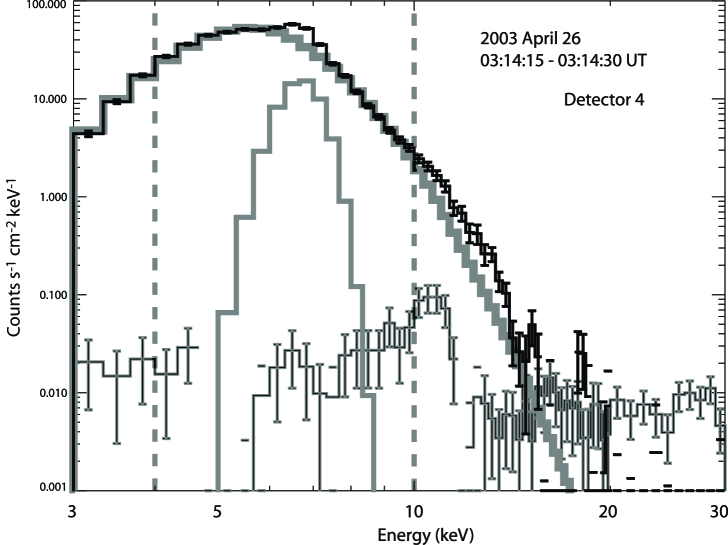
Figure 2: Upper panel: Count rate spectra (counts s^-1 cm^-2 keV^-1) in the energy range 3–30 keV from RHESSI detector 4 in the A0 attenuator state. The spectrum is during the flare on 2003 April 26 (03:14:15–03:14:30 UT). The histogram with thin dark line and error bars shows the observed count rate spectrum with uncertainties in each energy bin. The background spectrum is the histogram with error bars at a count rate level of $\sim 0.01$. The histograms with thick gray lines show the MEKAL continuum folded through the spectral response matrix and the Gaussian line feature representing the Fe-line (energy $\sim 6.7$ keV). The fit range was 4–10 keV (indicated by vertical dashed lines). The observed excess counts above the model spectrum $>10$ keV is the result of pulse pile-up and is not included in the fit. The reduced $\chi^{2}$ for the goodness of fit was 0.78. Lower panel: Residuals (i.e. numbers of standard deviations of the theoretical count rate above or below the measured rate) in the fit range.

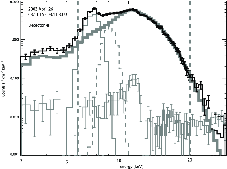
Figure 3: As for Fig. 2 but for RHESSI detector 4 in the A1 attenuator state during the 2003 April 26 flare (03:11:15–03:11:30 UT). Upper panel: The model spectrum includes the Fe line feature as well as a second line feature with peak energy $\sim 8$ keV (dashed gray histogram) representing the Fe/Ni line. The fit range indicated by vertical gray lines was 5.7–20 keV. The reduced $\chi^{2}$ was 0.78. Lower panel: Residuals of the fit in the fit range.

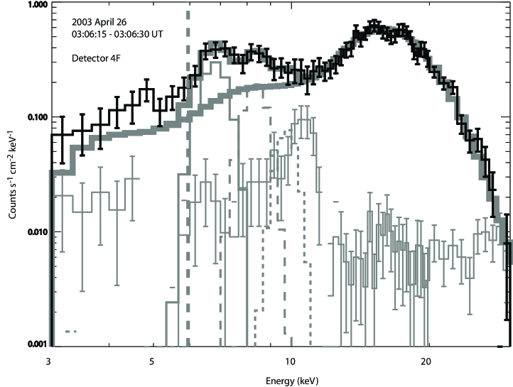
Figure 4: As for Fig. 2 but for RHESSI detector 4 in the A3 attenuator state during the 2003 April 26 flare (03:06:15–03:06:30 UT). Upper panel: The Fe and Fe/Ni line features are indicated as in Fig. 3. A third line feature has been added (gray histogram with short dashes) to account for an instrumentally formed line at $\sim 10$ keV. The fit range was 6–30 keV. The reduced $\chi^{2}$ was 0.69. Lower panel: Residuals of the fit in the fit range.

For the purposes of this analysis, assumed element abundances affect the continuum intensities (and therefore emission measure) because of the free–bound contribution to the continuum. As indicated above, we used a version of ospex that incorporates the mekal code with the solar coronal abundances of (Meyer, 1985). Use of coronal rather than photospheric abundances, for which the abundances of elements with first ionization potentials $<10$ eV are enhanced, is based on the fact that flare plasmas have been observed to have coronal abundances (Fludra & Schmelz, 1995; Phillips et al., 2003; Sylwester et al., 2006). The abundances of Meyer (1985) differ from the more recent values of Feldman & Laming (2000) by factors of up to 3, but the continuum intensity from the Meyer (1985) abundances is only 18% less than that from the Feldman & Laming (2000) abundances over the 7–12 keV range. If the Feldman & Laming (2000) abundances are more reliable, we may expect that the emission measures derived in this work are too large by 18%.

RHESSI photon spectra have been compared with those derived from the RESIK crystal spectrometer (Sylwester et al., 2005) on CORONAS-F, which operated between 2001 and 2003. This indicates that the RHESSI absolute fluxes at energies $\gtrsim 5$ keV are accurate to $\sim 20$%. RESIK is believed to be calibrated in absolute sensitivity to better than 20% in its first-order mode (energy range of 2.0–3.7 keV) with an energy resolution of $\lesssim 8$ eV or better. Although there is no overlap with the RHESSI energy range, the agreement of the extrapolated spectra is to within the estimated uncertainties of the flux calibration of both instruments for a period during the 2003 April 26 when RHESSI was in its A0 state (Dennis et al., 2005). This has been found for several other flares also, with RHESSI in A0. On the occasions when RESIK operated in its third diffraction order, the 6.7-keV Fe-line feature is included in one of its four channels; RESIK and RHESSI estimates of the total flux in this line feature during the 2003 April 26 flare agree to better than 50% (Dennis et al., 2005).

4 Results and Discussion

Table 1: Analyzed RHESSI flares

	Year	Date	Approx. GOES	GOES	Heliographic	Approx. UT range	RHESSI attenuator
			U.T. range	classa	coordinatesa	of analyzed	state(s) in the
			Start-Peak-End a			RHESSI data	analyzed UT range
1	2002	Mar. 10/11	10/22:21 - 10/23:25 - 11/00:29	M2.3	S08 E58	10/22:57 - 11/01:13	A1
2		Mar. 15/16	15/22:09 - 15/23:10 - 16/00:42	M2.2	S08 W03	15/23:33 - 16/00:30	A1
3		Apr. 14/15	14/23:34 - 15/00:14 - 15/00:25	M3.7	N19 W60	14/23:51 - 15/00:51	A1
4		Apr. 21	00:43 - 01:51 - 02:38	X1.7	S14 W84	02:09 - 06:20	A1 - A0
5		May. 07	08:46 - 08:52 - 08:55	C2.8	S20 W18	08:52 - 08:57	A0
6		May. 31	00:04 - 00:16 - 00:25	M2.4	N12 W48	00:08 - 00:30	A1
7		Jun. 01	03:50 - 03:57 - 04:01	M1.6	S19 E29	03:53 - 04:03	A1
8		Jul. 20/21	20/21:04 - 20/21:30 -20/21:54	X3.3	N17 E72	20/22:29 - 21/00:38	A1
9		Jul. 23	00:18 - 00:35 - 00:47	X4.8	S13 E72	01:00 - 02:30	A1
10		Jul. 26/27	26/22:36 - 26/22:38 - 26/22:41	M4.6	S19 E26	26/23:01 - 27/00:01	A1
11		Jul. 29	10:27 - 10:44 - 11:13	M4.7	S11 W15	10:50 - 11:26	A1
12		Aug. 24	00:49 - 01:12 - 01:31	X3.1	S02 W81	01:34 - 02:34	A1
13		Oct. 04	05:34 - 05:38 - 05:41	M4.0	S18 W08	05:41 - 05:48	A1
14		Dec. 02	19:19 - 19:27 - 19:33	C9.6	N09 E32	19:26 - 19:32	A1
15		Dec. 17	22:57 - 23:35 - 23:45	M1.6	S27 E01	23:20 - 23:52	A0 - A1
16	2003	Apr. 23	00:57 - 01:06 - 01:30	M5.2	N18 W16	01:02 - 01:17	A1
17		Apr. 26	03:01 - 03:06 - 03:12	M2.1	N19 W66	03:04 - 03:29	A3 - A1 - A0
18		May. 29	00:51 - 01:05 - 01:12	X1.1	S07 W31	00:45 - 01:21	A0 - A1
19		Aug. 14	22:28 - 22:44 - 23:15	C5.0	S17 W87	22:40 - 22:52	A1 - A0
20		Aug. 19	09:45 - 10:06 - 10:25	M2.7	S15 W68	09:59 - 10:45	A1
21		Oct. 22	19:47 - 20:07 - 20:28	M9.9	S17 E88	20:16 - 20:37	A1
22		Oct. 23	19:50 - 20:04 - 20:14	X1.1	S17 E88	19:59 - 20:31	A3 - A1
23		Nov. 02	17:03 - 17:25 - 17:39	X8.3	S18 W59	18:37 - 19:36	A1
24		Nov. 11	15:23 - 16:15 - 17:17	C8.5	S00 E90	16:00 - 18:10	A1 - A0
25	2004	Jan. 05	02:50 - 03:45 - 05:20	M6.9	S10 E36	04:06 - 04:52	A1
26		Jul. 20	12:22 - 12:32 - 12:45	M8.7	N10 E33	12:37 - 12:47	A3 - A1
27	2005	Jan. 15/16	15/22:25 - 15/23:02 - 15/23:31	X2.6	N14 W08	16/01:30 - 16/03:13	A1

Table 1 gives details of the 27 flares between 2002 and 2005 analyzed in this work. The GOES X-ray importance of these flares ranges from C2.8 to X8.3. The times of RHESSI spectral analysis and the attenuator states are given, as are the flare locations on the Sun.

Figure 5 shows the RHESSI count rates in three energy bands (background-subtracted), as well as the time histories of estimated values of emission measure, $T_{e}$, and the flux and equivalent width of the Fe-line feature during the M2 flare of 2002 May 31 (No. 6 in Table 1). Over this interval as well as the flare peak, RHESSI was in the A1 state. The photon counts in the 16–22 keV range indicate that there was no significant nonthermal component, a short impulsive phase having occurred at about 23:57 U.T. on May 30. A fit to 68 spectra over the range 5.3–16.7 keV in 20-s intervals shows close agreement between observed and model spectra having the mekal continua and two line features to match the Fe and Fe/Ni line features, with reduced $\chi^{2}$ steadily decreasing from approximately 1.2 at the earlier times to 0.8 at later times. An isothermal emitting plasma is a good approximation for all spectra, particularly those over the decline of this flare.

Figure 5: RHESSI 5-10 keV, 10-16 keV and 16-22 keV count rates (s^-1), emission measure (EM, units of $10^{49}$ cm^-3, logarithmic scale) and $T_{e}$ (MK), Fe-line feature flux (‘ph.’ = photons cm^-2 s^-1) and equivalent width (keV) for the M2 flare on 2002 May 31 (No. 6 in Table 1). The peak of the flare in GOES was at 00:16 U.T. The background spectrum in a 40-s night-time interval before the flare, at approximately 23:55 U.T., was subtracted from the measured count rate spectrum in each time interval during the flare. The uncertainties in these plots are indicated by the scatter of points about smooth curves through the points in each case.

The estimated equivalent widths of the Fe-line feature were plotted against $T_{e}$ for all intervals and compared with the theoretical values, taken from an updated version of that given by Phillips (2004). The theoretical curve has been revised as a result of changed definitions of the Fe line flux and the continuum flux at the line energy. In Phillips (2004), the line flux was taken to be the excess over the continuum after smoothing calculated spectra from the CHIANTI code to 1-keV resolution; this is here redefined to be the total of lines making up the Fe-line feature without smoothing. Also, in Phillips (2004), the line energy was taken to be the energy of the centroid of the line with continuum emission included, whereas a more satisfactory definition is the centroid energy of the line alone. As in Phillips (2004), Feldman & Laming’s (2000) coronal abundance of Fe (Fe/H $=1.26\times 10^{-4}$) is assumed, together with the ionization fractions of Mazzotta et al. (1998). The updated definition of the Fe line equivalent width leads to a maximum theoretical value of 4.0 keV at $T_{e}\sim 24$ MK, compared with 3.0 keV at $T_{e}\sim 23$ MK (Phillips, 2004). Figure 6 is a plot of the Fe line equivalent width, including the updated theoretical curve and observed points for the 2002 May 31 flare, the time variations of which are shown in Fig. 5. The observed equivalent widths were estimated from spectra in the A1 attenuator state over the period from shortly before the flare maximum to about 10 minutes after. From Fig. 6, it can be seen that the observed points follow a dependence with temperature that approximates the theoretical curve. The points on the flare decay are nearer to the curve than those on the flare rise or at the flare peak. Most points are generally lower than and to the right of the curve.

Figure 6: Measured Fe line equivalent widths (keV) plotted against $T_{e}$ (MK) during the flare of 2002 May 31 (No. 6 in Table 1). The solid curve is the theoretical dependence, revised from the calculations of Phillips (2004). Points in the A1 state during the rise phase (00:08–00:11 U.T.) of this flare are shown as diamonds; those at the peak (00:11–00:16 U.T.) as squares; those in the decay (00:16–00:30 U.T.) as black circles. The general sequence in time is indicated by arrows.

Plots for other flares similar to Fig. 6 show that the equivalent width increases with $T_{e}$ in ways that have varying degrees of agreement with the theoretical curve. Figure 7 shows Fe line equivalent width plots against $T_{e}$ for each of the 27 flares of this analysis. The theoretical curve identical to that in Fig. 6 is shown for each flare. As indicated in Table 1, most estimates of Fe line flux and equivalent width were made when RHESSI was in its A1 state since it was then that the best $\chi^{2}$ values were achieved. Estimates in other attenuator states are indicated in Fig. 7 by different symbols (see figure caption).

Patterns of the observed equivalent width variations can be discerned for most flares. These are most obvious for the 20 flares (nos. 1, 3, 4, 5, 6, 7, 10, 12, 13, 14, 15, 16, 17, 18, 19, 20, 21, 22, 25, and 26) for which there is a sequence of measurements covering a relatively large temperature range ($\gtrsim 5$ MK), often well into the flare decay. Most or all of the equivalent width estimates for each flare were made in the A1 attenuator state with the exceptions of flare 5, made in the A0 attenuator state, and flares 19, 22, and 26, partly made in the A3 attenuator state. For four flares (1, 3, 12, and 17), the observed equivalent widths lie below the theoretical curve, with clear evidence in at least the case of flare 3 that the observed equivalent widths saturate at high temperatures ($T_{e}\gtrsim 20-25$ MK). The observed maximum equivalent width in these four flares is approximately 80–90% of the theoretical maximum equivalent width (4.0 keV), with the observed equivalent widths at lower temperatures less than 80% of the theoretical value. For flare 5 (GOES class C2.8), the equivalent widths are only 40% of the theoretical values, although the A0 spectra at higher temperatures are fitted poorly by the model spectra and may be unreliable. For flare 7, the observed points cluster around the theoretical curve, while those for flare 20 are below the theoretical curve for $T_{e}\lesssim 18$ MK and agree with it for $T_{e}\gtrsim 18$ MK.

The equivalent widths of at least 15 flares (2, 4, 6, 8, 10, 13, 14, 15, 16, 18, 21, 22, 25, 26, and 27) rise with $T_{e}$, crossing the theoretical curve at temperatures from 15 MK to 28 MK. For flares 22 and 26, there is some evidence that without the A3 points the maximum equivalent width would be only slightly greater than 4 keV. In view of the often poor fits to model spectra with RHESSI in its A3 state, the presence of some A3 data may be misleading. For each of these 15 flares, the observed points rise with $T_{e}$ following a path that is clearly to the right of the theoretical curve.

Figure 7: Fe-line feature equivalent widths (keV, vertical axis) plotted against $T_{e}$ (MK, horizontal axis) estimated from RHESSI spectra during the 27 flares listed in Table 1. The curve is the theoretical equivalent width vs. $T_{e}$ for a coronal abundance of Fe (Fe/H $=1.26\times 10^{-4}$) and ionization fractions of Mazzotta et al. (1998). In this figure, estimated equivalent widths are distinguished according to the RHESSI attenuator state: squares (A0), circles (A1), and triangles (A3).

Fig. 7. — Continued.

Fig. 7. — Continued.

5 Summary and Conclusions

For this analysis of RHESSI solar flare data, low-energy ($\gtrsim 5$ keV) spectra during flares were fitted with model thermal spectra consisting of a continuum (free–free plus free–bound emission) from the mekal spectral code and line features with Gaussian profiles at 6.7 keV (the Fe line), $\sim 8$ keV (the Fe/Ni line), plus an instrumentally formed line at $\sim 10$ keV. The data analysis was performed with software that accounts for all known instrumental effects and allows for background subtraction. An isothermal approximation was used, so that the continuum slope and flux measure the temperature $T_{e}$ and emission measure $\int_{V}N_{e}^{2}dV$. The fits to the model spectra are most reliable (as measured by the reduced $\chi^{2}$) for RHESSI spectra taken in its A1 attenuator state during the decay of flares. Some 27 flares were selected from the RHESSI data set, chosen for their relatively long durations so that repeated measurements of the Fe line equivalent could be made, particularly during their decay stages. Measurements of the Fe line equivalent width were made from these fits to the observed spectra, and plots made for each flare of the equivalent width against $T_{e}$. Comparison was made with an updated version of the theoretical curve from Phillips (2004), which assumes the coronal abundance of Fe (Fe/H $=1.26\times 10^{-4}$, i.e. $4\times$ photospheric) derived by Feldman & Laming (2000). For only one flare (no. 7) is there good agreement between theory and observation, and near-agreement for another flare (no. 20). For four other flares (1, 3, 12, 17), the observed equivalent widths lie below the theoretical curve, the observed values reaching a maximum which is 80% of the theoretical value, $\sim 4$ keV. Agreement between the observations and theory for these four flares could be achieved if the coronal relative abundance of Fe were multiplied by 0.8 (i.e. Fe/H $\sim 1\times 10^{-4}$ or $3.2\times$ photospheric).

A more common characteristic is for the observed equivalent widths to rise with $T_{e}$, exceeding the theoretical curve at $T_{e}=15-28$ MK. With A3 spectral results included, the equivalent width for a few flares rises to a value of $\sim 8$ keV, more than double the maximum of the theoretical curve. If the A3 points are disregarded, the observed points rise to a value of slightly more than 4 keV. The observed equivalent widths increase with $T_{e}$ more sharply than is predicted by the theoretical curve, with a clear displacement to higher temperatures being indicated. These results are not so easily explained. If the isothermal approximation is a good one for spectra during these flares, as is indicated by the reduced $\chi^{2}$ values, then possibly this behavior could indicate the need for a correction to the ionization fractions of Mazzotta et al. (1998). In particular, the displacement indicates that the value of $N({\rm Fe}^{+24})/N({\rm Fe})$ ($N({\rm Fe}^{+24})=$ the number density of He-like Fe and $N({\rm Fe})=$ the number density of all Fe ions) should be lower than is calculated for the temperature range $12<T_{e}\,({\rm MK})<18$.

Antonucci et al. (1987) suggested corrections to the $N({\rm Fe}^{+23})/N({\rm Fe}^{+24})$ ratio based on Solar Maximum Mission crystal spectrometer data. This ratio is equal to $Q/R$ where $Q$ is the rate coefficient of ionizations from Fe⁺²³ and $R$ the rate coefficient of recombinations to Fe⁺²⁴, both functions of $T_{e}$. Antonucci et al. (1987) argued that, since the various theoretical rate coefficients of ionization from the Fe⁺²³ available then had more scatter than the rate coefficients of recombinations to Fe⁺²⁴, and that the recombination rates were more slowly varying with $T_{e}$ than the ionization rates, the ionization rates were more likely to require revision than the recombination rates. The ionization rate coefficients in the work of Mazzotta et al. (1998) are based on analytical formulae that are known to be a good representation of measured data for ions up to Fe⁺¹⁵ (Arnaud & Raymond, 1992). However, there is a need for the inclusion of ionization fractions based on experimental data for ionization rates from Fe⁺²³ and other ions, now available (e.g. Wong et al. (1993)). Our result is consistent with the number density of Fe⁺²⁴ ions being too small compared with that of lower stages like Fe⁺²³, but it is difficult to explain why the temperature displacement varies from flare to flare, as found here. Possibly non-equilibrium effects play a role, but this is unlikely in view of the probable high densities ($N_{e}\sim 10^{11}$ cm^-3) of the emitting plasma, as was shown by Phillips (2004).

The tendency of Fe-line feature equivalent widths to agree better with theory for periods when flares are in their declining stage and RHESSI is in its A1 attenuator state is probably due to the flares having a more nearly isothermal state in their decay. This has also been found from temperature measurements using Ca XIX and S XV line ratios using the Bragg Crystal Spectrometer on the Yohkoh spacecraft (Phillips et al., 2005b). Flares probably depart most strongly from an isothermal state in their early and peak stages, when images (particularly those from RHESSI and the TRACE 195 Å filter: Gallagher et al. (2002), Phillips et al. (2005a)) show emission in loop-top structures at high temperatures in close proximity with loop structures with much lower temperatures. The general lack of agreement of Fe line feature equivalent widths observed late in flare developments by RHESSI in the A0 state is therefore unexpected on this basis, but this appears to be due, at least occasionally, to the degraded spectral resolution at high count rates and the difficulty of distinguishing the line feature at low count rates and at low temperatures.

Multi-thermal flare plasmas are being investigated and will be the subject of a further analysis of RHESSI flare spectra. Differential emission measures, DEM $=N_{e}^{2}dV/dT_{e}$, can be extracted from spectral line fluxes and other data. Procedures like the PintofAle code (Kashyap & Drake, 2000) and DEMON (Sylwester et al., 1980) are currently being compared, using spectral data from RHESSI, the CORONAS-F RESIK crystal spectrometer, GOES, and other broad-band data. Simpler procedures using analytical forms for DEM are also being tried, such as DEM $=$ exp$(-T_{e}/T_{0})$ ($T_{0}$ is a constant for a particular time), since RESIK data for Si XII dielectronic satellite line intensity ratios show that such a function is an improvement over an isothermal approximation (Phillips et al., 2006).

K.J.H.P. acknowledges support from a National Research Council Senior Research Associateship award. C.C.’s work was supported by a Research Assistantship from the Catholic University of America and NASA/GSFC. We are grateful to M. Berg, D. W. Savin, R. A. Schwartz, and A. K. Tolbert for their help.

References

- Antonucci et al. (1987) Antonucci, E., Dodero, M. A., Gabriel, A. H., Tanaka, K., & Dubau, J. 1987, A&A, 180, 263
- Arnaud & Raymond (1992) Arnaud, M., & Raymond, J. 2005, ApJ, 398, 394
- Caspi et al. (2006) Caspi, A., et al. 2006, in preparation
- Dennis et al. (2004) Dennis, B. R., Hudson, H. S., & Krucker, S. 2004, Proc. CESRA Workshop, Isle of Skye, Scotland
- Dennis et al. (2005) Dennis, B. R., Phillips, K. J. H., Sylwester, J., Sylwester, B., Schwartz, R. A., Tolbert, A. K. 2005, Adv. Space Res., 35, 1723
- Feldman & Laming (2000) Feldman, U., & Laming, M. 2000, Phys. Scripta, 61, 222
- Fludra & Schmelz (1995) Fludra, A., & Schmelz, J. T. 1995, ApJ, 447, 936
- Gallagher et al. (2002) Gallagher, P. T., Dennis, B. R., Krucker, S., Schwartz, R. A., & Tolbert, A. K. 2002, Sol. Phys., 210, 341
- Hurford et al. (2002) Hurford, G. J., et al. 2002, Sol. Phys., 210, 61
- Kashyap & Drake (2000) Kashyap, V. & Drake, J. J. 2000, BASI, 28, 475
- Landi et al. (2005) Landi, E., et al. 2006, ApJS, 162, 261
- Lin et al. (2002) Lin, R. P., et al. 2002, Sol. Phys., 210, 3
- Mazzotta et al. (1998) Mazzotta, P., Mazzitelli, G., Colafrancesco, S., & Vittorio, N. 1998, A&AS, 133, 403
- Mewe et al. (1985) Mewe, R., Lemen, J. R., Peres, G., Schrijver, J., & Serio, S. 1985, A&A, 152, 229
- Meyer (1985) Meyer, J.-P 1985, ApJS, 57, 173
- Neupert et al. (1969) Neupert, W. M., White, W. A., Gates, W. J., Swartz, M., & Young, R. M. 1969, Sol. Phys., 6, 183
- Phillips et al. (2003) Phillips, K. J. H., Sylwester, J., Sylwester, B., & Landi, E. 2003, ApJ, 589, L113
- Phillips (2004) Phillips, K. J. H. 2004, ApJ, 605, 921
- Phillips et al. (2005a) Phillips, K. J. H., Chifor, C., & Landi, E. 2005a, ApJ, 626, 1110
- Phillips et al. (2005b) Phillips, K. J. H., Feldman, U., & Harra, L. K. 2005b, ApJ, 634, 641
- Phillips et al. (2006) Phillips, K. J. H., Dubau, J., Sylwester, J., & Sylwester, B. 2006, ApJ, 638, 1154
- Smith et al. (2002) Smith, D. M., et al. 2002, Sol. Phys., 210, 33
- Sylwester et al. (1980) Sylwester, J., Schrijver, J., & Mewe, R. 1980, Sol. Phys., 67, 285
- Sylwester et al. (2005) Sylwester, J., et al. 2005, Sol. Phys., 226, 45
- Sylwester et al. (2006) Sylwester, J., Sylwester, B., Phillips, K. J. H., Culhane, J. L., Brown, C., Lang, J., & Stepanov, A. I. 2006, Adv. Space Res., in press
- Wong et al. (1993) Wong, K. L., Beiersdorfer, P., Chen, M. H., Marrs, R. E., Reed, K. J., Scofield, J. H., Vogel, D. A., & Zasadzinski, R. 1993, Phys. Rev. A, 48(4), 2850