A New Measure for Weak Lensing Flexion

Abstract

We study a possibility to use the octopole moment of gravitationally lensed images as a direct measure of the third-order weak gravitational lensing effect, or the gravitational flexion. It turns out that there is a natural relation between flexion and certain combinations of octopole/higher-multipole moments which we call the Higher Order Lensing Image’s Characteristics (HOLICs). This will allow one to measure directly flexion from observable octopole and higher-multipole moments of background images. We show based on simulated observations how the use of HOLICs can improve the accuracy and resolution of a reconstructed mass map, in which we assume Gaussian uncertainties in the shape measurements estimated using deep $i^{\prime}$-band data of blank fields observed with Suprime-Cam on the Subaru telescope.

1 Introduction

It is now widely recognized that weak gravitational lensing is a unique and valuable tool to study the mass distribution of clusters of galaxies as well as large scale structure in the universe since it directly measures the projected mass distribution of the lens regardless of the physical state of the system and the nature of matter content (Bartelmann & Schneider 2001). In the usual treatment of the weak lensing analysis, the quadrupole moment of background galaxy images is used to quantify the image ellipticity. Then the lensing properties are extracted from the image ellipticities by assuming that source galaxies are randomly oriented in the absence of gravitational lensing. In practice we average over a local ensemble of image ellipticities to estimate the lensing properties. The local ensemble should contain a sufficient number of background galaxies to increase the signal-to-noise ratio of local shear measurements, whereas the region that contains the galaxies should be small enough to guarantee the constancy of the lensing properties over the region. The latter condition is necessary in the usual prescription for weak lensing because it is based on the locally linearized lens equation. On the other hand, the former limits the resolution of mass maps reconstructed via weak lensing techniques, which is of the order 1 arcmin in ground-based observations.

Space-based high-resolution imaging surveys, such as the Cosmic Evolution Survey (Scoville et al. 2007) with the Hubble Space Telescope (HST) and the proposed Supernova/Acceleration Probe (SNAP) wide weak lensing survey (Massey et al. 2004), will provide significant gains with a higher surface number density of well-resolved galaxies due to the small, stable Point Spread Function (PSF), which will enable high-resolution mapping of the lensing mass distribution down to an angular resolution of $\sim 0\farcm 1$. On the other hand, such a small PSF will allow us to resolve not only the elliptical component, described by the quadrupole moment, but also higher-order shape properties of background galaxy images, which could also carry some sort of information of lensing properties. It may be therefore interesting to see if such higher multipole moments of the shape are useful for the weak lensing analysis.

There have been some attempts to generalize the weak lensing analysis to include higher order moments of the light distribution. Goldberg and Natarajan (2002) suggested that higher order effects in gravitational lensing, described by the third order derivatives of the lensing potential, can give rise to octopole moments of the light distribution for background galaxies. Goldberg and Bacon (2005) have further developed their approach and proposed a new inversion technique based on the Shapelets formalism (Refregier 2003; Refreger & Bacon 2003; Massey and Refregier 2005), and labeled this third order effect as the flexion of background images. Irwin and Shmokova (2006) developed a similar analysis method for measuring the higher order lensing effects and applied this method to the HST Deep Field North. Recently Irwin, Shmokova, & Anderson 2006 reported on the detection of lensing signals in the UDF due to small scale structure using their ”cardioid” and ”displacement” techniques. Recently Goldberg & Leonard (2006) has extended our HOLICs approach to developed a method to correct HOLICs for the effect of isotropic Point Spread Function (PSF).

In the present paper, following the flexion formalism by Bacon et al. (2006), we study a possibility to use higher multipole moments of background source images for the weak lensing analysis, and demonstrate via simulations how such higher order moments can improve the accuracy and resolution of a weak lensing mass reconstruction.

The paper is organized as follows. After briefly summarizing the basis of weak lensing and the flexion formalism in section 2, we introduce higher multipole moments of galaxy images in section 3. We define certain combinations of higher multipole moments as HOLICs (Higher Order Lensing Image’s Characteristics) and establish an explicit relation between flexion and HOLICs. In section 4 we present simulations of a weak lensing mass reconstruction using mock observational data of image ellipticities and HOLICs. Finally some discussions and comments are given in section 5.

2 Basis of Weak Lensing and Flexion

In this section we briefly summarize general aspects of weak lensing and Bacon et al.’s flexion formalism. A general review of weak lensing can be found in Bartelmann & Schneider (2001), and we follow the notations and conventions therein.

2.1 Local Lens Mapping

The gravitational deflection of light ray can be described by the lens equation,

$$\mbox{\boldmath$\beta$}=\mbox{\boldmath$\theta$}-\mbox{\boldmath$\nabla$}\psi(\mbox{\boldmath$\theta$}),$$ (1)

where $\psi(\mbox{\boldmath$\theta$})$ is the effective lensing potential; $\psi$ is defined via the 2D Poisson equation as $\nabla^{2}\psi(\mbox{\boldmath$\theta$})=2\kappa(\mbox{\boldmath$\theta$})$, with the lensing convergence $\kappa$. The convergence $\kappa=\Sigma_{m}/\Sigma_{\rm crit}$ is the dimensionless surface mass density projected on the sky, which depends on the lens redshift $z_{d}$ and the source redshift $z_{s}$ as well as the background cosmology through the critical surface mass density

$$\Sigma_{\rm crit}=\frac{c^{2}}{4\pi G}\frac{D_{s}}{D_{d}D_{ds}},$$ (2)

where $D_{d}$, $D_{s}$, and $D_{ds}$ are the angular-diameter distances from the observer to the deflector, from the observer to the source, and from the deflector to the source, respectively. If the angular size of an image is small enough to be able to neglect the change of the lensing potential $\psi(\mbox{\boldmath$\theta$})$, then we can linearize locally the lens equation (1) to have $\delta\beta_{i}={\cal A}_{ij}(\mbox{\boldmath$\theta$})\delta\theta_{j}$, where ${\cal A}_{ij}$ is the Jacobian matrix of the lens equation,

$${\cal A}_{ij}\equiv\left(\frac{\partial\mbox{\boldmath$\beta$}}{\partial\mbox{\boldmath$\theta$}}\right)_{ij}=\delta_{ij}-\psi_{,ij}\equiv(1-\kappa)\delta_{ij}-\gamma_{ij}$$ (3)

where $\gamma_{ij}$ is the trace-free, symmetric shear matrix,

$$\gamma_{ij}:=\left(\frac{\partial^{2}}{\partial^{i}\partial^{j}}-\frac{1}{2}\nabla^{2}\delta_{ij}\right)\psi=\left(\begin{array}[]{cc}\gamma_{1}&\gamma_{2}\\ \gamma_{2}&-\gamma_{1}\end{array}\right)$$ (4)

being defined with the components of gravitational shear $\gamma=\gamma_{1}+i\gamma_{2}$.

2.2 Gravitational Shear and Quadrupole Shape Moments

In the usual treatment of weak lensing analysis, we use quadrupole moments $Q_{ij}$ of the surface brightness distribution $I(\mbox{\boldmath$\theta$})$ of background images for quantifying the shape of the images:

$$Q_{ij}\equiv\frac{\int\!d^{2}\theta\,q_{I}[I(\mbox{\boldmath$\theta$})]\Delta\theta_{i}\Delta\theta_{j}}{\int d^{2}\theta\,q_{I}[I(\mbox{\boldmath$\theta$})]}$$ (5)

where $q_{I}[I(\mbox{\boldmath$\theta$})]$ denotes the weight function used in the shape measurement, and $\Delta\theta_{i}=\theta_{i}-\bar{\theta_{i}}$ is the offset vector from the image centroid. Then we define the complex ellipticity $\chi$ as

$$\chi\equiv\frac{Q_{11}-Q_{22}+2iQ_{12}}{Q_{11}+Q_{22}}.$$ (6)

The complex ellipticity $\chi$ transforms under the lens mapping as

$$\chi^{(s)}=\frac{\chi-2g+g^{2}\chi^{\ast}}{1+|g|^{2}-2Re(g\chi^{\ast})}$$ (7)

where $g=\gamma/(1-\kappa)$ is the reduced shear and ^∗ denotes complex conjugate. In the weak lensing limit, we neglect 2nd order terms of $g$ and $\chi$, which yields $\chi^{(s)}\approx\chi-2\gamma$. Assuming the random orientation of the source images, we average observed ellipticities over a sufficient number of images to obtain

$$\langle\chi\rangle\approx 2g\approx 2\gamma.$$ (8)

The inversion equation from the shear map to the convergence map is obtained in Fourier space as (Kaiser & Squires 1993)

$$\hat{\kappa}_{\gamma}(\mbox{\boldmath$k$})=\frac{k_{1}^{2}-k_{2}^{2}-2ik_{1}k_{2}}{k_{1}^{2}+k_{2}^{2}}\hat{\gamma}(\mbox{\boldmath$k$})\ \ \ \ (\mbox{\boldmath$k$}\neq 0).$$ (9)

2.3 Spin Properties

We define the spin for weak lensing quantities. A quantity is said to have spin-$N$ if it has the same value after rotation by $2\pi/N$. Then, the complex shear $\gamma$, the reduced shear $g$, and the complex ellipticity $\chi$ are all spin-2 quantities. The product of spin-$A$ and spin-$B$ quantities has spin-$(A+B)$, and the product of spin-$A$ and spin-$B^{*}$ has spin-$(A-B)$.

2.4 Flexion

Flexion is introduced to be the third-order lensing effect responsible for the weakly skewed and arc-like appearance of lensed galaxies. The third-order lensing effect arises from the fact that the shear and the convergence are not constant within a source galaxy image. By taking higher order derivatives of the lensing potential $\psi(\mbox{\boldmath$\theta$})$, we can deal with higher order transformations of the shape quantities than the complex ellipticity.

Flexion consists of four components of the third-order lensing tensor ${\cal D}_{ijk}={\cal A}_{ij,k}=-\psi_{,ijk}$ (see Bacon, Goldberg, Rowe, Taylor 2005). The first flexion ${\cal F}$ is defined as

$${\cal F}={\cal F}_{1}+i{\cal F}_{2}\equiv\partial\partial\partial^{*}\psi=|{\cal F}|e^{i\phi}=\partial\kappa,$$ (10)

and the second flexion ${\cal G}$ is defined as

$${\cal G}={\cal G}_{1}+i{\cal G}_{2}\equiv\partial\partial\partial\psi=|{\cal G}|e^{3i\phi}=\partial\gamma,$$ (11)

where $\partial=\partial_{1}+i\partial_{2}$ is the complex gradient operator, which transforms under rotation as a vector, $\partial^{\prime}=\partial e^{\phi}$, where $\phi$ is the angle of rotation. Thus ${\cal F}$ has spin-$1$ and ${\cal G}$ has spin-$3$. The two complex flexion fields satisfy the following consistency relation:

$$\partial^{*}\partial{\cal G}=\partial\partial{\cal F}.$$ (12)

We then describe the transformation of the shape of a background source by expanding the lens equation (1) to the second order as

$$d\beta_{i}\approx{\cal A}_{ij}d\theta_{j}+\frac{1}{2}{\cal D}_{ijk}d\theta_{j}d\theta_{k}.$$ (13)

The third-order lensing tensor ${\cal D}_{ijk}$ can be expressed as the sum of the two terms, ${\cal D}_{ijk}={\cal F}_{ijk}+{\cal G}_{ijk}$, with the spin-1 part ${\cal F}_{ijk}$ and the spin-3 part ${\cal G}_{ijk}$:

$${\cal F}_{ij1}=-\frac{1}{2}\left(\begin{array}[]{@{\,}cc@{\,}}3{\cal F}_{1}&{\cal F}_{2}\\ {\cal F}_{2}&{\cal F}_{1}\end{array}\right) \ \ {\cal F}_{ij2}=-\frac{1}{2}\left(\begin{array}[]{@{\,}cc@{\,}}{\cal F}_{2}&{\cal F}_{1}\\ {\cal F}_{1}&3{\cal F}_{2}\end{array}\right),$$ , (18)

$${\cal G}_{ij1}=-\frac{1}{2}\left(\begin{array}[]{@{\,}cc@{\,}}{\cal G}_{1}&{\cal G}_{2}\\ {\cal G}_{2}&-{\cal G}_{1}\end{array}\right) \ \ {\cal G}_{ij2}=-\frac{1}{2}\left(\begin{array}[]{@{\,}cc@{\,}}{\cal G}_{2}&-{\cal G}_{1}\\ -{\cal G}_{1}&-{\cal G}_{2}\end{array}\right).$$ , (23)

Flexion has a dimension of length^-1 (or angle^-1). This means that the effect by flexion depends on the source size. The shape quantities affected by the first flexion ${\cal F}$ alone have spin-$1$ properties, while those affected by the second flexion ${\cal G}$ alone have spin-$3$ properties.

From equations (10) and (11), the inversion equations from flexion to the convergence can be obtained as follows (Bacon et al. 2006):

$$(\kappa+iB)_{\cal F} = \triangle^{-1}\partial^{*}{\cal F},$$ (24)

$$(\kappa+iB)_{\cal G} = \triangle^{-2}\partial^{*}\partial^{*}\partial^{*}{\cal G},$$ (25)

where the complex part $iB$ describes the $B$-mode component that can be used to test the noise properties of weak lensing data. An explicit representation for the inversion equations is obtained in Fourier space as follows:

$$\hat{\kappa}_{\cal F}(\mbox{\boldmath$k$}) = -i\frac{k_{1}\hat{\cal F}_{1}+k_{2}\hat{\cal F}_{2}}{k_{1}^{2}+k_{2}^{2}},$$ (26)

$$\hat{\kappa}_{\cal G}(\mbox{\boldmath$k$}) = -i\frac{\hat{\cal G}_{1}(k_{1}^{3}-3k_{1}k_{2}^{2})+\hat{\cal G}_{2}(3k_{1}^{2}k_{2}-k_{2}^{3})}{(k_{1}^{2}+k_{2}^{2})^{2}},$$ (27)

for $\mbox{\boldmath$k$}\neq 0$. Further we can combine independent mass reconstructions $\hat{\kappa}_{a}(\mbox{\boldmath$k$})$ $(a=\gamma,{\cal F},{\cal G})$ linearly in Fourier space to improve the statistical significance of the $\kappa$ map with minimum noise variance weighting:

$$\hat{\kappa}(\mbox{\boldmath$k$})=\frac{\sum_{a}\hat{W}_{\kappa a}(\mbox{\boldmath$k$})\hat{\kappa}_{a}(\mbox{\boldmath$k$})}{\sum_{a}\hat{W}_{\kappa a}(\mbox{\boldmath$k$})},$$ (28)

where $\hat{W}_{\kappa a}(\mbox{\boldmath$k$})=1/P^{(N)}_{\kappa a}(\mbox{\boldmath$k$})$ with noise power spectrum $P^{(N)}_{\kappa a}(\mbox{\boldmath$k$})$ of a $\kappa$ map reconstructed using $a$th observable:

$$P^{(N)}_{\kappa\gamma}(\mbox{\boldmath$k$}) = \frac{P_{\gamma}^{(N)}(\mbox{\boldmath$k$})}{2}=\frac{\sigma^{2}_{\gamma}}{8\pi n_{g}}$$

$$P^{(N)}_{\kappa F}(\mbox{\boldmath$k$}) = \frac{P^{(N)}_{F}(\mbox{\boldmath$k$})}{2k^{2}}=\frac{\sigma^{2}_{F}}{8\pi n_{g}\mbox{\boldmath$k$}^{2}}$$ (29)

$$P^{(N)}_{\kappa G}(\mbox{\boldmath$k$}) = \frac{P^{(N)}_{G}(\mbox{\boldmath$k$})}{2k^{2}}=\frac{\sigma^{2}_{G}}{8\pi n_{g}\mbox{\boldmath$k$}^{2}}$$

with $P^{(N)}_{a}(\mbox{\boldmath$k$})$ being the shot noise power of $a$th observable, $\sigma_{a}$ being the intrinsic dispersion of $a$th observable, and $n_{g}$ being the surface number density of background galaxies. Assuming that errors in $\hat{\kappa}_{a}(\mbox{\boldmath$k$})$ between different observables are independent, the noise power spectrum for the estimator (28) is obtained as

$$P^{(N)}_{\kappa}(\mbox{\boldmath$k$})=\frac{1}{\sum_{a}\hat{W}_{a}(\mbox{\boldmath$k$})}=\frac{1}{\sum_{a}1/P^{(N)}_{\kappa a}(\mbox{\boldmath$k$})}.$$ (30)

3 Higher multipole moments of images: HOLICs

In this section we consider higher multipole moments of images and define useful combinations of them as Higher Order Lensing Image’s Characteristics (HOLICs). We then derive a simple, explicit relation between flexion and HOLICs.

Higher order moments of images are defined as a straightforward extension of the quadrupole moment. The octopole moment $Q_{ijk}$ and the 16-pole moment $Q_{ijkl}$ are define as follows:

$$Q_{ijk}\equiv\frac{\int\!d^{2}\theta\,q_{I}[I(\mbox{\boldmath$\theta$})]\Delta\theta_{i}\Delta\theta_{j}\Delta\theta_{k}}{\int\!d^{2}\theta\,q_{I}[I(\mbox{\boldmath$\theta$})]},$$ (31)

$$Q_{ijkl}\equiv\frac{\int\!d^{2}\theta\,q_{I}[I(\mbox{\boldmath$\theta$})]\Delta\theta_{i}\Delta\theta_{j}\Delta\theta_{k}\Delta\theta_{l}}{\int\!d^{2}\theta\,q_{I}[I(\mbox{\boldmath$\theta$})]}.$$ (32)

We first define the normalization factor $\xi$ as

$$\xi\equiv Q_{1111}+2Q_{1122}+Q_{2222}$$ (33)

with spin-0. Then, we define the following combinations of octopole moments as our HOLICs:

$$\zeta \equiv \frac{(Q_{111}+Q_{122})+i(Q_{112}+Q_{222})}{\xi},$$ (34)

$$\delta \equiv \frac{(Q_{111}-3Q_{122})+i(3Q_{112}-Q_{222})}{\xi},$$ (35)

where the first HOLICs $\zeta$ has spin-1, and the second HOLICs $\delta$ has spin-3. Note that HOLICs have the dimension of [length]^-1 (or angle^-1), the same as flexion does.

Now we are in a position to derive the transformation law of HOLICs under gravitational lensing. For this purpose we first derive the relation between the source octopole moment $Q^{(s)}_{ijk}$ and the image octopole moment $Q_{ijk}$. A straightforward calculation leads to

$$Q_{ijk}^{(s)} \approx {\cal A}_{il}{\cal A}_{jm}{\cal A}_{kn}Q_{lmn}+\frac{1}{2}\bigl{(}{\cal A}_{il}{\cal A}_{jm}{\cal D}_{kno}+{\cal A}_{jm}{\cal A}_{kn}{\cal D}_{ilo}$$ (36)

$$+{\cal A}_{il}{\cal A}_{kn}{\cal D}_{jmo}-4{\cal A}_{il}{\cal A}_{jm}{\cal A}_{kn}F_{o}\bigr{)}Q_{lmno}$$

where we have used the fact that the integration measures in the source and image planes are related in the following way (see Appendix A for detailed calculations):

$$d^{2}\beta = \left|\frac{\partial\mbox{\boldmath$\beta$}}{\partial\mbox{\boldmath$\theta$}}\right|d^{2}\theta$$ (37)

$$= (1-\kappa)^{2}(1-2F_{1}\Delta\theta_{1}-2F_{2}\Delta\theta_{2})\,d^{2}\theta,$$

to the first order of reduced flexion defined as

$$F := F_{1}+iF_{2}=\frac{\cal F}{1-\kappa}$$ (38)

$$G := G_{1}+iG_{2}=\frac{\cal G}{1-\kappa}.$$ (39)

Note that the flexion term from the determinant does not yield a net contribution to the denominators of equations (31) and (32) since the coordinate system is taken such that the first moment of $I(\mbox{\boldmath$\theta$})$ vanishes:

$$\int\!d^{2}\beta\,q_{I}[I(\mbox{\boldmath$\theta$})]\approx(1-\kappa)^{2}\int\!d^{2}\theta q_{I}[I(\mbox{\boldmath$\theta$})],$$ (40)

where we have neglected the second order term in $\gamma$. From this transformation law one obtains the desired expressions as

$$\zeta^{(s)} = \frac{\zeta-2g\zeta^{*}-g^{*}\delta-\frac{1}{4}(8F^{*}\eta+9F+2G\eta^{*}+G^{*}\lambda)}{(1-\kappa)(1-4Re[g^{*}\lambda]-5Re[F\iota_{I}^{*}]-Re[G\iota_{III}^{*}])},$$ (41)

$$\delta^{(s)} = \frac{\delta-3g\zeta-\frac{1}{4}(10F\eta+7F^{*}\lambda+3G)}{(1-\kappa)(1-4Re[g^{*}\lambda]-5Re[F\iota_{I}^{*}]-Re[G\iota_{III}^{*}])},$$ (42)

where dimensionless quantities $\eta$ and $\lambda$ are defined with 16-pole moments by

$$\eta \equiv \frac{(Q_{1111}-Q_{2222})+2i(Q_{1112}+Q_{1222})}{\xi},$$ (43)

$$\lambda \equiv \frac{(Q_{1111}-6Q_{1122}+Q_{2222})+4i(Q_{1112}-Q_{1222})}{\xi},$$ (44)

with spin-2 and spin-4, respectively; $\iota_{I}$, $\iota_{III}$ and $\iota_{V}$ are defined with $32$-pole moments by

$$\iota_{I} \equiv \frac{(Q_{11111}+2Q_{11122}+Q_{12222})+i(Q_{11112}+2Q_{11222}+Q_{22222})}{\xi},$$

$$\iota_{III} \equiv \frac{(Q_{11111}-2Q_{11122}-3Q_{12222})+i(3Q_{11112}+2Q_{11222}-Q_{22222})}{\xi},$$

$$\iota_{V} \equiv \frac{(Q_{11111}-10Q_{11122}+5Q_{12222})+i(5Q_{11112}-10Q_{11222}+Q_{22222})}{\xi},$$

with spin-1, spin-3, and spin-5, respectively.

Assuming that the quantities $g,\eta$ and $\lambda$ are small and neglecting higher-order terms containing $32$-pole moments which are reasonable assumptions on the weak lensing data, we can approximate the above equations as

$$\zeta^{(s)} \approx \zeta-\frac{9}{4}\frac{\cal F}{1-\kappa},$$ (46)

$$\delta^{(s)} \approx \delta-\frac{3}{4}\frac{\cal G}{1-\kappa}.$$ (47)

The formulae (46) make it possible to relate directly the flexion fields and the HOLICs measurements. Since the $\zeta$ and $\delta$ are quantities with non-zero spin, namely quantities with directional dependence, the expectation values of intrinsic $\zeta$ and $\delta$ are assumed to vanish,

$$\langle\zeta\rangle \approx \frac{9}{4}\frac{\cal F}{1-\kappa}\approx\frac{9}{4}{\cal F},$$ (48)

$$\langle\delta\rangle \approx \frac{3}{4}\frac{\cal G}{1-\kappa}\approx\frac{3}{4}{\cal G}.$$ (49)

Neglecting the flexion term in the Jacobian matrix (37) will lead to a reduction of the response $\langle\zeta\rangle/{\cal F}$ from $9/4$ to $5/4$ while it will keep the response $\langle\delta\rangle/{\cal G}$ unchanged, which was found earlier by Irwin & Shmakova 2006. In this way, one can measure directly the flexion fields ${\cal F}(\mbox{\boldmath$\theta$})$ and ${\cal G}(\mbox{\boldmath$\theta$})$ from the observable HOLICs. Once we obtain the flexion fields, we can make use of equations (26) and (27) to invert them to the surface mass distribution.

It is important to note the above relation (48) is modified if we take into account the fact that the ”apparent” center of an image defined by the first moment of the image is different from the ”actual” center mapped by the lens equation from the center of the source. We discuss in detail this shift of the centroid in Appendix B.

4 Simulated Observations

In order to test the performance of mass reconstructions based on HOLICs measurements, we generate simulated observations of the weak lensing effects, namely $(\chi,\zeta,\delta)$, that include observational errors as Gaussian uncertainties. The flexion fields (${\cal F}(\mbox{\boldmath$\theta$})$, ${\cal G}(\mbox{\boldmath$\theta$}$)) can be used to reconstruct mass maps directly, independent of information on the shear field $\gamma(\mbox{\boldmath$\theta$})$ (see §2.4). The equation (46) defines the direct, unbiased estimators for the flexion fields, where the precision of this measurement depends on the intrinsic values of HOLICs convolved with the measurement noise. In the present simulation we do not take into account explicitly the centroid shift (see Appendix B) but use directly equations (41) and (42) to calculate the lensed HOLICs from the intrinsic shape quantities and lens properties, which does not require the measurement and removal of the apparent centroid of an image.

To determine the widths of random Gaussian distributions for the noise component of HOLICs $(\zeta,\delta)$, arising from the intrinsic scatter in unlensed HOLICs and observational noise, we refer to variances of HOLICs obtained from our preliminary study of deep $i^{\prime}$-band data of $\sim 2\times 4$ ${\rm deg}^{2}$ blank fields observed with Suprime-Cam on the Subaru telescope (T. Yamada, private communication). Each $4{\rm deg}^{2}$ data set consists of $18$ Suprime-Cam pointings with $0\farcs 202$ pixel^-1. We used our weak lensing analysis pipeline based on IMCAT (Kaiser, Squires, & Broadhurst 1995) extended to include the higher multipole moments in the shape measurements. We selected a sample of $493934$ background galaxies with $20\leq i^{\prime}_{\rm AB}\leq 24.5$ mag in the blank fields, corresponding to a mean surface number density of $\bar{n}_{g}\approx 17\,{\rm arcmin}^{-2}$. Here we discarded stars and all objects for which reliable shape measurements cannot be found. In particular, we excluded those small objects whose half-light radius $(r_{h})$ is smaller than $0\farcs 50$ (2.5 pixels). We note the median value of stellar $r_{h}$ over the entire field is $\langle r_{h}^{*}\rangle_{\rm med}\approx 0\farcs 40$ with a dispersion of $0\farcs 08$ using $N_{*}=27958$ stars ($n_{*}\approx 1\,{\rm arcmin}^{-2}$). This lower cut-off in the galaxy size is essential for us to be able to make reliable shape measurements because (1) the smaller the object, the noisier its shape measurement due to pixelization (i.e. discretization) noise, in particular for the case of higher-order shape moments, and (2) the shape of an image whose intrinsic size is smaller than or comparable to the size of PSF can be highly distorted and smeared. For example, if the spatial distributions of both the source and the PSF are described by a two-dimensional Gaussian, with half-light radii of $r_{h,0}$ and $r_{h}^{*}$, respectively, then the half-light radius of the PSF-convolved image is $r_{h}=\sqrt{r_{h,0}^{2}+r_{h}^{*2}}$. When both the sizes are equal, then $r_{h}=\sqrt{2}r_{h}^{*}$, which is close to our choice for the lower cut-off in $r_{h}$.

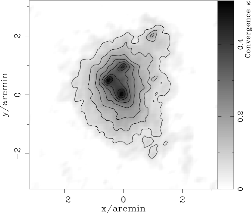
Figure 2: Dimensionless surface mass density $\kappa$ obtained by combining shear and flexion data in Fourier space (see equation [28]). The lowest contour and the contour interval are $\Delta\kappa=0.06$,

We estimated the unlensed dispersions of HOLICs to be $\sigma_{\zeta}\equiv\sqrt{\langle|\zeta|^{2}\rangle}\approx 0.0215\,{\rm arcsec}^{-1}$ and $\sigma_{\delta}\equiv\sqrt{\langle|\delta|^{2}\rangle}\simeq 0.0248\,{\rm arcsec}^{-1}$, where noisy outliers responsible for the non-Gaussian tail were removed in the variance estimation. After clipping rejections the number of galaxies in this “clean sample” is about $N_{\rm clean}\approx 3.1\times 10^{5}$ ($\bar{n}_{g}\approx 11\,{\rm arcmin}^{-2}$), and the median value of $r_{h}$ is $\langle r_{h}^{*}\rangle\approx 0\farcs 639$. Using the clean sample we also measured dispersions of dimensionless HOLICs, $a\zeta$ and $a\delta$, with $a$ being the characteristic scale of the observed galaxy (Goldberg & Bacon 2005; Goldberg & Leonard 2006). We take $a$ to be the half-light diameter, $a=2r_{h}$, while Goldberg & Bacon (2005) and Goldberg & Leonard (2006) chose $a$ to be the semimajor axis for measuring the intrinsic flexion of galaxies. We found $\sigma_{a\zeta}=0.0286$ and $\sigma_{a\delta}=0.0344$ with the median size of $\langle a\rangle_{\rm med}=1\farcs 27$. We note that there is a good agreement between $\sigma_{a\zeta}/\langle a\rangle_{\rm med}$ ($\sigma_{a\delta}/\langle a\rangle_{\rm med}$) and $\sigma_{\zeta}$ ($\sigma_{\delta}$), indicating that the measured dispersions are effectively weighted by moderately large galaxies with $a\approx 1^{\prime}$. The first HOLICs $\zeta$, which is a spin-1 quantity, is sensitive to the determination of the centroid, or the first moment, with spin-1. Thus the error in the centroid determination affects seriously the estimation of the first HOLICs $\zeta$, while this effect is of second order for other shape quantities with non spin-1 quantities. Note that even though small objects were excluded from the analysis, no anisotropic/isotropic PSF corrections were applied in measuring the HOLICs for the present study, which implies that the dispersions of HOLICs were underestimated to some degree due to the isotropic smearing effect by the atmosphere and the Gaussian weighting in $q[I(\mbox{\boldmath$\theta$})]$ (see Fig. 2 of Irwin et al. 2006).

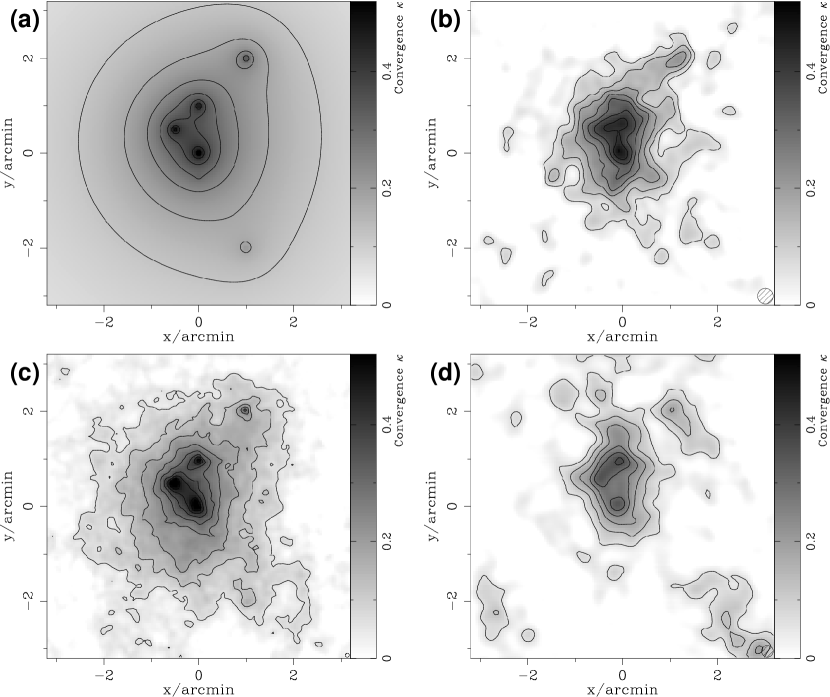
Figure 1: Reconstructions of the dimensionless surface mass density $\kappa$ of a model cluster at $z_{d}=0.1$ from simulated ellipticity and HOLICs data. The side length is 6.4 arcmin, and $4,096$ ($n_{g}=100\,{\rm arcmin}^{-}2$ ) randomly generated galaxies at a redshift of $z_{s}=1.2$ have been used for reconstructions (see §4). Shown in the top-left panel is the input $\kappa$ map of the model cluster. The top-right panel shows a $\kappa$ map reconstructed from image ellipticities, $\chi$. The bottom panels show $\kappa$ maps reconstructed using HOLICs, (c) $\zeta$ and (d) $\delta$. The lowest contour and the contour interval are $\Delta\kappa=0.06$. The shaded circle in each panel indicates the FWHM of the Gaussian filter.

In the present study, we simply adopt for illustration purposes random Gaussian distributions with dispersions of $\sigma_{\zeta}^{(s)}=\sigma_{\delta}^{(s)}=0.02\,{\rm arcsec}^{-1}$ in generating the intrinsic values of HOLICs, corresponding to flexion dispersions of $\sigma_{F}^{(s)}\simeq 0.009\,{\rm arcsec}^{-1}$ and $\sigma_{G}^{(s)}\simeq 0.027\,{\rm arcsec}^{-1}$. We note that Bacon et al. (2006) adopted $\sigma_{F}^{(s)}=\sigma_{G}^{(s)}=0.04\,{\rm arcsec}^{-1}$ in their simulation. For the intrinsic dispersion of ellipticities, we adopt $\sigma_{\chi}^{(s)}=0.4$. As a lens model we use a mock cluster located at $z_{d}=0.1$, which is shown as the dimensionless surface mass density $\kappa$ in the top-left panel of Fig. 1. The cluster consists of a main halo and five sub-halos which are described by NFW density profiles with different masses and concentration parameters. The field is square-shaped with a side length of $6.4$ arcmin. We use $N_{s}=4,096$ sources ($n_{g}=100\,{\rm arcmin}^{-2}$) randomly distributed over the field, with intrinsic shape quantities $(\chi^{(s)},\zeta^{(s)},\delta^{(s)})$ drawn from random Gaussian distributions with dispersion $(\sigma_{\chi}^{(s)},\sigma_{\zeta}^{(s)},\sigma_{\delta}^{(s)})$, respectively. We assume the background sources are located at a single redshift of $z_{s}=1.2$, which is a fair approximation for the lens located at a low redshift of $z_{d}=0.1$. These observation parameters are appropriate for a future space-based survey such as the planned weak lensing survey with the SNAP satellite (Massay et al. 2004), except that the intrinsic flexion dispersions $(\sigma_{F}^{(s)},\sigma_{G}^{(s)})$ are derived from ground-based weak lensing data with galaxies of $a=2r_{h}\approx 1^{\prime\prime}$. Hence the values of $(\sigma_{F}^{(s)},\sigma_{G}^{(s)})$ adopted in the present study will probably be very optimistic for space-based data with distant galaxies of $a\sim 0\farcs 5$ (see Fig. 2 of Massey et al. 2004). Such small, distant galaxies will have intrinsic flexion dispersions greater by a factor of a few. Finally, we use equations (7), (41), and (42) to generate lensed quantities $(\chi,\zeta,\delta)$ for all sources.

Figure 1 shows reconstructed mass maps of the model cluster using $(\chi,\zeta,\delta)$ along with the input mass model. We used the linear inversion equations (9), (26), and (27). The reconstructed $\kappa$-maps were smoothed with a Gaussian filter, where the Gaussian FWHMs are taken to be $(0\farcm 333,0\farcm 083,0\farcm 249)$ for reconstructions using $(\gamma,F,G)$, respectively. Then, the dispersions in the Gaussian-smoothed $B$-mode maps are obtained as $(\sigma_{B}(\gamma),\sigma_{B}(F),\sigma_{B}(G))=(0.0284,0.0236,0.0570)$. The $\kappa$ maps reconstructed using HOLICs recover substructures better than large-scale structures, allowing a high-resolution mass reconstruction. The superior sensitivity of flexion to small scale structure comes from the $1/k^{2}$-dependence of the noise power spectrum in a $\kappa$ reconstruction (see equation [29]). Further, since we have assumed $\sigma^{(s)}_{\zeta}=\sigma^{(s)}_{\delta}$ whereas $\zeta$ has a three-times larger response to flexion than $\delta$, the ${\cal F}$-based reconstruction has a three-times better sensitivity than the $\cal G$-based reconstruction.

In Fig. 2 we show the $\kappa$ map obtained by combining shear- and flexion-based reconstructions using equation (28). On small angular scales the signal is dominated by flexion, while it is dominated by gravitational shear on large angular scales. Since $\hat{W}_{\kappa F}(\mbox{\boldmath$k$})>\hat{W}_{\kappa G}(\mbox{\boldmath$k$})$ for all wavenumbers, the $\kappa$ map is less weighted by the second flexion for the observation parameters adopted in this study (i.e., $\sigma_{\zeta}=\sigma_{\delta}$). The rms noise level in the $\kappa$-map from flexion and shear data is reduced down to

$$\sigma_{B}\approx\frac{1}{\sqrt{\sum_{j=\gamma,F,G}1/\sigma^{2}_{B}(j)}}=0.0173.$$ (50)

5 Discussion and Conclusions

In the present paper, we have studied the possibility to improve the weak lensing analysis by utilizing the octopole and higher-multipole moments of lensed images that carries the third-order weak lensing effect. By defining proper combinations of octopole moments as HOLICs, we have derived explicit relations between the flexion fields $(F,G)$ and observable HOLICs $(\zeta,\delta)$. In the weak lensing limit, the first flexion $F$ excites in lensed images the first HOLICs $\zeta$ with spin-1, while the second flexion $G$ excites the second HOLICs $\delta$ with spin-3. One can employ the assumption of random orientation for intrinsic HOLICs of background sources to obtain an unbiased, direct estimator for flexion, in a similar manner to the usual prescription for weak lensing.

We have also shown by using simulated observations how the use of HOLICs can improve the accuracy and resolution of a reconstructed mass map, in which we assumed Gaussian uncertainties in the shape measurements estimated using deep $i^{\prime}$-band data of blank fields observed with Subaru/Suprime-Cam. The gravitational shear and flexion have different scale-dependence in mass reconstruction errors. The mass maps reconstructed using HOLICs recover substructures better than the shear-based reconstruction, allowing a high-resolution mass reconstruction. It is shown that an optimal linear combination of individual mass reconstructions can be formed using the statistical weight in Fourier space, which can improve the statistical significance of weak lensing mass reconstructions. In actual observations, on the other hand, we must apply various shape corrections (e.g., isotropic/anisotropic PSF corrections) to the higher order shape quantities in order to measure flexion to high precision. In particular, the first HOLICs $\zeta$ with spin-1 is highly sensitive to the choice of the center-of-image. These issues will be discussed further in the forthcoming publications.

Appendix A: Calculation of the Jacobian

We present detailed calculations of the Jacobian (29) in this appendix. Using the lens equation the Jacobian can be calculated as follows:

$$d^{2}\beta = {\rm det}\left(\begin{array}[]{cc}\partial\beta_{1}/\partial\theta_{1}&\partial\beta_{1}/\partial\theta_{2}\\ \partial\beta_{2}/\partial\theta_{1}&\partial\beta_{2}/\partial\theta_{2}\\ \end{array}\right)d^{2}\theta$$

$$= \Biggl{(}\left({\cal A}_{11}+{\cal D}_{111}d\theta_{1}+{\cal D}_{112}d\theta_{2}\right)\left({\cal A}_{22}+{\cal D}_{122}d\theta_{1}+{\cal D}_{222}d\theta_{2}\right)-\left({\cal A}_{12}+{\cal D}_{112}d\theta_{1}+{\cal D}_{122}d\theta_{2}\right)^{2}\Biggr{)}d^{2}\theta$$

$$\approx (1-\kappa)^{2}\times$$

$$\left(1-g-\frac{1}{2}(3F_{1}+G_{1})d\theta_{1}-\frac{1}{2}(F_{2}+G_{2})d\theta_{2}\right)\left(1+g-\frac{1}{2}(F_{1}-G_{1})d\theta_{1}-\frac{1}{2}(3F_{2}-G_{2})d\theta_{2}\right)d^{2}\theta$$

$$\approx (1-\kappa)^{2}\left(1-2F_{1}d\theta_{1}-2F_{2}d\theta_{2}\right)d^{2}\theta.$$ (4)

Appendix B: Effect of the Centroid Shift

In a weak lensing analysis we quantify the shape of an image by measuring various moments of the surface brightness distribution $I(\mbox{\boldmath$\theta$})$, in which the moments are calculated with respect to the centroid of the image, or the center of light, defined by the first moments of $I(\mbox{\boldmath$\theta$})$:

$$\bar{\theta}_{i}\equiv\frac{\int\!d^{2}\theta\,\theta_{i}I(\mbox{\boldmath$\theta$})}{\int\!d^{2}\theta\,I(\mbox{\boldmath$\theta$})}.$$ (5)

However, in general, this apparent center can be different from the “point” that is mapped using the lens equation from the center of unlensed light. We refer to this point as the “true” center of the image. The difference between these two centers, namely the apparent and the true centers, cause a significant effect in evaluating the first flexion as pointed out by Goldberg & Bacon (2005). For the second flexion the effect of the centroid shift is second order so that we will ignore it in the present paper.

Let us define the center of the source in the absence of gravitational lensing as $\bar{\beta}_{i}$ and the apparent center of the lensed image as $\bar{\theta}_{i}$. We also define the true center of the image that is mapped from $\bar{\beta}_{i}$ using the lens equation, as $\theta_{i}(\bar{\mbox{\boldmath$\beta$}})$. Similarly, we define the point in the source plane that is inversely mapped by the lens equation from $\bar{\theta}_{i}$ as $\beta_{i}(\bar{\mbox{\boldmath$\theta$}})$. Then, we have

$$\beta_{i}(\bar{\mbox{\boldmath$\theta$}})-\bar{\beta}_{i} = \bar{\theta}_{i}-\alpha_{i}(\bar{\mbox{\boldmath$\theta$}})-\bar{\beta}_{i}=\bar{\theta}_{i}-\alpha_{i}(\bar{\mbox{\boldmath$\theta$}})-\frac{\int\!d^{2}\beta\,\beta_{i}I^{s}(\mbox{\boldmath$\beta$})}{\int\!d^{2}\beta\,I^{s}(\mbox{\boldmath$\beta$})}$$ (6)

$$= \bar{\theta}_{i}-\alpha_{i}(\bar{\mbox{\boldmath$\theta$}})-\frac{\int\!d^{2}\theta\,(1-2F_{j}d\theta_{j})\left(\theta_{i}-\alpha_{i}(\mbox{\boldmath$\theta$})\right)I(\mbox{\boldmath$\theta$})}{\int\!d^{2}\theta\,(1-2F_{j}d\theta_{j})I(\mbox{\boldmath$\theta$})}$$

where we have used the expression (Appendix A: Calculation of the Jacobian) for the Jacobian and used the relation between the lensed and unlensed surface brightness distributions, $I(\mbox{\boldmath$\theta$})=I^{s}(\mbox{\boldmath$\beta$})$, with $\beta_{i}=\theta_{i}-\alpha_{i}(\mbox{\boldmath$\theta$}_{i})$. We then expand the deflection angle $\alpha_{i}$ in equation (6) as

$$\alpha_{i}(\mbox{\boldmath$\theta$})\approx\alpha_{i}(\bar{\mbox{\boldmath$\theta$}})+\alpha_{i,j}d\theta_{j}+\frac{1}{2}\alpha_{i,jk}d\theta_{j}d\theta_{k}=\alpha_{i}(\bar{\mbox{\boldmath$\theta$}})-\left({\cal A}-{\bf 1}\right)_{ij}d\theta_{j}-\frac{1}{2}{\cal D}_{ijk}d\theta_{j}d\theta_{k}$$ (7)

with $\theta_{i}=\bar{\theta}_{i}+d\theta_{i}$. Thus, in the first order of the gravitational shear and flexion, we have

$$\beta_{i}(\bar{\mbox{\boldmath$\theta$}})-\bar{\beta}_{i} = \bar{\theta}_{i}-\alpha_{i}(\bar{\mbox{\boldmath$\theta$}})$$ (8)

$$-\frac{\int\!d^{2}\theta\,(1-2F_{l}d\theta_{l})\left(\bar{\theta}_{i}+d\theta_{i}-\alpha_{i}(\bar{\mbox{\boldmath$\theta$}})+\left({\cal A}-{\bf 1}\right)_{ij}d\theta_{j}+\frac{1}{2}{\cal D}_{ijk}d\theta_{j}d\theta_{k}\right)I(\mbox{\boldmath$\theta$})}{\int\!d^{2}\theta\,(1-2F_{l}d\theta_{l})I(\mbox{\boldmath$\theta$})}$$

$$= \frac{\int\!d^{2}\theta\,(1-\kappa)2F_{l}d\theta_{l}d\theta_{i}I(\mbox{\boldmath$\theta$})}{\int\!d^{2}\theta\,I(\mbox{\boldmath$\theta$})}-\frac{1}{2}\frac{\int\!d^{2}\theta\,{\cal D}_{ijk}d\theta_{j}d\theta_{k}I(\mbox{\boldmath$\theta$})}{\int\!d^{2}\theta\,I(\mbox{\boldmath$\theta$})}$$

$$= {\rm tr}Q\left(\frac{3}{2}{\cal F}_{i}+\frac{5}{4}[{\cal F}^{*}\chi]_{i}+\frac{1}{4}[{\cal G}\chi^{*}]_{i}\right),$$

where ${\rm tr}Q=Q_{11}+Q_{22}$ is the trace of $Q_{ij}$ defined by equation (5). Thus the displacement from the true to the apparent center is ${\rm tr}Q\left(\frac{3}{2}{\cal F}_{i}+\frac{5}{4}[{\cal F}^{*}\chi]_{i}+\frac{1}{4}[{\cal G}\chi^{*}]_{i}\right)$ in the “source plane”, and all of the shape quantities in equation (8) are measured using the apparent center $\bar{\mbox{\boldmath$\theta$}}$. In the zeroth order of the shear and flexion, this displacement is magnified by $1/(1-\kappa)$ in the image plane, so that we have

$$\theta_{i}(\bar{\mbox{\boldmath$\beta$}})\approx\bar{\theta}_{i}-{\rm tr}Q\left(\frac{3}{2}F_{i}+\frac{5}{4}[F^{*}\chi]_{i}+\frac{1}{4}[G\chi^{*}]_{i}\right)$$ (9)

where $F$ and $G$ are the first and the second flexion, $F={\cal F}/(1-\kappa)$ and $G/(1-\kappa)$.

Next, we evaluate the effect of the centroid shift for measuring the first HOLICs, $\zeta$. We define the apparent octopole moments (with respect to the apparent center $\bar{\mbox{\boldmath$\theta$}}$) as

$$Q_{ijk}=\frac{\int\!d^{2}\theta\,d\theta_{i}d\theta_{j}d\theta_{k}I(\mbox{\boldmath$\theta$})}{\int\!d^{2}\theta\,I(\mbox{\boldmath$\theta$})}$$ (10)

and the “true” octopole moments (with respect to the true center $\mbox{\boldmath$\theta$}(\bar{\beta})$) as

$$Q^{t}_{ijk} = \frac{\int\!d^{2}\theta\,\left(\theta_{i}-\theta_{i}(\bar{\mbox{\boldmath$\beta$}})\right)\left(\theta_{j}-\theta_{j}(\bar{\mbox{\boldmath$\beta$}})\right)\left(\theta_{k}-\theta_{k}(\bar{\mbox{\boldmath$\beta$}})\right)I(\mbox{\boldmath$\theta$})}{\int\!d^{2}\theta\,I(\mbox{\boldmath$\theta$})}$$ (11)

$$= \frac{\int\!d^{2}\theta\,(d\theta_{i}+\Delta^{\theta}_{i})(d\theta_{j}+\Delta^{\theta}_{j})(d\theta_{k}+\Delta^{\theta}_{k})I(\mbox{\boldmath$\theta$})}{\int\!d^{2}\theta\,I(\mbox{\boldmath$\theta$})}$$ (12)

where $\Delta^{\theta}_{i}={\rm tr}Q\left(\frac{3}{2}F_{i}+\frac{5}{4}[F^{*}\chi]_{i}+\frac{1}{4}[G\chi^{*}]_{i}\right)$. Using the expressions for the moments above, it is straightforward to calculate the corresponding HOLICs using the moments with respect to the true center, and then to have the relation between $\zeta^{t}$ constructed using the true center and $\zeta$ constructed using the apparent center:

$$\zeta^{t}=\zeta+2\frac{{\rm tr}Q}{\xi}\Delta^{\theta}+\frac{{\rm tr}Q}{\xi}[\chi\Delta^{\theta*}]\approx\zeta+\frac{\left({\rm tr}Q\right)^{2}}{\xi}\left(3F+4F^{*}\chi+\frac{1}{2}G\chi^{*}\right)$$ (13)

as well as the relation between $\delta^{t}$ and $\delta$:

$$\delta^{t}=\delta+3\frac{{\rm tr}Q}{\xi}[\chi\Delta^{\theta}]\approx\delta+\frac{9}{2}\frac{\left({\rm tr}Q\right)^{2}}{\xi}\chi F,$$ (14)

up to the the second order of the shear, flexion and non 0-spin shape quantities. Equations (13) and (14) allow us to establish the required relationships between the unlensed HOLICs $(\zeta^{(s)},\delta^{(s)})$ and the lensed HOLICs $(\zeta,\delta)$ (note that equations [41] and [42] are the relations between $\zeta^{(s)}$ and $\zeta^{t}$, and between $\delta^{(s)}$ and $\delta^{t}$, respectively, in the notation of this appendix),

$$\zeta^{(s)} = \frac{\zeta-2g\zeta^{*}-g^{*}\delta-\frac{1}{4}(8F^{*}\eta-16\frac{\left({\rm tr}Q\right)^{2}}{\xi}F^{*}\chi+9F-12\frac{\left({\rm tr}Q\right)^{2}}{\xi}F+2G\eta^{*}-2\frac{\left({\rm tr}Q\right)^{2}}{\xi}G\chi^{*}+G^{*}\lambda)}{(1-\kappa)(1-4Re[g^{*}\lambda]-5Re[F\iota_{I}^{*}]-Re[G\iota_{III}^{*}])},$$ (15)

$$\delta^{(s)} = \frac{\delta-3g\zeta-\frac{1}{4}(10F\eta-18\frac{\left({\rm tr}Q\right)^{2}}{\xi}F\chi+7F^{*}\lambda+3G)}{(1-\kappa)(1-4Re[g^{*}\lambda]-5Re[F\iota_{I}^{*}]-Re[G\iota_{III}^{*}])}.$$ (16)

Finally, in the first order, the first flexion is expressed using the observable shape quantities as

$$\langle\zeta\rangle\approx\left(\frac{9}{4}-3\left<\frac{({\rm tr}Q)^{2}}{\xi}\right>\right)\,F.$$ (17)

One can see the asymptotic behavior of the correction term in equation (17), when the lensed image is close to a circle. For an image with the circular top-hat brightness profile, we have $({\rm tr}Q/\xi)^{2}=3/4$, so that one will measure $\zeta=0$ regardless of the value of $F$.

References

- (1) Bacon, D. J., Goldberg, D. M., Rowe, B. T. P., & Taylor, A. N. 2006, MNRAS, 365, 414
- (2) Bartelmann, M., & Schneider, P. 2001, Phys.Rep., 340, 291
- (3) Goldberg, D. M., & Natarajan, P. 2002, ApJ, 564, 65
- (4) Goldberg, D. M., & Bacon, D. J. 2005, ApJ, 619, 741
- (5) Gldberg, D. M., & Leonard, A. 2006, ApJ, accepted
- (6) Irwin, J., & Shmakova, M. 2006, ApJ, 645, 17
- (7) Irwin, J., Shmakova, M., & Anderson, J. 2006, astro-ph/0607007
- (8) Kaiser, N.. Squires, G., Broadhurst, T. 1995, ApJ, 449, 460
- (9) Massey, R. et al. 2004, AJ, 127, 3089
- (10) Massey, R. & Refregier, A. 2005, MNRAS, 363, 197M
- (11) Refregier, A. 2003, MNRAS, 338, 35
- (12) Refergier, A., & Bacon, D. 2003, MNRAS, 338, 48
- (13) Scoville, N. et al. 2007, to appear in COSMOS ApJ Suppl. special issue (astro-ph/0612306)