Neutrino signatures of supernova turbulence

Abstract

Convection that develops behind the shock front during the first second of a core-collapse supernova explosion is believed to play a crucial role in the explosion mechanism. We demonstrate that the resulting turbulent density fluctuations may be directly observable in the neutrino signal starting at $t\gtrsim 3-4$ s after the onset of the explosion. The effect comes from the modulation of the MSW flavor transformations by the turbulent density fluctuations. We derive a simple and general criterion for neutrino flavor depolarization in a Kolmogorov-type turbulence and apply it to the turbulence seen in modern numerical simulations. The turbulence casts a “shadow”, by making other features, such as the shock front, unobservable in the density range covered by the turbulence.

I Introduction

The leading proposal for the mechanism of core-collapse supernova explosions is that the shock first stalls and then regains its energy through heating of the material behind it by streaming neutrinos ColgateWhite1966 ; Wilson1985 . Within this paradigm a crucial role is played by vigorous convection behind the shock front Bethe1990 ; HerantColgate1994 . This convection, clearly seen in modern multidimensional simulations FryerWarren2003 ; JankaPRL ; Kifonidis:2005yj ; Scheck:2006rw ; Burrowsacoustic , brings the energy deposited by neutrinos in dense regions to the region behind the stalled shock front (for a recent overview and references see, e.g., WoosleyJanka ). Besides the shock revival, the convection leads to asymmetric accretion onto the protoneutron star, providing a compelling explanation for the high observed pulsar velocities JankaPRL . Finally, evidence for the convection comes from observations of SN1987A that indicate extensive mixing during the early stages of the explosion HerantBenz1992 .

Turbulent convective motions create a fluctuating density field in the post-shock region. Importantly, these fluctuations remain long after the shock restarts and a successful explosion is obtained Kifonidis:2005yj ; Scheck:2006rw . In particular, they persist over the duration of the neutrino burst ($\sim 10$ sec) and can thus modulate the MSW flavor transformations of the neutrinos. The goal of the present work is to show that the turbulence seen in the simulations indeed leaves an imprint on the neutrino signal, possibly starting from about 3-4 seconds after the onset of the explosion. This imprint may replace, or combine with, signatures of other features already discussed in the literature, such as the passage of the front SchiratoFuller and reverse RaffeltDighe shocks through the resonance layer (see also Lisi2004 ), or effects of low-density bubbles KnellerMcLaughlin .

II Outline

A core-collapse supernova emits both neutrinos and antineutrinos, of all three flavors, with energies $\sim$10-20 MeV. The spectra and luminosities for $\nu_{e}$, $\bar{\nu}_{e}$, and $\nu_{x}$ ($x=\mu,\tau,\bar{\mu},\bar{\tau}$) are in general different. On the way out of the star, the neutrinos undergo matter-enhanced flavor transformations at certain characteristic (“resonant”) densities, $\rho_{H}\sim 2.4\times 10^{3}$ g/cm³ $(15\mbox{ MeV}/E_{\nu})(0.5/Y_{e})$ ($H$ or “high” resonance) and $\rho_{L}\sim\mbox{7}\times 10^{1}$ g/cm³ $(15\mbox{ MeV}/E_{\nu})(0.5/Y_{e})$ ($L$ or “low” resonance) . These transformations permute the neutrinos in various flavors and determine the neutrino spectra detected on Earth.

To estimate the effect of the turbulence on the permutation efficiency, we need to know the spectrum of the density fluctuations in the turbulence and the response of neutrino evolution to stochastic fluctuations of different sizes. The two tasks are tightly coupled. The fluctuations relevant to neutrino evolution turn out to be smaller than the resolution of the present simulations and, hence, must be inferred from the large-scale features seen in the simulations by physical arguments. At the same time, the spectrum of fluctuations in a physical turbulence is very different from the “$\delta$-correlated” noise for which analytical solutions for neutrino evolution exist Nicolaidis ; Loreti1994 ; Loreti:1995ae ; Balantekin1996 ; BurgessMichaud ; BurgessProceedings . The appropriate treatment will be developed here.

III Turbulence

As we will see, the scales of interest are $\lambda\lesssim 15/\sin 2\theta_{13}$ km. Unless $\sin 2\theta<10^{-3}$, these are much smaller than the local scale height $r$ at $t\gtrsim 4$ sec. Due to Rayleigh-Taylor and Kelvin-Helmholts instabilities, which are clearly seen in the simulations, Kolmogorov cascade into smaller scales should develop. Density (just like velocity) will then exhibit power-law fluctuations on all inertial range scales, that is on all scales between $r$ and viscous cut-off $l_{v}$ ($l_{v}\ll\lambda\ll r$),

$$C(k)\equiv\int dx\langle\delta n(0)\delta n(x)\rangle e^{-ikx}=C_{0}k^{\alpha}.$$ (1)

For the Kolmogorov turbulence the Fourier transform of the velocity correlator has $\alpha=-5/3$. We will consider the range $-2\lesssim\alpha\lesssim-1.5$.

Eq. (1) implies that a density variation between two points separated by a distance $\lambda$ scales as $\sim\left[\int_{2\pi/\lambda}^{2\pi/l_{v}}\frac{dk}{2\pi}C_{0}k^{\alpha}\right]^{1/2}$. For $\alpha>-1$ the variation has a strong unphysical dependence on the UV cutoff, $\propto l_{v}^{-(\alpha+1)/2}$, and diverges as $l_{v}\rightarrow 0$. This is obvious for the $\delta$-correlated noise, $\langle\delta n_{e}(x)\delta n_{e}(y)\rangle=const\times\delta(x-y)$, for which $\alpha=0$: the small-scale variation is infinite. Even if one tries to make sense of the $\delta$-correlated noise by imposing an ad-hoc UV cutoff, one has no connection with a realistic turbulence. On the contrary, $\alpha<-1$ is physical as everything is related to the fluctuations on the largest scales. Flavor transformations in a medium with this spectrum of the fluctuations, to the best of our knowledge, have not been treated in the literature .

IV Effects of fluctuations: a toy model

We consider a 2-flavor system which goes through a “noisy” level-crossing, with a Kolmogorov spectrum. We take the Hamiltonian

$$H_{2\nu}^{flavor} = \left(\begin{array}[]{cc}-\Delta\cos 2\theta+A(x)&\Delta\sin 2\theta\\ \Delta\sin 2\theta&\Delta\cos 2\theta-A(x)\end{array}\right),$$ (4)

with $\Delta\equiv\Delta m^{2}/4E_{\nu}$, $A(x)\equiv G_{F}n_{e}(x)/\sqrt{2}$, and set $\Delta=50$, $\theta=0.1$, $A(x)=x+A_{noise}(x)$. The noisy component of the profile is modelled as

$$A_{noise}(x)=F\sum_{k=1}^{600}k^{\beta}\cos[kx+\phi(k)],$$ (5)

where $F$ is a normalization factor, $\beta=\alpha/2=-5/6$ and $\phi(k)$ are random phases. The parameters are chosen such that for $F=0$ the evolution is adiabatic (the adiabaticity parameter $\gamma=\pi\Delta^{2}\sin^{2}2\theta/|A^{\prime}|\gg 1$), and the relevant range $k\geq 2\Delta\sin 2\theta=20$ (see later) is covered.

Let us compute the survival probability $P$ of a neutrino of a given flavor (for definiteness $\nu_{e}$) traveling from $x_{start}=-100$ to $x_{end}=100$ for different values of the noise amplitude $F$. Since the process is stochastic, for each $F$ we repeat the calculation with different random phases. The results are shown in Fig. 1. Three different regimes are clearly seen: (i) For small noise $(F\lesssim 10^{-2})$ its effects are negligible; $P(\nu_{e}\rightarrow\nu_{e})$ is dictated entirely by the smooth component of the profile. (ii) As the noise is increased, a stochastic scatter appears; from $F\sim 0.2$ to $1$ the average survival probability – shown by the diamonds – grows as a power law with $F$. (iii) Finally, for $F\gtrsim 1-2$, the average $P(\nu_{e}\rightarrow\nu_{e})$ saturates to $1/2$; any value of $P(\nu_{e}\rightarrow\nu_{e})$ in the interval $[0,1]$ is equally likely.

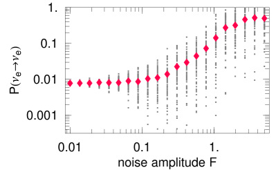
Figure 1: The electron neutrino survival probability as a function of the noise amplitude $F$ (see Eq. (5)). For each $F$, the calculation was repeated 66 times, with different random phases $\phi(k)$. The points indicate the results of individual runs, while the diamonds show the average values.

The saturation is easy to understand: in strongly fluctuating backgrounds, the final state expectation value $\langle\nu_{f}|\vec{\sigma}|\nu_{f}\rangle$ is equally likely to point in any direction in the flavor space. The averaged final state is described by a density matrix $diag(1/2,1/2)$: it is completely depolarized, all information about the initial state is lost. This result, well-known in the case of the $\delta$-correlated noise, is expected in general.

V Method of analysis

Fig. 1 suggests that to understand the impact of the density noise on neutrinos it is enough to derive the expression for $P(\nu_{e}\rightarrow\nu_{e})$ in the intermediate power-law regime. If the answer turns out to be $\gtrsim 1/2$, the noise completely flavor-depolarizes the neutrino state and the true answer is $P(\nu_{e}\rightarrow\nu_{e})=1/2$. Given the significant uncertainties in the explosion model, the problem may not warrant anything more elaborate.

VI Derivation of the effect of fluctuations

To begin, consider a smooth density profile $n_{0}(x)$. Rotate the Schrödinger equation, $i\phi^{\prime}=H(x)\phi$, with $H(x)$ of Eq. (4), to the basis $\psi(x)=V(x)\phi$ which diagonalizes the instantaneous Hamiltonian. The full Hamiltonian in the rotated basis has the form (see, e.g., myresonance for details)

$$H_{0}^{mass} = \left(\begin{array}[]{cc}-\Delta_{m}&-id\theta_{m}/dx\\ id\theta_{m}/dx&\Delta_{m}\end{array}\right),$$ (8)

where, introducing $A_{0}(x)\equiv G_{F}n_{0}(x)/\sqrt{2}$,

$$\Delta_{m} = [(\Delta\cos 2\theta-A_{0})^{2}+\Delta^{2}\sin^{2}2\theta]^{-1/2},$$ (9)

$$\sin 2\theta_{m} = \Delta\sin 2\theta/\Delta_{m}.$$ (10)

Now let us add a fluctuating density component $\delta n(x)$, so that $\delta A(x)\equiv G_{F}\delta n(x)/\sqrt{2}$. We again rotate the evolution equation to the instantaneous mass basis. Importantly, however, we choose the basic defined not by the total matter term, $A_{0}(x)+\delta A(x)$, but only $A_{0}(x)$. We have

$$i\psi^{\prime}=\left[H_{0}^{mass}(x)+\delta A\left(\begin{array}[]{cc}\cos 2\theta_{m}&\sin 2\theta_{m}\\ \sin 2\theta_{m}&-\cos 2\theta_{m}\end{array}\right)\right]\psi.$$ (11)

Transitions between the basis states are driven by the off-diagonal terms $id\theta_{m}/dx$ and $\delta A\sin 2\theta_{m}$. Assuming the evolution without the fluctuations would be adiabatic , we neglect the first of these terms and concentrate on the second. Moreover, we assume $\Delta_{m}(x)\gg\delta A(x)\cos 2\theta_{m}$, i.e. approximate the diagonal splitting by $2\Delta_{m}(x)$. Then, in the perturbative limit, the probability of a transition is

$$P \simeq \left|\int_{x_{i}}^{x_{f}}dx\delta A(x)\sin 2\theta_{m}(x)e^{i\int^{x}dx^{\prime}2\Delta_{m}(x^{\prime})}\right|^{2}.$$ (12)

Using Eq. (1), we get

$$P \simeq \frac{G_{F}^{2}}{2}\int\frac{dk}{2\pi}C(k)\left|\int_{x_{i}}^{x_{f}}dx\sin 2\theta_{m}(x)\right.$$ (13)

$$\times \left.\exp[i\int^{x}dx^{\prime}(2\Delta_{m}(x)-k)]\right|^{2}.$$

Let us explore the implications of this result. First, consider a turbulent density field superimposed on a constant smooth density, $A_{0}(x)=const$. After the neutrino travels a distance $L\gg\Delta_{m}^{-1}$, we have

$$P^{const}\simeq G_{F}^{2}L\sin^{2}2\theta_{m}C_{0}(2\Delta_{m})^{\alpha}/8.$$ (14)

The contributions come from a narrow interval of $k$, with the width of $\sim L^{-1}$, centered on $k_{0}=2\Delta_{m}$.

Eq. (14) says that: (i) The depolarization is efficient near the resonance, where $\sin 2\theta_{m}$ is large and $\Delta_{m}$ is small. (ii) The effect is proportional to $L$ and may be significant even off-resonance for a sufficiently extended turbulent region. We will investigate both in turn.

Consider now a resonance crossing with a linear smooth component, $A_{0}=A_{0}^{\prime}x$. The integral over $x$ in Eq. (13) can be approximately evaluated using a stationary phase method. For each $k>2\Delta\sin 2\theta_{13}$ there are two stationary points, which on physical grounds (e.g., integration over energy, variations in the profile) should be added incoherently. We obtain

$$P\simeq\frac{G_{F}}{\sqrt{2}n_{0}^{\prime}}\int dkC(k)G\left(\frac{k}{2\Delta\sin 2\theta}\right),$$ (15)

where the spectral weight $G(p)$ is given by

$$G(p)\simeq\Theta(p-1)p^{-1}(p^{2}-1)^{-1/2}.$$ (16)

The fluctuations that contribute have wavelengths $\leq 4\pi E_{\nu}/(\Delta m^{2}\sin 2\theta)$, or, for the $H$-resonance, $\leq 47$ km $\times(E_{\nu}/15$ MeV)$(0.3/\sin 2\theta_{13})$.

For power-law $C(k)$ in Eq. (1) the integral in Eq. (15) can be evaluated analytically,

$$P^{power-law}\simeq\frac{G_{F}C_{0}}{\sqrt{2}|n_{0}^{\prime}|}(2\Delta\sin 2\theta_{13})^{\alpha+1}\times N,$$ (17)

where the order one numerical coefficient $N$ is given by $N=\sqrt{\pi}\Gamma\left(1/2-\alpha/2\right)/[2\Gamma\left(1-\alpha/2\right)]$.

For the $\delta$-correlated noise ($\alpha=0$) Eq. (17) gives

$$P^{\delta-corr}\simeq\pi G_{F}C_{0}\Delta\sin 2\theta_{13}/\sqrt{2}|n_{0}^{\prime}|.$$ (18)

This agrees with the known result, expanded in the same perturbative limit. In the physically interesting case of the Kolmogorov spectrum $(\alpha=-5/3)$, we get $N=\sqrt{\pi}\Gamma(4/3)/2\Gamma(11/6)\approx 0.84$ and

$$P^{Kolm}\simeq 0.84G_{F}C_{0}(2\Delta\sin 2\theta_{13})^{-2/3}/\sqrt{2}|n_{0}^{\prime}|.$$ (19)

Eq. (19) reproduces the power-law rise seen in Fig. 1.

VII Application to the supernova

Let us apply Eq. (19) to the actual supernova case. Four seconds into the explosion (Kifonidis:2005yj , Fig. 4a), when the shock expands to $L\simeq 5\times 10^{4}$ km, the density in parts of the turbulent region drops to that of the $H$ resonance . Estimating $|n_{0}^{\prime}|$ as $\sim n_{0}/L$ and using $n_{0}=\sqrt{2}\Delta/G_{F}$ and $\delta n_{L}^{2}\sim C_{0}(2\pi/L)^{\alpha+1}/[2\pi|\alpha+1|]$, we write the depolarization criterion ($P\gtrsim 1/2$, with $P$ from Eq. (19)) as

$${\delta n_{L}/n_{L}}>\tilde{f}~{}\theta_{13}^{-(\alpha+1)/2}(\Delta L)^{-(\alpha+2)/2},$$ (20)

where $\tilde{f}=\sqrt{\pi^{\alpha}/[N|\alpha+1|2^{\alpha+3}]}$ is an order one factor.

For Kolmogorov’s $\alpha=-5/3$, we get

$${\delta n_{L}/n_{L}}>0.07~{}\theta_{13}^{1/3}.$$ (21)

Fig.4a of Kifonidis:2005yj shows that inside the turbulent region $\delta n_{L}/n_{L}\sim$ a few. Thus, the depolarization criterion is actually satisfied, and by a large margin. Importantly, this result is robust to variations in the details of the turbulent spectrum. As $\alpha$ is varied from $-2$ to $-1.5$, the numerical factor in (21) varies only from 0.04 to 0.25.

VIII Off-resonance depolarization

By continuity, depolarization must be present even before the density reaches its resonant value . Let us estimate at what point the depolarization effect becomes significant. One way is to model the post-shock profile as a constant density region of extent $L\sim\mbox{a few}\times 10^{9}$ cm. Using Eq. (14) with $\sin 2\theta_{m}=\Delta\sin 2\theta/\Delta_{m}$, $G_{F}^{2}C_{0}/2\sim A_{0}^{2}/k^{\alpha+1}=A_{0}^{2}(L/2\pi)^{\alpha+1}$ and $\Delta_{m}\simeq(A_{0}-\Delta)$, we get

$$P^{const}\sim L^{\alpha+2}\Delta^{2}\sin^{2}2\theta_{13}A_{0}^{2}(A_{0}-\Delta)^{\alpha-2}/8\pi^{\alpha+1}.$$ (22)

Plugging in $E_{\nu}=1.5\times 10^{7}$ eV and $L\sim 2.5\times 10^{14}$ eV^-1 we find that $P=0.1$ is obtained when the density is 4 times the resonant value for $\sin^{2}2\theta_{13}\sim 0.1$; 2 times the resonant value for $\sin^{2}2\theta_{13}\sim 0.01$; and 1.5 times the resonant value for $\sin^{2}2\theta_{13}\sim 0.001$. To interpret these numbers, we consult, e.g., Fig. 2 of RaffeltDighe where contours of constant density are shown as a function of time for a one-dimensional model of an exploding supernova. We see that for $0.01\lesssim\sin^{2}2\theta_{13}\lesssim 0.1$ significant ($P\sim 0.1$) depolarization occurs already at $t=3$ sec.

To check the robustness of this result to the details of the profile, we can also model the smooth component $A_{0}(x)$ in the post-shock region by a parabola, $A_{0}(x)=a+bx^{2}/2$. In the far-off-resonance limit, $a-\Delta\gg\Delta\sin 2\theta_{13}$, we get from Eq. (13)

$$P^{parab}\simeq N_{2}\frac{\Delta^{2}\sin^{2}2\theta_{13}}{\sqrt{b}}G_{F}^{2}C_{0}(a-\Delta\cos\theta_{13})^{\alpha-\frac{3}{2}},$$ (23)

where $N_{2}=2^{\alpha-1/2}\sqrt{\pi}\Gamma(3/2-\alpha)/\Gamma(2-\alpha)$. Eq. (23) yields an estimate that is quite similar to the one obtained using Eq. (22) .

IX Experimental implications

Let us briefly list the experimental implications of our findings.

(1) When the densities in the turbulence reach $\mbox{a few}\times 10^{3}$ g/cm³, assuming $\sin^{2}2\theta_{13}\gtrsim 10^{-3}$, the $H$-resonance should become completely flavor-depolarized. This manifests itself in a characteristic dip of the average energy in the detector, or changing rate of the high-energy events. This is qualitatively (but not quantitatively) similar to what has been discussed in connection with the passage of the front shock RaffeltDighe . Just like in that case, the signature appears either in neutrinos or antineutrinos, depending on the sign of the neutrino mass hierarchy. An observation of the effect would thus determine the sign of the mass hierarchy and place a lower bound on $\theta_{13}$.

(2) The onset of the depolarization would be gradual, with the off-resonance effects possibly present up to a second earlier. This may be used to distinguish turbulence from the shock effects, as the latter are more abrupt. The effect may be even more pronounced for the $L$ resonance.

(3) The depolarization replaces the signatures of the front shock and other features in the density range covered by the turbulence. Indeed, flavor-depolarized neutrino is described by a density matrix $diag(1/2,1/2)$, which commutes with any Hamiltonian and carries no information about density features either before or after the turbulence. This extends to the Earth effect when the $L$ resonance also becomes depolarized, providing yet another possible way to distinguish turbulence from other effects at future large detectors. The observation about the loss of sensitivity to the front shock was also made in an interesting recent paper Lisi2006 . Unfortunately, Lisi2006 considers an ad-hoc $\delta$-correlated noise, following Nicolaidis ; Loreti1994 ; Loreti:1995ae ; Balantekin1996 ; BurgessMichaud ; BurgessProceedings .

(4) The density profile varies between models and, moreover, even within a given model Kifonidis:2005yj varies significantly depending on the direction to the observer. Consequently, there is no unique prediction for when exactly the depolarization effects appear first.

A detailed study of experimental signatures in various scenarios (different hierarchies, ranges of $\theta_{13}$, explosion models) will be published elsewhere.

- (1) S. Colgate and R. White, Astrophys. J. 143, 626 (1966).
- (2) J. R. Wilson, in Numerical astrophysics, edited by J. M. Centrella, J. M. LeBlanc, and R. L. Bowers, Jones & Bartlett, Boston (1985).
- (3) H. A. Bethe, Rev. Mod. Phys. 62, 801 (1990).
- (4) M. Herant, W. Benz, W. R. Hix, C. L. Fryer and S. A. Colgate, Astrophys. J. 435, 339 (1994).
- (5) C. L. Fryer and M. S. Warren, Astrophys. J. 601, 391 (2004) [arXiv:astro-ph/0309539].
- (6) K. Kifonidis, T. Plewa, L. Scheck, H. T. Janka and E. Mueller, arXiv:astro-ph/0511369.
- (7) L. Scheck, K. Kifonidis, H. T. Janka and E. Mueller, arXiv:astro-ph/0601302.
- (8) L. Scheck, T. Plewa, H. T. Janka, K. Kifonidis and E. Mueller, Phys. Rev. Lett. 92, 011103 (2004).
- (9) A. Burrows, E. Livne, L. Dessart, C. Ott and J. Murphy, arXiv:astro-ph/0510687.
- (10) S. Woosley and T. Janka, Nature Physics 1, 147 (2005).
- (11) M. Herant and W. Benz, Astrophys. J. 387, 294 (1992).
- (12) R. C. Schirato, G. M. Fuller, arXiv:astro-ph/0205390.
- (13) R. Tomas, M. Kachelriess, G. Raffelt, A. Dighe, H. T. Janka and L. Scheck, JCAP 0409, 015 (2004).
- (14) G. L. Fogli, E. Lisi, A. Mirizzi and D. Montanino, JCAP 0504, 002 (2005) [arXiv:hep-ph/0412046].
- (15) J. P. Kneller and G. C. McLaughlin, Phys. Rev. D 73, 056003 (2006) [arXiv:hep-ph/0509356].
- (16) T. Araki et al. [KamLAND Collaboration], Phys. Rev. Lett. 94, 081801 (2005) [arXiv:hep-ex/0406035].
- (17) A. Friedland and C. Lunardini, arXiv:hep-ph/0606101.
- (18) A. Friedland, Phys. Rev. D 64, 013008 (2001).
- (19) A. Nicolaidis, Phys. Lett. B 262, 303 (1991).
- (20) F. N. Loreti and A. B. Balantekin, Phys. Rev. D 50, 4762 (1994) [arXiv:nucl-th/9406003].
- (21) A. B. Balantekin, J. M. Fetter and F. N. Loreti, Phys. Rev. D 54, 3941 (1996) [arXiv:astro-ph/9604061].
- (22) C. P. Burgess and D. Michaud, Annals Phys. 256, 1 (1997) [arXiv:hep-ph/9606295].
- (23) C. P. Burgess and D. Michaud, arXiv:hep-ph/9611368.
- (24) F. N. Loreti, Y. Z. Qian, G. M. Fuller and A. B. Balantekin, Phys. Rev. D 52, 6664 (1995).
- (25) A. S. Dighe and A. Y. Smirnov, Phys. Rev. D 62, 033007 (2000), hep-ph/9907423; C. Lunardini and A. Y. Smirnov, JCAP 0306, 009 (2003) hep-ph/0302033.
- (26) W. Haxton and W. Zhang, Phys. Rev. D 43, 2484 (1991).
- (27) O. G. Miranda, T. I. Rashba, A. I. Rez and J. W. F. Valle, Phys. Rev. D 70, 113002 (2004) [arXiv:hep-ph/0406066].
- (28) A. Friedland, arXiv:hep-ph/0505165.
- (29) E. Kh. Akhmedov, Yad. Fiz. 47 475 (1988) [Sov. J. Nucl. Phys. 47 301 (1988)].
- (30) G. L. Fogli, E. Lisi, A. Mirizzi and D. Montanino, arXiv:hep-ph/0603033.