The XMM Large Scale Structure survey:
The X-ray pipeline and survey selection function

Abstract

We present the X-ray pipeline developed for the purpose of the cluster search in the XMM-LSS survey. It is based on a two-stage procedure via a dedicated handling of the Poisson nature of the signal: (1) source detection on multi-resolution wavelet filtered images; (2) source analysis by means of a maximum likelihood fit to the photon images. The source detection efficiency and characterisation are studied through extensive Monte-Carlo simulations. This led us to define two samples of extended sources: the C1 class that is uncontaminated, and the less restrictive C2 class that allows for 50% contamination. The resulting predicted selection function is presented and the comparison to the current XMM-LSS confirmed cluster sample shows very good agreement. We arrive at average predicted source densities of about 7 C1 and 12 C2 per deg², which is higher than any available wide field X-ray survey. We finally notice a substantial deviation of the predicted redshift distribution for our samples from the one obtained using the usual assumption of a flux limited sample.

1 Introduction

X-ray imaging is recognized to be one of the most sensitive and reliable methods to detect galaxy clusters. The main reason for this comes from the extended nature of the cluster emission, whose intensity is closely related to the depth of the associated potential well. Moreover, at high galactic latitude and medium-deep X-ray sensitivity ($10^{-14}-10^{-15}~{}$erg s^-1 cm^-2 in the [0.5-2] keV band), the mean source density is much lower than in the optical or NIR wavelengths. Both aspects concur to significantly lower projection effects that become critical in the optical bands above $z>0.5$. The task of discovering and characterizing X-ray clusters is, however, complicated by the Poisson nature of X-ray data combined with several instrumental effects (PSF, vignetting, CCD patterns, X-ray and particle background) that have to be disentangled from the intrinsic emission profile of the sources.

With its mosaic of overlapping $10^{4}$ s XMM pointings, the XMM-LSS survey has been designed to detect a significant fraction of the cluster population out to z=1, over an area of several tens of deg², so as to constitute a sample suitable for cosmological studies (Pierre et al., 2004). Trade-off in the survey design was depth versus coverage, keeping within reasonable limits the total observing time. The two major requirements of the X-ray processing were thus to reach the sensitivity limit of the data in a statistically tractable manner in terms of cluster detection efficiency, and to subsequently provide the selection function of the detected objects.

To achieve these goals, it was necessary to design a new two-step X-ray pipeline, combining wavelet multi-resolution analysis and maximum likelihood fits, both using Poisson statistics. This substantial development was required, as our controlled tests on simulated cluster fields revealed unsatisfactory performances for extended sources using the early versions of the official detection software provided by the XMM-SAS (see Valtchanov, Pierre & Gastaud 2001). Our approach follows the principles pioneered by Vikhlinin et al. (1998) which were originally established for the ROSAT PSPC data, and that we have totally revised to optimally handle the complex XMM instrumental characteristics.

The present paper provides a detailed description of our pipeline - a two year effort - , of its performances and of the resulting computation of the selection function both for point-like and extended sources. Section 2 describes the various steps and parameters of the procedure. Section 3 presents a global evaluation of the pipeline using Monte-Carlo image simulations. These are in turn used to define a system of classes for cluster candidate sources, allowing for various degrees of completeness or contamination. Finally, in section 4, we present a case study for the computation of the survey selection function, relying on the pipeline source classification, in a standard cosmological context.

2 Pipeline description

The pipeline proceeds in three steps:

1. Starting from raw observation data files (ODFs), calibrated event lists are created using the XMM-SAS tasks emchain and epchain. These are then filtered for solar soft proton flares and used to produce images.

2. The images are filtered in wavelet space, then scanned by a source detection algorithm set to a very low threshold to obtain a primary source list.

3. Detailed properties of each detected source is assessed from the photon images using Xamin, a maximum likelihood profile fitting procedure. This package was designed for the purpose of the XMM-LSS survey, with the specific goal of monitoring in a clean and systematic way the characterization of extended X-ray sources and associated selection effects.

2.1 Image extraction

Once event lists have been created, proton flare periods are filtered following the method proposed by Pratt & Arnaud (2002), i.e. using the light curves of high-energy events (10-12 keV for MOS, 12-14 keV for PN). Histograms of each light curve, binned by 104 seconds, are produced and fitted by a Poisson law to determine the mean of the distribution, $\lambda$. We then apply a 3$\sigma$ threshold, so that time intervals where the emission exceeds $\lambda+3*\sqrt{\lambda}$ are thrown out as contaminated.

Images of 2.5″/pix containing single and double events are then produced using evselect in each of the 5 energy bands: $[0.3$-$0.5]$, $[0.5$-$2]$, $[2$-$4.5]$, $[4.5$-$10]$ and $[2$-$10]$ keV.

2.2 Source detection

In order to maximize detection rates, and provide good input to the maximum likelihood fit for both point-like and extended sources within an acceptable computation time, we follow the prescription of Valtchanov et al. (2001), extensively tested over numerical simulations, to use a mixed approach combining wavelet filtering of the images and detection with a procedure initially developed for optical images (SExtractor).

In each band, the 3 EPIC detector images are co-added and the resulting image is filtered using the wavelet task mr_filter from the multi-resolution package MR/1 (Starck, Murtagh & Bijaoui, 1998). This task incorporates a statistically rigorous treatment of the Poisson noise which enables the removal of unsignificant signal directly in the wavelet space using a thresholding algorithm. A subsequent iterative image reconstruction process accurately recovers the flux and shape of the relevant structures contained in the data. The details of the procedure and an evaluation of its ability to properly reconstruct faint sources in the Poisson regime are given in Starck & Pierre, (1998) and Valtchanov et al. (2001).

The primary source catalogues are then derived running SExtractor (Bertin & Arnouts, 1996) on the filtered image. The use of this software is now possible because the multiresolution filtering has removed most of the noise and produced a smoothed background. To avoid border effects we restrict our analysis to the inner 13′of the field. With our current settings, the software essentially proceeds in four steps. First the background level is iteratively estimated in image cells by $3\sigma$ clipping and a full-resolution background map is constructed by bicubic-spline interpolation. Sources are then identified as groups of adjacent pixels matching an intensity level. The software subsequently tries to split blended sources by re-thresholding at some sublevels between the original threshold and the peak value of each source and looking for features containing a significant amount of the flux in the emission profile. Finally a detailed analysis of the source is performed: isophotal analysis to determine source position and shape, and photometry in a flexible elliptical aperture as defined in Kron (1980) and Infante (1987).

Parameters of the source detection steps are summarized in Table 1.

Table 1: Relevant parameters of the XMM-LSS pipeline detection stage. Note that the high SExtractor detection threshold does not imply that we are being restrictive, but rather reflects the fact that the software is run on already adaptively smoothed images.

Parameter	value
Event selection:
MOS event flag selection	#XMMEA_EM
PN event flag selection	(FLAG & 0x2fb002c)==0
MOS patterns	[0:12]
PN patterns	[0:4]
Image:
Type	sky
Configuration	co-addition of EPIC detectors
Pixel size	2.5″
MR/1:
Wavelet type	B-spline
Transform algorithm	“à trou”
Poisson noise threshold	$10^{-3}$ ($\sim$ Gaussian $3.1\sigma$)
Lowest significant scale	$2$ pix.
Highest significant scale	$256$ pix.
SExtractor:
Background cell side	64 pix.
Background median filtering	4 cells
Detection threshold	6$\sigma$
Detection minimum area	12 pix.
Deblending sub-thresholds	64
Deblend min. contrast	0.003

2.3 Source validation and characterization: Xamin

At the end of the pipeline processing, all the sources detected by SExtractor are analyzed by Xamin using the binned photon images.

For each source, Xamin determines a model that maximizes the probability of generating the observed spatial photon distribution. First, a point source model is tested, then an extended source profile parametrized by a spherically symmetric $\beta$-model (Cavaliere & Fusco-Femiano, 1976):

$$S_{X}(r)\propto\left[1+\left(\frac{r}{r_{c}}\right)^{2}\right]^{-3\beta+1/2},$$ (1)

convolved with the XMM point spread function. As we generally don’t have enough S/N with our data to estimate simultaneously both $r_{c}$ and $\beta$ (especially with a 2D fit, we decided to fix $\beta$ to the canonical value of $2/3$ that is widely used to model the X-ray emission profile of massive galaxy clusters. Similarly, fitting more sophisticated models (e.g. elliptical) is not justified. The best fit parameters for both models are listed in output along with relevant parameters characterizing the source (see list of Table 2).

2.3.1 Likelihood model

The statistic used to assess the reliability of a given model is a simplified version of the C-statistic (Cash, 1979):

$$C=2\sum_{i=1}^{N_{pix}}\left(m_{i}-y_{i}\ln{m_{i}}\right),$$ (2)

where $y_{i}$ is the number of observed photons in pixel $i$, and $m_{i}$ is the model value in that same pixel. In our specific case, the emission profile of a source is the product of its normalization $N_{mod}=\sum_{i=1}^{N_{pix}}m_{i}$ and its spatial distribution $d_{i}$, which are independent: $m_{i}=N_{mod}\times d_{i}$. The C-statistic thus reads:

$$C=2\left(N_{mod}-N_{data}\ln{N_{mod}}\right)-2\sum_{i=1}^{N_{pix}}\left(y_{i}\ln{d_{i}}\right),$$ (3)

where $N_{data}=\sum_{i=1}^{N_{pix}}y_{i}$. Minimization of the C-statistic with respect to $N_{mod}$ directly yields $N_{mod}=N_{data}$ and we consequently decided to fix $N_{mod}$ and use the statistic:

$$E=-2\sum_{i=1}^{N_{pix}}\left(y_{i}\ln{d_{i}}\right),$$ (4)

which is equivalent to the C-statistic as far as parameter estimation is concerned. This formalism has the advantage of reducing the parameter space of the fit by one dimension (the overall normalization). However, it should be noted that the normalization term $2\left(N_{mod}-N_{data}\ln{N_{mod}}\right)$ that we have cancelled for the fit still impacts on the error budget, and has to be reintroduced while computing confidence ranges.

Here, we stress that, despite the common terminology, the $C$ (and $E$) statistics are not likelihood functions (which have the dimension of a probability or probability density), but are actually related to the true likelihood $\mathcal{L}$ by:

$$C=-2\times\log{\mathcal{L}}+B,$$ (5)

where $B$ is a constant.

As for the C-statistic, the increase of $E$ between its best fit value ($E_{B.F.}$) and a model containing only background (i.e. uniform distribution of the photons), which is often improperly referred to as ‘detection likelihood’, quantifies the significance of a detection and is $\chi^{2}$ distributed in the limit of large number of counts (see Cash 1979). From now on, we refer to this parameter as the detection statistic:

$$DET\_STAT=2N_{data}\ln(N_{pix})-E_{B.F.}.$$ (6)

Similarly, the significance of the estimated extension, can be assessed using an extension statistic (improperly referred to as ‘extension likelihood’) which compares the value of $E$ for the best fit point-like and extended source models (once again $\chi^{2}$ distributed in the limit of large number of counts):

$$EXT\_STAT={\left(E_{B.F.}\right)}_{point}-{\left(E_{B.F.}\right)}_{extended}.$$ (7)

The interpretation of these statistics in terms of a detection/extension probability using the $\chi^{2}$ limit depends on the number of fitted parameters. All the statistics are thus ultimately converted into equivalent values that would correspond to a fit with two free parameters yielding the same probability. This provides a unique and well-defined link between our statistics and probability: for any statistic S, $P=\exp^{-\frac{S}{2}}$.

2.3.2 Source processing

For each source, a fitting box is extracted, the size of which depends on the SExtractor inputs (start with 3 times the estimated FWHM, with the added requirement to be always at least 35″). The SExtractor pixel segmentation mask is used to flag out pixels belonging to neighbouring sources included in the box. This method works well both for source characterisation and classification in our shallow exposures, but one would ideally have to implement a simultaneous fit of blended sources in very crowded fields (in development).

The source models take into account all significant XMM instrumental effects: an image of the source emission profile is constructed and normalized to the tested count rate; this image is then multiplied by the exposure maps (taking into account vignetting, detection mask, quantum efficiency and the azimuthal sensitivity variations due to the anisotropic transmission from the Rating Grate Arrays) and a uniform background is added, whose level is set so as to match our normalization requirement ($N_{mod}=N_{data}$). Given the faint sources that we are analyzing, this very simple background model is justified in absence of small scale variations of the XMM background in the soft bands. While the EPIC-PN detector is considered as an independent instrument, both the EPIC-MOS detectors are assumed to provide the same count rate for the source and are thus modelled as a single detector using the summed photon image and exposure map.

Starting from the SExtractor outputs as a first guess, the statistic $E$ is minimized using the simplex method AMOEBA (Press et al., 1992), for both the point source and extended emission models. It takes some 10 minutes for Xamin to process the average 120 detections per pointing found by SExtractor. The procedure output catalogue comprises 29 derived parameters in addition to the 9 free parameters of the fits (4 for the point source model and 5 for the extended profile). These are listed in Table 2.

Table 2: Xamin output parameters. Notes: ^a listed in the catalogues for both point-like and extended profile fits, ^b issued for each of the three EPIC detectors. Free parameters of the fitting process are written in bold font.

Parameter	content
CUTRAD	Size of the fitting box
EXPb	Mean exposure time in the box
GAPFLAGb	Distance to nearest CCD gap
GAP_NEIGHBOUR	Distance to nearest detected neighbour
	in the fitting box
EXT	Best fit core radius
EXT_STAT	Extension statistic
DET_STATa	Detection statistic
X_IMA,Y_IMAa	Best fit position in pixel
RA,DECa	Best fit sky coordinates
RATE_MOSa	EPIC-MOS count rate
RATE_PNa	EPIC-PN count rate
SCTS_MOSa	Estimated source counts in MOS1+2
SCTS_PNa	Estimated source counts in PN
BG_MAP_MOSa	Background level in MOS1+2
BG_MAP_PNa	Background level in PN
PIX_DEVa	Distance between input/output position
N_ITERa	Number of AMOEBA iterations

3 Performance evaluation through Monte-Carlo simulations

3.1 Description of the simulations

To assess the quality of our data analysis, we performed extensive Monte-Carlo simulations of $10^{4}$ s XMM pointings with the software InstSimulation (Valtchanov et al., 2001). This procedure creates images from a source list taking into account the main instrumental characteristics (PSF, vignetting, detector masks, background, Poisson noise). In the following, cluster searches (in simulations as well as real pointings) are performed in the [0.5-2] keV band, and stated count rates or fluxes always refer to this band. Galaxy cluster emission is indeed barely detectable at higher energies in our low exposure pointings, because of the combined effect of the redshifted bremsstrahlung exponential cut-off, the XMM drop in sensitivity and strong particle background above 2 keV.

The PSF of the simulations is obtained from the XMM calibration files MEDIUM model, while the azimuthally-averaged off-axis dependency at 1 keV is used to model the vignetting. When simulated, the particle and photon background levels were taken from Read & Ponman (2003). In order to convert source fluxes to count rates, we assumed a constant EPIC-PN to EPIC-MOS count rate ratio regardless of the source spectrum. Note that in the following we will always refer to count rates as the sum of MOS1, MOS2 and PN rates after vignetting correction. This means that for the same count rate, a source is more easily detected near the centre than on the border of the FOV.

Four kinds of simulations were performed:

Table 3: List of cluster simulations. For each cluster core radius, the number of simulated pointings performed for each count rate ($N_{point}$) is given, as well as the number of simulated sources per pointing ($N_{Src}$) in the central 10′.

Radius (″)	Count rate	$N_{point}$	$N_{Src}$.
10	0.005	10	8
	0.01	10	8
	0.02	10	8
	0.05	10	8
	0.1	10	8
20	0.005	10	8
	0.01	10	8
	0.02	10	8
	0.05	10	8
	0.1	10	8
50	0.01	15	6
	0.02	15	6
	0.05	15	6
	0.1	15	6
100	0.02	30	4
	0.05	30	4
	0.1	30	4

• 30 pointings of $10^{4}$ s containing only point sources. The flux distribution and source density is computed using the Log(N)-Log(S) from Moretti et al. (2003) down to $5\times 10^{-16}$ erg s^-1 cm^-2. The background values from Read & Ponman (2003) were accordingly corrected for the contribution of point sources fainter than $4\times 10^{-15}$ erg s^-1 cm^-2 (approximative flux limit of their analysis). We assumed a random spatial distribution of the sources (therefore neglecting the known angular correlation among AGNs).

• 250 pointings of $10^{4}$ s containing extended sources only ($\beta$-model with fixed $\beta$=2/3) with simulated background. We simulated core radii of [10, 20, 50, 100] arcsec with count rates in the range [0.005, 0.01, 0.02, 0.05, 0.1] cts s^-1 (see Table 3 for the exact list). Spatial distribution of the sources was set at random so as to cover most of the area within 10′, with the extra requirement that sources do not overlap.

• 250 simulations with the same extended sources as previously, but injected into a real XMM-NEWTON $10^{4}$ s pointing pertaining to the XMM-LSS (XMM Id: 0037980501), in order to estimate how extended source characterization is affected by the point source population.

• 18 simulations containing close pairs of point-like sources (separated by 20″) injected into a typical real XMM-NEWTON pointing to test the deblending capabilities of the pipeline. In the first 9 simulations, 10 pairs of $3\times 10^{-3}$ cts s^-1 were added in the pointing, while in the remaining ones, 5 pairs of $5\times 10^{-2}$ cts s^-1 were simulated. These simulations are also relevant for cluster false detection rate as blended point sources may be characterized as ‘extended’ sources.

Examples of simulated images are given in figures 1, 2 and 3.

All simulated images were analysed through steps (ii) and (iii) of our pipeline (see §2). Detected sources were then cross-identified with the simulation inputs using a correlation radius of 5 pixels for point sources and 15 pixels for extended ones. In the following subsections, we will refer to spurious detections as those that could not be cross-identified with any input source.

3.2 Parameter estimation accuracy

3.2.1 Extended sources

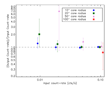
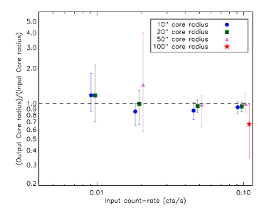
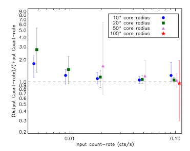
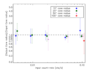
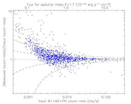
Our simulations demonstrate that the mean photometry of extended sources with Xamin is satisfactory in both pointings with or without point sources: it is unbiased for bright sources with a mean dispersion of about 20% (see fig. 4), while unavoidable the Eddington bias and scatter increase appear for fainter ones. Count rates seem somewhat overestimated only for very faint or very extended sources. The scatter increases slowly as count rates decrease but also with increasing radius.

Even when the clusters are injected into real pointings, the performances remain correct up to 50″core radius. Knowing that, for a physical core radius of $180h_{70}^{-1}$ kpc, the apparent core radii span the range $55\arcsec-22\arcsec$ for $0.2<z<1$ in $\Lambda$CDM, the goals of the pipeline are fully met. For very faint sources ($5\times 10^{-3}$ cts s^-1), the rates are somewhat underestimated, which can be explained by the fact that only the central brightest part of the sources clearly emerges from the background fluctuations. Above 50″core radii, the rates are somewhat overestimated. In addition, we notice surprisingly a weak increase of the detection efficiency of these sources when adding AGNs. The simplest interpretation is that part of the very extended sources found their emission contaminated by faint AGNs (that fall below our detection or deblending capacity), and thus tend to pass more easily the detection criteria of the pipeline, but with erroneous photometry and core radius.

A second point to note comparing the left and right panels of figure 4 is that the photometry seems tightly correlated with extension measure accuracy. A poor modelling of the source emission profile logically yields incorrect count rate estimates, particularly for very extended sources where the flux is extrapolated far outside of the fitting box. An inaccurate estimate of the source extensions is thus probably the reason for both the low count-rate and the high core radius photometry bias identified above.

3.2.2 Point sources

As shown in figure 7b, the point source photometric dispersion is basically comparable to the spread due to Poisson noise down to 20 cts. At the faint tail of the distribution, a strong Eddington bias appears.

Another issue regards point source confusion. We used our set of close pair simulations to test the deblending efficiency. The results are quite satisfactory: all $5\times 10^{-2}$ cts s^-1 pairs are deblended, while more than 65% of the $3\times 10^{-3}$ cts s^-1 sources are also. This success rate cannot easily be reached by first step detection procedures based on sliding cells having a minimum size of 10″. This point is not only important for point source statistics, but also for cluster detection, in order not to consider blended point sources as a single extended one.

3.3 Source classification using the simulations

Source selection and estimation of the selection function in surveys is always a complicated task and results from the necessary trade-off between sample completeness and contamination. For this purpose, we explored the Xamin output parameter space by means of our simulations in order to set well controlled extended/point-like source selection criteria, and to estimate contamination by spurious or misclassified sources.

3.3.1 Point sources

As AGNs represent more than 90% of the extragalactic X-ray sources at our sensitivity, we restrict ourselves to the estimation of the spurious detection rate based on our point source simulations. As can be seen in figure 5a, a simple threshold of 15 in the detection statistic gives the best balance between contamination and completeness: at this threshold, some 40 to 50 real point-like sources are detected in each pointing within 10’ of the FOV, for only 0.5 spurious ones.

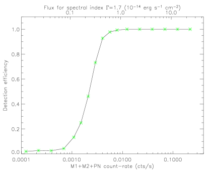
The resulting detection efficiency as a function of count rate is shown in figure 7a. The point-source flux limit (90% completeness) is about $4\times 10^{-15}$ erg s^-1 cm^-2 in [0.5-2] keV, but more than 50% of the sources are detected down to $\sim 2.5\times 10^{-15}$ erg s^-1 cm^-2.

3.3.2 Extended sources

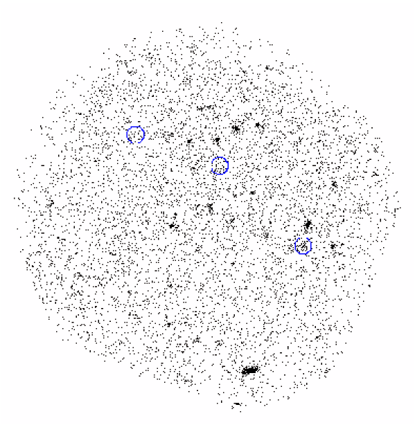
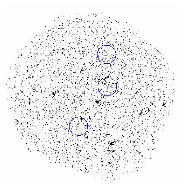
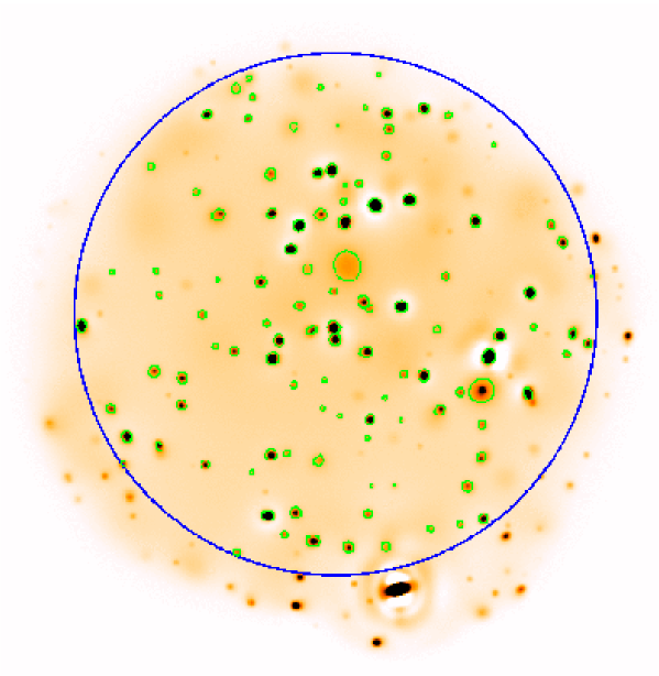
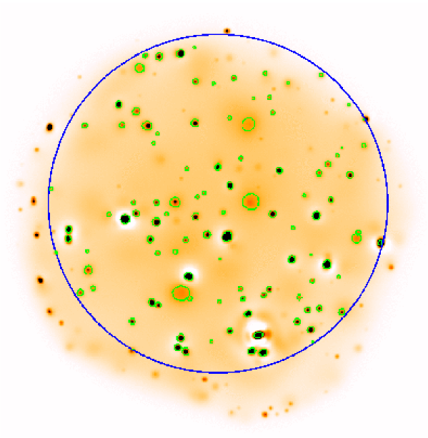
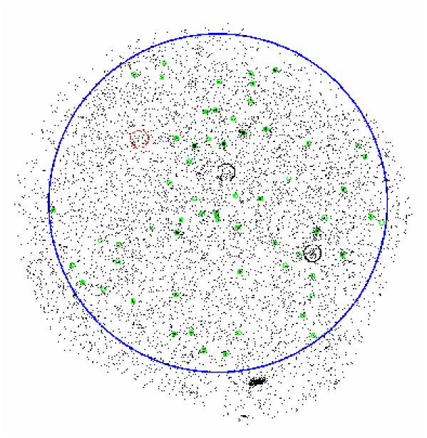
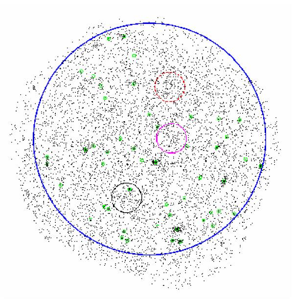
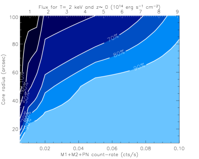
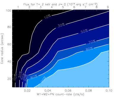
Source selection is complicated for extended sources because these objects are generally of lower surface brightness (see e.g. figure 1), and one does not only have to deal with spurious detections, but also with contaminating misclassified point sources. This task requires special care, keeping in mind the very cosmological applications of the survey. Figure 6 shows the fraction of extended sources that are detected by SExtractor in the primary catalogue as a function of flux and core radius. Our purpose is then to find a location in the Xamin output parameter space where the majority of these sources are recovered while keeping the contamination rate to a manageable level.

As a first step, we scanned the detection/extension statistic-extension space for the largest uncontaminated extended source sample. This is obtained for EXT $>$ 5″, EXT_STAT $>$ 33, and extended fit DET_STAT $>$ 32 simultaneously (see Table 2 for the definition of these parameters). From now on, we will refer to this sample as class 1 (C1) extended sources. Figure 5a illustrates the main C1 selection process in the extension $-$ extension statistic plane. .

Table 4: Source selection criteria with the XMM-LSS pipeline

Classification	Criteria
Class 1 extended	Detection statistic$>$32,
	Extension statistic$>$33,
	Extension$>$5″
Class 2 extended	Extension statistic$>$15,
	Extension$>$5″
Point source	Neither C1 nor C2,
	Detection statistic$>$15

Due to our non-contamination requirement, the C1 sample naturally excludes a number of extended sources (generally very low surface brightness or more compact sources). A less conservative sample (required by the XMM-LSS cluster search in order to detect as many valid sources as possible) can be obtained by relaxing the previous criteria to EXT $>$ 5″, EXT_STAT $>$ 15 and no DET_STAT constraint (see figure 5). From the number of detections matching these criteria in our point source simulations, we can estimate that this class 2 sample (C2) contains less than one spurious detection or misclassified point source every three pointings.

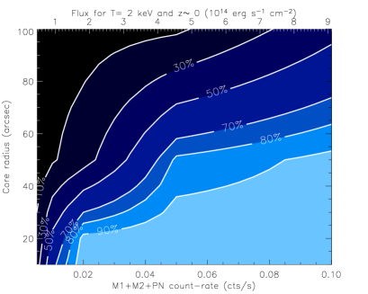
The mean detection probabilities of extended sources within 10′ of the FOV are presented for both C1 and C2 samples in figure 8, as a function of count rate and apparent core radius. As expected, this probability is higher within the C2 sample for low surface brightness and faint compact sources.

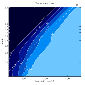
Note that detection efficiency is not a simple function of source flux as is sometimes assumed in X-ray cluster surveys (see e.g. Rosati et al. 1998), but it varies significantly when considering different source sizes, and this should be modelled to interpret correctly the results of the XMM-LSS. This impact of source extent on our detection capacity is illustrated by figure 10, where the detection probability as a function of luminosity and redshift is shown for the C2 sample, assuming a canonical core radius of $180h_{70}^{-1}$ kpc. At high redshift, where the angular distance is almost constant, our selection process closely resembles a flux limit, while the sensitivity drops at lower redshift. In this model, we find that roughly 90% of the sources down to 3 keV are detected in C2 at $z$=0.5. This number falls to 50% at a redshift of 0.9-1. A cluster similar to Coma ($\sim$8 keV) would always be detected at least as C2 up to a redshift of 1, and have more than 75% probability of being detected at $z$=2.

Table 5: Contamination statistics predicted from the simulations for each XMM-LSS pipeline source sample

Real source type	Classification	$N_{Src}$/pointing
Point-like	class 1	0.0
Point-like	class 2	0.17
Spurious	class 1	0.0
Spurious	class 2	0.10
Spurious	point-like	0.53

3.4 Validation on real data

To further validate our selection criteria, we processed all available XMM-LSS pointings and compared the pipeline output with our simulation results. Our X-ray data currently consist of 51 XMM-NEWTON pointings; 19 of them (G pointings) were obtained from guaranteed-time observation as part of a joint Liège/Milan/Saclay program (XMDS, Chiappetti et al. 2005) and have $2\times 10^{4}$ s exposure; the remaining 32 are $10^{4}$ s long and were obtained with guest-observer time. Among these, three pointings (one G and two B) are unusable due to very high background levels (probable solar flare contamination).

3.4.1 Point sources

In our 30 $10^{4}$ s exposure pointings, we obtain on average 45.8 sources per pointing with DET_STAT $>$ 15 for the point source fit. As a comparison, taking into account the detection probabilities of figure 7 and integrating over the $\log(N)-\log(S)$ of Moretti et al. (2003) between $5\times 10^{-16}$ and $1\times 10^{-11}$ erg s^-1 cm^-2 yields on average 47.4 sources per pointing. Though the matching is already satisfactory, the remaining difference mostly reflects the lack of very bright sources in the XMM-LSS area (probably due to cosmic variance) identified by Gandhi et al. (2006).

We additionally cross-identified our sources with those of the XMDS/VVDS $4\sigma$ catalogue (Chiappetti et al., 2005) which results from an alternate analysis of the G fields (that mainly uses the standard XMM-SAS procedures and is thus suitable only for point sources). We found a very good agreement with both detected sources and their characteristics. Xamin count rates are always within the error bars of XMM-SAS emldetect measurements for sources that do not fall on CCD gaps. Moreover, our detection statistic values are tightly correlated to their detection probability estimates.

3.4.2 Extended sources

Until now, the XMM-LSS optical spectroscopy follow-up program (see Pierre et al. 2004) enabled us to confirm about 60 cluster candidates. This allowed cross-checking the definition of our selection criteria obtained from the simulations against real data.

As regards the C1 sample, only genuine extended X-ray sources are detected, as expected, with no additional contamination. The majority ($\approx$85%) of the extended C1 sources are clusters, the remainder being nearby galaxies. A little contamination, around 0.5 false detections per pointing, is observed in the C2 sample (in the present datasets, this amounts to about 50% of the newly-detected sources, once the nearby galaxies and C1 clusters have been excluded). This false detection rate, while still acceptable for a survey with optical follow-up, is slightly higher than our estimates from simulations, and this is probably the result of neglecting the AGN correlation function (thus lowering the number of non-deblended close pairs of AGNs). Another possibility is that we are detecting some AGNs that are included in cosmological filaments with weak X-ray emission, which was not accounted for in the simulations.

3.4.3 Example runs on z$>$1 clusters

We ran the pipeline on the archival XMM-NEWTON observation 0111790101, for which detection of the highest redshift X-ray cluster to date, XMMUJ2235.3-2557, at $z\sim 1.4$ was reported (Mullis et al., 2005). The observation was performed in the MEDIUM FILTER and EPIC-PN small window mode so that the source, located 7.7′ from the optical axis, is only observed in the EPIC-MOS detectors. Using the full $4.5\times 10^{4}$ s exposure of the pointing ($\approx$ $3\times 10^{4}$ s at the source position), the cluster is easily identified as a C1 extended source. We further simulated the XMM-LSS observing conditions by analyzing only the first $10^{4}$ s of the observation. XMMUJ2235.3-2557 is still detected with extended fit DET_STAT=93.8, EXT_STAT=31.1 and EXT=9.8, as a C2 extended source, at the limit of the C1 parameter space, and would therefore have been detected as C1 in the exact XMM-LSS observing conditions (i.e. using THIN FILTER and with EPIC-PN data available). The ease with which this high redshift cluster is detected is mainly due to its apparent brightness: $\sim$ 220 (resp. 70) photons were available in the $4.5\times 10^{4}$ s ($10^{4}$ s) exposure. For comparison, we note that the z=1.22 cluster XLSSJ022302.6-043621 detected by Bremer et al. (2006) in the XMM-LSS survey is classified as a C2 source (EXT=5.4, EXT_STAT=15.4, and DET_STAT=51.4) with only 58 photons available for the fit.

4 The XMM-LSS selection function

Our simulation programs provide us with tools to compute the XMM-LSS selection function. We can derive the detection probability as a function of source characteristic for any exposure time, background level, and position on the detector.

Figure 7 shows the point-source detection probability inside a radius of 10′ from the mean optical axis as a function of flux. From this, a direct estimate of our mean sky coverage can be obtained.

For a given cosmology, a galaxy cluster of given luminosity, temperature, physical extent and redshift can be described by an angular core radius and a detected XMM count rate, for which figure 8 gives the detection probability for C1 and C2. We are therefore now able to properly describe our galaxy cluster selection process.

As an illustration, we compute below the expected redshift distribution of C1 and C2 clusters in $\Lambda$CDM cosmology.

4.1 Cosmological model

In the following, the cosmological parameters that determine the dynamics and content of the universe are set to WMAP values (Spergel et al., 2003) namely:
$H_{0}=71$ km s^-1 Mpc^-1, $\Omega_{m}=0.27$, $\Omega_{\Lambda}=0.73$, $\Omega_{b}=0.044$, $n=0.93$ and $\sigma_{8}=0.84$.

4.1.1 Mass function

The shape of the linear power spectrum $P(k)$ is computed at z=0 using the initial power law dependency in $k^{n}$ and the transfer function from Bardeen et al. (1986). The influence of baryons on the transfer function was modelled using the shape parameter:

$$\Gamma=\Omega_{m}h\times exp\left[-\Omega_{b}\left(1+\sqrt{2h}/\Omega_{m}\right)\right]$$ (8)

introduced by Sugiyama (1995), and the overall spectrum is normalized to $\sigma_{8}$.

Then at each redshift value on a fine grid: $P(k)$ is evaluated from its z=0 value using the linear growth factor from Carroll et al. (1992) and $\sigma(M)$ is deduced. The comoving halo number density as a function of mass, $dn/dm(z)$, is computed using the Sheth & Tormen (1999) mass function.

This common procedure to determine the halo mass function has been largely tested on numerical simulations and is known to provide accurate predictions as long as one defines the mass of the haloes to be the one included inside $r_{200b}$, the radius that encloses an overdensity of 200 with respect to the mean background density.

4.1.2 Applying the selection function

Knowledge of the cluster scaling relations is needed to predict the temperature and luminosity of these haloes and compute XMM count rates. Unfortunately, one generally doesn’t have access to the mass in $r_{200b}$ from the X-ray data, and a halo profile model is required in order to convert the mass function to another mass definition.

For this purpose, we used NFW profiles with scaling radius $r_{s}$ provided by the model of Bullock et al. (2001) which relates $r_{s}$ to the virial mass of the halo through the concentration parameter $c=r_{vir}/r_{s}$. The conversion itself is performed using the formulae provided by the appendix of Hu & Kravtsov (2003).

The emission-weighted gas temperature is derived using the local $M_{200}$-$T$ relation of Arnaud, Pointecouteau & Pratt (2005), i.e. a slope of $\alpha=1.49$, valid for clusters with $T>4$ keV. At lower temperatures, we added a gradual steepening of the correlation ($\alpha=1.85$ below 4 keV and $\alpha=2$ below 2 keV) as indicated by several recent works (see e.g. Finoguenov et al. 2001). No evolution of the $M_{200}$-$T$ relation with redshift was supposed. As an arbitrary condition to be considered as a group or cluster, we subsequently removed all haloes with $T<1$ keV.

Bolometric luminosities are then computed using the $L_{X}$-$T$ relation of Arnaud & Evrard (1999) with no evolution. Though there is some evidence that the local $L_{X}$-$T$ relation also steepens at low $T$, this seems to be important only for $T\leq 1$ keV (Ponman et al., in preparation) and is consequently ignored.

The total XMM-NEWTON EPIC count rate is estimated using an APEC thermal plasma emission model (Smith et al, 2001) with neutral hydrogen absorption as modelled by Morrison & McCammon (1983) using fixed column density of $2.6\ 10^{20}$ cm^-2 (representative of our field) folded through the EPIC response matrices for the THIN filter in accordance with our observing mode.

The selection function is finally applied assuming a constant physical core radius of $180h_{70}^{-1}$ kpc.

4.2 Results

Using this simplified model and the selection functions obtained from the simulations, we find that:

• The C2 sample should contain roughly 12 clusters per deg². When the XMM-LSS is complete, it will thus constitute the deepest X-ray selected galaxy cluster sample over a wide area.

• The C1 sample should contain some 7 clusters per deg². While this source density is a bit lower than for C2, this selection process can be applied to the whole of the XMM archive, regardless of expensive and time consuming optical spectroscopy follow-up, as the sample is effectively uncontaminated.

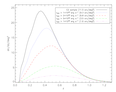
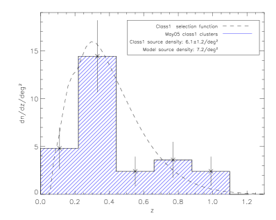
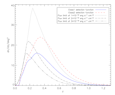
The expected redshift distribution for both samples is shown in figure 9. Panel (a) of that same figure also gives an idea of the luminosity distribution of the C2 sample.

To validate these results, we compared them with the redshift distribution of the observed C1 clusters. The sample contains 29 sources of which 24 have already been spectroscopically confirmed. Assuming that the 5 missing sources ($\sim$ 17% of the sample) will not alter significantly the current distribution, we find very good overall agreement with our prediction (fig. 9b).

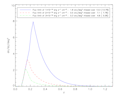
A further interesting result, already outlined in section 3.3.2 and fig. 8, is that our selection process doesn’t reproduce a flux limited sample, especially at $z<0.6$ where the change in angular distance is significant (see figure 11a).

This point is further illustrated in fig. 11b where we investigate our detection efficiency as a function of cluster flux. This shows, for the assumed cluster population, the a priori impossibility of constructing a flux limited sample from our primary catalogues, even accepting a substantial contamination level, unless a very high flux limit is set. In the present study, SExtractor is run on optimally filtered images (retaining only significant structures above $3\sigma$) with a very sensitive detection threshold and our results suggest that we have reached the limit of the data. This therefore challenges any further attempt aiming at defining deep flux limited samples with XMM.

4.3 Limitations of the present model

Although the matching between this simple model and our data (as shown in fig. 9b) is impressive, one should keep in mind that some ingredients of the model are still uncertain (and this is precisely the purpose of the XMM-LSS to try to constrain them).

In particular, while the evolution of the $M_{200}$-$T$ relation is still unknown, there seems to be indication of a positive evolution as predicted by self-similar models (see e.g. Ettori et al. 2004, Maughan et al. 2005). However none of these studies is probing our range of temperature and redshift, and the influence of non-gravitational processes can well alter this behaviour in the group regime, thus the use of the simplest non-evolving relations.

Also, in order to properly take into account the varying gas distribution with cluster mass, our assumption of a fixed core radius may seem too simple and one would have to consider lower $\beta$ values for the groups as indicated by observations (e.g. Osmond & Ponman 2004). However such data are generally largely dominated by scatter and there is currently no well-established scaling relation for these global trends.

Finally, a large fraction of the observed scatter on all these scaling relations is intrinsic to the source properties and results from the complex process of hierarchical merging in cold dark matter cosmologies and feedback from non-gravitational activity.

These are a number of caveats that neeed to be taken into account in the interpretation of such a small sample of low temperature systems. In a forthcoming paper (Pacaud et al., 2006), where we will present the full cluster catalogue, we shall further discuss the effect of the various cluster scaling laws and evolution schemes on the $dn/dz$ using as input our $L-T$ relation for groups at redshift around 0.5.

5 Summary and conclusions

We have described the procedure that we developed to analyse the $1\times 10^{4}-2\times 10^{4}$ s XMM images of the XMM-LSS survey. The main motivation of this work is the need for assembling a sample of clusters of galaxies out to a redshift of unity with controlled selection effects, suitable for cosmological and evolutionary studies. The resulting pipeline consequently combines multi-resolution wavelet filtering (MR1) to reach the source detection limit, with a subsequent maximum likelihood analysis (Xamin) to characterize the source properties.

The performances of the adopted procedure have been duly tested by means of extensive image simulations: either reproducing all instrumental and astrophysical effects, or injecting extended and point-like sources into already existing pointings. This allowed us to investigate the ultimate capabilities such as: resolving power, cluster detectability and characterization as a function of flux and apparent size, photometric accuracy. In this respect, our package constitutes a significant improvement over the standard SAS and the XMDS procedure (Chiappetti et al., 2005), specially for the extended source analysis.

Moreover, the Xamin output parameter space, densely scanned by the simulations, provides a powerful means to interpret the detected sources. In this way, we are able to define two classes of extended sources: the C1 class which is basically uncontaminated by misclassified point-like sources, and the C2 class allowing for some 50% contamination. This selection process, derived from the simulations, has been subsequently checked and validated against the current XMM-LSS sample of spectroscopically confirmed galaxy clusters.

Finally, considering a canonical power spectrum combined with a simple halo model providing $n(M,z)$ and simple cluster scaling laws ($M$-$T$-$L$) in a $\Lambda$CDM cosmology allowed us to predict the $dn/dz$ distribution of the C1 cluster population. Comparison with our current C1 data sample shows a very good agreement. From this, we infer that our goal of producing a cluster sample with controlled selection effects is fulfilled at this stage. An important point to be further emphasized is that the resulting sample is not flux limited - a concept that is anyway not rigorously applicable when dealing with extended sources spanning a wide range in flux and size.

The way the C1 class is defined allows us to construct a purely X-ray selected cluster sample with a high number density of $\sim 7$/deg² in the redshift range [0-1.2]. Moreover, an unprecedented density of $\sim 12$/deg² can be obtained with the C2 sample which includes objects down to a flux of $\sim~{}5\times 10^{-15}$ erg s^-1 cm^-2. This opens the door to the routine construction of unbiased cluster samples from XMM images.

In the very near future, with the compilation of the full XMM-LSS cluster sample over the currently existing 5 deg², we shall refine the cosmological modelling of the observed $dn/dz$ (Pacaud et al., 2006). In particular, we shall further investigate the effect of varied evolution schemes of the scaling relation, and assumptions on cluster sizes and shapes (including scatter on these average trends). Both aspects are especially relevant for the $T<$ 2 keV groups out to $z\sim$ 0.5, a population that the XMM-LSS is for the first time unveiling and that constitute the bulk of our sample. Noting that the C1 cluster sample is almost identical to the sample for which we can measure a temperature (Pierre et al., 2005), we shall also be in a position to constrain the evolution of the $L_{X}$-$T$ relation.

The combined $dn/dz$, $L_{X}$-$T$, and shape-modelling will provide very useful constrains on numerical simulations, the missing link between the theoretical parameter $M$ and the observable $L_{X}$, and consequently a self-consistent description of the building blocks of the present day clusters.

Figure 1: Examples of simulated $10^{4}$ s XMM-NEWTON images (co-addition of the EPIC cameras). Both contain point sources distributed following the X-ray Log(N)-Log(S). Blue circles show the position of simulated clusters. Top: clusters have core radii of 20″and on-axis count rates of (from top to bottom) 0.02, 0.01 and 0.03 cts s^-1. Bottom: clusters have core radii of 50″and on-axis count rates of (from top to bottom) 0.03, 0.02 and 0.05 cts s^-1. Displayed clusters are very faint (close to the detection limit) so as to illustrate the detection capabilities of the pipeline.

Figure 2: Wavelet images of fig. 1 simulations, overlayed with SExtractor catalogues. The blue circle shows the central 13′ radius of the FOV (centered on the mean optical axis) where SExtractor detections are performed.

Figure 3: Raw images of fig. 1 simulations, overlayed with Xamin catalogues. The green 10″ radius circles show the detected point sources (see fig. 4 for the selection criteria); black and magenta circles show the C1 and C2 clusters respectively. Clusters not flagged by Xamin as C1 or C2 are indicated by red dashed-line circles.

Figure 4: Extended source characterisation with the XMM-LSS pipeline within 10′ of the FOV for $10^{4}$ s exposures. For all plots, vertical bars show the standard deviation of measured points. Upper plots show the results for clusters in pointings without point sources, lower plots show the results when clusters are injected into real pointings. Left: photometry as a function of on-axis counts and core radius. Right: source extension measure as a function of on-axis counts and core radius. In all the plots, only the bins encompassing at least 10 recovered sources are shown.

Figure 5: Determination of the XMM-LSS pipeline selection criteria. AGNs are displayed as green diamonds, galaxy clusters as blue squares. Red triangles stand for spurious detections. Panel (a): Selection of point sources in the Count Rate - Detection Likelihood plane; the solid line at Likelihood=15 defines the point source sample. Panel (b): cluster selection in the Extent - Extension Likelihood plane; the solid lines at Extent=5″  and Likelihood=15 define the C2 sample; the dashed line shows the extension likelihood criteria of the C1 sample.

Figure 6: Detection probability for extended sources by SExtractor; this can be considered as the ultimate sensitivity with $10^{4}$ s XMM images, but the contamination is maximal.

Figure 7: Point source analysis with the XMM-LSS pipeline within 10′ of the FOV for $10^{4}$ s exposures. Panel (a): detection probability as a function of count rate. Panel (b): photometry, dashed and dotted-dashed lines show respectively the intrinsic $1\sigma$ and $3\sigma$ scatter expected from Poisson noise.

Figure 8: Extended source detection efficiency of the XMM-LSS pipeline in $10^{4}$ s exposures as a function of source counts and core radius inside 10′  of the FOV. Panel (a): C1 sample. Panel (b): C2 sample.

Figure 9: Cosmological expectations of the C1 and C2 samples for sources with $T>$ 1 keV. Panel (a): Luminosity and redshift distribution of the C2 sample. Panel (b): redshift distribution of the observed C1 sources (29 sources, 24 with redshifts) compared to the $\Lambda$CDM expectations.

Figure 10: Probability of detecting a cluster located inside the central 10′  of the FOV as a C2 source as a function of its redshift and luminosity given our cosmological model within $10^{4}$s pointings. An indicative flux limit of $2\times 10^{-14}$ erg.s^-1.cm^-2 is shown by the thick dashed line.

Figure 11: Comparison of our source selection process with the common assumption of a flux limited sample for sources with $T>$ 1 keV. Panel (a): expected $dn/dz$ for class 1 (blue) and class 2 (red) compared to flux limited surveys; on average, we detect higher redshift clusters than flux limited surveys with the same source density. Panel (b): redshift distribution of the sources not detected by the first pass (MR/1 + SExtractor) above several flux limits, assuming the source population generated by our simple cosmological model (we miss the low end of the luminosity function).

References

- Arnaud & Evrard (1999) Arnaud, M., & Evrard, A. E. 1999, MNRAS, 305, 631
- Arnaud, Pointecouteau & Pratt (2005) Arnaud, M., Pointecouteau, E., & Pratt, G. W. 2005, A&A, 441, 893
- Bardeen et al. (1986) Bardeen, J. M., Bond, J. R., Kaiser, N., & Szalay, A. S. 1986, ApJ, 304, 15
- Bertin & Arnouts (1996) Bertin, E., & Arnouts, S. 1996, A&AS, 117, 393 (SExtractor)
- Bremer et al. (2006) Bremer, M. N., Valtchanov, I., Willis, J., et al. (2006), submitted to MNRAS
- Bullock et al. (2001) Bullock, J. S., Kolatt, T. S., Sigad, Y., Somerville, R. S., Kravtsov, A. V., Klypin, A. A., Primack, J. R., & Dekel, A. 2001, MNRAS, 321, 559
- Cash (1979) Cash, W. 1979, ApJ, 228, 939
- Carroll et al. (1992) Carroll, S. M., Press, W. H., & Turner, E. L. 1992, ARA&A, 30, 499
- Cavaliere & Fusco-Femiano (1976) Cavaliere, A., & Fusco-Femiano, R. 1976, A&A, 49, 137
- Chiappetti et al. (2005) Chiappetti, L., Tajer, M., Trinchieri, G. et al. 2005, A&A, 439, 413
- Eke, Navarro & Steinmetz (2001) Eke, V. R., Navarro, J. F., & Steinmetz, M. 2001, ApJ, 554, 114
- Ettori et al. (2004) Ettori, S., Tozzi, P., Borgani, S., & Rosati, P. 2004, A&A, 417, 13
- Finoguenov et al. (2001) Finoguenov, A., Reiprich, T. H., & Böhringer, H. 2001, A&A, 368, 749
- Gandhi et al. (2006) Gandhi, P., Garcet, O., Disseau, L. et al. 2006, A&A in press
- Hu & Kravtsov (2003) Hu, W., & Kravtsov, A. V. 2003, ApJ, 584, 702
- Infante (1987) Infante, L. 1987, A&A, 183, 177
- Kron (1980) Kron, R.G. 1980, ApJS, 43, 305
- Maughan et al. (2005) Maughan, B. J., Jones, L. R., Ebeling, H., & Scharf, C. 2006, MNRAS, 365, 509
- Moretti et al. (2003) Moretti, A., Campana, S., Lazzati, D., & Tagliaferri, G. 2003, ApJ, 588, 696
- Morrison & McCammon (1983) Morrison, R., & McCammon, D. 1983, ApJ, 270, 119
- Mullis et al. (2005) Mullis, C. R., Rosati, P., Lamer, G., Böhringer, H., Schwope, A., Schuecker, P., & Fassbender, R. 2005, ApJL, 623, L85
- Osmond & Ponman (2004) Osmond, J. P. F., & Ponman, T. J. 2004, MNRAS, 350, 1511
- Pierre et al. (2004) Pierre, M., Valtchanov, I., Altieri, B. et al. 2004, JCAP, 9, 11
- Pierre et al. (2005) Pierre, M., Pacaud, F., Duc, P.-A. et al. 2006, MNRAS in press
- Pacaud et al. (2006) Pacaud, F. et al. 2006, in preparation
- Pratt & Arnaud (2002) Pratt, G., & Arnaud, M. 2002, A&A, 394, 375
- Press et al. (1992) Press, W. H., Teukolsky, S. A., Vetterling, W. T., & Flannery, B. P. 1992, Cambridge: University Press, 2nd ed.
- Read & Ponman (2003) Read, A. M., & Ponman, T. J. 2003, A&A, 409, 395
- Rosati et al. (1998) Rosati, P., della Ceca, R., Norman, C., & Giacconi, R. 1998, ApJL, 492, L21
- Spergel et al. (2003) Spergel, D. N., Verde, L., Peiris, H. V. et al. 2003, ApJS, 148, 175
- Sheth & Tormen (1999) Sheth, R. K., & Tormen, G. 1999, MNRAS, 308, 119
- Smith et al (2001) Smith, R. K., Brickhouse, N. S., Liedahl, D. A., & Raymond, J. C. 2001, ApJL, 556, L91 (APEC)
- Starck et al. (1998) Starck, J.-L., Murtagh, F., & Bijaoui, A. 1998, Image Processing and Data Analysis: The Multiscale Approach (Cambridge Univ. Press) (UK) (MR/1)
- Starck & Pierre, (1998) Starck, J.-L., & Pierre, M. 1998, A&AS, 128, 397
- Sugiyama (1995) Sugiyama, N. 1995, ApJS, 100, 281
- Valtchanov et al. (2001) Valtchanov, I., Pierre, M., & Gastaud, R. 2001, A&A, 370, 689
- Vikhlinin et al. (1998) Vikhlinin, A., McNamara, B. R., Forman, W., Jones, C., Quintana, H., & Hornstrup, A. 1998, ApJ, 502, 558