Is there a caustic crossing in the lensed quasar Q2237$+$0305 observational data record?

Abstract

We re–investigate the gravitationally lensed system Q2237$+$0305 data record to quantify the probability of having a caustic crossing in the A component. Several works assume that this is the case, but no quantitative analysis is available in the literature. We combine the datasets from the OGLE and GLITP collaborations to accurately trace the prominent event in the lightcurve for the A component of the system. Then the observed event is compared with synthetic light curves derived from trajectories in magnification maps. These maps are generated using a ray–tracing technique. We take more than 10⁹ trajectories and test a wide range of different physical properties of the lensing galaxy and the source quasar (lens transverse velocity, microlens mass, source intensity profile and source size). We found that around 75% of our good trajectories (i.e. that are consistent with the observations) are caustic crossings. In addition, a high transverse velocity exceeding 300 km s^-1, a microlens mass of about 0.1 M_⊙ and a small standard accretion disk is the best parameter combination. The results justify the interpretation of the OGLE–GLITP event in Q2237+0305A as a caustic crossing. Moreover, the physical properties of the lens and source are in very good agreement with previous works. We also remark that a standard accretion disk is prefered to those simpler approaches, and that the former should be used in subsequent simulations.

1 Introduction

The system QSO 2237$+$0305 is formed by a distant source quasar at $z_{Q}=1.695$ and a spiral lens galaxy at $z_{G}=0.039$ that quadruples the images of the source (Huchra et al. 1985). Nowadays, it is one of the best studied gravitationally lensed quasar systems which has been monitored by a number of groups in the last years (Corrigan et al. 1991, Østensen et al. 1996, Vakulkik et al. 1997, Woźniak et al. 2000, Alcalde et al. 2002, Schmidt et al. 2002). Among these monitoring campaigns, two of them have produced excelent light curves: OGLE (Woźniak et al. 2000) and GLITP (Alcalde et al. 2002). The former collaboration covers a time frame of several years, while the latter a few months but with a daily sampling, bad weather or technical problems aside. Interestingly, the two datasets overlap each other during a period of time.

The recent datasets have been used to investigate several physical properties of the system. Limits on the size of the quasar emission region and the mass of the central black hole have been placed by Wyithe et al. (2000a), Yonehara (2001), Shalyapin et al. (2002), Goicoechea et al. (2003) and Kochanek (2004); the mass range of the microlenses in the lensing galaxy has been established by Wyithe et al. (2000b) and Kochanek (2004); and limits on the transverse velocity of the lensing galaxy have been reported by Wyithe et al. (1999) and Gil–Merino et al. (2005). To explain the prominent OGLE–GLITP event in the brightest component (A), some of these authors have assumed a caustic crossing (e.g., Goicoechea et al. 2003, Moreau et al. 2005). This interpretation of the OGLE–GLITP event in the A component (caustic crossing) is supported by the best trajectories in terms of $\chi^{2}$ that appear in Kochanek (2004). Although Kochanek (2004) also showed other relatively good trajectories passing through complex magnification regions, the caustic crossing scenario became popular for studying the nature of the source quasar, e.g., reconstruction of the intrinsic brightness profile or estimation of the size ratios (Bogdanov & Cherepashchuk 2004, Goicoechea et al. 2004, Koptelova & Shimanovskaya 2005).

In this contribution we merge the available data of the prominent OGLE–GLITP event (it was monitorized by both OGLE and GLITP collaborations), building a single dataset for the A component. We try to find the probability of having a caustic crossing in this component considering different source profiles and sizes, microlenses masses and lens transverse velocities. In this way we both justify those works that assumed approximations to caustic crossings and future assumptions.

The paper is organised as follows: Sec. 2 describes the way in which the datasets from the different OGLE and GLITP collaborations are merged to produce a single set; Sec. 3 explains the method used to produce the synthetic light curves; Sec 4 establishes the criteria to compare the synthetic light curves and the observational record, and gives the results of these comparisons; finally, in Sec. 5 we include our conclusions.

2 Data Merging

We are interested in the A component of Q2237$+$0305. The system was monitored by the phase II of the OGLE project. During part of that period, the GLITP project obtained optical frames of the same lens system. In particular, the overlapping period was approximately between the Julian days 2451400–2451600, corresponding to from October 1999 until February 2000. The corresponding observational data set from both campaings in the $V$ filter is displayed in Fig. 1. From now on we use a simpler scale of time: JD–2450000, so a peak of flux around day 1500 is seen in Fig. 1.

Figure 1: $V$-band photometry of the A component of Q2237$+$0305 for both data sets, OGLE (open circles) and GLITP (filled circles). There is still no calibration between the two sets.

In order to merge the OGLE and GLITP data sets, the first problem we found was the night sampling. During the OGLE campaign, two data points were consecutively obtained every night. The initial step is thus to “re–reduce” these data points to get one per observational day. In this way, when two points are available for a given night, the observational date and flux will be the mean of the individual observational dates and fluxes. The estimation of the errors for the new points has two cases: if the individual error bars overlap, the error is the mean of the individual errors; if they do not overlap, then the error is estimated by the square root of the sum of the square of the average of the individual errors plus the square of the difference between the mean flux and one of the two individual fluxes.

Once we have the same night sampling for both data sets, the next step is to merge them. To do that, we try to find a linear expression that relates the data sets:

$$F_{OGLE}(t)=a+b\cdot F_{GLITP}(t)$$ (1)

where $F(t)$ are the fluxes and $a$ and $b$ are the constants to be determined. We treat the problem as a $\chi^{2}$ minimization (e.g., Ofek & Maoz 2003, Bogdanov & Cherepashchuk 2004). The best fit found is

$$F_{OGLE}(t)=-0.097+1.183\cdot F_{GLITP}(t)$$ (2)

In the GLITP photometric system, the “new” OGLE data points are then

$$F^{\prime}_{OGLE}(t)=0.082+0.845\cdot F_{OGLE}(t)$$

$$\sigma^{\prime}_{OGLE}=0.845\cdot\sigma_{OGLE}$$ (3)

The resulting lightcurve is presented in Fig. 2. This is the dataset we will compare to simulations.

Figure 2: OGLE (open circles) and GLITP (filled circles) data sets have been merged following a “re–reduction” of the original OGLE data and expressions in Equation 3 (see text for further details).

3 Simulations

Prior to produce synthetic light curves, we first build magnification maps where these will be drawn. The 2–dimensional magnification maps are done using a ray tracing method: light rays are back-traced from the observer to the source plane through a distribution of mass sitting on the lens plane (Kayser et al. 1986, Wambsganss 1990). The distribution of mass responds to a macromodel of the system, that gives the two relevant parameters: the convergence $\kappa$ or the distribution of mass in compact objects at the position of the beam and the shear $\gamma$ or the influence of matter outside the beam. In general, lightcurves of lensed quasars might contain both microlensing and instrinsic variability. So in order to analyse microlensing alone one should correct for the time delay and then subtract to components. However, in the case of Q2237 the time delay is expected to be of a few hours (Vakulik et al. 2006). In addition, in the case of the period analysed here for Q2237, the flatness of component D indicates that intrinsic variability does not contribute significantly to the behavior of the components (see Shalyapin et al. 2002). We use the parameters for the A component given by Schmidt et al (1998): $\kappa=0.36$ and $\gamma=0.40$ (we note that in Gil-Merino et al. 2005 slightly different models where indistinguishable, driving to the same conclusions). The resulting density of rays at a point in the source plane is proportional to the microlensing magnification of the source at that position. The space scale factor is the Einstein radius, defined in the source plane as

$$r_{E}=\left(\frac{4GM_{\rm\mu lens}}{c^{2}}\frac{D_{s}D_{ds}}{D_{d}}\right)^{1/2},$$ (4)

where $M_{\rm\mu lens}$ is the mass of the microlenses and $D_{i}$ are angular distances: $D_{s}$ is observer–source, $D_{d}$ observer–lens and $D_{ds}$ lens–source. Setting the space scale ($r_{E}$), the value of the microlens mass is directly related to the choice of the cosmological model. The magnification maps are then convolved with a particular intensity profile for the source, which is characterized by a typical radius. We must also assume a certain effective transverse velocity for the source (transverse displacement of the source in the source plane divided by elapsed time in the observer’s clock) $V_{t}=-(1+z_{G})^{-1}(D_{s}/D_{d})v_{t,lens}$ (see e.g. Gil–Merino et al. 2005 and references therein for the relationship between the effective transverse motions of the source and the lens). The synthetic microlensing light curves are obtained extracting linear trajectories across the magnification patterns, since once all physical parameters are fixed and knowing the observational baseline of 200 days, we can calculate the length of these trajectrories. We note here that we do not take into account the additional effect of the proper motion of the microlenses. This effect would play a significant role in large time-scale lightcurves but in short time-scale campaigns the magnification maps can be considered static to this respect. Including the proper motion of microlenses, we would increase the number of caustic crossings in any case, so the results here are conservative.

To carry out the simulations we take $H$ = 66 km s^-1 Mpc^-1. For a given value of $r_{E}$ in Eq. (4), the microlens mass depends on the matter–energy density of the universe. We focus on both the Einstein–de Sitter model (EdSM: $\Omega_{M}$ = 1, $\Omega_{\Lambda}$ = 0) and the current concordance model (CM: $\Omega_{M}$ = 0.3, $\Omega_{\Lambda}$ = 0.7), so each cosmology leads to a different microlens mass, but the final statistics on the caustic crossings remains the same. Taking a particular value of $V_{t}$, we also have two different values of the effective transverse velocity for the lens, one corresponding to the EdSM and another associated with the CM. In Table 1 all the physical values are presented. We use a set of axisymmetric sources, including brightness distributions enhanced at the centre of the source (standard accretion disk and and Gaussian profiles) as well as a uniform brightness distribution. Their typical radii are consistent with previous studies by Wyithe et al. (2000a), Yonehara (2001), Shalyapin et al. (2002) and Kochanek (2004). Wyithe et al. (2000b) obtained that the most likely value for the microlens mass is in the range 0.01–1 M_⊙, while Kochanek (2004) used a CM and reported an interval 0.003–0.1 M_⊙. The values of $M_{\mu lens}$ in Table 1 (EdSM and CM) vary between a lower limit slightly above 0.01 M_⊙ and an upper limit slightly below 1 M_⊙, and they reasonably agree with previous work. With respect to the lens transverse velocities, Wyithe et al. (1999) claimed that $v_{t,lens}<$ 500 km s^-1 (EdSM). Moreover, using an intermediate microlens mass of 0.1 M_⊙, Gil–Merino et al. (2005) also inferred a constraint $v_{t,lens}<$ 630 km s^-1 (CM). Our values of $v_{t,lens}$ in Table 1 are basically consistent with these dynamical constraints.

intensity	source	$M_{\mu lens}$ (M⊙)	$v_{t,lens}$ (km s-1)
profile	radius (cm)	EdSM/CM	EdSM/CM
Uniform	6$\cdot$1014	0.05/0.04	100/75
Gaussian	2$\cdot$1015	0.10/0.08	300/220
Standard	6$\cdot$1015	0.6/0.5	600/445

Table 1: We tested three different intensity profiles, source radii, Einstein radii and effective transverse velocities for the source. The resulting simulations were obtained for all the possible combinations between these parameters. Here, standard profile means intensity profile of a Newtonian geometrically–thin and optically–thick accretion disk. The source radius is the typical radius of the intensity profile, so it is the radius of the quasar for a uniform disk, but is smaller than the quasar radial size (containing 95% of the total brightness) in the other cases (see Shalyapin et al. 2002). On the other hand, the values of $M_{\mu lens}$ and $v_{t,lens}$ depend on the cosmological model, and we present their values for the EdSM and CM with $H$ = 66 km s^-1 Mpc^-1 (see main text).

Taking into account that each convolution gives a different map, we have produced a total number of 108 magnification maps, 2$\times$2 $r_{E}$ on 2000 pixels a side each. Considering all possible combinations of the transverse velocities, the number of time maps (by transforming the spatial axes into time axes) is 3 times greater. The number of trajectories tested on each magnification pattern is 10⁷. The total CPU time for these simulations, excluding the generation of maps, was around 720 hours on a Pentium 4.

But could Nature be conspiring against us? It could happen that the variability detected in the A image (see Fig. 2) is in fact a cusp passing and what we see is a combination of a symmetric microlensing event due to the cusp plus a gradient originated by intrinsic variability. If this is true, that gradient should also appear in component D during the same period, because the time delays are of only the order of hours. Since this component is flat, the only explanation is that microlensing and intrinsic variability are mutually canceled in image D. Fortunately we can test this; we construct a magnification map for the D component of 4500 pixels on a side covering a physical length of 10 Einstein radii, and we then analysed the gradient of 10⁶ tracks of a length equal to the 200 days period of observations, for each combination of source size and transverse velocity. We search for gradients between a 15% and a 23%, the ranges associated with the gradient seen in the A component. We found that for the biggest source size considered in this study only 0.15% of the cases showed a gradient in that range. The percentage was slightly bigger, 1.16%, for the smallest source size. These results were obtained for transverse velocities of 600 km s^-1. Considering velocities of 300 km s^-1 the percentage was 0.5% for the smallest source size and 0.001% for the biggest one. Thus, we conclude that the possibility of a conspirancy between microlensing and intrinsic variability is extremely unlikely in this work.

4 Analysis and Results

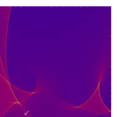
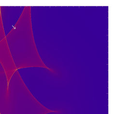
Figure 3: Caustic crossings (top and bottom panels) and cusp crossings (middle panel) that agree with the OGLE–GLITP event in Q2237+0305A (see Fig. 2). Their associated synthetic lightcurves verify Eq. 5.

Each simulated lightcurve is compared to the observational one. The way we did it is a $\chi^{2}$ test. We estimate the difference between each $\chi^{2}$ value and the the number of degrees of freedom ($\nu$), and then we select the good fits verifying

$$\delta=\frac{|\chi^{2}-\nu|}{\sqrt{2\cdot\nu}}\leqslant 1$$ (5)

where $\delta$ is the relative deviation of $\chi^{2}$ (Shalyapin et al. 2002). All the synthetic trajectories that satisfy Eq. 5 are considered as physical processes consistent with the observational lightcurve, i.e., good trajectories. Then we compute how many of them are in fact caustic crossings in their respective magnification maps. After generating a total number of 3.34$\cdot$10⁹ synthetic lightcurves, we found that 54 of them satisfied Eq. 5, with a $\langle\hat{\chi}^{2}\rangle$=1.125. Among them, 14 were not caustic crossings, but cusp crossings. This means that the event seen in the A component of Q2237+0305 can be explained as a caustic crossing in a 74% of the good trajectories generated in this contribution. The three panels of Figure 3 show some good trajectories in our magnification maps. Caustic crossings appear in the top and bottom panels of Fig. 3. However, the middle panel includes less probable (1:4) cusp crossings.

$M_{\mu lens}$ (M⊙)	trajectories with $\delta\leq 1$
EdSM/CM
0.05/0.04	26%
0.10/0.08	56%
0.6/0.5	18%

Table 2: More than a half of the good trajectories suggests a mass of the microlenses of about 0.1 M_⊙, among the values tested.

$v_{t,lens}$ (km s-1)	trajectories with $\delta\leq 1$
EdSM/CM
100/75	0%
300/220	13%
600/445	87%

Table 3: The maximum transverse velocity tested is favored by the simulations against lower values. This is interesting because the previous strongest upper limits for the effective transverse velocity were of $\sim$ 600 km s^-1.

Interestingly, the results can also be sorted attending to different criteria. For example, all the trajectories matching Eq. 5 correspond to a standard accretion disk. None of the other intensity profiles seem to be viable to explain the prominent event. Due to the size of the maps, we cannot properly test the extreme case of a standard source with the larger radius. However, considering the other two radii, the smaller one is clearly favoured (91% of the trajectories with $\delta\leq 1$). In addition, more than a half of the trajectories with $\delta\leq 1$ correspond to a microlens mass of about 0.1 M_⊙ (Table 2), and 87% of them to transverse velocities of 450–600 km s^-1 (Table 3).

5 Conclusions

Several previous works using either OGLE or GLITP (or both) data sets assumed a caustic crossing occurring in the A component of Q2237+0305 (see, e.g., Shalyapin et al. 2002). In this contribution we tested, via ray-tracing simulations, whether the event seen in component A running from October 1999 to February 2000 is compatible with a caustic crossing and to which extend. From a very large number of simulated trajectories ($>$ 10⁹) we found that only several tens were compatible with observations. These good trajectories are related to two different kinds of physical scenarios: caustic crossing (see the top and bottom panels of Fig. 3) and cusp crossing (see the middle panel of Fig. 3). A caustic crossing scenario has a probability of about 75% (40 good trajectories), whereas a cusp crossing scenario (do not confuse with a source passing close, but outwardly, to a cusp) has a smaller probability of about 25% (14 good trajectories). We checked different lens transverse velocities with an upper limit of 600 km s^-1 (Wyithe et al. 1999, Gil–Merino et al. 2005). Surprisingly, small or intermediate velocities ($\leq$ 300 km s^-1) do not seem to be the most probable ones, which means that the true transverse motion might be close to that upper limit. Our results also suggested that the mass of the microlenses at the location of image A should be very close to 0.1 M_⊙, which is in the centre of the range derived by Wyithe et al. (2000b) and is the upper limit reported by Kochanek (2004). Yonehara (2001) and Gil–Merino et al. (2005) also assumed this mass to obtain their strongest constraint on the quasar size and the lens transverse velocity, respectively. Interesting is also the fact that the best results were obtained using a standard accretion disk as intensity profile and that the smallest source size tested was the favored one. This last result is also in agreement with some previous work (Shalyapin et al. 2002, Kochanek et al. 2004). We note that we did not investigated different inclinations of the disk nor more sophisticated accretion disk models, which is an interesting issue considered as a second order effect but to be addressed in a future work. Very recently, Mortonson et al. (2005) found that the generic microlensing fluctuations are relatively insensitive to all properties of the source models except the half-light radius of the disk. Here and in other related papers it is showed the feasibility of a discrimination between different intensity profiles through the observation and analysis of caustic/cusp crossings.

References

- (1) Alcalde D., Mediavilla E., Moreau O. et al. 2002, ApJ, 572, 729
- (2) Bogdanov M.B., Cherepashchuk A.M., 2004, Astronomy Reports, 48, 261
- (3) Corrigan R.T., Irwin M.J., Arnaud J. et al. 1991, AJ, 102, 34
- (4) Gil-Merino R., Wambsganss J., Goicoechea L.J., Lewis G.F., 2005, A&A, 432, 83
- (5) Goicoechea L.J., Alcalde D., Mediavilla E., Muñoz J.A., 2003, A&A, 397, 517
- (6) Goicoechea L.J., Shalyapin V., González-Cadelo J., Oscoz A., 2004, A&A, 425, 475
- (7) Kayser R., Refsdal S., Stabell R., 1986, A&A, 166, 36
- (8) Kochanek C.S., 2004, ApJ, 605, 58
- (9) Koptelova E., Shimanovskaya E., 2005, astro–ph/0508576
- (10) Moreau O., Libbrecht C., Lee D.-W., Surdej J., 2005, A&A, 436, 479
- (11) Mortonson M.J., Schechter P.L., Wambsganss J., 2005, ApJ, 628, 594
- (12) Ofek, E. O., Maoz, D. 2003, ApJ, 594, 101
- (13) Østensen R., Refsdal S., Stabell R. et al. 1996, A&A, 309, 59
- (14) Shalyapin V.N., Goicoechea L.J., Alcalde D., Mediavilla E., Muñoz J.A., Gil-Merino R., 2002, ApJ, 579, 127
- (15) Schmidt R., Kundić T., Pen U.-L. et al. 2002, A&A, 392, 773
- (16) Schmidt R.W., Webster R.L., Lewis G.F., 1998, MNRAS, 295, 488
- (17) Vakulik V.G., Dudinov V.N., Zheleznyak A.P. et al. 1997, Astron. Nachr., 318, no.2, 73
- (18) Vakulik V., Schild R., Dudinov V., Nuritdinov S., Tsvetkova V., Burkhonov O., Akhunov T., 2006, A&A, 447, 905
- (19) Wambsganss J., 1990, PhD thesis (Munich University), also available as report MPA 550
- (20) Wyithe J.S.B., Webster R.L., Turner E.L., 1999, MNRAS, 309, 261
- (21) Wyithe J.S.B., Webster R.L., Turner E.L., 2000a, MNRAS, 318, 762
- (22) Wyithe J.S.B., Webster R.L., Turner E.L., 2000b, MNRAS, 315, 51
- (23) Woźniak P.R., Alard C., Udalski A. et al. 2000, ApJ, 529, 88
- (24) Yonehara A., 2001, ApJ, 548, L127