Variability and multi-periodic oscillations in the X-ray light curve of the classical nova V4743 Sgr

Abstract

The classical nova V4743 Sgr was observed with XMM-Newton for about 10 hours on April 4 2003, 6.5 months after optical maximum. At this time, this nova had become the brightest supersoft X-ray source ever observed. In this paper we present the results of a time series analysis performed on the X-ray light curve obtained in this observation, and in a previous shorter observation done with Chandra 16 days earlier. Intense variability, with amplitude as large as 40% of the total flux, was observed both times. Similarities can be found between the two observations in the structure of the variations. Most of the variability is well represented as a combination of oscillations at a set of discrete frequencies lower than 1.7 mHz. At least five frequencies are constant over the 16 day time interval between the two observations. We suggest that a periods in the power spectrum of both light curves at the frequency of 0.75 mHz and its first harmonic are related to the spin period of the white dwarf in the system, and that other observed frequencies are signatures of nonradial white dwarf pulsations. A possible signal with a 24000 sec period is also found in the XMM-Newton light curve: a cycle and a half are clearly identified. This period is consistent with the 24278 s periodicity discovered in the optical light curve of the source and thought to be the orbital period of the nova binary stellar system.

1 Introduction

Time series of astronomical observations are crucial for the study of variable stars in general, and of Cataclysmic Variables in particular. For Classical Novae (CN), X-ray time series give us information about temporal characteristics of very localized areas within these stellar systems that are inaccessible at other wavelengths. In particular, in a classical nova system, in the X-ray range we may be observing directly the surface of the white dwarf (WD) or the very inner region around it. This gives us a direct look into the temporal behaviors of the site where the thermonuclear outburst takes place.

In this paper we report results obtained from our analysis of X-ray light curves (LC), using data obtained with the XMM- Newton telescope for the classical nova V4743 Sgr (N Sagittarii 2002 No. 2), about 6.5 months after the nova outburst. We also reanalyze the X-ray light curve of the nova observed with Chandra two weeks earlier (see Ness et al 2003). The results we present here provide us with details of information that is hardly obtained by any other means, underlining the great potential of time series applied to X-ray observations.

2 Nova V4743 Sgr

Nova V4743 Sgr (Nova Sgr 2002 no. 2) was discovered in outburst in September of 2002 and reached V=5 on 2002 September 20 (Haseda 2002). It was a very fast nova, with a steep decline in the optical light curve and large ejection velocities. The time to decay by 3 mag in the visual (t₃), was 15 days and the Full Width at Half Maximum (FWHM) of H$\alpha$ line reached 2400 km s^-1 (Kato 2002). An estimate of the distance based on infrared observations is $\approx$6.3 Kpc (Lyke et al. 2002).

In December 2002, the nova was observed for the first time with Chandra ACIS-S. At that time the nova was a very soft and moderately luminous X-ray source, with a count rate about 0.3 cts s^-1. There were indications that the nova was not at the peak of X-ray luminosity yet, so a Chandra-LETG grating observation was done on 2003 March 20. A description of the instrument is found in Brinkman et al., (2000). The count rate was astonishingly high, 40 cts s^-1 during 3.6 hours, then a slow decay, lasting for an hour and a half, was followed by another 1.5 hours of very low luminosity with a measurement of only $\approx$0.02 cts s^-1 (Ness et al. 2003, Starrfield et al. 2003).

A decline of a supersoft X-ray source in a nova was observed once before with BeppoSAX, in V382 Vel (Orio et al. 2002). The reason for the sudden decline remains unexplained. Before the decline, the unabsorbed flux in the Chandra observation of V4743 Sgr was close to 10^-9 erg cm^-2 s^-1 and the spectrum was extremely soft, with atmospheric absorption features (Rauch et al. 2005, Petz et al. 2005). During the high luminosity and the decay phases, a periodicity of 1324 s was detected, with fluctuations of 20% of the mean count rate (see Starrfield et al. 2003, Ness et al. 2003).

Wagner et al. (2003) discovered a period of 24278$\pm$259 s in the optical light curve of the star. They proposed that this is the orbital period of the nova binary stellar system. The $\simeq$24000 sec periodicity was measured again in the optical LC of the star in July 2004 (Wagner et al, 2006). These authors found also a period of 1341 sec in that LC as well as a period of 1419 sec which seems to be a beat period of the above two.

3 A new observation with XMM-Newton

A new observation program was proposed by us to the XMM-Newton Project Scientist as a target during the Discretionary Time. The nova was observed with this telescope on April 4 2003, for 10 hours (see Orio et al. 2003). A description of the mission can be found in Jansen et al. (2001). Three X-ray telescopes with five X-ray detectors were all used: the European Photon Imaging Camera pn (see Strüder et al. 2001), two EPIC MOS cameras (Turner et al. 2001), and two Reflection Grating Spectrometers (RGS-1 and RGS-2, (see den Herder et al. 2001). The observation lasted a little over 36000 seconds with EPIC and the RGS-1 and RGS-2 overlap for 35306 seconds. The satellite carries also a UV/Optical telescope (OM; Watson et al. 2001). Observations with this instrument where carried out in imaging mode with the UVW1 filter (effective wavelength: 291 nm). 35 exposures were done with exposure times 800 s, which were too long for the timing analysis done in this article. The average count rate was 252$\pm$10 cts s^-1, and we measured an average flux 1.2 $\times 10^{-13}$ erg cm^-2 s^-1. The RGS spectra are discussed in detal in a forthcoming article (Orio et al. 2006, in preparation).

The data obtained by the two EPIC MOS cameras suffered from very severe pile up effect that made them unsuitable for our analysis. The data initially collected by the EPIC pn camera, operated in the prime mode, with the full window, and the thin filter, suffer from the same effect during the first 79 minutes of observation. The operation of the pn camera was then switched to timing mode to avoid severe pile-up. Here we use only the data obtained in timing mode, disregarding the first $\approx$5000 seconds of the EPIC-pn imaging mode observations. The measured average, background corrected count rate in timing mode was 1309.5$\pm$0.3 cts s^-1 (Orio et al. 2003). The variations are by up to 40%.

The data were reduced with the ESA XMM Science Analysis System (SAS) software, version 5.3.3., using the latest calibration files available in July of 2005. We further subdivided the EPIC-pn data into three different “supersoft” distinct energy bands: low: 0.2-0.4 keV, medium: 0.4-0.6 keV and high: $>$0.6 keV The RGS count rates are about 57 cts s^-1. The unabsorbed flux was measured by us to be 1.5 $\times$ 10^-9 erg cm^-2 s^-1, consistent with the flux measured 16 days earlier with Chandra.

4 The two X-ray Light Curves

4.1 The April 2003 XMM light curve

The XMM data reduced from the various instrument on board the satellite as described above, provided us with six X-ray LC of the source, of which five are independent of each other. These are the 2 RGS and the 3 “color” EPIC-pn LC. The 6th LC is the integrated EPIC-pn LC. The optical/UV data was not useful for the analysis presented in this paper since the exposures were 800 s long.

The data extracted from the RGS-1 and RGS-2 grating were binned into 0.574 s wide bins. This is the time it takes to read each one of the eight CCDs that together collect the photons of the whole spectrum. The RGS dispersion gratings cover the 5-35 Å wavelength range (0.35- 2.5 keV), although we obtained useful signal only in the 26-35 Å range. The RGS data are also piled-up, but in a dispersion instrument, piled-up events at a discrete wavelength increase in pulse height amplitude by an integer multiple of the intrinsic energy. Furthermore, since the softness of the source precludes any intrinsic photons from higher spectral orders, we can confidently identify events that occur within the higher order spectral masks for an on-axis point source as piled-up first order photons. This is verified by line matching of the piled-up events using the first order response matrix. Source events dominate over background and scattered source light in the first three orders. Consequently we added events within the second and third order extraction masks to the first order events, thus reclaiming the piled-up events and increasing the signal-to-noise of the spectra.

The LC of the EPIC-pn camera in timing mode cover the last 30000 seconds of the two RGS light curves. The time resolution of EPIC- pn in this mode is 0.03 msec, but the light curve turned out to have many short (few seconds) time intervals excluded from the Good Time Intervals (GTI), mainly because the source count rate was too high for the available telemetry band width, and as a result part of the data were lost. The measured pn light curve is thus split into many portions lasting a few seconds each, with “holes” of few seconds duration in the light curve. The energy range of the pn camera is 0.2-10 keV, and the light curve we present and discuss in this paper was extracted with 1 second wide time bins. The broad band pn data were subdivided into the three narrow band light curves described above : LOW, MED, and HIGH.

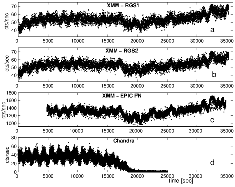
Figure 1: X-ray light curves of V4743Sgr: (a) XMM-Newton RGS-1 grating, b) XMM-Newton RGS-2 grating, (c) XMMNewton/ EPIC-pn, d) Chandra LETG grating. The Chandra observations were performed on March 19 and those of XMMNewton on April 4 2003.

Fig. 1a, 1b and 1c display the two RGS light curves and the broad band pn one. The three narrow band pn LC have the same structure as that of the broad band one. All six light curves show similar variations. The similarity between them is further manifested in the structure of their power spectra (PS). Within the statistical uncertainty, all the peaks in the PS that rise higher than 1 $\sigma$ of the noise appear at the same frequencies in all the six power spectra (but see Section 6.4). Exceptions are peaks at very low frequencies, corresponding to periodicities of the order of the observing time duration itself, i.e. P$\simeq$36000 sec. Those for the RGS LC are obviously different from those in the pn LC.

In order to minimize possible instrumental systematic errors or biases in the data to be analyzed, we constructed a general XMM-Newton light curve by taking an average LC of the two different instruments on board the satellite. We computed the mean LC of the two RGS cameras, and then the mean of that LC and the integrated epic-pn LC. The units of the latter were normalized to fit those of the former in the 30000 sec overlap time between the two. The upper, thick curve in Fig. 2a presents this LC, binned into 600 equally spaced bins, each one 58.8415 sec wide. A linear trend was removed from the data by least squares procedure.

The y (count-rate) value of each point in the binned LC is the average y value of all points within the corresponding bin. The formal statistical error in that average value is the StD of all bin points divided by the square root of the number of points in the bin. For the first 6000 sec of the LC, for which we have only the RGS cameras data, this procedure gives an estimated error of 0.63 cts s ^-1. For the rest of the LC seen in the upper curve of Fig. 2a, the estimated error in each point is 0.46 cts s ^-1.

4.2 The March 2003 Chandra LC

V4743 Sgr was observed by the Chandra X-ray telescope 16.5 days prior to the XMM-Newton observations. Details and analysis of this run are given by Ness et al (2003). Fig. 1d is the Chandra LC in bins of 1 s.

The decline effect discussed in the above references is clearly evident. Fig. 2b shows the LC in the first 18000 s of the Chandra run. A polynomial of third degree fitted to the data by least squares is subtracted from the data to remove the long range trend imposed on the LC by the decline. The data are binned into 300 bins, each one is 60 s wide. We estimate that the error in each point in Fig. 2b is 0.8 cts s^-1.

5 Time series analysis: the power spectrum

Following the formalism outlined by Scargle (1982) we computed the power spectra (PS) of the 2 LC shown in Fig. 2, and present them in Fig. 3a and 3b. The PS cover the period range from 36000 s, the duration of the XMM Newton observations, down to 300 s, corresponding to about 2/5 of the Nyquist frequency of both LC. The computation was performed on a grid of 3000 equally spaced frequencies which over-samples the PS frequency range by a factor 25. Both PS appear to consist of a set of peaks at discrete frequencies with no apparent continuum. We also checked the frequency space up to the Nyquist frequency itself and found a flat, near zero PS there.

We divide the frequency range of the two PS into 3 regions: a Red (R) region of frequencies smaller than 0.167 mHz (period 6000 s), a Medium (M) range of 0.167-1.7 mHz and a Blue (B) range of frequencies higher than 1.7 mHz (period 590 s). These ranges are indicated on Fig. 3 and we shall refer to them in the following sections.

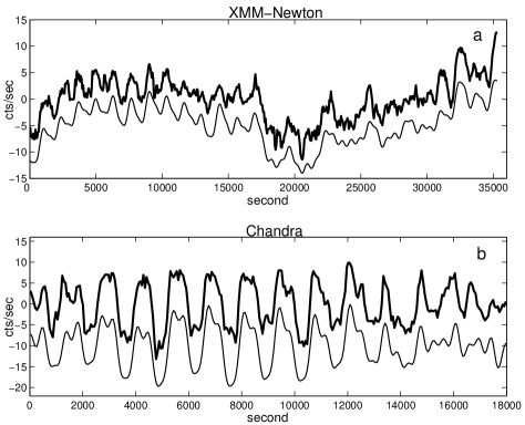
Figure 2: a) The thick curve is the X-ray light curve of V4743 Sgr obtained by binning the mean measurements of the RGS1, RGS2 and EPIC-PC detectors on board the XMM-Newton satellite into 600 equally spaced bins. The thin curve was created by Fourier series of 12 frequencies best fitted to the data by least squares. This curve is lowered by 5 units to allow comparison with the observed one. b) The thick curve is the Chandra light curve in the first 18000 s, binned into 300 bins. The thin curve shows a 6 term Fourier representation of the observed light curve (lowered by 10 units).

Table 1: List of the 12 most significant periods found in the LC of V4743 Sgr as measured by XMM-Newton, along with their respective amplitudes. The numbers in the 4th column are labels assigned to the corresponding periodicities discussed in the text. b) The same for the six most significant periodicities in the Chandra LC. The LC obtained with the XMM-Newton 12 term series and the 6 term Chandra series are shown as the thin curves in figures 2a and 2b.

Frequency	Period	Amplitude	Number
0.039412	25373	4.4757	1
0.10143	9859.2	1.3735
0.7633	1310.1	1.0578	3
0.1687	5927.6	1.0138	7
0.38063	2627.2	1.0134
0.33316	3001.6	0.95226
0.13138	7611.6	0.9179
0.72908	1371.6	0.90292	2
0.30915	3234.7	0.73275	6
0.60606	1650	0.60696
0.43798	2283.2	0.60621
1.5015	665.98	0.51516	5
Table 1.b: Chandra LETG:
0.7773	1286.5	4.7977	3
0.72108	1386.8	3.7524	2
1.4817	674.92	1.7495	5
2.2425	445.94	1.4742
0.3139	3185.7	1.4129	6
0.20202	4950.0	0.9792	7

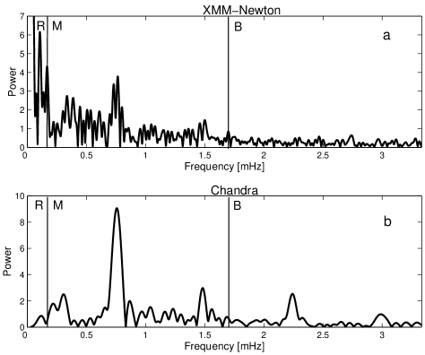
Figure 3: Upper panel: power spectrum of the XMM-Newton light curve shown in Fig. 2. Lower panel: power spectrum of the Chandra LC shown in Fig. 2. The frequency regions R, M and B are discussed in the text.

5.1 The R Spectrum

The clear difference between the two PS in the extreme red end of their frequency range reflects the obvious difference in the broad structure of the LC shown in Fig. 2. This difference is mostly due to the decline of the emission during the Chandra run, mentioned in Section 2, and the resulting detrending process that we had to apply to the Chandra LC. Due to the decline, the Chandra data do not provide us with information on the variability of the source in March 2003, on time scale longer than 6000 s, other than the decline itself.

The 36000 s long XMM-Newton observations of April, however, do show significant variability on a longer time scale. This is evident by inspection of Fig. 1 and 2, and by the high peaks in the R end of the XMM-Newton PS shown in Fig. 3. The highest peak in this band and in the entire PS is around a frequency f1=0.041 mHz. The corresponding period is P1=24300 s. Within the uncertainty in this number it is consistent with the 24380 s periodicity discovered by Wagner et al (2003) in the optical light of the nova, as mentioned in Section 2.

5.2 The M and B spectral ranges

Except for the difference in the R region, the two PS shown in Fig. 3 reveal a distinct qualitative similarity between them. The peaks in the M region are all higher than the peaks in the B band. The only two exceptions are the 3rd and the 4th harmonics of the prominent 0.75 mHz feature seen in both LC and discussed in the following section. In fact, none of the frequencies of the 20 highest peaks in the XMM-Newton PS is in the B band. In the Chandra case, among the frequencies of the 18 highest peaks, only the two harmonics of the 0.75 mHz features are in the B band and all the rest are in the M band. Using the binomial statistics formula we find that for a random uniform distribution of frequencies in our M+B band, the probability of the apparent distribution in the XMM-Newton PS is 1.8 $\times 10^{-5}$ and for the Chandra PS it is 6.5 $\times 10^{-4}$. The similarity between these two observed highly improbable frequency distributions, in the light curves obtained using entirely independent measuring devices and reduction procedures, indicates that the origin of the apparent variations in the two LC is in the source itself. Furthermore, this similarity proves that it is very likely that oscillations in X-ray flux maintained their characteristic time scale of a few thousand seconds for at least 16 days. We shall now show that precise matches of specific frequencies can also be found between the two LC, and we shall make a quantitative estimate of their statistical significance.

6 Frequency matching

6.1 Oscillation frequencies

In the M and B regions, both PS are dominated by a high feature around the frequency of 0.75 mHz. It is statistically highly significant in both PS, as evident by its large height over the noise level. Quantitatively, one can show by bootstrap analysis (Efron & Tibshirabi 1993) that in both cases, the probability for obtaining such a high peak as a result of a random process is negligibly small ($<10^{-5}$). The second harmonic of this feature around the frequency 1.5 mHz is also clearly seen in the two PS. The 3d and 4th harmonics around 2.25 and 3 mHz are also prominent in the Chandra PS, where they are also statistically significant features. The appearance and the prominence of the 0.75 mHz feature in the two PS indicate that one, or possible two cycles around this frequency probably persisted in the X-ray LC of the nova for at least 16 days, the duration of time between the Chandra and the XMM-Newton observations.

Examining only their height in the PS, all the peaks other than the 0.75 mHz and its harmonics turn out not to be statistically very significant. Each of the two observations lasted for no longer than a few to a few tens characteristic times of the apparent oscillations in the M frequency band. This is why examining the PS we cannot decisively distinguish between random noise on a time scale corresponding to this frequency band and truly periodic or quasi-periodic variability of the light source itself. However, the two X-ray observations were 16 days apart. If we find oscillations of considerable amplitude that have the same frequency in both LC, their statistical significance can be evaluated by calculating the probability of random occurrence of such coincidences.

The frequencies of peaks in the PS of a LC, especially when it is rich with many densely populated ones, may have a systematic error. In the computation of a PS of a time series, the power in each frequency measures the fitness to the data of a single harmonic oscillation with the corresponding frequency, regardless of the behavior of the LC at any other frequency. In a finite noisy time series, if the variation is also modulated by another, nearby frequency, the two frequencies may interfere. Any attempt to compare the characteristic frequencies of our 2 LC is sensitive to this possible error. In order to improve the accuracy of the frequency determination we therefore applied a least squares fitting process to the data. We used the frequency values of the highest peaks in the PS as our initial step, and by varying their values we found the set of frequencies that produces a Fourier series that fits the observed LC best in the least square sense.

Table 1 presents the 12 frequencies and periods of the highest amplitudes in a Fourier presentation of 12 or more terms that fits best the XMM-Newton light curve. It also lists the 6 frequencies of highest amplitude in the Fourier presentation of 6 or more terms of the Chandra LC. The table lists the values in a descending order of the corresponding amplitudes. The fourth column presents the labels by which we designate the periods in this paper. We note that all the 12 XMM-Newton frequencies listed in the table also coincide, as explained in detail in the next section, with frequencies that are among the 17 highest peaks in the PS of that LC. In the Chandra case, except for the B frequency of the 445 sec period, all other 5 M frequencies are among the frequencies of the highest 10 peaks in the PS of that LC.

The lower, thin curves in Fig. 2a and 2b are plots of the Fourier series of the 12 and the 6 frequencies listed in Table 1.

6.2 Coincidences

Looking for coincidences between frequencies of the XMM- Newton LC with frequencies in the Chandra LC, we must first define what we consider a coincidence. An uncertainty in the value of the frequency of an apparent oscillation in a noisy light curve is 1/T, where T is the duration of the observing run. For a LC oscillating with a given frequency, this is the half width at zero level of the peak in the PS around this frequency. We now define a frequency f(XMM) in the XMM-Newton LC as coincident with a frequency f(Chan) in the Chandra LC if the distance between the two on the frequency axis is smaller than the sum of the uncertainties in each LC divided by K, namely, if

$$|f(XMM)-f(Chan)|<{{1\over T(XMM)}+{1\over T(Chan)}\over{\rm K}}={\Delta f\over{\rm K}}$$

where T(XMM)=36000 s and T(Chan)=18000 s are the length of the corresponding LC.

Comparing numbers in the table we find that all 5 Chandra M frequencies coincide (with K=2) with 5 frequencies among the 9 XMM-Newton M frequencies. The 5 coinciding periods are labeled 2-7 in the table. Out of these 5, 4 are coincident with K=4, namely, the distance between the XMM-Newton and the corresponding Chandra frequency is smaller than 1/4th of the sum of the uncertainties in the frequency values.

6.3 Probabilities

The significance of the matches that we find between frequencies of the XMM-Newton and the Chandra LC can be evaluated by statistically testing the hypothesis that the two sets are independent of each other. Under this assumption we can calculate the probability of obtaining the number of observed matches. From a uniform distribution of numbers in the M+B band we select randomly a set of 6 numbers for Chandra and a set of 9 numbers for XMM-Newton. We then find the number of matches between these two sets, in the above mentioned sense. By repeating the sampling many thousands times, we find that the probability of obtaining 5 matches of the K=2 type, between sets of 9 and 6 frequencies in the M+B band, is $<6\times 10^{-4}$. The probability of 4 K=4 type matches is even smaller. Even if we restrict ourselves to the narrower frequency interval of just the M band alone, the probability of 5 matches is still smaller than 1.5 $\times 10^{-3}$.

We may therefore conclude, with more than 99% statistical confidence, that the two LC oscillate with the same 5 frequencies. The similarity in the frequency values, within the very small observational uncertainty limits, makes it very likely that all the 5 had stable frequencies for at least the 16 days separating the two X-ray observations.

6.4 The 0.75 mHz Feature

The 0.75 mHz dominant feature in the PS of both LC deserves a special comment. It is statistically significant in each PS alone. It indicates clearly that an X-ray source emitting a periodic or a quasi-periodic signal, contributed significantly to the emission of the source at the two observation times. In the PS of the Chandra data, this feature is unresolved and the peak in the spectrum is found at the frequency 0.755 mHz. This feature in Chandra PS is distinctly wider than other peaks, indicating that it very likely an overlap of more than a single frequency. Furthermore, our least squares fitting procedure establishes that the fit to the data with two separate frequencies, 0.728 and 0.782 mHz, is much better than with the 0.755 single frequency. The later is indeed the average of the two separated frequencies in the XMM-Newton LC. This claim is not just the trivial statement that a fit to data of a function with two free parameters is better than with one parameter only. The fit to the Chandra data with the 2 frequencies is even better than the fit with the 3 frequencies of the 3 most significant peaks in the PS of Chandra.

The f2=0.728 mHz frequency is practically the same in the XMM and the Chandra LC, although in XMM-Newton its amplitude is about 1/4th of what it was during the Chandra observations. The corresponding period is P2=1371 s. The frequencies of the second component of the 0.75 mHz feature in the two LC do not match each other as well, but they are coincident with each other by the criterion discussed in Section 6.1 with K=4 (see Table 1). The cause of the mismatch here is probably in the 18000 s modulation of the Chandra LC, imposed by the decline of the emission at the end of that run (Fig. 1d). The second frequency that we find in the 0.75 mHz feature of Chandra is close to 0.782 mHz, the frequency of the beat of a 18000 s cycle with the 0.728 frequency. As the frequency of the second component of the 0.75 mHz feature we take f3=0.763 mHz, which is the value found in the least squares fitting process, as well as in the PS of the XMM-Newton LC, where this component is well resolved. The corresponding period is P3=1310 s. Note that within a narrow margin of uncertainty in the value of the frequencies, the following relation holds:

$$f1\simeq f3-f2$$ (1)

The second harmonics of the 0.75 mHz feature is also clearly present in the PS of the two LC. In the XMM-Newton PS it is also resolved into 2 components of frequencies f4=1.459 mHz and f5=1.504 mHz. The corresponding periods are P4=685 sec and P5=665 sec. The first one satisfies the relation

$$f4\simeq 2\times f2$$ (2)

while the second one satisfies

$$f5\simeq f2+f3.$$ (3)

The 3d and 4th harmonics of the 0.75 mHz feature are also clearly present in the Chandra PS, each one as a single, unresolved peak around the mean respective frequency.

6.5 Energy dependence

As described in Section 3, from measurements by the epic-pn camera on board XMM-Newton we were able to extract 3 narrow band LC: LOW (0.2-0.4 keV), MED (0.4-0.6 keV) and HIGH ($>$0.6 ksV). These “color” LC cover only 30000 second, rather than 36000 second covered by the RGS camera. Their spectral resolution is therefore somewhat lower than that of our average LC analyzed in the previous sections. Figure 4a displays a blow-up of the PS of the average LC shown in Figure 3a, around the frequency of the 0.75 mHz feature. Figures 4b, c, and d display the same frequency interval in the power spectra of the LOW, MED and HIGH LC. The feature is resolved into 2 components in the LOW PS where the 1310 component is higher than the 1371 sec one. The feature is unresolved but appears as a single, broad peak in Figure 4c and 4d. Its profile is however clearly different in these two curves. The peak frequency in the MED PS corresponds to P=1342 sec, the peak in the HIGH PS is at the frequency corresponding to P=1367 sec. It therefore seems that there is a systematic change in the ratio of the power in the two components. At low energy the 1310 s cycle is dominating. At the mid-energy the two cycles contribute equally to the power spectrum, while at our high energy band the 1371 sec cycle takes the lead.

With the data at hand we are unable to quantify the statistical significance of this apparent trend. We do note, however, that none of the other peaks in the PS of the 3 color LC show similar variations, much less systematic ones, among the different energy bands.

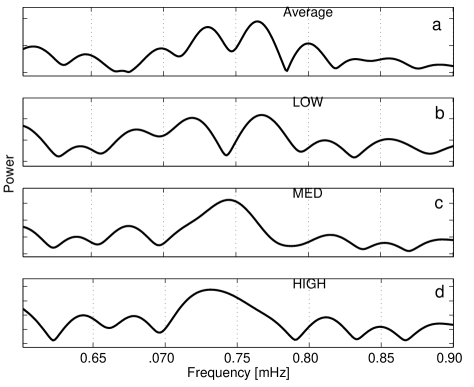
Figure 4: a) A blow-up of the frequency region around the 0.75 mHz feature in the XMM-Newtin PS shown in Figure 1a. b,c,d) The same frequency region in the PS of the LOW, MED and HIGH XMM-Newton LC.

7 Discussion

The XMM-Newton and Chandra measurements reveal that some 6 months after the outburst of nova V4743 Sgr, the supersoft X-ray flux of this object oscillated with a set of discrete frequencies. In fact, except for the decline in the emission detected in March 2003, the temporal behavior of the supersoft X-ray emission of the nova during the two observations is well interpreted as consisting entirely of oscillations in 10- 20 discrete frequencies, superimposed on some DC emission. Most of these frequencies are confined to the M frequency band. All frequencies in the B band seem to be higher harmonics of the more fundamental frequencies in the M band.

7.1 The 24000 sec cycle

The period P1=24000 s associated with the most dominant feature in the PS of the XMM-Newton LC is almost identical to the optical photometric period discovered by Wagner et al. (2003). It is tempting to identify the X-ray periodicity with the optical one but some caution is still called for since less than two complete cycles of this periodicity have been recorded in the X-ray so far. Wagner et al suggested that this is the binary period of the system. The question of the possible identification of the 24000 s with the orbital period of the nova system is of course very important. Comparison of the 2 X-ray LC indicate that if the 24000 s is indeed the binary period, then the decline observed with Chandra in March of 2003 (Ness et al. 2003, Starrfield et al. 2003) is not an eclipse related to the binary revolution. If this were true, the system would have undergone considerable geometrical changes between March 20 and April 4, which seems highly unlikely.

7.2 The two major periodicities

The P2 and P3 periodicities that constitute the 0.75 mHz feature in the PS of both LC, may be the signatures of non radial pulsations of the white dwarf of this nova system (see next section). However, their prominence in the two LC and relation (1) of Section 6.3 may indicate that their origin is different from that of the other periodicities in the LCs. We suggest that one of these two periods is the spin period of the WD. A cycle of $\simeq$1300 s is indeed a typical value of spin periods in IP systems (Hellier 2001). In Section 6.4 we showed that the ratio between the power of the P2 and P3 periodicities is energy dependent. This lends some support to the suggestion that these two frequencies originate in two different mechanisms. If one of them is a member in the family of the other major oscillations of the system, as suggested in the next section, the other is foreign to it, and the spin of the WD is a natural candidate to be its source.

If the 24000 s is the orbital period of the system, from relation (1) in Section 6.3 we see that the second period of the 0.75 mHz feature could be the orbital sideband cycle of the WD. For a prograde spin, the sidereal spin period must be the shorter of the two, namely P3=1310 s. Signals of the spin period and of its sideband have been detected in the light curves of a number of Intermediate Polar CVs (Warner 1995). An example is FO Aqr whose X-ray light curve observed with Ginga varied with two periods (Hellier 1993) . In fact even the numerical value of that WD spin period, 1254 s, and of its orbital period, 17460 s, are rather similar to our case.

Two major possibilities, well explained in Hellier (2001), may explain the orbital sideband oscillations are: a) diskless accretion by a magnetic WD, and b) reprocessing of beamed radiation from the spinning WD by an element in the binary system that is fixed in the orbital rotating frame. Even with the rich spectral information we have obtained in this observation (Ness et al. 2003), we do not find indications to discriminate between these two possibilities by analysing the spectra and variations in the depth of lines.

We shall not attempt to provide a model for the temporal characteristics of the X-ray emission of V4743 Sgr described in this work. We note, however, that on the basis of the sideband models for the f2 and f3 frequencies it is difficult to explain the presence of f5 in the PS of XMM-Newton, which satisfies relation (3) of Section 6: f5=f2+f3.

7.3 Other cyclic variations

Two other periodicities, P6 and P7 (see Table 1), persisted in the LC of the star for 16 days or more (Section 4). Taking for each the average value, weighted by the respective resolving powers, of the two measurements by Chandra and by XMM-Newton, we adopt P6=3218 sec and P7=5602 sec.

The data do not allow establishing at a statistically significant level the presence of additional periodic oscillations. It is however likely that some of the other frequencies found the two LC, e.g. the one corresponding to the 2nd highest peak in the XMM-Newton LC at P=9860 second, are also signals of periodic or quasi-periodic oscillations of the X-ray emission of the star.

Several different and simultaneous periodic or quasi periodic oscillations in the X-ray light curve have never been observed before in classical nova systems. It is tempting to suggest that at least some of the observed X-ray variability is due to white dwarf pulsations. The signature of white dwarf pulsations in the X-ray emission of classical novae has already been found for V1494 Aql (Drake et al 2003). It will be important to assess whether some of the periodicities we have detected are indeed due to nonradial pulsations of the hot WD, whose atmosphere must be extremely rich in oxygen, since the CNO cycle is on going in a thin shell underneath the atmosphere. Starrfield et al (1985) show that instabilities may occur due to ionization of carbon and oxygen and may give rise to pulsations of time scales of the order of the periodicities that we have discovered in the M band frequency range. These calculations, performed for hot stars evolving from the asymptotic giant branch to the white dwarf cooling sequence, may not be directly relevant to our case since the effective temperature of V4743 Sgr in these observations was above 500,000 K (see results obtained by Petz et al. 2005, and by Rauch & Orio 2004, Orio et al. 2005 with two different methods and models). They do point, however, toward the possibility that a similar mechanism operating on another atomic species at a higher excitation state, may produce the observed cyclic variations of our source.

Non radial pulsations of a similar time scale were also detected in the light of the hot, very evolved WD PG 1159035 and RXJ 2117.1+3412, with periods around 230-830 s (McGraw et al. 1979, Vauclair et al. 1993). WD that are nuclei of planetary nebulae have also been observed to undergo nonradial pulsations (Grauer & Bond 1984). If confirmed, nonradial pulsations of novae WD offer a new way to understand the chemical composition and temperatures of the WD and will provide new means to study the system evolution as well. X-ray observations of post- outburst novae may therefore be even more rewarding than previously thought.

8 Summary and Conclusions

Variability by up to 40% of the total X-ray flux, has been discovered in the X-ray light curve of the classical nova V4743 Sgr 6 and 6.5 months after the optical maximum. The light curve was sampled in March 2003 for 8 hours by Chandra, and 16 days later for 10 hours with XMM-Newton. It was found to vary intensely on all time scales between the duration of the observations and about 300 s. One of these variations seems to correspond to a period discovered at optical wavelengths, which was identified as the orbital period of the system.

We have found at least 5 periodicities in addition to the suspected orbital one. They appear to be the signals of oscillations with frequencies that persisted in the LC for more than 16 days. Other periodicities or quasi-periods characterize the LC as well. Some of the periods are likely to be reflections of nonradial pulsations of the atmosphere of the hot WD of the nova. Two of the periodic variations with the periods 1371 s and 1310 s are particularly intense. One of them may be the spin period of the WD of this nova system. The frequency that is the sum of these two frequencies has also been identified in the LC.

The results of our time series analysis of the XMM-Newton and Chandra observations underline the value of further, more intense time resolved photometry of this interesting nova and of classical novae in general, in the X-ray, as well as in the optical region of the spectrum.

References

- (1) Burke, B.E., et al. 1997, IEEE Trans. ED-44, 1633
- (2) Brinkman, B.C., et al. 2000, Proc. SPIE, 4012, 81
- (3) den Herder, J.W. et al. 2001, A&A, 365, L7
- (4) Drake, J.J., et al. 2003, ApJ, 584, 448
- (5) Efron, B., & Tibshirani, R.J. 1993, in An Introduction to the Bootstrap, Monographs on Statistics and Applied Probability 57, Chapman & Hall
- (6) Grauer, A.D., & Bond, H.E. 1984, ApJ, 277, 211
- (7) Haseda, K. 2002, IAU Circ. 7975
- (8) Hellier, C., 1993, MNRAS, 265, L35.
- (9) Hellier, C. 2001, ”Cataclysmic Variable Stars”, Springer-Praxis Publishing, Ch. 9.
- (10) Jansen, F., et al. 2001, A&A, 365, L1 2002, AAS 201, 40.03
- (11) Kato, T. 2002, IAU Circ. 7975
- (12) Lyke, K.E. et al 2002, Bull. AAS, Vol. 34, 1161
- (13) McGraw, J.T., Starrfield, S.G., Angel, J.R.P., & Carlton, N.P. 1979, in IAU Coll. 53, White Dwarfs and Variable Degenerate Stars, ed. H.M. Van Horn and V. Weidemann (New York: University of Rochester Press), p. 377 2000, ApJ, 545, 974
- (14) Ness, J.U., et al.. 2003, ApJ, 594, L127
- (15) Nielbock, M., & Schmidtobreick, L. 2003, A&A, 400, L5
- (16) Orio, M., Parmar, A., Greiner, J., Ögelman, H., Starrfield, S., & Trussoni, E. 2002, MNRAS, 333, L11
- (17) Orio, M., et al. 2003, IAU Circ. 8131
- (18) Orio, M., & Rauch, T. 2004 HEAD, 8, 25.26
- (19) Orio, M., Rauch, T., Tepedelenlioglu, E., & Leibowitz, E. 2005, in The Astrophysics of Cataclysmic Variables and Related Objects, J.-M. Hameury and J.-P. Lasota editors, San Francisco: Astronomical Society of the Pacific, 2005, 305
- (20) Petz, A., Hauschildt, P. H., Ness, J.-U., Starrfield, S. 2005, A&A, 431, 321
- (21) Rauch, T., Orio, M., Gonzalez-Riestra, R., & Still, M. 2005, in 14th European Workshop pn White Dwarfs, ASP Conference Series, Vol. 334, Edited by D. Koester and S. Moehler. San Francisco: Astronomical Society of the Pacific, 2005, p.423
- (22) Roberts, D.H., Lehar, J. & Drehler, J.W. 1987, AJ, 93, 968
- (23) Starrfield, S., Drake, J-J, Ness, J-U., & Orio, M. 2003, IAU Circ. 8107
- (24) Starrfield, S., Cox, A.N., Kidman, R.B., & Pesnell, W.D. 1985, ApJ, 293, L23
- (25) Strüder, L. et al. 2001, A&A, 365, L18
- (26) Turner, M.J.L. et al. 2001, A&A, 365, L27
- (27) Vauclair, G. et al. 1993, A&A, 267, L35
- (28) Warner, B., 1995, ”Cataclysmic Variable Stars”, Cambridge University Press, Ch. 7.
- (29) Wagner, R.M., et al. 2003, IAU Circ. 8176
- (30) Watson, M.G. et al. 2001, A&A 365, L36