On the migration of protogiant solid cores

Abstract

The increase of computational resources has recently allowed high resolution, three dimensional calculations of planets embedded in gaseous protoplanetary disks. They provide estimates of the planet migration timescale that can be compared to analytical predictions. While these predictions can result in extremely short migration timescales for cores of a few Earth masses, recent numerical calculations have given an unexpected outcome: the torque acting on planets with masses between $5\;M_{\oplus}$ and $20\;M_{\oplus}$ is considerably smaller than the analytic, linear estimate. These findings motivated the present work, which investigates existence and origin of this discrepancy or “offset”, as we shall call it, by means of two and three dimensional numerical calculations. We show that the offset is indeed physical and arises from the coorbital corotation torque, since (i) it scales with the disk vortensity gradient, (ii) its asymptotic value depends on the disk viscosity, (iii) it is associated to an excess of the horseshoe zone width. We show that the offset corresponds to the onset of non-linearities of the flow around the planet, which alter the streamline topology as the planet mass increases: at low mass the flow non-linearities are confined to the planet’s Bondi sphere whereas at larger mass the streamlines display a classical picture reminiscent of the restricted three body problem, with a prograde circumplanetary disk inside a “Roche lobe”. This behavior is of particular importance for the sub-critical solid cores ($M\lesssim 15\;M_{\oplus}$) in thin ($H/r\lesssim 0.06$) protoplanetary disks. Their migration could be significantly slowed down, or reversed, in disks with shallow surface density profiles.

1 Introduction

Ever since it was realized that the torque exerted by a protoplanetary disk onto an orbiting protoplanet could vary its semi-major axis on a time scale much shorter than the disk lifetime (Goldreich & Tremaine, 1979), many efforts have been made to determine the direction and rate of this semi-major axis change, referred to as planetary migration. During two decades, this problem was essentially tackled through linear analytical estimates of the disk torque onto a point-like perturber. The torque on a planet in a circular orbit can be split into two components: the differential Lindblad torque and the corotation torque. Early work on planetary migration consisted in determining the sign and value of the differential Lindblad torque in a two-dimensional disk (Ward, 1986), since this torque, in the linear regime, typically exceeds the coorbital corotation torque and therefore dictates the direction and timescale of planetary migration. This work indicated that planetary migration in most cases corresponds to an orbital decay towards the center, and that it is a fast process, thus posing a threat for the survival of protoplanets embedded in protoplanetary disks. Later efforts focused on the corotation torque (Ward, 1989) and on the disk’s vertical extent and pressure effects on the differential Lindblad torque (Artymowicz, 1993). The analytical predictions in the linear regime were checked by numerical integration of the differential equations (Korycansky & Pollack, 1993). Finally, Tanaka et al. (2002) have given an expression of the tidal torque, in the linear regime, that takes into account both the Lindblad and coorbital corotation torques, and that fully takes into account the three dimensional structure of the disk. These analytical or semi-analytical studies all consider small mass planets, for which a linear approximation of the disk response is valid. Other studies dealt with a strongly non-linear case, that of embedded giant planets (Lin & Papaloizou, 1986a, b). They showed that a giant planet tidally truncates the disk by opening a gap around its orbit, and that it is then locked in the viscous disk evolution, a process that was much later referred to as type II migration (Ward, 1997). A more recent work (Masset & Papaloizou, 2003) considers the case of sub-giant planets (planets which have a mass of the order of a Saturn mass, if the central object has a solar mass) embedded in massive disks. This work shows that the coorbital corotation torque may have a strong impact on the migration, and can lead to a runaway of the latter, either inwards or outwards. As this mechanism heavily relies upon the finite width of the horseshoe region, it also corresponds to a non-linear mechanism. The onset of non-linear effects should therefore occur below a sub-giant planet mass, but the first manifestation of these effects and their impact on planetary migration have not been investigated thus far. Korycansky & Papaloizou (1996), by writing the flow equations in dimensionless units, have shown that the flow non-linearity is controlled by a parameter ${\cal M}=q^{1/3}/h$, where $q=M_{p}/M_{*}$ is the planet mass to star mass ratio and $h=H/r$ is the disk aspect ratio. The linear limit corresponds to ${\cal M}\rightarrow 0$, while the condition ${\cal M}>1$ has been considered as a necessary condition for gap clearance, and has sometimes been referred to as the gap opening thermal criterion, although a recent work by Crida & al. (2006) has revisited the conditions for gap opening.

In the last few years, the increase of computational resources has made possible the evaluation of the disk torque exerted on an embedded planet by means of hydrodynamical calculations, both in two dimensions (Lubow et al., 1999; Nelson et al., 2000; D’Angelo et al., 2002; Masset, 2002; Nelson & Benz, 2003a, b) and three dimensions (D’Angelo et al., 2003; Bate et al., 2003), both for small mass planets and for giant planets. In particular, the case of small mass planets allows comparison with analytical linear estimates. This was done by D’Angelo et al. (2002, 2003) and Bate et al. (2003), who compared the torques they measured with the estimate by Tanaka et al. (2002). Although D’Angelo et al. (2002) and Bate et al. (2003) found results in good agreement with linear expectations, D’Angelo et al. (2003) found a significant discrepancy for planet masses in the range $5$–$20\;M_{\oplus}$. Namely, they found that migration in this planet mass range may be more than one order of magnitude slower than expected from linear estimates. In the same vein, Masset (2002) found that planetary migration for the same planet masses can be much slower, or even reversed, compared to linear estimates. Since the migration of protoplanetary cores of this mass constitutes a bottleneck for the build up of giant planets cores (as this build up is slow, while the migration of these cores is fast), it is fundamental to establish whether this effect is real and, if confirmed, to investigate the reasons of this behavior. We shall hereafter refer to this discrepancy as the offset.

We adopt for the presentation of our results a heuristic approach that consists first in presenting the set of properties that we could infer from our calculations, and then in interpreting and illustrating them through the appropriate analysis. Besides its pedagogical interest, this approach also closely follows our own approach to this problem.

In section 2.4, we describe the two independent codes that we used to check the properties of the offset, and we give the numerical setup used by each of these codes. In section 3 we list the set of properties of the offset that our numerical experiments allowed us to identify, namely:

• The offset scales with the vortensity gradient (the vortensity being defined as the vertical component of the vorticity divided by the surface density).

• The offset value varies over the horseshoe libration timescale, and tends to small values at small viscosity, whereas it remains large at high viscosity.

• The maximum relative offset occurs for a planet mass that scales as $h^{3}$.

We then interpret these properties as due to a non-linear behavior of the coorbital corotation torque that exceeds its linearly estimated value. Using the link between coorbital corotation torque and horseshoe zone drag (Ward, 1991, 1992; Masset, 2001, 2002; Masset & Papaloizou, 2003), we perform in section 4 a streamline analysis in order to check whether the coorbital corotation torque excess is associated to a horseshoe zone width excess. We find that this is indeed the case. In section 5, we relate this width excess of the horseshoe region to a transition of the flow properties in the planet vicinity, from the linear regime to the large mass case in which a circumplanetary disk surrounds the planet. We finally discuss in section 6 the importance of these properties for the migration of sub-critical solid cores. We sum up our results in section 7.

2 Hydrodynamical codes and numerical set up

We used two independent hydro-codes to perform our tidal torque estimates. One of these codes is the 3D nested grid code NIRVANA, the other one is the 2D polar code FARGO. The use of these codes was complementary: while FARGO suffers from the 2D restriction and its outcome is plagued by the use of a gravitational softening length, it enables one to perform a wide exploration of the parameter space (mainly, in our case, in term of planet mass, surface density slope, disk thickness and viscosity). The properties suggested by the FARGO runs can later be confirmed by much more CPU-demanding 3D runs with NIRVANA.

2.1 The NIRVANA code

This code is a descendant of an early version of the MHD code NIRVANA (Ziegler & Yorke, 1997), hence the name. For the current application, the magnetic terms in the MHD equations are excluded. The code features a covariant Eulerian formalism that allows to work in Cartesian, cylindrical, or spherical polar coordinates in one, two, or three dimensions. The MHD equations are solved on a staggered mesh, with a constant spacing in each coordinate direction via a directional splitting procedure, whereby the advection part and the source terms are dealt with separately. The advection of the hydrodynamic variables is performed by means of a second-order accurate scheme that uses a monotonic slope limiter (van Leer, 1977), enforcing global conservation of mass and angular momentum. Viscous forces are implemented in a covariant tensor formalism. The code allows a static mesh refinement through a hierarchical nested-grid structure (D’Angelo et al., 2002, 2003). The resolution increases by a factor $2$ in each direction from a sub-grid level to the next nested level. When employed in a 3D geometry, this technique produces an effective refinement of a factor $8$ from one grid level to the next one.

2.2 The FARGO code

The FARGO code is a staggered mesh hydro-code on a polar grid, with upwind transport and a harmonic, second order slope limiter (van Leer, 1977). It solves the Navier-Stokes and continuity equations for a Keplerian disk subject to the gravity of the central object and that of embedded protoplanets. It uses a change of rotating frame on each ring that enables one to increase significantly the time step (Masset, 2000a, b). The hydrodynamical solver of FARGO resembles the widely known one of the ZEUS code (Stone & Norman, 1992), except for the handling of momenta advection. The Coriolis force is treated so as to enforce angular momentum conservation (Kley, 1998). The mesh is centered on the primary. It is therefore non-inertial. The frame acceleration is incorporated in a so-called potential indirect term. The full viscous stress tensor in cylindrical coordinates of the Navier-Stokes equations is implemented in FARGO. A more detailed list of its properties can be found on its website.

2.3 Units

As is customary in numerical calculations of disk-planet tidal interactions, we use the planet orbital radius $a$ as the length unit, the mass of the central object $M_{*}$ as the mass unit, and $(a^{3}/GM_{*})^{1/2}$ as the time unit, where $G$ is the gravitational constant, which is $G=1$ in our unit system. Whenever we quote a planet mass in Earth masses, we assume the central object to have a solar mass. We note $M_{p}$ the planet mass and $q=M_{p}/M_{*}$ the planet to star mass ratio.

2.4 Numerical Set up

Both codes use an isothermal equation of state with a given radial temperature (or sound speed) profile. If $P$ is the (vertically integrated for FARGO) pressure and $\rho$ the (vertically integrated for FARGO) gas density, then the equation of state is $P=c_{s}^{2}\rho$. The disk vertical scale-height is $H(r)=c_{s}(r)/\Omega(r)$, where $\Omega(r)$ is the disk angular frequency at radius $r$. The disk aspect ratio, $h(r)=H(r)/r$, is taken uniform in the disks that we simulate, and it varies from $h=0.03$ to $h=0.06$ depending on the runs.

The softening length is applied to the planet potential in the following manner:

$$\Phi_{p}=-\frac{GM_{p}}{\sqrt{r_{p}^{2}+\epsilon^{2}}},$$ (1)

where $\Phi_{p}$ is the planet potential, $r_{p}$ the distance to the planet, and $\epsilon$ is the softening length.

In all the runs presented in this work, the planet is held on a fixed circular orbit. Moreover, there is no gas accretion onto the planet. This is quite different from the prescription of D’Angelo et al. (2003) and Bate et al. (2003). However, we shall see that the effect we investigate is related to the coorbital corotation torque, which itself is related to the horseshoe dynamics. In the case in which accretion is allowed, the flow topology in the planet vicinity is more complex than in a non-accreting case, with an impact on the horseshoe zone and on the coorbital corotation torque value. In order to retain only the physics relevant to the effect we are interested in, we discard gas accretion onto the planet. It should however be kept in mind that this is not realistic for planet masses $M_{p}\gtrsim 15\;M_{\oplus}$. Nonetheless, the phenomenon we describe does persist, and indeed was originally observed, when planetary cores are allowed to accrete.

In our runs the disk surface density is initially axisymmetric and has a power-law profile: $\Sigma(r)=\Sigma_{0}(r/r_{0})^{-\alpha}$, where $r_{0}=1$ is the radius at which the surface density is $\Sigma_{0}$. The kinematic viscosity has a uniform value over the disk. We have adopted a reference set up which closely resembles the one of D’Angelo et al. (2003) or Bate et al. (2003). Its characteristics are listed in Table 1. Whenever we vary one disk parameter (e.g. aspect ratio or viscosity), we adopt for the other parameters the reference values. For a given set of disk parameters, we perform several calculations with different planet masses.

Table 1: Disk parameters for the reference calculations. There is no accretion onto the planets.

Parameter	Notation	Reference value
Aspect ratio	$h$	$0.05$
Surface density slope	$\alpha$	$1/2$
Viscosity	$\nu$	$10^{-5}$

We list below the details specific to each code:

• In the 3D-NIRVANA runs, the computational domain is a spherical sector $[R_{\mathrm{min}},R_{\mathrm{max}}]\times[\theta_{\mathrm{min}},\theta_{\mathrm{max}}]\times 2\pi$, whose radial boundaries are $R_{\mathrm{min}}=0.4$, $R_{\mathrm{max}}=2.5$. Symmetry is assumed relative to the disk mid-plane and only the upper half of the disk is simulated, hence $\theta_{\mathrm{max}}=90^{\circ}$. The minimum co-latitude, $\theta_{\mathrm{min}}$, varies from $80^{\circ}$ to $82.5^{\circ}$, according to the value of the aspect ratio $h$. The vertical extent of the disk comprises at least $3$ pressure scale-heights. Outgoing-wave (or non-reflecting) boundary conditions are used at the inner radial border (Godon, 1996). In order to exploit the mirror symmetry of the problem with respect to the disk equatorial plane (the disk and the planet orbit are coplanar), a symmetry boundary condition was used at the disk mid-plane, which enables us to simulate only the upper half of the disk. Finally, reflecting boundary conditions were used at the outer radial border, which is located sufficiently far from the orbit so that the wake reflection will not alter our torque evaluation, and at $\theta=\theta_{\mathrm{min}}$, were the matter is so rarefied that the choice of the boundary condition has virtually no impact on the flow properties on the bulk of the disk. The reference frame has its origin on the center of mass of the star-planet system and corotates with the planet. The grid hierarchy consists of a basic mesh with $(N_{R},N_{\theta},N_{\phi})=(143,13,423)$ grid zones and $4$ additional sub-grid levels centered at the planet’s position, each with $(64,12,64)$ grid zones. The initial vertical density distribution is that of an unperturbed disk in hydrostatic equilibrium, which in spherical coordinates reads $\rho(t=0)=\rho_{0}(R)\,\exp{[(\sin{\theta}-1)/h^{2}]}/(\sin{\theta})^{(\alpha+1)}$, where $\rho_{0}\propto 1/R^{(\alpha+1)}$ and the sound speed is assumed to scale as $c_{s}\propto h/\sqrt{R\sin{\theta}}$. Such density profile is stationary in the limit $M_{p}\rightarrow 0$. The initial surface density, obtained by integrating the mass density in $\theta$, is $\Sigma=\Sigma_{0}(a/R)^{\alpha}$, where $\Sigma_{0}=2.9\times 10^{-4}$. Calculations were performed for many values of the planet to star mass ratio, from $q=10^{-6}$ to $q=2\times 10^{-4}$, in disks with various values of the initial density slope $\alpha$, aspect ratio $h$, and kinematic viscosity $\nu$. Simulations were run for up to $140$ orbital periods to measure (partially) saturated coorbital corotation torques. Shorter runs ($10$ orbits) were used to monitor (partially) unsaturated corotation torques. In 3D calculations, torques arising from the Roche lobe are not very sensitive to the choice of the softening parameter, $\epsilon$, in the planet gravitational potential, as long as it is a small fraction of the Hill radius $R_{H}=a(q/3)^{1/3}$. We used $\epsilon=0.1R_{H}$. However, some models were also run with a smaller softening length and produced no significant differences.

• In the 2D-FARGO runs, the mesh inner boundary is at $R_{\rm min}=0.5$ and the mesh outer boundary is at $R_{\rm max}=2.1$. A non-reflecting boundary condition was used at each boundary. The resolution is of $N_{\rm rad}=153$ zones in radius and $N_{\phi}=600$ zones in azimuth. The mesh spacing is uniform both in radius and in azimuth. The frame corotates with the planet. The value of $\Sigma_{0}$ is $6\cdot 10^{-4}$. The potential softening length is $\epsilon=0.3H$. This value is quite low. Preliminary calculations have shown that the offset is much larger at small potential softening length value, which is why we adopted this value. For a given set of disk parameters, we performed 35 calculations with 35 different planet masses, in geometric sequence and ranging from $q=10^{-6}$ to $q=10^{-3.5}$: $q_{i}=10^{-6+2.5i/34}$, $0\leq i\leq 34$. Most of the calculations are run for 100 orbits, in order for the coorbital corotation torque to saturate if the disk parameters imply its saturation. We have also performed series of short runs for 10 orbits, in order to have an unsaturated corotation torque.

2.5 Torque evaluation

• In the 3D runs, the gravitational torques acting on the planet are evaluated either every $5$ orbits (long-run simulations) or every orbit (short-run simulations). In the first case, the total torque is averaged over the last $30$ orbital periods of the calculation whereas, in the second case, it is averaged from $t=7$ and $t=10$ orbits. As mentioned in section 2.4, accretion onto the planetary core is not allowed. In the low mass limit, this leads to the formation of a gas envelope around the planet. The size of the envelope depends on the core mass and is a fraction of $R_{H}$. To avoid the envelope region, torque contributions from within the Hill sphere were discarded. This choice may occasionally result in some corotation torques being unaccounted for. When this happens, the departure from the linear regime may be underestimated. However, tests performed by excluding torques from a region of radius $0.5R_{H}$ indicate that the effects would not significantly change the results of this study. Therefore, this choice is conservative since it may occasionally underestimate the excess of coorbital corotation torques but assures that our analysis is not affected by spurious torques from material possibly bound to the core.

• In FARGO, the torque exerted by the disk onto the planet is evaluated every $1/20^{th}$ of orbit. In the long runs case ($100$ orbits), the torque value is averaged from $t=40$ to $t=100$ orbits, in order to discard any transient behavior at the beginning of the calculation, due to corotation torque (possibly partial) saturation on the libration timescale. In the short runs case, we generally take (unless otherwise stated) the torque average between $t=6$ and $t=7$ orbits. We also entertained the issue whether the Roche lobe material must be taken into account. The FARGO code, in its standard version, outputs both the torque exerted by the totality of the disk onto the planet, without a special treatment of the Roche lobe material, and the torque obtained by tapering the torque arising from the Roche lobe and its surroundings by $1-\exp[-(r_{p}/R_{H})^{2}]$, where $r_{p}$ is the zone center distance to the planet. We show in section 3 that taking or not the Roche lobe content into account does make a difference, but that qualitatively one obtains the offset properties in both cases. We have chosen to include the Roche lobe content in the torque evaluation for the FARGO calculations presented in this work. There is another reason for this choice, namely that the material that should be discarded in the torque calculation should be the one pertaining to the circumplanetary disk: one would define the system of interest as {the planet + the circumplanetary disk}. If the circumplanetary disk has a radius that scales with $R_{H}$ and that amounts to several $0.1R_{H}$ for large planet masses, this is not true for the small planet masses that represent most of the mass interval over which we perform the calculations. For these small masses, the circumplanetary disk has a radius much smaller than a few $0.1R_{H}$, or may not even exist, as we shall see in section 5.

3 Offset properties

3.1 Reference run

3.1.1 2D results

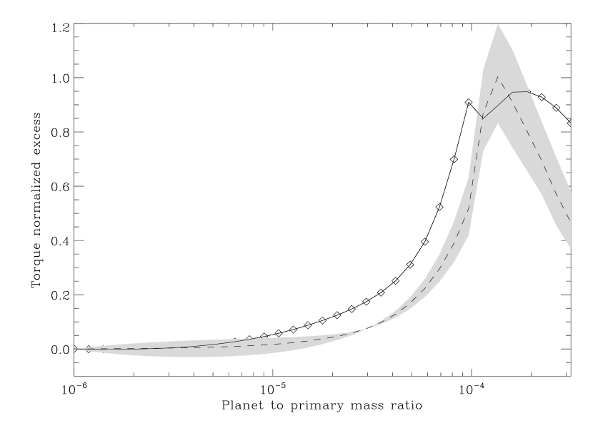
Fig. 1 shows the results of the reference run, corresponding to the parameters of Table 1, both with and without Roche lobe tapering. Both curves show the offset near $q=10^{-4}$. However the curves do not coincide, and the offsets have slightly different shapes, which indicates that it is due to material located inside of the Hill sphere or in its immediate vicinity.

As mentioned in the Introduction, previous two-dimensional simulations by D’Angelo et al. (2002) have apparently missed the offset feature shown in Figure 1. The most likely reason why this happened is the use of an extremely small softening parameters (on the order of $0.02R_{H}$), associated with the action of torques deep inside the planet’s Hill sphere (at distances from the planet $r_{p}\lesssim 0.2R_{H}$). We shall see in section 5 that for such a small softening length we should expect the offset feature to peak at $q<10^{-6}$, which is not in the mass range covered by D’Angelo et al. (2002). Furthermore, their analysis is complicated by the inclusion of accretion and the presence of a gap or dip in the initial surface density profile. We also performed a set of calculations with NIRVANA in 2D mode, using the reference parameters and adopting a setup similar to that of FARGO. The resulting specific torque versus the planetary mass is consistent with the solid line with diamonds in Figure 1.

Figure 1: Negative specific torque acting on the planet, as a function of its mass, in the reference disk for the 2D case. The solid line with diamonds shows the torque computed with Roche lobe tapering, while the dashed line shows the torque computed without special treatment of the Roche lobe zones. The solid line with stars shows the results of the three dimensional calculations, scaled by $\Sigma_{0}^{2D}/\Sigma_{0}^{3D}=60/29$. We note that the offset depth is larger in the 3D case.

3.1.2 3D results

The behavior of the total specific torque exerted by the planet on a three-dimensional disk, for the parameters given in Table 1, is illustrated in Figure 1. The departure from the total torque predicted by the linear theory is largest at $q=5\times 10^{-5}$. A comparison between Figure 1 and Figure 6 in D’Angelo et al. (2003) allows to evaluate the impact of core accretion on the excess of corotation torques. This represents an important issue since around $10\;M_{\oplus}$ the runaway gas accretion phase is most likely to occur (e.g., Wuchterl, 1993; Pollack et al., 1996; Hubickyj, Bodenheimer, & Lissauer, 2005). Accretion on the planet seems to enhance the excess of coorbital corotation torques, over the predictions based on the linear regime, since it affects the width of the horseshoe region. The location where the offset is maximal recedes from $q=5\times 10^{-5}$, when cores are non-accreting, to $q=3\times 10^{-5}$, when cores accrete at maximum rate.

3.2 Dependence on the vortensity gradient

3.2.1 2D results

Fig. 2a shows the results of a set of calculations with four different disks, having different surface density slopes. The set that exhibits the smallest departure to a linear trend (straight line) corresponds to $\alpha=3/2$, i.e. to a flat vortensity profile, since $d\log(\Sigma/B)/dr=3/2-\alpha$.

Fig. 2b shows the quantity

$$E_{\alpha}(q)=1-\frac{T_{\alpha}(q)}{q^{2}}\frac{q_{\rm min}^{2}}{T_{\alpha}(q_{\rm min})},$$ (2)

where $T_{\alpha}(q)$ is the disk torque on the planet with planet to star mass ratio $q$ when the disk surface density slope is $\alpha$, and $q_{\rm min}$ is the minimal mass ratio in our sample (here $q_{\rm min}=10^{-6}$). Whenever the disk response is linear, the torque scales with $q^{2}$ and $E_{\alpha}$ vanishes. The quantity $E_{\alpha}(q)$ is therefore a measure of the departure from linearity of the torque. It reaches unity when the total torque cancels out, and exceeds one when migration is reversed. From Fig. 2b we can see that for $q>10^{-4}$, the torque value differs from its linearly extrapolated value, regardless of the vortensity slope. For smaller masses, the departure from the linearly predicted value is larger for larger vortensity slopes. Although the flat surface vortensity profile ($\alpha=3/2$) does not have a vanishing $E_{\alpha}$, it is nevertheless the profile that exhibits the smallest departure to linear prediction (by at most 10 % up to $q\sim 1.5\cdot 10^{-4}$). The dashed and dotted line show the curve of $E_{0}$ for the flat surface density profile (maximal vortensity slope) respectively scaled by $2/3$ and $1/3$. These curves show that the departure to linearity approximately scales with the vortensity slope.

Figure 2: 2D results. Left: Negative of specific torque acting on the planet, as a function of its mass, for four values of the surface density slope: $\alpha=0$ (diamonds), $\alpha=1/2$ (reference calculation, triangles), $\alpha=1$ (squares) and $\alpha=3/2$ (crosses). The hole in the data for the flat surface density profile corresponds to a torque reversal. Right: departure from linearity for the same surface density slopes (same symbols). The meaning of the additional lines is explained in the text.

3.2.2 3D results

Figure 3: 3D results. Left. Negative of the specific torque exerted on the planet, as a function of its mass, for different values of the surface density slope: $\alpha=0$ (asterisks), $\alpha=1/2$ (diamonds), $\alpha=3/4$ (triangles), and $\alpha=3/2$ (pentagons). The gap in the data for the $\alpha=0$ case corresponds to situations where the total torque is positive. Right. Departure from linearity (Eq. 2) for the same values of $\alpha$ (same symbols identify same models).

The left panel of Figure 3 shows the specific torque exerted by the disk on the planet, obtained from 3D calculations with different surface density slopes, $\alpha$. Torques are (partially) saturated, which means that they have reached their steady state value, which is a fraction of their initial (unsaturated) value. The behavior of the quantity $E_{\alpha}$ is illustrated in right panel for the same models. As observed in the 2D results, the departure from the linear (type I) regime, increases with increasing vortensity gradient.

3.3 Dependence on the viscosity

The previous section suggests that the offset is linked to the coorbital corotation torque, since it scales with the vortensity gradient across the orbit. For the vortensity slopes considered, the coorbital corotation torque acting on the planet is positive. Note that as the offset corresponds to a positive value added to the linearly expected torque value, this would suggest that the offset corresponds to a corotation torque larger than predicted by the linear analysis. If the offset is indeed due to the corotation torque, then it should depend on the disk viscosity, since the corotation torque depends on it (Ward, 1992; Masset, 2001, 2002; Balmforth & Korycansky, 2001; Ogilvie & Lubow, 2003). We have undertaken additional sets of calculations, in which we take the reference values of Table 1, except that we vary the disk viscosity $\nu$.

3.3.1 2D results

We have taken twice the viscosity reference value ($\nu=2\cdot 10^{-5}$), and half the reference value ($\nu=5\cdot 10^{-6}$). The results are presented in Fig. 4.

Figure 4: Left: Specific torque acting on the planet as a function of the planet mass for different disk viscosities: $\nu=5\cdot 10^{-6}$ (triangles), $\nu=10^{-5}$ (reference calculations, diamonds), $\nu=2\cdot 10^{-5}$ (squares). The curve with crosses shows the torque of the reference calculations averaged between $t=6$ and $t=7$ orbits, i.e. the early value of the torque, before it possibly saturates. Right: The value of $E_{\alpha}$ (given by Eq. 2) for these calculations (same symbols).

The trend observed on this figure is compatible with the saturation properties of the corotation torque. The largest offset is observed for the early torque value, i.e. the unsaturated one, while as the viscosity decreases the departure from linearity decreases as well. Quantitatively, the behavior observed is also in agreement with a corotation torque saturation. The latter depends on the ratio of the libration timescale in the horseshoe region and the viscous timescale across it (Ward, 1992; Masset, 2001, 2002). We can for instance evaluate how saturated the corotation torque should be for $q=10^{-4}$. The horseshoe zone half width $x_{s}$ for such planet mass in a disk with $h=H/r=0.05$ can be estimated by equating the linear estimate of the coorbital corotation torque (Tanaka et al., 2002) and the horseshoe drag (Ward, 1991, 1992; Masset, 2001). One is led, in a two-dimensional disk, to:

$$x_{s}=1.16a\sqrt{\frac{q}{h}}.$$ (3)

This yields here $x_{s}=0.052$. The ratio ${\cal R}$ defined by Masset (2001) is therefore ${\cal R}=0.07$ for the reference run, ${\cal R}=0.14$ for the larger viscosity run, and ${\cal R}=0.035$ for the lower viscosity run. To within a numerical factor, ${\cal R}$ represents the ratio of the libration timescale to the viscous timescale across the horseshoe region, and therefore indicates whether the corotation torque should saturate (at low ${\cal R}$) or remain unsaturated (at higher ${\cal R}$). From Fig. 2 of Masset (2002), one can infer that the coorbital corotation torque should be about $40$ % of its unsaturated value for the smaller viscosity calculation, $60$ % for the reference calculation, and $80$ % for the larger viscosity calculation. The scatter of the curves of Fig. 4b is roughly compatible with these expectations. We note in passing that (i) this estimate is only an order of magnitude estimate, since we inferred the value of $x_{s}$ from linear calculations, whereas we suspect the offset to be due to a corotation torque value that differs from the linear estimate and (ii) it is by chance that the reference calculation, which takes the parameters of D’Angelo et al. (2003) and Bate et al. (2003), corresponds precisely to a corotation torque that is half saturated, so that varying slightly the viscosity with respect to the reference one yields a strong variation of the offset amplitude. We finally note that the saturation of the corotation torque depends on the planet mass, for a fixed viscosity. The smaller the planet mass, the less saturated is the corotation torque. We observe this behavior in Fig. 4b. Quite surprisingly however, the torque is found to depend (weakly) on the viscosity at very small $q$, whereas one would expect the corotation torque to be unsaturated. The evolution of the surface density profile is too weak to account for this observation. We have not investigated further this behavior, which we believe to be of minor importance for the work presented here. Nevertheless, we suggest that it is linked to a drop of the coorbital corotation observed by Masset (2002), when the viscosity is larger than the so-called cut-off viscosity, which corresponds to the viscosity for which the time needed by a fluid element to drift from the separatrix to the corotation is also half the libration time of this fluid element. This limit viscosity $\nu_{l}$ is given by $\nu_{l}\sim x_{s}^{2}\Omega_{p}/4\pi$ (Masset, 2001, 2002). Using Eq. (3), this translates into $\nu_{l}\sim 0.1a^{2}\Omega_{p}q/h$. We should observe a drop of the corotation torque (and therefore a dependence of the torque on the viscosity) for $\nu\gtrsim\nu_{l}$, i.e. for $q\lesssim q_{l}\sim 10h\nu/(a^{2}\Omega_{p})$. For the reference calculation, we have $q_{l}\sim 5\cdot 10^{-6}$, while we get twice and half this value for the higher and lower viscosity runs, respectively. The curves of Fig. 4a are roughly compatible with these expectations, although around $q\sim 10^{-5}$ it is difficult to disentangle this effect from the onset of the departure from linearity of the torque.

3.3.2 3D results

Figure 5: Negative of the specific torque acting on the planet, as a function of its mass, for models with $\alpha=0$. Asterisks indicate torques, from long-run simulations, for which corotation torques are saturated. Diamonds represent torques at early times (between $7$ and $10$ orbits), hence corotation torques are unsaturated.

As explained above, torques evaluated at early times contain coorbital corotation torques that are unsaturated and thus their effect is the strongest. At later evolutionary times, the effects of corotation torques may tend to weaken. Figure 5 illustrates the behavior of saturation on the total specific torque, as a function of the planet mass, obtained from calculations with a flat initial surface density ($\alpha=0$). The asterisks represent torques measured around $100$ orbits, when corotation torques are partially saturated whereas diamonds refer to torques measured between $7$ and $10$ orbits, before saturation occurs. The offset reduces as corotation torques saturate. The planet mass for which the offset is maximum shifts towards larger values and the range of masses in which the total torque is positive shrinks (see Fig. 5). However, a finite mass interval persists in which the departure from the linear regime can still be very large.

3.4 Dependence on the disk thickness

The two previous sections strongly suggest that the offset is indeed a physical effect, independent on the code used, and that it is linked to an excess of the coorbital corotation torque with respect to its linearly estimated value. This therefore implies that the offset corresponds to the onset of non-linear effects in the flow. The flow non-linearity depends on the parameter ${\cal M}=q^{1/3}/h$ (Korycansky & Papaloizou, 1996). The onset of this behavior should therefore be observed for a planet to primary mass ratio $q\propto h^{3}$. We have undertaken additional series of calculations in which we take the reference parameters of Table 1, except that we vary the disk aspect ratio.

3.4.1 2D results

We ran series of calculations with $h=0.035$, $h=0.04$, $h=0.045$, $h=0.055$ and $h=0.06$, in addition to the reference calculation with $h=0.05$. For each series, we estimate the mass for which the departure to linearity given by Eq. 2 is maximal. We refer to this mass as the critical mass, and we denote $q_{c}$ its ratio to the primary mass. This mass is determined from a parabolic interpolation of the data point which has the largest departure and its two neighbors. Since the disk viscosity is kept constant and equal to its reference value in all these calculations, and since the critical mass varies between two sets of calculations, we expect different saturation levels of the coorbital corotation torque at the critical mass, on the long term. This could mangle our analysis, and it is therefore important to take the unsaturated torque value. This is why the $E_{\alpha}(q)$ values in the analysis of this section are evaluated using the torque value averaged between $t=3$ and $t=5$ orbits. The results are presented in Fig. 6.

Figure 6: Critical mass $q_{c}$ for maximal offset as a function of the disk thickness, for the 2D runs. The dotted, dashed and dot-dashed lines show respectively the relationships $q_{c}\propto h^{2}$, $q_{c}\propto h^{4}$ and $q_{c}\propto h^{3}$ that pass through the leftmost data point. The error bars indicate the sampling of data points around the critical mass.

We see on this figure that there is an excellent agreement between the results of the calculations and the expectation $q_{c}\propto h^{3}$. This is a strong point in favor of our hypothesis that this behavior is due to the onset of non-linear effects.

3.4.2 3D results

Figure 7: Negative of the specific torque acting on the planet as a function of the planet to primary mass ratio, for different values of $h$: $0.06$ (asterisks), $0.05$ (triangles), $0.04$ (diamonds), and $0.03$ (circles). Torques are measured at early times (between $7$ and $10$ orbits) so that corotation torques are unsaturated. Gaps in the curves identify the ranges of planetary masses for which the total torque is positive.

In order to examine the dependence of the offset on the disk aspect ratio, we set up 3D models with an initial surface density slope equal to $\alpha=0$ and a relative disk thickness $h$ ranging from $0.03$ to $0.06$. For each value of $h$, a series was built by varying the planet to star mass ratio, $q$, from $10^{-6}$ to $2\times 10^{-4}$. The specific torque as a function of the planet mass, for selected disk aspect ratios, is shown in Figure 7. In thinner (i.e., colder) disks, the offset of corotation torques moves towards smaller planetary cores. When $h=0.03$, the effects of the offset are dominant between $q\approx 10^{-5}$ (or about $3\;M_{\oplus}$) and $q\approx 2\times 10^{-5}$ (or about $6\;M_{\oplus}$), regardless of the saturation level of corotation torques.

Figure 8: Critical mass versus the relative disk thickness obtained from 3D calculations. At $q=q_{c}$, the offset is the largest. The error bars indicate the sampling of the data points around the critical mass. The dashed line identifies the relationship $q_{c}\propto h^{3}$ passing through the data point with minimum $h$.

From each series, the critical mass ratio $q_{c}$ was estimated by means of a parabolic interpolation, as done for the 2D calculations. For this analysis we used total torques averaged between $t=7$ and $t=10$ orbits, i.e. before the corotation torque possibly saturate, for the reasons clarified in the previous section. The dependence of the critical mass ratio on the disk thickness is illustrated in Figure 8, along with the curve $q_{c}/q_{c}(h=0.03)=(h/0.03)^{3}$ (dashed line). The error bars indicate the sampling of the data points around the critical mass and thus represent the largest possible error on the estimates of $q_{c}$. It is evident that 3D numerical results accurately reproduce the $h^{3}$-scaling expected to arise from non-linear effects in the corotation region.

4 Streamline analysis

The calculations shown at the previous section strongly suggest that the offset is a physical effect, and that non-linear effects boost the corotation torque value with respect to its linearly estimated value. There is a link between the coorbital corotation torque and the so-called horseshoe drag (Ward, 1991, 1992; Masset, 2001, 2002), which is the torque arising from all the fluid elements of the horseshoe region. Although the corotation torque and the horseshoe drag have same dependency on the disk and planet parameters, and although the horseshoe drag may result in a very effective concept for some aspects of planetary migration related to coorbital material (Masset & Papaloizou, 2003), there is no reason why these two quantities should be exactly the same. In particular, in the low mass regime, the horseshoe region can be arbitrarily radially narrow, while the corotation torque always arises, in the linear limit, from a region of width $\sim H$, which corresponds to the length-scale over which the disturbances in the corotation vicinity are damped. Nevertheless, it is instructive to investigate whether the behavior found is linked to a boost of the horseshoe region width w.r.t. its linearly estimated width. We recall the horseshoe drag expression (Ward, 1991, 1992; Masset, 2001):

$$\Gamma_{HS}=\frac{3}{4}x_{s}^{4}\Omega_{p}^{2}\Sigma\cdot\frac{d\log(\Sigma/B)}{d\log r},$$ (4)

where $x_{s}$ is the half width of the horseshoe region, $\Omega_{p}$ is the planet orbital frequency and $\Sigma$ is the disk surface density at the orbit. Since, in the linear limit, the torque scales with the square of the planet mass, we expect the dependency $x_{s}\propto q^{1/2}$ (see also Ward (1992)). On the large mass side we may expect, that the horseshoe region has a behavior similar to the one of the restricted three body problem (RTBP) and that we have the scaling $x_{s}\propto q^{1/3}$. We performed an automatic streamline analysis on the flow of the 2D reference runs, in the frame corotating with the planet, after $t=10$ orbits (an early stage in order to avoid, on the large mass side, a radial redistribution of the disk material that alters the streamlines and hence the horseshoe zone width, but still sufficiently evolved so that the flow can be considered steady with a good approximation in the corotating frame), in order to find the separatrices of the horseshoe region by a bisection method. We show in Fig. 9 the half width of the horseshoe region as a function of the planet mass. We see on this figure that:

• the horseshoe zone width indeed scales as $q^{1/2}$ as long as the planet mass remains sufficiently small, since the data points and the dashed line have same slope for $q<3\cdot 10^{-5}$;

• there is a correct agreement between the coorbital corotation torque and the horseshoe drag, since the data points and the dashed curve, obtained from Eq. (3) by assuming a strict equality between horseshoe drag and linearly estimated coorbital corotation torque, nearly coincide on this mass range.

• We also see how the horseshoe zone width scales with $q^{1/3}$ on the large mass side, as expected. The width displayed on the dotted line however differs from the horseshoe width of the RTBP. The latter is $x_{s}=\sqrt{12}a(q/3)^{1/3}$, while we find that the data points are correctly fitted by $x_{s}\simeq 2.45a(q/3)^{1/3}$, i.e. the horseshoe width is $\sim 1.4$ times narrower than in the RTBP.

• In between the linear range and the $q^{1/3}$ scaling range, that is for $3\cdot 10^{-5}<q<1.5\cdot 10^{-4}$, the horseshoe zone width falls between the two regimes, which makes it larger than its linearly estimated value for any $q>3\cdot 10^{-5}$. This corresponds precisely to the mass for which migration becomes slower than linearly estimated.

Figure 9: Horseshoe zone half width as a function of the planet mass for the $35$ planets of the reference calculations. The dashed line represents the horseshoe zone half width expected from Eq. (3). It scales with $q^{1/2}$. The dotted line shows the relationship $x_{s}\propto q^{1/3}$ that passes through the large mass data points.

In order to finally assess whether the torque offset can indeed be due to the excess of the horseshoe zone width, we can directly estimate the excess of horseshoe drag (w.r.t. the linearly extrapolated value):

$$\Delta\Gamma_{HS}(q)=\Gamma_{HS}(q)-\Gamma_{HS}(q_{min})\left(\frac{q}{q_{min}}\right)^{2},$$ (5)

and compare it to the total torque excess:

$$\Delta T(q)=T(q)-T(q_{min})\left(\frac{q}{q_{min}}\right)^{2}=\frac{|T(q_{min})|}{q_{min}^{2}}E_{\alpha}(q).$$ (6)

Figure 10: Horseshoe drag (dashed line) and total torque (solid line) normalized excesses as a function of planet mass. The shaded area shows the uncertainty on the horseshoe drag, arising from the uncertainty on the horseshoe zone width. If one calls $x_{s}^{-}$ (resp. $x_{s}^{+}$) the distance of the inner (resp. outer) separatrix to the corotation, then the upper (resp. lower) limit of the shaded zone is given by using $\max(x_{s}^{-},x_{s}^{+})$ (resp. $\min(x_{s}^{-},x_{s}^{+})$) in Eq. (4), while the dashed line uses $(1/2)(x_{s}^{-}+x_{s}^{+})$.

The results are displayed in Fig. 10, in which we divide the torque values by $q^{2}$. We see that the horseshoe drag excess and the total torque excess exhibit the same behavior and have a very similar value in the mass range $10^{-4}<q<2\cdot 10^{-4}$, which is a quantitative confirmation that the torque excess of the offset maximum is attributable to the horseshoe zone width excess. We note that although the two curves display a similar behavior for $q<10^{-4}$, they do not coincide on this mass range, and that the total torque excess is systematically larger than the horseshoe drag excess. It is precisely for this mass range ($q<10^{-4}\sim h^{3}/1.16^{2}$, see Eq. 3) that the horseshoe zone width is narrower than the disk thickness, so that not all the coorbital corotation torque arises from the horseshoe region.

5 Flow transition

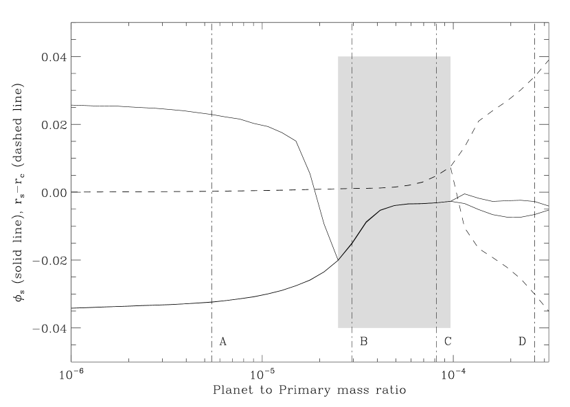
The previous section shows that the torque offset is due to a transition of the corotational flow, which has a horseshoe zone width $\propto q^{1/2}$ in the linear regime whereas it scales as $q^{1/3}$ in the large mass regime. Fig. 11 shows the streamline topology for different masses (A: $q=5.44\cdot 10^{-6}$; B: $q=2.96\cdot 10^{-5}$; C: $q=8.16\cdot 10^{-5}$; D: $q=2.67\cdot 10^{-4}$). The linear case (A) shows two stagnation points located almost at corotation, and offset in azimuth from the planet. These two stagnation points are not symmetric w.r.t. the planet, and are not located on the same streamline. As long as we are in the linear regime, they remain essentially at the same location. Then, as the planet mass increases, both stagnation points move towards the planet. The central libration region defined by the separatrix of the right stagnation point shrinks until it disappears, in which case we only have one stagnation point (case B). As the planet mass still increases, this unique stagnation point moves towards smaller azimuth while it recedes radially from the orbit (case C), then for larger masses one gets two stagnation points practically on the star-planet axis, which yields a picture very similar to the RTBP, where the stagnation points are reminiscent of the Lagrange points L₁ and L₂, and a prograde circumplanetary disk appears within the “Roche lobe” (case D). This corresponds to the regime in which the horseshoe zone width scales with $q^{1/3}$.

One could argue that despite the larger resolution adopted for the streamline analysis, the radial resolution $\delta r=(R_{\rm max}-R_{\rm min})/N_{\rm rad}=3.63\cdot 10^{-3}$ is still too coarse to properly describe the corotational flow of the small mass planets, as it amounts to a significant fraction of the horseshoe zone width. Fig. 12 shows the flow for $q=5.44\cdot 10^{-6}$ (case A) run with ten times higher a radial resolution ($N_{\rm rad}=3860$, hence $\delta r=3.63\cdot 10^{-4}$). The excellent agreement between the streamlines obtained with the two different radial resolutions confirms a fact already noted by Masset (2002), that even a low or mild radial resolution associated with a bilinear interpolation of the velocity fields allows to capture correctly the features of the corotation region.

These flow properties are illustrated in Fig. 13, which shows both the azimuth and the distance to corotation of the stagnation point(s). We see that for $q<2\cdot 10^{-5}$ we have two stagnation points located at corotation and on each side of the planet (i.e. one at negative azimuth, and one at positive azimuth). Around $q\sim 2\cdot 10^{-5}$, the stagnation points coalesce on a narrow mass interval. Up to $q\sim 10^{-4}$, there is a unique stagnation point located slightly beyond corotation and at a small, negative azimuth. Finally, at $q\approx 10^{-4}$, another bifurcation occurs, and one recovers two stagnation points on either side of corotation, and almost aligned with the star ($|\phi_{s}|\ll|r_{s}-r_{c}|/a$).

Figure 11: Streamline appearance for the four planet masses quoted in text, at $t=10$ orbits. The radial range is the same for cases A and B, and for cases C and D. It is ten times larger for the latter than from the former. The aspect ratio is $1:1$ for the cases C and D.

Figure 12: Streamline appearance for the planet mass A quoted in text, at $t=10$ orbit, with a radial resolution ten times higher than in Fig. 11. The streamlines appearance and the position of the stagnation points is almost indistinguishable from the lower resolution case. The square shows a zone from the high resolution mesh.

Figure 13: Azimuth $\phi_{s}$ of the stagnation point(s) (solid line) and radial distance to corotation ($r_{s}-r_{c}$) of the fixed point(s) (dashed line) as a function of the planet mass. The gray shaded zone shows the mass interval over which there is a unique stagnation point. The four vertical dot-dashed lines show the masses for which the flow topology is sketched in Fig. 11.

For a given finite potential softening length, there is a mass limit under which a 2D flow is linear everywhere, even at the planet location. A simple estimate of this mass limit can be found as follows. The effective potential that dictates the motion of fluid elements is $\tilde{\Phi}=\Phi+\eta$, where $\Phi$ is the gravitational potential and $\eta$ is the gas specific enthalpy. The latter reads $\eta=\eta_{0}+\eta^{\prime}$, where $\eta_{0}$ is the fluid specific enthalpy of the unperturbed flow, which is a uniform quantity as the disk has initially a uniform sound speed and a uniform surface density, and where $\eta^{\prime}=c_{s}^{2}\log(\Sigma/\Sigma_{0})$ is the perturbation of the specific enthalpy introduced by the planet. Similarly, the gravitational potential can be written as $\Phi=\Phi_{*}+\Phi_{p}$, where $\Phi_{*}$, the gravitational potential of the central star, corresponds to the unperturbed flow and where $\Phi_{p}$, the gravitational potential of the planet, corresponds to the perturbation. Hence the effective potential can be decomposed as $\tilde{\Phi}=\tilde{\Phi}_{0}+\tilde{\Phi}^{\prime}$, where $\tilde{\Phi}_{0}=\Phi_{*}+\eta_{0}$ is its value in the unperturbed flow while $\tilde{\Phi}^{\prime}=\Phi_{p}+\eta^{\prime}$ is its perturbed value.

Figure 14 shows that the two quantities $\Phi_{p}$ and $\eta^{\prime}$ are of the same order of magnitude and of opposite sign in the planet vicinity, so that the perturbed effective potential reduces to a tiny fraction of the absolute value of either quantity. A condition for the flow linearity is that $|\Sigma-\Sigma_{0}|/\Sigma_{0}\ll 1$, which therefore translates into $|\eta^{\prime}|/c_{s}^{2}\ll 1$, or, at the planet location, into:

$$r_{B}\ll\epsilon,$$ (7)

where

$$r_{B}=\frac{GM_{p}}{c_{s}^{2}}$$ (8)

is the planet’s Bondi radius. The flow linearity in the planet vicinity in a 2D calculation is therefore controlled by the ratio of the potential softening length to the Bondi radius.

Figure 14: This graph shows $\log(\Sigma/\Sigma_{0})$ (dotted line), $\Phi_{p}/c_{s}^{2}$ (dashed line) and their sum ($\tilde{\Phi}^{\prime}/c_{s}^{2}$, solid line) as a function of azimuth at $r=1$ for the case A (planet mass $q=5.44\cdot 10^{-6}$) with the very high radial resolution ($N_{\rm rad}=3860$). We note in passing that the close up shows two relative extrema (shown by vertical dotted lines) which correspond to the position of the stagnation points shown in Fig. 11. The Bondi radius to softening length ratio for this planet is $r_{B}/\epsilon=0.145\ll 1$, which implies that the flow is linear even at the planet location. We see that indeed the maximum value of $|\Sigma-\Sigma_{0}|/\Sigma_{0}\approx\log(\Sigma/\Sigma_{0})$ is of the order of the above ratio.

Fig. 15 shows the absolute value of the azimuth of the left stagnation point as a function of mass, for the runs described below as well as for a similar set of runs with a smaller softening length ($\epsilon=0.1H=0.005$). In both cases, we see that as long as the planet’s Bondi radius is much smaller than the softening length, the stagnation point has an almost fixed and large value, so that it resides far from the planet, whereas it lies within the Bondi radius when the latter is larger than the potential softening length. The departure from linearity therefore occurs at lower mass in the smaller softening length case.

Figure 15: Negative of the azimuth of the left stagnation point as a function of the planet mass for the standard softening length case ($\epsilon=0.3H$, solid line) and for a three times smaller softening length case ($\epsilon=0.1H$, dash-dotted line). The dashed line shows the Bondi radius as a function of the planet mass. The horizontal dotted line shows the standard softening length ($\epsilon=0.015$) while the horizontal three-dot-dashed line shows the shorter softening length ($\epsilon=0.005$). The vertical lines show the mass for which the planet’s Bondi radius is equal to the potential softening length in both cases. We see that the stagnation point enters the Bondi sphere when $r_{B}\approx\epsilon$.

Assuming that the horseshoe zone separatrix does not intersect any shock (a reasonable assumption for small mass planets), one can use the invariance of the Bernoulli constant in the corotating frame, in the steady state, to relate the perturbed quantities at the stagnation point to the horseshoe zone width. The Bernoulli constant reads:

$$J=\frac{u^{2}+r^{2}(\Omega-\Omega_{p})^{2}}{2}+\Phi-r^{2}\Omega_{p}^{2}/2+\eta.$$ (9)

This expression reduces, at a stagnation point located on the orbit, to:

$$J_{\rm stag}=\Phi_{*}(a)+\eta_{0}+\tilde{\Phi}_{S}^{\prime}-a^{2}\Omega_{p}^{2}/2,$$ (10)

while it reads

$$J_{\rm sep}=(a+x_{s})^{2}[\Omega(a+x_{s})-\Omega_{p}]^{2}/2+\Phi_{*}(a+x_{s})+\eta_{0}-(a+x_{s})^{2}\Omega_{p}^{2}/2$$ (11)

on the separatrix, far from the planet, where the effective potential essentially reduces to its unperturbed value $\Phi_{*}+\eta_{0}$. Equating Eqs. (10) and (11) and expanding Eq. (11) to second order in $(x_{s}/a)$ yields:

$$x_{s}=\frac{1}{\Omega_{p}}\sqrt{-\frac{8}{3}\tilde{\Phi}_{S}^{\prime}}.$$ (12)

The horseshoe zone half width is therefore simply related to the value of the Bernoulli constant at the stagnation point. We can understand the boost of the horseshoe region width in the transition region as follows:

• as long as the flow remains linear, the stagnation point is located at a fixed position far from the planet. It therefore samples a value of the perturbed Bernoulli constant that simply scales with $q$, hence the horseshoe zone width scales with $q^{1/2}$.

• When $r_{B}\sim\epsilon$, the stagnation point begins to move towards the planet (see Fig. 15), which implies that $|\tilde{\Phi}_{S}^{\prime}|/q$ is no longer a constant but increases with $q$, as the stagnation point goes deeper into the effective potential well of the planet. As a consequence the horseshoe zone width increases faster than $q^{1/2}$ in this regime.

The above discussion is valid for a 2D situation with a finite potential softening length. Under these circumstances, the dimensionless parameter that controls the flow linearity is $\epsilon/r_{B}$. In a three dimensional case with a point-like mass, we can gain some insight on the condition for the flow linearity assuming a horizontal, layered motion for each slice of disk material. Although we know that this is not strictly the case (D’Angelo et al., 2003), it is nevertheless a useful approximation that relates the three dimensional case to the above discussion. In each slice, the planet potential is the one of a 2D situation with a potential softening length $|z|$, where $z$ is the slice altitude. Therefore, if over most of the disk’s vertical extent, the flow is linear (that is, if over most of the disk’s vertical extent, $|z|\gg r_{B}$, which amounts to the condition $H\gg r_{B}$) then most of the torque acting on the planet arises from slices which contribute linearly to the torque, hence the total torque nearly amounts to its linearly estimated value, whereas if the Bondi radius amounts to a significant fraction of the disk’s vertical extent, the layers with altitude $|z|<r_{B}$ have an excess of horseshoe zone width and contribute significantly to the total torque value, which therefore has a significant offset w.r.t the linear estimate. The condition for the appearance of the offset in a 3D case is therefore $r_{B}\sim H$, which also reads $q\sim h^{3}$, or using, the notation of Korycansky & Papaloizou (1996), ${\cal M}\sim 1$. This is consistent with the dimensional analysis of Korycansky & Papaloizou (1996) and with our findings of section 3.4. We make the following comments:

• Although the Bondi sphere and the Hill sphere have different expression and scaling with the planet mass, they happen to coincide with the disk thickness at roughly the same planet mass (within a factor of $3$), so that characterizing the flow non-linearity by comparing the Hill radius to the disk thickness also amounts to comparing the Bondi radius to the disk thickness.

• Although we probably do not have a sufficient resolution to properly characterize the flow within the Bondi radius (when the softening length is shorter than this radius), it seems that there is no trapped region of material librating about the planet within this radius. Indeed, in Fig. 11B or C, we see that the unique stagnation point, within the Bondi radius, splits the disk material in its vicinity into four regions: the inner and outer disk, and the two ends of the horseshoe region. This may have important consequences for the numerical simulations of embedded planets in non self-gravitating disks: in such disks, a common (and still debated) practice consists in truncating the torque summation so as to reject the contributions from the circumplanetary material (e.g. Masset & Papaloizou, 2003), which is considered to form, together with the planet, a relevant system that migrates as a whole, and the migration of which is accounted for by the external forces applied (hence the truncation). In the case of embedded small mass planets however, should it be confirmed that no trapped circumplanetary material exists in the planet vicinity, then no torque truncation should be performed when evaluating the torque.

• The offset displays a remarkable amplitude in 3D calculations, not even reproduced with the relatively small softening length that we adopted in our 2D calculations ($\epsilon=0.3H$). A possible explanation for this is the vertical motion of the disk material in the planet vicinity described by D’Angelo et al. (2003), which results in a bent of the horseshoe streamlines towards the planet. As a result, the stagnation point associated to the horseshoe separatrix with altitude $z$ far away from the planet has an altitude $|z_{s}|<|z|$. Therefore, this stagnation point is closer to the planet than it would be in a sliced horizontal motion approximation, hence the perturbed Bernoulli constant at that point is larger than given by the horizontal motion approximation, and the associated horseshoe separatrix is wider, yielding a larger contribution to the coorbital corotation torque.

6 Discussion

6.1 Consequences for planetary migration

Figure 16: Left: The departure from linearity for 3D models with $\alpha=1/2$ for the unsaturated (stars) and saturated (squares) case. The solid and dashed lines are the corresponding analytical fit formulae used for evolving the planet. The dashed line ($E_{1/2}=0$) refers to the linear case. Right: The evolution of an embedded planet in the disk using these analytical formulae (solid: unsaturated, dotted: saturated, dashed: linear).

To analyze the effect of the torque offset from linearity on the evolution of planets in disks we have performed a set of test simulations. We start from the linear relation for the change in semi-major axis of a planet as given by Tanaka et al. (2002) for the 3D case which can be written in the following form

$$\dot{a}_{Lin}=\,-\,2(1.364+0.541\alpha)\,\frac{\Sigma a^{2}}{M_{*}}\,\,q\,a\,\Omega_{p}/h^{2},$$ (13)

which, in our system of units, can be recast as

$$\dot{a}_{Lin}=\,-\,2(1.364+0.541\alpha)\,\Sigma_{0}\,\,q\,a^{3/2-\alpha}/h^{2},$$ (14)

where $\dot{a}_{Lin}$ is now given in units of AU/yrs, and in which we used $M_{*}=1\,M_{\odot}$ and $r_{0}=1$ AU. In Eq. 14, $\Sigma_{0}$ denotes the surface density at $r_{0}$ in units of $M_{*}/r_{0}^{2}$. To model deviations from linearity the above $\dot{a}_{Lin}$ is modified by our numerically found offset $E_{\alpha}(q)$ as defined by Eq. (2), while the scaling law for the critical mass $q_{c}\propto h^{3}$ (cf. Sect. 3.4) is included, in the following manner:

$$\dot{a}=\dot{a}_{Lin}\left[1-E_{\alpha}\left(\frac{qh_{0}^{3}}{h^{3}}\right)\right],$$ (15)

where $h_{0}=0.05$ is the disk aspect ratio for which we have sampled the dimensionless offset $E_{\alpha}(q)$ by 3D calculations.

To make the simulations numerically simpler the hydrodynamically found data points are approximated by analytical functions, where we find a combination of two Lorentzians matched at $q=q_{c}$ very useful. In addition we use, for demonstration only, a linear growth law for the planetary mass $q=q_{0}\,t/t_{grow}$. To integrate the equation a standard 4^th order Runge-Kutta scheme is used.

As an illustrative example we have performed simulations for the intermediate case $\alpha=1/2$, and in Fig. 16 our results are displayed. The left panel shows the offset for the 3D case for the unsaturated and partially saturated torques ($\nu=10^{-5}$) with $h=0.05$, where the symbols refer to the hydrodynamical models described above and the lines refer to the analytical fit formulae. In the right panel we display our results on the migration of a planet in the presence of an offset from linearity, using $q_{0}=10^{-5}$ and $t_{grow}=10^{5}$yrs. For the flaring of the disk we use $h\propto r^{0.28}$ with $h=0.07$ at $r=5.2$AU and a value of $\Sigma=300$g/cm² at $r_{0}=1$AU, translating to $\Sigma_{0}=3.4\times 10^{-5}$.

The dashed line refers to the standard linear case, the dotted line to the partially saturated case, and the solid line to the unsaturated case. Clearly the offset yields an extended migration time scale. In the partially saturated case, where $E_{\alpha}$ remains always smaller than unity, the total migration time (to reach $r=0$) is increased by roughly 50%. In the unsaturated case, where $E_{\alpha}$ is larger than unity at the critical $q_{c}$, we find indeed a reversal of the migration. This is possible if during the migration process of a planet the local $h(r)$ is such that the actual mass of the planet is above the minimal mass for migration reversal [i.e. the mass $q_{\rm min}$ for which $E_{\alpha}(q_{\rm min})=1$].

We have also thoroughly investigated the migration reversal domain in the flat surface density case ($\alpha=0$), for the unsaturated case (short runs) and partially saturated case (long runs with $\nu=10^{-5}$). The results are displayed in Fig. 17. In this figure one can see that the reversal domain, for $h=0.03-0.05$, typically corresponds to masses representative of sub-critical solid cores of giant planets.

Figure 17: Domain of migration reversal, in the $(h,q)$-plane, in the unsaturated case (solid curves) and partially saturated case (dashed curve). For each line style (solid or dashed), the lower curve represents the minimal mass for migration reversal while the upper curve represents the maximal mass for migration reversal. At low $h$ (hence low $q$), the partially saturated and unsaturated results almost coincide, since the corotation is very weakly saturated (we work with a constant kinematic viscosity), while the reversal domain is more narrow at large $h$, owing to the increasing corotation torque saturation. The right axis labeling assumes a solar mass central object.

6.2 Corotation torque saturation issues

As we already mentioned in section 3.3, in the absence of any process that allows angular momentum exchange between the horseshoe region and the rest of the disk, the coorbital corotation torque saturates after a few libration timescales (Balmforth & Korycansky, 2001; Masset, 2002). Such exchange cannot be provided by pressure waves excited by the planet, as these wave corotate with the planet and are evanescent in the coorbital region. The viscous stress at the separatrices of the horseshoe region gives rise to a net flux of angular momentum from this region to the inner or outer disk. In principle, some amount of disk viscosity should therefore be able to prevent the corotation torque saturation. An estimate of the minimum viscosity required to prevent the torque saturation can be determined as follows: the saturation results from the libration, which tends to flatten out the vortensity profile across the horseshoe region (in an inviscid 2D flow, the vortensity is conserved along a fluid element path), while viscous diffusion tends to restore the large scale vortensity gradient, if any. It succeeds in doing so if the viscous timescale across the horseshoe region is shorter than the libration timescale (Ward, 1992; Masset, 2001, 2002). This yields:

$$\nu_{m}=0.035\left(\frac{q}{h}\right)^{3/2}a^{2}\Omega_{p},$$ (16)

where $\nu_{m}$ is the minimal viscosity to avoid the coorbital torque saturation (Masset et al., 2006). As can be seen in Eq. (16), it is easier to desaturate the corotation torque of lower mass planets (the minimal viscosity required to do so is smaller). The reason for this is twofold: as the planet mass decreases, the horseshoe zone width decreases, therefore (i) the libration time increases, (ii) the viscous timescale across the horseshoe region decreases. Recast in terms of an $\alpha$-parameter, Eq. (16) reads:

$$\alpha_{m}=0.035q^{3/2}h^{-7/2},$$ (17)

We can use the fact that the mass ratio $q$ at the maximum of the offset is a linear function of $h^{3}$, that reads:

$$q\approx 0.56h^{3},$$ (18)

as can be easily found from Fig. (8). Using Eq. (18) to substitute either $h$ or $q$ in Eq. (17), we obtain either:

$$\alpha_{m}\approx 0.018q^{1/3},$$ (19)

or

$$\alpha_{m}\approx 0.015h.$$ (20)

These equivalent expressions give the minimal viscosity required to prevent the saturation of the corotation torque for a planet mass for which the offset is maximal, i.e. for which migration could be significantly slowed down or reversed, provided the corotation torque amounts to a sizable fraction of its unsaturated value. In a disk with $h=0.04$, this yields: $\alpha_{m}=6\cdot 10^{-4}$, which falls in the range of the $\alpha$ values inferred from observations of T Tauri stars, for which $\alpha=10^{-4}-10^{-2}$.

The molecular viscosity of the gas is however orders of magnitude too low to account for such values of $\alpha$. It is generally admitted that a large fraction of a protoplanetary disk is subject to the magnetorotational instability or MRI (Balbus & Hawley, 1991), the non-linear outcome of which is a turbulent state which endows the disk with an effective kinematic viscosity of the order of magnitude of the viscosity needed to account for the mass accretion rate inferred from observations of T Tauri disks. In such disks, however, the torque exerted by the gas on an embedded protoplanet displays large temporal fluctuations that tend to yield a random walk of the planet semi-major axis, rather than a steady drift of the latter (Nelson & Papaloizou, 2004; Nelson, 2005). Nelson (2005) has shown that even for planet masses of the order of $10-30$ $M_{\oplus}$ (in a disk with $h=0.07$, with no vertical stratification), the random fluctuations of the semi-major axis overcome the effects of type I migration on timescales of the order of $O(10^{2})$ orbits, while Johnson et al. (2006) argue that such diffusive migration systematically lowers the planet lifetimes, even if it allows a small fraction of protoplanets to “survive” migration over the disk lifetime. In MHD turbulent disks, the stochastic nature of the turbulent viscosity, although largely sufficient to maintain the corotation torque unsaturated, would certainly hide the effect that we describe in this work, at least over $O(10^{2})$ orbits. Should the random fluctuations average out over longer timescales, so that a systematic drift could be reliably measured, the effect of migration slow down of sub-critical solid cores should become noticeable.

There are other situations, yet numerically unexplored, in which the disk’s turbulent state could prevent the corotation torque saturation and yet be sufficiently mild that the planet would undergo a systematic rather than stochastic migration. This could be the case of the so-called dead zone, a region of the disk where the gas ionization fraction is too low to allow the coupling of the gas to the magnetic field and where the MRI does not occur. The disk upper layers above a dead zone are sufficiently ionized by external irradiation of cosmic rays or high-energy photons to be subject to the MRI and therefore to be turbulent (Gammie, 1996). This turbulence generates velocity fluctuations at the disk midplane, within the dead zone, which is therefore not completely “dead” and has an $\alpha$ value several times smaller than that of the active layers (Fleming & Stone, 2003; Reyes-Ruiz et al., 2003; Fromang & Papaloizou, 2006). It is likely that within the dead zone, the torque convergence is reached, over a given timescale, at a smaller planet mass than in an MHD turbulent disk, which suggests that sub-critical solid cores could undergo a steady migration, significantly slowed down, or reversed, within the dead zone.

It is also possible that weaker forms of turbulence may exist that are still able to prevent the corotation torque saturation, such as the hydrodynamics turbulence triggered by the global baroclinic instability (Klahr & Bodenheimer, 2003). However, the turbulence resulting from the Kelvin Helmholtz instability due to the gas vertical shear arising from the dust sedimentation (Johansen et al., 2005) seems to be too weak to desaturate the corotation torque for planet masses larger than $\sim 1\;M_{\oplus}$, as it yields an $\alpha$-value of the order of $10^{-6}$.

We close this section with the following comment: all what is needed to avoid the corotation torque saturation is to bring “fresh” vortensity from the inner or outer disk to the horseshoe region in less than a libration timescale. The standard approach based upon the comparison of the libration and viscous timescales across the horseshoe region is certainly correct when the largest turbulent scale is smaller than the horseshoe zone width, so that the vortensity enters the horseshoe region in a diffusive manner, but it is unlikely to be adequate when the turbulence scale is larger than the horseshoe region width. In this case, which occurs among others in the case of the MHD turbulence, one rather has to compare the libration timescale to the advection timescale across the horseshoe region at the average turbulent speed. This plays in favor of desaturation, and seems to imply that preventing the corotation torque saturation is much easier than suggested by the libration/viscous diffusion timescales comparison.

7 Conclusion

By means of two and three dimensional calculations we have found the following:

1. There is a boost of the coorbital corotation torque for sub-critical solid cores ($M\lesssim 15\;M_{\oplus}$) in thin ($H/r\lesssim 0.06$) protoplanetary disks. In disks with shallow surface density profiles, i.e. $\Sigma(r)\propto r^{-\alpha}$ with $\alpha<3/2$, this yields a positive excess of the corotation torque that leads to a slowing down or reversal of the migration.

2. This boost appears to be the first manifestation of the flow non-linearity (prior to gap opening, which occurs at larger planet mass).

3. The horseshoe region has a width that scales as $M_{p}^{1/2}$ at low planet mass (linear regime), whereas it scales as $M_{p}^{1/3}$ at large planet mass. At the transition between the two regimes the horseshoe region is wider than linearly predicted, which yields the aforementioned boost of the corotation torque.

4. Since this is a non-linear effect, its occurrence is controlled by the dimensionless parameter ${\cal M}=R_{H}/H$, or $r_{B}/H=3{\cal M}^{3}$. For a disk of given aspect ratio $h$, the corotation torque enhancement is maximal for a planet mass $M_{p}$ given by

   $$M_{p}\approx 5\left(\frac{M_{*}}{M_{\odot}}\right)\left(\frac{h}{0.03}\right)^{3}\;M_{\oplus},$$ (21)

   which represents a mass typical for solid cores of giant protoplanets, those for which the (type I) migration timescale problem is the most acute.

5. The torque reversal, if any, occurs therefore at lower masses in thinner disks (lower aspect ratio). As a consequence, the migration of a planet of given mass would stop, in a flaring disk, at a distance from the central object that depends on the planet mass. Conversely, if an accreting protoplanet, in a flaring disk, reaches a point where the tidal torque cancels out, it starts to recede from the central object at a rate dictated by its mass growth rate.

6. This effect has been unnoticed thus far in 2D calculations probably owing to the large softening length adopted or to strong torques arising from within the Roche lobe of accreting planets. Poor mass sampling may have also played a role.

7. Small mass planets do not have a Roche lobe (i.e. a prograde circumplanetary disk extending over a fraction of the Hill radius). They have a Bondi sphere, that is smaller than their Roche lobe. There is presently an issue about the torque evaluation in calculations with non self-gravitating disks. In these calculations, it is still debated whether one must include the Roche lobe content (D’Angelo et al., 2005) or not (Masset & Papaloizou, 2003) in the sum of the elementary contributions to the torque of the disk material. Regardless of the correct answer to this question, numericists who truncate the torque summation in the planet vicinity should be aware that the sum should only exclude at most the (small) Bondi sphere rather than the Roche lobe when simulating deeply embedded ($r_{B}\ll H$) protoplanets.

8. In 2D calculations, the dimensionless parameter that determines the flow linearity in the planet vicinity is $r_{B}/\epsilon$. If $\epsilon\propto H$ (a prescription that we chose for the 2D runs presented in this work) or $\epsilon\propto R_{H}$, this dimensionless parameters scales as a function of $q/h^{3}$ and the flow non-linearities in such 2D calculations also appear for mass ratios $q\propto h^{3}$.

We suggest that the findings listed above could motivate future work on the following points:

1. The flow transition exhibited in this work could be studied in the simplified framework of the shearing sheet approximation. Then the asymmetry between the left and right stagnation points (which we believe to be a feature of minor importance, despite its robustness) would disappear, and they would lie on the same separatrix. This study could be undertaken using the method of Korycansky & Papaloizou (1996). A quantitative study of the flow transitions (planet mass for which the left and right stagnation points coalesce, and planet mass for which a Roche lobe appears) would provide a very valuable insight on the dynamics of the flow in the planet vicinity.

2. Although we have seen that in the low mass case (deeply embedded core, or $r_{B}\ll H$) the flow non-linearities are confined to the Bondi sphere, we do not have undertaken a study of the flow within this sphere. Characterizing this flow, possibly by means of very high (nested grid) numerical simulations, would be of great interest.

3. The role of accretion has been neglected in the present analysis, while the mass range for which the offset is observed, depending on the disk thickness, may involve accreting cores. It seems that accretion enhances the offset (D’Angelo et al., 2003), but a quantitative analysis of its impact remains to be done.

4. We have emphasized the role played by dissipation, which must be present to prevent the corotation torque saturation. As the present study deals with small mass planets, it should be relatively easy to prevent this saturation. So far the only self consistent calculations of a turbulent disk with embedded planets deal with a fully turbulent disk subject to the MRI. A study characterizing the ability of other forms of turbulence (such as the global baroclinic instability, or the residual turbulence of the dead zone in a layered accretion disk) to desaturate the corotation torque of small mass planets would be very valuable.

References

- Artymowicz (1993) Artymowicz, P. 1993, ApJ, 419, 155
- Balbus & Hawley (1991) Balbus, S. A., & Hawley, J. F. 1991, ApJ, 376, 214
- Hawley & Balbus (1991) Hawley, J. F., & Balbus, S. A. 1991, ApJ, 376, 223
- Balmforth & Korycansky (2001) Balmforth, N. J., Korycansky, D. G. 2001, MNRAS, 326, 833
- Bate et al. (2003) Bate, M. R., Lubow, S. H., Ogilvie, G. I., & Miller, K. A. 2003, MNRAS, 341, 213
- Crida & al. (2006) Crida, A., Morbidelli, A. & Masset, F. 2006, Icarus, 181, 587
- D’Angelo et al. (2005) D’Angelo, G., Bate, M. R., & Lubow, S. H. 2005, MNRAS, 358, 316
- D’Angelo et al. (2002) D’Angelo, G., Henning, T., & Kley, W. 2002, A&A, 385, 647
- D’Angelo et al. (2003) D’Angelo, G., Kley, W., & Henning, T. 2003, ApJ, 586, 540
- Fleming & Stone (2003) Fleming, T., & Stone, J. M. 2003, ApJ, 585, 908
- Fromang & Papaloizou (2006) Fromang, S., & Papaloizou, J. 2006, ArXiv Astrophysics e-prints, arXiv:astro-ph/0603153
- Gammie (1996) Gammie, C. F. 1996, ApJ, 457, 355
- Godon (1996) Godon, P. 1996, MNRAS, 282, 1107
- Goldreich & Tremaine (1979) Goldreich, P., & Tremaine, S. 1979, ApJ, 233, 857
- Hubickyj, Bodenheimer, & Lissauer (2005) Hubickyj, O., Bodenheimer, P., & Lissauer, J. J. 2005, Icarus, 179, 415
- Johansen et al. (2005) Johansen, A., Henning, T., & Klahr, H. 2005, ArXiv Astrophysics e-prints, arXiv:astro-ph/0512272
- Johnson et al. (2006) Johnson, E. T., Goodman, J., & Menou, K. 2006, ArXiv Astrophysics e-prints, arXiv:astro-ph/0603235
- Klahr & Bodenheimer (2003) Klahr, H. H., & Bodenheimer, P. 2003, ApJ, 582, 869
- Kley (1998) Kley, W. 1998, A&A, 338, L37
- Korycansky & Pollack (1993) Korycansky, D. G., & Pollack, J. B. 1993, Icarus, 102, 150
- Korycansky & Papaloizou (1996) Korycansky, D. G., & Papaloizou, J. C. B. 1996, ApJS, 105, 181
- Lin & Papaloizou (1986a) Lin, D. N. C., & Papaloizou, J. 1986a, ApJ, 307, 395
- Lin & Papaloizou (1986b) Lin, D. N. C. & Papaloizou, J. C. B. 1986b, ApJ, 309, 846
- Lubow et al. (1999) Lubow, S. H., Seibert, M., & Artymowicz, P. 1999, ApJ, 526, 1001
- Masset et al. (2006) Masset, F. S., Morbidelli, A., Crida, A., & Ferreira, J. 2006, ApJ, 642, 478
- Masset (2002) Masset, F. S. 2002, A&A, 387, 605
- Masset (2001) ———. 2001, ApJ, 558, 453
- Masset (2000a) Masset, F. S. 2000a, A&AS, 141, 165
- Masset (2000b) ———. 2000b, in Disks, Planetesimals and Planets, ASP Conference Series, Vol. 219, 75–80
- Masset & Papaloizou (2003) Masset, F. S., & Papaloizou, J. C. B. 2003, ApJ, 588, 494
- Nelson & Benz (2003a) Nelson, A. F., & Benz, W. 2003a, ApJ, 589, 556
- Nelson & Benz (2003b) Nelson, A. F., & Benz, W. 2003b, ApJ, 589, 578
- Nelson (2005) Nelson, R. P. 2005, A&A, 443, 1067
- Nelson & Papaloizou (2004) Nelson, R. P., & Papaloizou, J. C. B. 2004, MNRAS, 350, 849
- Nelson et al. (2000) Nelson, R. P., Papaloizou, J. C. B., Masset, F., & Kley, W. 2000, MNRAS, 318, 18
- Ogilvie & Lubow (2003) Ogilvie, G. I., & Lubow, S. H. 2003, ApJ, 587, 398
- Ogilvie & Lubow (2002) Ogilvie, G. I., & Lubow, S. H. 2002, MNRAS, 330, 950
- Pollack et al. (1996) Pollack, J. B., Hubickyj, O., Bodenheimer, P., Lissauer, J. J., Podolak, M., & Greenzweig, Y. 1996, Icarus, 124, 62
- Reyes-Ruiz et al. (2003) Reyes-Ruiz, M., Pérez-Tijerina, E., & Sánchez-Salcedo, F. J. 2003, Revista Mexicana de Astronomia y Astrofisica Conference Series, 18, 92
- Shakura & Sunyaev (1973) Shakura, N. I., & Sunyaev, R. A. 1973, A&A, 24, 337
- Stone & Norman (1992) Stone, J. M., & Norman, M. L. 1992, ApJS, 80, 753
- Tanaka et al. (2002) Tanaka, H., Takeuchi, T. & Ward, W. R. 2002, ApJ, 565, 1257
- van Leer (1977) van Leer, B. 1977, Journal of Computational Physics, 23, 276
- Ward (1986) Ward, W. R. 1986, Icarus, 67, 164
- Ward (1989) Ward, W. R. 1989, ApJ, 336, 526
- Ward (1997) Ward, W. R. 1997, Icarus, 126, 261
- Ward (1992) ———. 1992, Abstracts of the Lunar and Planetary Science Conference, 23, 1491
- Ward (1991) ———. 1991, Abstracts of the Lunar and Planetary Science Conference, 22, 1463
- Wuchterl (1993) Wuchterl, G. 1993, Icarus, 106, 323
- Ziegler & Yorke (1997) Ziegler, U., & Yorke, H.W. 1997, Comput. Phys. Commun., 101, 54