Testing Global Isotropy of Three-Year Wilkinson Microwave Anisotropy Probe (WMAP) Data: Temperature Analysis

Abstract

We examine statistical isotropy of large scale anisotropies of the Internal Linear Combination (ILC) map, based on three year WMAP data. Our study reveals no significant deviation from statistical isotropy on large angular scales of 3-year ILC map. Comparing statistical isotropy of 3-year ILC map and 1-year ILC map, we find a significant improvement in 3-year ILC map which can be due to the gain model, improved ILC map processing and foreground minimization.

I Introduction

The Cosmic Microwave Background (CMB) anisotropy has been shown to be a very powerful observational probe of cosmology. Detailed measurements of the anisotropies in the CMB can provide a wealth of information about the global properties, constituents and history of the Universe. In standard cosmology, the CMB anisotropy is expected to be statistically isotropic, i.e., statistical expectation values of the temperature fluctuations (and in particular the angular correlation function) are preserved under rotations of the sky. This property of CMB anisotropy has been under scrutiny after the release of the first year of WMAP data Eriksen et al. (2004a); Copi et al. (2004); Schwarz et al. (2004); Hansen et al. (2004); de Oliveira-Costa et al. (2003); Land & Magueijo (2005a, b, c, d, e); Bielewicz et al. (2004, 2005); Copi et al. (2006, 2006b); Naselsky et al. (2004); Prunet et al. (2005); Gluck & Pisano (2005); Stannard & Coles (2005); Bernui et al. (2005, 2006); Movahed et al. (2006); Freeman et al. (2006); Hajian et al. (2004); Chen & Szapudi (2005). We use a method based on bipolar expansion of the two point correlation function which is an improved and enhanced follow up on our previous work on first year WMAP data Hajian et al. (2004); Hajian & Souradeep (2005). This method is shown to be sensitive to structures and patterns in the underlying two-point correlation function.

We apply our method to the improved Internal Linear Combination (ILC) map Hinshaw et al. (2006), based on three year WMAP data. We choose the ILC map for testing statistical isotropy (SI) of the CMB anisotropy for the following reasons

1. The ILC is a full-sky map and hence is easier to work with. Masking the sky results in violation of statistical isotropy. An originally SI CMB anisotropy map deviates from SI after masking Hajian & Souradeep (2005).

2. Residuals from Galactic removal errors in the three-year ILC map are estimated to be less than 5 $\mu K$ on angular scales greater than $\sim 10\deg$ Hinshaw et al. (2006). Hence at low-$l$, multipoles are not significantly affected by foregrounds. In addition, it is interesting to examine the above statement by testing the statistical isotropy of the ILC map.

3. On large scales, the three-year ILC map is believed to provide a reliable estimate of the CMB signal, with negligible instrument noise, over the full sky Hinshaw et al. (2006).

These properties of the ILC map allow us to study the cosmological signal on large scales. In addition, there are theoretical motivations for hunting for SI violation on large scales of CMB anisotropy. Topologically compact spaces Ellis (1971); Lachieze-Rey & Luminet (1995); Levin (2002); Linde (2004) and anisotropic cosmological models Ellis & MacCallum (1969); Collins & Hawking (1973a, b); Doroshkevich et al. (1975); Barrow et al. (1985); Jaffe et al. (2006); Ghosh et al. (2006) are examples of this. Both observational artifacts and the above theoretical models cause a departure from statistical isotropy and it has been shown that our method is a useful tool to find out these deviations (see e.g. Ghosh et al. (2006); Saha et al. (2006); Hajian & Souradeep (2003a)). The rest of this paper is organized as follows: Section II is a brief introduction to temperature anisotropy of CMB. Section III describes the formulation of statistical isotropy in general. Section IV is a description of estimators we use to look for deviations from statistical isotropy. We present the application of our method on the WMAP data in Section V. Section VI contains discussion on the cosmological implications of our null detection of deviations from statistical isotropy on large angular scales in 3-year ILC map of WMAP data, and in Section VII we summarize our results.

II Characterization of CMB temperature anisotropy

The CMB anisotropy is fully described by its temperature anisotropy and polarization. The temperature anisotropy is a scalar random field, $\Delta T(\hat{n})=T(\hat{n})-T_{0}$, on a 2-dimensional surface of a sphere (the sky), where $\hat{n}=(\theta,\phi)$ is a unit vector on the sphere and $T_{0}=\int{\frac{d\Omega_{\hat{n}}}{4\pi}T(\hat{n})}$ represents the mean temperature of the CMB. It is convenient to expand the temperature anisotropy field into spherical harmonics, the orthonormal basis on the sphere, as

$$\Delta T(\hat{n})\,=\,\sum_{l,m}a_{lm}Y_{lm}(\hat{n})\,\,,$$ (1)

where the complex quantities, $a_{lm}$ are given by

$$a_{lm}=\int{\mathrm{d}\Omega_{\hat{n}}Y_{lm}^{*}(\hat{n})\Delta T(\hat{n})}.$$ (2)

Statistical properties of this field can be characterized by $n$-point correlation functions

$$\langle\Delta T(\hat{n}_{1})\Delta T(\hat{n}_{2})\cdots\Delta T(\hat{n}_{n})\rangle.$$ (3)

Here the bracket denotes the ensemble average, i.e. an average over all possible configurations of the field. CMB anisotropy is believed to be Gaussian Bartolo et al. (2004); Komatsu et al. (2003). Hence the connected part of $n$-point functions disappears for $n>2$. Non-zero (even-$n$)-point correlation functions can be expressed in terms of the $2$-point correlation function. As a result, a Gaussian distribution is completely described by the two-point correlation function

$$C(\hat{n},\hat{n^{\prime}})\,=\,\langle\Delta T(\hat{n})\Delta T(\hat{n}^{\prime})\rangle.$$ (4)

Equivalently; as it is seen from eqn. (2), for a Gaussian CMB anisotropy, $a_{lm}$ are complex Gaussian random variables too. Therefore, the covariance matrix, $\langle a_{lm}a^{*}_{l^{\prime}m^{\prime}}\rangle$, fully describes the whole field. Throughout this paper we assume Gaussianity to be valid.

III Statistical isotropy

Two point correlations of CMB anisotropy, $C(\hat{n}_{1},\,\hat{n}_{2})$, are two point functions on $S^{2}\times S^{2}$, and hence can be expanded as

$$C(\hat{n}_{1},\,\hat{n}_{2})\,=\,\sum_{l_{1},l_{2},\ell,M}A_{\ell M|l_{1}l_{2}}Y^{l_{1}l_{2}}_{\ell M}(\hat{n}_{1},\,\hat{n}_{2}).$$ (5)

Here $A_{\ell M|l_{1}l_{2}}$ are coefficients of the expansion (hereafter BipoSH coefficients) and $Y^{l_{1}l_{2}}_{\ell M}(\hat{n}_{1},\,\hat{n}_{2})$ are bipolar spherical harmonics defined by eqn. (25). Bipolar spherical harmonics form an orthonormal basis on $S^{2}\times S^{2}$ and transform in the same manner as the spherical harmonic function with $\ell,\,M$ with respect to rotations Var . One can inverse-transform $C(\hat{n}_{1},\,\hat{n}_{2})$ in eqn. (5) to get the coefficients of expansion, $A_{\ell M|l_{1}l_{2}}$, by multiplying both sides of eqn.(5) by $Y^{*l^{\prime}_{1}l^{\prime}_{2}}_{\ell^{\prime}M^{\prime}}(\hat{n}_{1},\hat{n}_{2})$ and integrating over all angles. Then the orthonormality of bipolar harmonics, eqn. (26), implies that

$$A_{\ell M|l_{1}l_{2}}\,=\,\int d\Omega_{\hat{n}_{1}}\int d\Omega_{\hat{n}_{2}}\,C(\hat{n}_{1},\,\hat{n}_{2})\,Y^{*l_{1}l_{2}}_{\ell M}(\hat{n}_{1},\hat{n}_{2}).$$ (6)

The above expression and the fact that $C(\hat{n}_{1},\,\hat{n}_{2})$ is symmetric under the exchange of $\hat{n}_{1}$ and $\hat{n}_{2}$ leads to the following symmetries of $A_{\ell M|l_{1}l_{2}}$

$$A_{\ell M|l_{2}l_{1}}\, = \,(-1)^{(l_{1}+l_{2}-L)}A_{\ell M|l_{1}l_{2}},$$ (7)

$$A_{\ell M|ll}\, = \,A_{\ell M|ll}\,\,\delta_{\ell,2k},\,\,\,\,\,\,\,\,\,\,\,\,\,\,\,\,\,\,\,\,\,k=0,\,1,\,2,\,3,\,\cdots.$$

It has been shown Hajian & Souradeep (2005) that Bipolar Spherical Harmonic (BipoSH) coefficients, $A_{\ell M|l_{1}l_{2}}$, are in fact linear combinations of off-diagonal elements of the covariance matrix,

$$A_{\ell M|l_{1}l_{2}}\,=\,\sum_{m_{1}m_{2}}\langle a_{l_{1}m_{1}}a^{*}_{l_{2}m_{2}}\rangle(-1)^{m_{2}}{\mathcal{C}}^{\ell M}_{l_{1}m_{1}l_{2}-m_{2}}.$$ (8)

where ${\mathcal{C}}_{l_{1}m_{1}l_{2}m_{2}}^{\ell M}$ are Clebsch-Gordan coefficients (see the Appendix).This clearly shows that $A_{\ell M|l_{1}l_{2}}$ completely represent the information of the covariance matrix. When statistical isotropy holds, it is guaranteed that the covariance matrix is diagonal,

$$\langle a_{lm}a^{*}_{l^{\prime}m^{\prime}}\rangle=C_{l}\,\,\delta_{ll^{\prime}}\delta_{mm^{\prime}}$$ (9)

and hence the angular power spectra carry all information of the field. Substituting this into eqn. (8) gives

$$A_{\ell M|ll^{\prime}}\,=\,(-1)^{l}C_{l}(2l+1)^{1/2}\,\delta_{ll^{\prime}}\,\delta_{\ell 0}\,\delta_{M0}.$$ (10)

The above expression tells us that when statistical isotropy holds, all BipoSH coefficients, $A_{\ell M|ll^{\prime}}$, are zero except those with $\ell=0,M=0$ which are equal to the angular power spectra up to a $(-1)^{l}(2l+1)^{1/2}$ factor. BipoSH expansion is the most general way of studying two point correlation functions of CMB anisotropy. The well known angular power spectrum, $C_{l}$ is in fact a subset of the corresponding BipoSH coefficients,

$$C_{l}\,=\,\frac{(-1)^{l}}{\sqrt{2l+1}}A_{00|ll}.$$ (11)

Therefore to test a CMB map for statistical isotropy, one should compute the BipoSH coefficients for the maps and look for nonzero BipoSH coefficients. Statistically significant deviations from zero would mean violation of statistical isotropy.

IV Estimators

Given a CMB anisotropy map, one can measure BipoSH coefficients bye the following estimator

$$A_{\ell M|ll^{\prime}}=\sum_{mm^{\prime}}\sqrt{W_{l}W_{l^{\prime}}}\,a_{lm}a_{l^{\prime}m^{\prime}}\,\,{\mathcal{C}}^{\ell M}_{lml^{\prime}m^{\prime}}\,\quad,$$ (12)

where $W_{l}$ is the Legendre transform of the window function. The above estimator is a combination of $C_{l}$ and hence is un-biased. However it is impossible to measure all $A_{\ell M|ll^{\prime}}$ individually because of cosmic variance. Combining BipoSH coefficients helps to reduce the cosmic variance. There are several ways of combining BipoSH coefficients. Here we choose two methods.

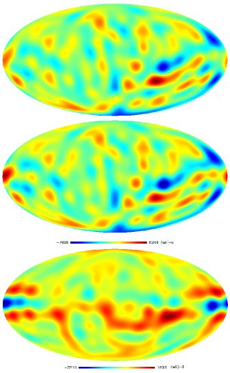
Figure 1: Top: A bipolar map generated from bipolar coefficients, $A_{\ell M}$, of 3-year ILC map. Middle: bipolar map based on 1-year ILC map and Bottom: differences between the two maps (note the scales). The top map (ILC-3) has smaller fluctuations comparing to the middle one (ILC-1) except for the hot spot near the equator. Differences between these two maps mostly arise from a band around the equator in bipolar space. Both ILC maps are smoothed by a band pass filter, $W^{S}(l_{t}=2,l_{s}=10)$.

IV.1 First Method: BiPS

Among the several possible combinations of BipoSH coefficients, the Bipolar Power Spectrum (BiPS) was proved to be a useful tool with interesting features Hajian & Souradeep (2003b). BiPS of CMB anisotropy is defined as a convenient contraction of the BipoSH coefficients

$$\kappa_{\ell}\,=\,\sum_{l,l^{\prime},M}\left|A_{\ell M|ll^{\prime}}\right|^{2}\geq 0.$$ (13)

BiPS is interesting because it is orientation independent, i.e. invariant under rotations of the sky. For models in which statistical isotropy is valid, BipoSH coefficients are given by eqn (11), and therefore SI condition implies a null BiPS, i.e. $\kappa_{\ell}\,=\,0$ for every $\ell>0$,

$$\kappa_{\ell}\,=\,\kappa_{0}\delta_{\ell 0}.$$ (14)

Non-zero components of BiPS imply break down of statistical isotropy, and this introduces BiPS as a measure of statistical isotropy. It is worth noting that although BiPS is quartic in $a_{lm}$, it is designed to detect SI violation and not non-Gaussianity Hajian & Souradeep (2005, 2003b); Souradeep & Hajian (2004, 2004b); Hajian et al. (2004). An un-biased estimator of BiPS is given by

$$\tilde{\kappa}_{\ell}=\sum_{ll^{\prime}M}\left|A_{\ell M|ll^{\prime}}\right|^{2}-{\mathfrak{B}}_{\ell}\,,$$ (15)

where ${\mathfrak{B}}_{\ell}$ is the bias that arises from the SI part of the map and is given by the angular power spectrum, $C_{l}$,

$${\mathfrak{B}}_{\ell} \equiv \langle\tilde{\kappa}_{\ell}^{B}\rangle_{{}_{\rm SI}}$$

$$= (2\ell+1)\,\sum_{l_{1}}\sum_{l_{2}=|\ell-l_{1}|}^{\ell+l_{1}}W_{l_{1}}W_{l_{2}}\times$$

$$\,\,\,\,\,\,\,\,\,\,\,\,\,\,\,\,\,\,\,\,\left[C_{l_{1}}C_{l_{2}}+(-1)^{\ell}\,\delta_{l_{1}l_{2}}\left(C_{l_{1}}\right)^{2}\right]\,.$$

The above expression for ${\mathfrak{B}}_{\ell}$ is obtained by assuming Gaussian statistics of the temperature fluctuations Hajian & Souradeep (2003b, 2005).

IV.2 New Method: Reduced Bipolar Coefficients

The BipoSH coefficients of eqn. (12) can be summed over $l$ and $l^{\prime}$ to reduce the cosmic variance,

$$A_{\ell M}=\sum_{l=0}^{\infty}\sum_{l^{\prime}=|\ell-l|}^{\ell+l}A_{\ell M|ll^{\prime}}.$$ (17)

These reduced bipolar coefficients, $A_{\ell M}$, by definition respect the following symmetry:

$$A_{\ell M}=(-1)^{M}A_{\ell-M}^{*},$$ (18)

which indicates $A_{\ell 0}$ are always real. When SI condition is valid, the ensemble average of $A_{\ell M}$ vanishes for all $\ell$ and $M$

$$\langle A_{\ell M}\rangle=0.$$ (19)

In any given CMB anisotropy map, $A_{\ell M}$ would fluctuate about zero. A severe breakdown of statistical isotropy will result in huge deviations from zero. Reduced bipolar coefficients are not rotationally invariant, hence they assign direction to the correlation patterns of a map. We can combine $A_{\ell M}$ further to define a power spectrum similar to how $a_{lm}$ are combined to construct the angular power spectrum, $C_{l}$. We define

$$D_{\ell}=\frac{1}{2\ell+1}\sum_{M=-\ell}^{\ell}A_{\ell M}A_{\ell M}^{*}.$$ (20)

The above estimator is rotationally invariant. It has a positive bias and hence it has similar issues that have been addressed for the BiPS studies earlier. This means although the ensemble average of $A_{\ell M}$ for a statistically isotropic case is zero, ensemble average of $D_{\ell}$ is always greater than zero. However a major deviation from statistical isotropy will result in a big $D_{\ell}$ (compared to that of a SI case). In section V we compare $A_{\ell M}$ of ILC map against an average of 1000 simulations of statistically isotropic maps. We defer detailed studies of $D_{\ell}$ to the future publication.

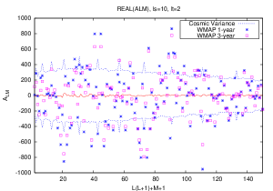
Figure 2: Real part of $A_{\ell M}$’s of ILC-3 (red square points) and ILC-1 (blue stars) for a $W^{S}(10,2)$ filter that roughly keeps multipoles between 2 and 15. $\ell$ and $M$ indices are combined to a single index $n=\ell(\ell+1)+M+1$ and the blue dotted lines define 1-$\sigma$ error bars derived from 1000 simulations of SI CMB anisotropy maps. Almost all of $A_{\ell M}$’s of ILC-3 are smaller than those of ILC-1 which means ILC-3 is more consistent with statistical isotropy.

V Application to the WMAP Data

We carry out our analysis on 3-year ILC map and compare it to 1-year ILC map. In order to attribute a statistical significance to our results, we compare our results to 1000 simulations of SI CMB maps. $a_{lm}$’s of these maps are generated up to an $l_{max}$ of 1024 (corresponding to HEALPix resolution $N_{side}=512$). Since we are only interested in large angular scales we smooth all maps with appropriate filters to cut the power on small angular scales. These filters are low pass Gaussian filters

$$W_{l}^{G}=N^{G}\exp\left\{-\left(\frac{2l+1}{2l_{s}+1}\right)^{2}\right\}$$ (21)

that cut power on scales $(l\geq l_{s})$ and band pass filters of the form

$$W_{l}^{S}=2N^{S}\left[1-J_{0}\left(\frac{2l+1}{2l_{t}+1}\right)\right]\exp\left\{-\left(\frac{2l+1}{2l_{s}+1}\right)^{2}\right\},$$ (22)

that keep the power on scales corresponding to $l_{t}<l<l_{s}$.$J_{0}$ is the bessel function and $N^{G}$ and $N^{S}$ are normalization constants chosen such that,

$$\sum_{l}\frac{(2l+1)W_{l}}{2l(l+1)}=1$$ (23)

i.e., unit rms for unit flat band angular power spectrum $C_{l}=\frac{2\pi}{l(l+1)}$.

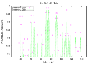
Figure 3: Fraction of $A_{\ell M}$’s in 1000 simulations that are smaller than $A_{\ell M}$’s of ILC. Several deviations in ILC-1 (red square points) have been corrected in ILC-3 (green impulses). Only deviations above 68% are shown. Almost all of $A_{\ell M}$’s of ILC-3 are smaller than those of ILC-1 which means ILC-3 is more consistent with statistical isotropy. Only real parts are shown. Points are always in pairs because of the symmetry in reduced bipolar coefficients, $A_{\ell M}=(-1)^{M}A_{\ell-M}^{*}$. All maps are smoothed with a $W^{S}(10,2)$ filter.

We compute the BipoSH coefficients, $A_{\ell M|ll^{\prime}}$, for 3-year ILC map (ILC-3) for several window functions using eqn. (12). We combine these coefficients using eqn. (17) to obtain $A_{\ell M}$. An interesting way of visualizing these coefficients is to make a map from them. Making a map from $A_{\ell M}$ is simply done similar to making a temperaure anisotropy map from a given set of spherical harmonic coefficients, $a_{lm}$;

$$\Theta(\hat{n})=\sum_{\ell=0}^{\infty}\sum_{M=-\ell}^{\ell}A_{\ell M}Y_{\ell M}(\hat{n}).$$ (24)

The symmetry of reduced bipolar coefficients, eqn. (18), guarantees reality of $\Theta(\hat{n})$. The “bipolar” map based on bipolar coefficients of ILC-3 is shown on the top panel of Fig. 1. The map has small fluctuations except for a pair of hot and cold spots near the equator. To compare, we have also made a bipolar map of 1-year ILC map (ILC-1) from bipolar coefficients of ILC-1 (middle panel of Fig. 1). The difference map (Fig. 1 (bottom)) shows that differences between these two maps mostly arise from a band around the equator in bipolar space. As it is seen in Fig. 1, the bipolar map of ILC-3 has less fluctuations comparing to that of ILC-1. This is because almost all of $A_{\ell M}$’s of ILC-3 are smaller than those of ILC-1 (i.e. are closer to zero). Reduced bipolar coefficients of the above maps are in Figure 2, in which $\ell$ and $M$ indices are combined to a single index $n=\ell(\ell+1)+M+1$ (only real part of $A_{\ell M}$ is plotted.). And the blue dotted lines define 1-$\sigma$ error bars derived from 1000 simulations of SI CMB anisotropy maps. As it can be seen many spikes presented in $A_{\ell M}$’s of ILC-1 have either disappeared or reduced in ILC-3 (e.g. those around $n=20,40$ and a big spike at $n=111$). To get a quantitative description of differences between ILC-3 and ILC-1 we compare them against 1000 simulations of SI CMB anisotropy maps. A simple $\chi^{2}$ comparison of $A_{\ell M}$ with simulations gives us a rough estimate of overall differences between the two ILC maps: ILC-3 has a smaller $\chi^{2}$ than ILC-1. For a $W^{S}(10,2)$ filter, the reduced $\chi^{2}$ falls from $1.089$ for ILC-1 to $0.9619$ for ILC-3. Although $\chi^{2}$ statistics is simple, it should be used with caution because it is only valid if every $A_{\ell M}$ is independent has a Gaussian distribution function. In order to study deviations of $A_{\ell M}$ from zero without worrying about the Gaussianity of the $A_{\ell M}$, we look at the most deviant (biggest) $A_{\ell M}$. We compare the biggest $A_{\ell M}$’s of ILC to $A_{\ell M}$’s of 1000 simulations to find out what fraction of simulations have $A_{\ell M}$’s smaller than those of ILC maps. Figure 3 shows the results. The horizontal axis is $n=\ell(\ell+1)+M+1$ and the vertical axis is the fraction of $A_{\ell M}$’s in 1000 simulations that are smaller than $A_{\ell M}$ of ILC. In this figure red squares represent the ILC-1 while ILC-3 is represented by green lines. When a green line crosses a red point, $A_{\ell M}$’s of ILC-3 are greater than ILC-1, otherwise red points above green spikes show smaller $A_{\ell M}$’s for ILC-3. The results are interesting: several deviations in ILC-1 have been corrected in ILC-3. Specially on the largest scales, several deviations beyound $95\%$ in ILC-1 have gone away in ILC-3 (red points above the blue dotted line in Figure 3 have been replaced by significantly smaller values). However there are a couple of exceptions that could be responsible for the hotter spot in bipolar map of ILC-3.

Combining the BipoSH coefficients to construct bipolar power spectrum allows further examinations of ILC maps for departures from SI. We compute the BiPS using eqn. (15). It is worth mentioning that BiPS in this paper has been computed in a slightly different way than in our previous paper Hajian et al. (2004). Here we compute the BiPS using eqn. (15) and we use the derived $C_{l}$ from each map to estimate the bias, ${\mathfrak{B}}_{\ell}$, using eqn. (IV.1). The bias corrected BiPS is then averaged over 1000 simulations and is compared to bias corrected BiPS of ILC maps. BiPS results shown in Figure 4 agree with our results on $A_{\ell M}$. It can be seen that ILC-3 has a smaller bipolar power spectrum than ILC-1 and is more consistent with statistical isotropy. The same is true for $D_{\ell}$ estimator defined by eqn. (20) which we defer to the future publications. We should emphasize that these results are only for large angular scales, $l\leq 25$, and not beyond that.

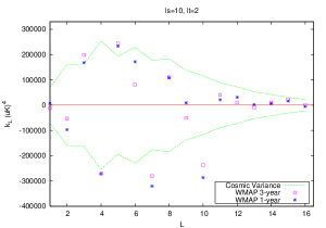
Figure 4: Bipolar power spectrum (BiPS) of the two ILC maps compared to average BiPS of 1000 simulations of statistically isotropic CMB maps. Both ILC maps are smoothed with a $W^{S}(10,2)$ window function which roughly retains multipoles in the range of $2\leq l\leq 15$. ILC-3 shows smaller BiPS than ILC-1, which means it is more consistent with statistical isotropy. Filtering the data with other functions show almost the same results.

VI Discussion and Conclusions

The null results of search for departure from statistical isotropy has implications for the observation and data analysis techniques used to create the CMB anisotropy maps. Observational artifacts such as non-circular beam, inhomogeneous noise correlation, residual striping patterns, and residuals from foregrounds are potential sources of SI breakdown. Our null results confirm that these artifacts do not significantly contribute to large scale anisotropies of 3-year ILC map. We have also quantified the differences between 1-year and 3-year ILC maps. It is shown that 3-year ILC map is “cleaner” than 1-year ILC map at $l\leq 25$. This can be due to the gain model and improved ILC map processing and foreground minimization. It has also been observed that at large $l$ deviations from statistical isotropy occur which we think is because of residuals from foregrounds. However we limit ourselves to the low-$l$ limit because in addition to observational artifacts, there are theoretical motivations for hunting for SI violation on large scales of CMB anisotropy. Topologically compact spaces Ellis (1971); Lachieze-Rey & Luminet (1995); Levin (2002); Linde (2004) and anisotropic cosmological models Ellis & MacCallum (1969); Collins & Hawking (1973a, b); Doroshkevich et al. (1975); Barrow et al. (1985); Jaffe et al. (2006); Ghosh et al. (2006) are examples of this. Each of these models will cause departures from statistical isotropy in CMB anisotropy maps. And a null detection of departure from statistical isotropy at low $l$ in the WMAP data can be used to put constraints on these models. Our measure is sensitive to axial asymmetries in the two point correlation of the temperature anisotropy Hajian & Souradeep (2003a). And this is even more significant now because the new measure of reduced bipolar coefficients does retain directional information. Our analysis doesn’t show a significant detection of an “axis of evil” in the WMAP data. We have redone our analysis on ILC map filtered with a low-pass filter that only keeps $l=2,3,4$ to search for a preferred direction at low multipoles. We have not been able to detect any significant deviation from statistical isotropy using various filters. We could not test the effect of alignment of low multipoles on statistical isotropy because we had no theory or model to explain them. Validity of statistical isotropy at large angular scales can put tight constraints on anisotropic mechanisms that are candidates of explaining the low quadrupole of the WMAP and COBE data. It is worth noticing that our method can be extended to polarization maps of CMB anisotropy. Analysis of statistical isotropy of full-sky polarization maps of WMAP are currently under progress and will be reported in a separate publication.

VII Summary

We examine statistical isotropy of large scale anisotropies of the improved Internal Linear Combination (ILC) map, based on three year WMAP data. In order to attribute a statistical significance to our results, we use 1000 simulations of statistically isotropic CMB maps. We have done our analysis using a series of filters that span the low-$l$ multipoles. We only explicitly present the results for one of them that roughly retains power in the multipoles between 2 and 15. This reveals no significant deviation from statistical isotropy on large angular scales of 3-year ILC map. Comparing statistical isotropy of 3-year ILC map and 1-year ILC map, we find a significant improvement in 3-year ILC map which can be due to the gain model and improved ILC map processing and foreground minimization. We get consistent and similar results from other filters.

Appendix A Useful mathematical relations

Bipolar spherical harmonics form an orthonormal basis of $S^{2}\times S^{2}$ and are defined as

$$Y^{l_{1}l_{2}}_{\ell M}(\hat{n}_{1},\,\hat{n}_{2})\,=\,\sum_{m_{1}m_{2}}{\mathcal{C}}_{l_{1}m_{1}l_{2}m_{2}}^{\ell M}Y_{l_{1}m_{1}}(\hat{n}_{1})Y_{l_{2}m_{2}}(\hat{n}_{2}),$$ (25)

in which ${\mathcal{C}}_{l_{1}m_{1}l_{2}m_{2}}^{\ell M}$ are Clebsch-Gordan coefficients. Clebsch-Gordan coefficients are non-zero only if triangularity relation holds, $\{l_{1}l_{2}\ell\}$, and $M=m_{1}+m_{2}$. Where the $3j$-symbol $\{abc\}$ is defined by

$$\{abc\}=\left\{\begin{array}[]{ll}1&\textrm{if $a+b+c$ is integer and $|a-b|\leq c\leq(a+b)$,}\\ 0&\textrm{otherwise,}\end{array}\right.$$

Orthonormality of bipolar spherical harmonics

$$\int d\Omega_{\hat{n}_{1}}d\Omega_{\hat{n}_{2}}\,Y^{l_{1}l_{2}}_{\ell M}(\hat{n}_{1},\,\hat{n}_{2})Y^{*l^{\prime}_{1}l^{\prime}_{2}}_{\ell^{\prime}M^{\prime}}(\hat{n}_{1},\,\hat{n}_{2})=\delta_{l_{1}l^{\prime}_{1}}\delta_{l_{2}l^{\prime}_{2}}\delta_{\ell\ell^{\prime}}\delta_{MM^{\prime}}$$ (26)

References

- Eriksen et al. (2004a) H. K. Eriksen, F. K. Hansen, A. J. Banday, K. M. Gorski and P. B. Lilje, Astrophys. J. 605, 14 (2004) [Erratum-ibid. 609, 1198 (2004)] [arXiv:astro-ph/0307507].
- Copi et al. (2004) C. J. Copi, D. Huterer and G. D. Starkman, Phys. Rev. D 70, 043515 (2004) [arXiv:astro-ph/0310511].
- Schwarz et al. (2004) D. J. Schwarz, G. D. Starkman, D. Huterer and C. J. Copi, Phys. Rev. Lett. 93, 221301 (2004) [arXiv:astro-ph/0403353].
- Hansen et al. (2004) F. K. Hansen, A. J. Banday and K. M. Gorski, arXiv:astro-ph/0404206.
- de Oliveira-Costa et al. (2003) A. de Oliveira-Costa, M. Tegmark, M. Zaldarriaga, & A. Hamilton, 2004, Phys. Rev.D69, 063516.
- Land & Magueijo (2005a) K. Land and J. Magueijo, Mon. Not. Roy. Astron. Soc. 357, 994 (2005) [arXiv:astro-ph/0405519].
- Land & Magueijo (2005b) K. Land and J. Magueijo, Phys. Rev. Lett. 95, 071301 (2005) [arXiv:astro-ph/0502237].
- Land & Magueijo (2005c) K. Land and J. Magueijo, Mon. Not. Roy. Astron. Soc. 362, 838 (2005) [arXiv:astro-ph/0502574].
- Land & Magueijo (2005d) K. Land and J. Magueijo, Phys. Rev. D 72, 101302 (2005) [arXiv:astro-ph/0507289].
- Land & Magueijo (2005e) K. Land and J. Magueijo, arXiv:astro-ph/0509752.
- Bielewicz et al. (2004) P. Bielewicz, K. M. Gorski and A. J. Banday, Mon. Not. Roy. Astron. Soc. 355, 1283 (2004) [arXiv:astro-ph/0405007].
- Bielewicz et al. (2005) P. Bielewicz, H. K. Eriksen, A. J. Banday, K. M. Gorski and P. B. Lilje, Astrophys. J. 635, 750 (2005) [arXiv:astro-ph/0507186].
- Copi et al. (2006) C. J. Copi, D. Huterer, D. J. Schwarz and G. D. Starkman, Mon. Not. Roy. Astron. Soc. 367, 79 (2006) [arXiv:astro-ph/0508047].
- Copi et al. (2006b) C. Copi, D. Huterer, D. Schwarz and G. Starkman, arXiv:astro-ph/0605135.
- Naselsky et al. (2004) P. D. Naselsky, L. Y. Chiang, P. Olesen and O. V. Verkhodanov, Astrophys. J. 615, 45 (2004) [arXiv:astro-ph/0405181].
- Prunet et al. (2005) S. Prunet, J. P. Uzan, F. Bernardeau and T. Brunier, Phys. Rev. D 71, 083508 (2005) [arXiv:astro-ph/0406364].
- Gluck & Pisano (2005) M. Gluck and C. Pisano, arXiv:astro-ph/0503442.
- Stannard & Coles (2005) A. Stannard and P. Coles, Mon. Not. Roy. Astron. Soc. 364, 929 (2005) [arXiv:astro-ph/0410633].
- Bernui et al. (2005) A. Bernui, B. Mota, M. J. Reboucas and R. Tavakol, arXiv:astro-ph/0511666.
- Bernui et al. (2006) A. Bernui, T. Villela, C. A. Wuensche, R. Leonardi and I. Ferreira, arXiv:astro-ph/0601593.
- Movahed et al. (2006) M. Sadegh Movahed, F. Ghasemi, S. Rahvar and M. Reza Rahimi Tabar, arXiv:astro-ph/0602461.
- Freeman et al. (2006) P. E. Freeman, C. R. Genovese, C. J. Miller, R. C. Nichol and L. Wasserman, Astrophys. J. 638, 1 (2006) [arXiv:astro-ph/0510406].
- Chen & Szapudi (2005) G. Chen and I. Szapudi, Astrophys. J. 635, 743 (2005) [arXiv:astro-ph/0508316].
- Hajian et al. (2004) A. Hajian, T. Souradeep & N. Cornish, 2005, ApJ 618, L63.
- Hajian & Souradeep (2005) A. Hajian & T. Souradeep, 2005, preprint. (astro-ph/0501001).
- Hinshaw et al. (2006) G. Hinshaw et al., arXiv:astro-ph/0603451.
- (27) N. Jarosik et al., “Three-year Wilkinson Microwave Anisotropy Probe (WMAP) observations: Beam profiles, data processing, radiometer characterization and systematic error limits,” arXiv:astro-ph/0603452.
- (28) L. Page et al., “Three year Wilkinson Microwave Anisotropy Probe (WMAP) observations: Polarization analysis,” arXiv:astro-ph/0603450.
- (29) D. N. Spergel et al., “Wilkinson Microwave Anisotropy Probe (WMAP) three year results: Implications for cosmology,” arXiv:astro-ph/0603449.
- Ellis & MacCallum (1969) G. F. R. Ellis and M. A. H. MacCallum, 1969, Commun. math Phys., 12, 108.
- Collins & Hawking (1973a) C. B. Collins and S. W. Hawking, 1973, Astrophys. J. 180, 317.
- Collins & Hawking (1973b) C. B. Collins and S. W. Hawking, 1973, Mon. Not. R. astr. Soc. 162, 307.
- Doroshkevich et al. (1975) A. G. Doroshkevich, V. N. Lukash and I. D. Novikov, 1975, Soviet Astr., 18, 554.
- Barrow et al. (1985) J. D. Barrow, R. Juszkiewicz and D. H. Sonoda, 1985, Mon. Not. R. astr. Soc., 213, 917.
- Jaffe et al. (2006) T. R. Jaffe, A. J. Banday, H. K. Eriksen, K. M. Gorski and F. K. Hansen, arXiv:astro-ph/0603844.
- Ghosh et al. (2006) T. Ghosh, A. Hajian and T. Souradeep, arXiv:astro-ph/0604279.
- Hajian & Souradeep (2003a) A. Hajian & T. Souradeep, 2003a preprint (astro-ph/0301590).
- Hajian (2006) A. Hajian, PhD Thesis, 2006.
- Saha et al. (2006) R. Saha, A. Hajian, T. Souradeep and P. Jain, 2006, in preparation.
- Bartolo et al. (2004) N. Bartolo, E. Komatsu, S. Matarrese and A. Riotto, Phys. Rept. 402, 103 (2004).
- Komatsu et al. (2003) E. Komatsu et al., Astrophys. J. Suppl. 148, 119 (2003).
- (42) D. A. Varshalovich, A. N. Moskalev and V. K. Kher- sonskii, 1988 Quantum Theory of Angular Momentum (World Scientific).
- Hajian & Souradeep (2003b) A. Hajian & T. Souradeep, 2003b, ApJ 597, L5 (2003).
- Souradeep & Hajian (2004) T. Souradeep and A. Hajian, Pramana 62 (2004) 793-796
- Souradeep & Hajian (2004b) T. Souradeep and A. Hajian, Proceedings of JGRG-14, (2004)
- Ellis (1971) G. F. R. Ellis, 1971, Gen. Rel. Grav. 2, 7.
- Lachieze-Rey & Luminet (1995) M. Lachieze-Rey and J. P. Luminet, Phys. Rept. 254, 135 (1995) [arXiv:gr-qc/9605010].
- Levin (2002) J. Levin, Phys. Rept. 365, 251 (2002) [arXiv:gr-qc/0108043].
- Linde (2004) A. Linde, JCAP 0410, 004 (2004) [arXiv:hep-th/0408164].