The ATESP 5 GHz radio survey

Abstract

Context. The nature and evolutionary properties of the faint radio population, responsible for the steepening observed in the 1.4 GHz source counts below 1 milliJy, are not yet entirely clear. Radio spectral indices may help to constrain the origin of the radio emission in such faint radio sources and may be fundamental in understanding eventual links to the optical light.

Aims. We study the spectral index behaviour of sources that were found in the 1.4 GHz ATESP survey (Prandoni et al. 2000a,b), considering that the ATESP is one of the most extensive sub-mJy surveys existing at present.

Methods. Using the Australia Telescope Compact Array we observed at 5 GHz part of the region covered by the sub-mJy ATESP survey. In particular we imaged a one square degree area for which deep optical imaging in UBVRIJK is available. In this paper we present the 5 GHz survey and source catalogue, we derive the 5 GHz source counts and we discuss the $1.4-5$ GHz spectral index properties of the ATESP sources. The analysis of the optical properties of the sample will be the subject of a following paper.

Results. The 5 GHz survey has produced a catalogue of 111 radio sources, complete down to a ($6\sigma$) limit $S_{lim}(5\;\mbox{GHz})\sim 0.4$ mJy. We take advantage of the better spatial resolution at 5 GHz ($\sim 2\arcsec$ compared to $\sim 8\arcsec$ at 1.4 GHz) to infer radio source structures and sizes. The 5 GHz source counts derived by the present sample are consistent with those reported in the literature, but improve significantly the statistics in the flux range $0.4\la S_{5\;\rm{GHz}}\la 1$ mJy. The ATESP sources show a flattening of the $1.4-5$ GHz spectral index with decreasing flux density, which is particularly significant for the 5 GHz selected sample. Such a flattening confirms previous results coming from smaller samples and is consistent with a flattening of the 5 GHz source counts occurring at fluxes $\la 0.5$ mJy.

1 Introduction

One of the most debated issues about the sub-milliJy radio sources, responsible for the steepening of the 1.4 GHz source counts (Condon 1984, Windhorst et al. 1990), is the origin of their radio emission. Understanding whether the dominant triggering process is star formation or nuclear activity has important implications on the study of the star formation/black hole accretion history with radio-selected samples.

However, despite the extensive work done in the last decade, the nature and the evolutionary properties of the faint radio population are not yet entirely clear. Today we know that the sub-mJy population is a mixture of different classes of objects (low-luminosity/high-z AGNs, star-forming galaxies, normal elliptical and spiral galaxies), with star-forming galaxies dominating the microJy ($\mu$Jy) population (see e.g. Richards et al. 1999), and early–type galaxies and AGNs being more important at sub–mJy and mJy fluxes (Gruppioni et al. 1999; Georgakakis et al. 1999; Magliocchetti et al. 2000; Prandoni et al. 2001b). On the other hand, the relative fractions of the different types of objects are still quite uncertain, and very little is known about the role played by the cosmological evolution of the different classes of objects. Conclusions about the faint radio population are, in fact, limited by the incompleteness of optical identification and spectroscopy, since faint radio sources have usually very faint optical counterparts. Clearly very deep ($R>25$) optical follow-up for reasonably large deep radio samples are critical if we want to probe such radio source populations.

Also important may be multi-frequency radio observations: radio spectral indices may help to constrain the origin of the radio emission in the faint radio sources and may actually be fundamental for understanding eventual links to the optical light. This is especially true if high resolution radio data are available and source structures can be inferred.

Multi–frequency radio data are available only for a few very small ($\la 60$ sources) sub–mJy samples. Such studies indicate that most mJy radio sources are of the steep–spectrum type ($\alpha<-0.5$, assuming $S\sim\nu^{\alpha}$), with evidence for flattening of the spectra at lower flux densities (Donnelly et al. 1987; Gruppioni et al. 1997; Ciliegi et al. 2003). This flattening is consistent with the presence of many flat ($\alpha>-0.5$) and/or inverted ($\alpha>0$) spectral index sources at $\mu$Jy flux densities (Fomalont et al. 1991; Windhorst et al 1993). On the other hand, there is still disagreement about the interpretation of such results.

In the $\mu$Jy population studied by Windhorst et al. (1993) 50% of the sources have intrinsic angular size $\Theta\geq 2.6\pm 1.4$ arcsec, corresponding to $\simeq 5-40$ kpc at the expected median redshift of the sources. Extended (kpc–scale) steep–spectrum radio sources suggest synchrotron emission in galactic disks, while extended flat–spectrum sources may indicate thermal bremsstrahlung from large scale star–formation both occasionally with opaque radio cores. On the other hand, Donnelly et al. (1987) claim that most of the sub–mJy blue radio galaxies have steep radio spectra and are physically quite compact ($\leq 4$ kpc). This suggests two possible alternative mechanisms for the radio emission: 1) a nuclear starburst occurring on a few kpc scale in the galaxy center; 2) a non-thermal nucleus on parsec scales. Only high resolution radio observations could decide between them.

With the aim of studying the spectral index behaviour of the faint radio population, we imaged at 5 GHz a one square degree area of the ATESP 1.4 GHz survey ($S_{\rm lim}\sim 0.5$ mJy, Prandoni et al. 2000a,b), for which deep ($R<25.5$) optical multi-color data is available, as part of an ESO public survey (e.g. Mignano et al. 2006). Such deep optical imaging will provide optical identification and photometric redshifts for most of the radio sources.

We notice that the ATESP is best suited to study the sources populating the flux interval $0.5-1$ mJy, where starburst galaxies start to enter the counts, but are not yet the dominant population. This means that our sample can be especially useful to study the issue of low-luminosity nuclear activity, possibly related to low efficiency accretion processes and/or radio-intermediate/quiet QSOs.

The present 5 GHz observations are valuable because i) the higher resolution images probe the radio source structure at small scales ($\leq 2$ arcsec) and thus we can hopefully distinguish between disk–scale and nuclear–scale radio emission, and ii) the present 5 GHz survey is the largest at sub–mJy fluxes, by a factor $10-100$: previous samples typically cover from $<0.01$ to $\sim 0.1$ square degrees (e.g. Bennett et al. 1983; Fomalont et al. 1984, 1991; Donnelly et al. 1987; Partridge et al. 1986; Ciliegi et al. 2003).

In this paper we describe the ATESP 5 GHz survey, present the 5 GHz source catalogue and counts, and discuss the spectral index properties of the ATESP radio sources. The analysis of the optical properties of the sample will be the subject of a following paper (Mignano et al. in preparation).

The paper is organized as follows. In Sect. 2 we briefly present the 1.4 GHz ATESP survey and the multi-color optical data coming from the ESO Deep Public Survey (DPS). Sect. 3 describes the ATESP 5 GHz survey observations and data reduction. The radio mosaics we produced are discussed in Sect. 4, while Sect. 5 describes the source extraction and parameterization procedure. The 5 GHz source catalogue is presented in Sect 6, together with an analysis of the source size and structure. The 5 GHz source counts derived from the present survey and the $1.4-5$ GHz spectral index properties of the ATESP sources are presented in Sect. 7. A summary is given in Sect. 8.

2 The 1.4 GHz ATESP Survey and Related Optical Information

Figure 1: Sketch of the sky coverage of the radio (ATESP at 1.4 and 5 GHz) and optical (ESP, EIS, DPS) surveys relevant for this study. See text for details.

The ATESP 1.4 GHz survey (Prandoni et al. 2000a ) was carried out with the Australia Telescope Compact Array (ATCA); it consists of 16 mosaics with $8\arcsec\times 14\arcsec$ resolution and uniform sensitivity ($1\sigma$ noise level $\sim 79$ $\mu$Jy), covering two narrow strips of $21^{\circ}\times 1^{\circ}$ and $5^{\circ}\times 1^{\circ}$ near the SGP, at decl. $-40^{\circ}$. The ATESP 1.4 GHz survey has produced a catalogue of 2967 radio sources, down to a flux limit ($6\sigma$) of $S\sim 0.5$ mJy (Prandoni et al. 2000b ).

In order to alleviate the identification work, the area covered by the ATESP survey was chosen to overlap with the region where Vettolani et al. (Vettolani97 (1997)) made the ESP (ESO Slice Project) redshift survey. They performed a photometric and spectroscopic study of all galaxies down to $b_{J}\sim$ 19.4. The ESP survey yielded 3342 redshifts (Vettolani et al. Vettolani98 (1998)), to a typical depth of $z=0.1$ and a completeness level of 90%.

In the same region lies the ESO Imaging Survey (EIS) Patch A ($\sim 3^{\circ}\times 1^{\circ}$ square degrees, centered at $22^{h}40^{m}$, $-40^{\circ}$), mainly consisting of images in the I-band out of which a galaxy catalogue $95\%$ complete to $I=22.5$ has been extracted (Nonino et al. Nonino99 (1999)). This catalogue allowed us to identify $\sim 57\%$ of the 386 ATESP sources present in that region. A first radio/optical analysis of a magnitude-limited sub-sample of 70 sources was presented by Prandoni et al. (2001b).

More recently, a different strip of $2^{\circ}\times 0.5^{\circ}$ within the ATESP region at $22^{h}50^{m}40^{s}$, $-40^{\circ}13^{\prime}$ was selected for a very deep multi-color ESO public survey: the Deep Public Survey (DPS), which was carried out with the Wide Field Imager (WFI) at the 2.2 m ESO telescope. This one square degree region is covered by 4 WFI fields (referred to as DEEP1a,b,c and d). In this region $UBVRI$ imaging down to very faint magnitudes is available (see Mignano et al. 2006): $U\sim 25$, $B\sim 25.8$, $V\sim 25.2$, $R\sim 25.5$, $I\sim 24$ ($5\sigma$, 2 arcsec aperture magnitudes). In addition, DEEP1a and b have been observed in the infrared with SOFI at NTT down to $K_{AB}\sim 21.3$, while deeper J- and K-band images ($J_{AB}<23.4$ and $K_{AB}<22.7$) have been taken for selected sub-regions (see Olsen et al., 2006)

A sketch of the sky coverage of the surveys described in this section is given in Fig. 1.

3 The Observations

3.1 Observing Strategy

We imaged the entire DEEP1 $2\times 0.5$ degree region at 5 GHz, since it has the best optical coverage. The area was spanned with a radio mosaic consisting of $21\times 6$ pointings (fields) at $6^{\prime}$ spacing, i.e. FWHM/$\sqrt{2}$, where FWHM$=10^{\prime}$ is the full width at half maximum of the primary beam (see Prandoni et al. 2000a ). If we aim at virtually detecting all the 1.4 GHz ATESP sources with radio spectral index $\alpha\geq-0.7$, we need to reach a 5 GHz point source detection limit of $3\sigma\simeq 0.2$ mJy.

Of course, correct spectral index determination can only be made if the 5 and 1.4 GHz beams have the same size, as severe incompleteness would result if the extra resolution at 5 GHz were used. Therefore we produced 5 GHz radio mosaics with the same spatial resolution as for the ATESP 1.4 GHz mosaics. We thus used the Compact Array in the 1.5 km configuration. On the other hand we also requested the 6 km antenna. While we want to extract the source catalogue from the low resolution mosaic, the longer baselines to the 6km antenna were exploited to get additional information on the radio source structure (see Sect. 6.2).

Each field (with $2\times 128$ MHz bandwidth and 10 baselines) was observed for 98 minutes, which results in a final uniform noise level of $\sim 64$ $\mu$Jy. Therefore all $21\times 6=126$ fields could be observed in 18 blocks of 12 hours (allowing also for calibration time). Care was taken to obtain good hour angle coverage, by cycling continually through the individual field during the observing process. Since we wanted to observe the entire region also with the 6 km configuration, an additional 12 hours were used for that purpose.

The observing log is given in Table 1. Note that the use of different 1.5 km arrays is not relevant for the present study. The two 128 MHz bands were set at 4800 and 5056 MHz.

The flux density calibration was performed through observations of the source PKS B1934-638, which is the standard primary calibrator for ATCA observations ($S=5.8$ Jy at $\nu=4800$ MHz as revised by Reynolds Reynolds94 (1994), Baars et al. Baarsetal77 (1977) flux scale). The phase and gain calibration was based on observations of a secondary calibrator (source 2254-367) selected from the ATCA calibrator list.

Table 1: Log of the observations.

Date	$t_{\mathrm{obs}}$	Array
	$h$
13/10/00	$1\times 12$	6A
16/11/00–19/11/00	$3\times 12$	1.5B
13/12/00–20/12/00	$7\times 12$	1.5F
02/08/01–10/08/01	$5\times 12$	1.5A
29/10/01–03/11/01	$4\times 12$	1.5D

Table 2: Main parameters for the 2 low resolution mosaics and average values from the 30 full resolution mosaics.

Mosaica	Fields	Tangent Pointb		Synthesized Beamc		$S_{\mathrm{min}}$	$\sigma_{\mathrm{fit}}$	$<\sigma>$
fld $x$ to $y$	$n\times m$	$R.A.$	$DEC.$	$b_{\mathrm{min}}\times b_{\mathrm{maj}}$ ($\arcsec$)	P.A. ($\degr$)	mJy	$\mu$Jy	$\mu$Jy
fld1to11d	$11\times 6$	22 47 39.57	-40 13 00.0	$7.8\times 12.8$	$+3$	$-0.37$	70.0	$70.1\pm 4.2$
fld10to21e	$12\times 6$	22 52 38.16	-40 13 00.0	$7.9\times 13.0$	$-1$	$-0.33$	65.2	$64.1\pm 3.8$
full res. mosaicsf				$(2.1\times 3.5)\pm(0.1\times 0.2)$	$1\pm 4$	$-0.37\pm 0.13$	$70.1\pm 3.6$	$70.1\pm 4.1$
a $x$ and $y$ refer to the first and last field columns composing the mosaic.
b J2000 reference frame.
c P.A. is defined from North through East.
d Low res. mosaic overlapping the 1.4 GHz ATESP mosaic fld05to11 (see Prandoni et al. 2000a ).
e Low res. mosaic overlapping the 1.4 GHz ATESP mosaic fld10to15 (see Prandoni et al. 2000a ).
f Average values from the 30 full resolution mosaics.

3.2 Data Reduction

For the data reduction we used the Australia Telescope National Facility (ATNF) release of the Multichannel Image Reconstruction, Image Analysis and Display (MIRIAD) software package (Sault et al. Sault95 (1995)).

Every single $12^{\mathrm{h}}$ run and each of the two observing bands were flagged and calibrated following standard procedures for ATCA observations, as described in Prandoni et al. (2000a ).

Sensitivity and $u-v$ coverage were improved for each field by merging, before imaging and cleaning, the visibilities coming from all the observing runs and from the two observing bands. Imaging and deconvolution was done simultaneously for several pointings. This is not only simpler and faster, but also produces better results, as overlapping pointings can make use of a higher number of visibilities and side lobes of sources in contiguous fields can be easlily cleaned.

We produced mosaics at both low and full resolution ($\sim 10\arcsec$ and $\sim 2\arcsec$ respectively). Two low resolution mosaics covered the entire $2\degr\times 0.5\degr$ region, while in full resolution 30 overlapping mosaics of 9 pointings each were produced. Final images were obtained by cleaning after (phase only) self calibration.

Snapshot surveys like the present one are typically affected by the clean bias effect: the deconvolution process can produce a systematic underestimation of the source fluxes, as consequence of the loose constraints to the cleaning algorithm due to sparse $u-v$ coverage (see White et al. White97 (1997); Condon et al. Condonetal98 (1998)). The clean bias effect has been discussed in great detail (Prandoni et al. 2000a ), and we repeat here only that such a systematic effect can be kept under control if cleaning is stopped well before the maximum residual flux has reached the theoretical noise level. Specifically, we set the cleaning limit at 4 times the theoretical noise, since simulations made by us show that this cut-off ensures that the clean bias does not affect source fluxes.

Another systematic effect that has to be taken into account is bandwidth smearing. It is well known that at large distance from the pointing centre bandwidth smearing tends to reduce the peak flux and increase the apparent source size in the radial direction, such that total flux remains conserved. Also this effect has been discussed by us extensively in an earlier paper on the ATESP 1.4 GHz survey (Prandoni et al. 2000b), in particular in the context of radio mosaics. Considering that the passband width is 4 MHz, for the multichannel $32\times 4$ MHz continuum mode observations, and the observing frequency about 5000 MHz, it is easily seen from equation (8) in Prandoni et al. (2000b) that the ratio between smeared and unsmeared peak flux is between 0.9999 and 1. Consequently bandwidth smearing is of no concern for our 5 GHz survey.

4 The Radio Mosaics

4.1 Production of the Mosaics

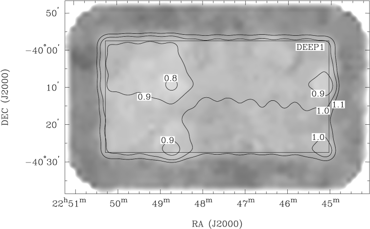
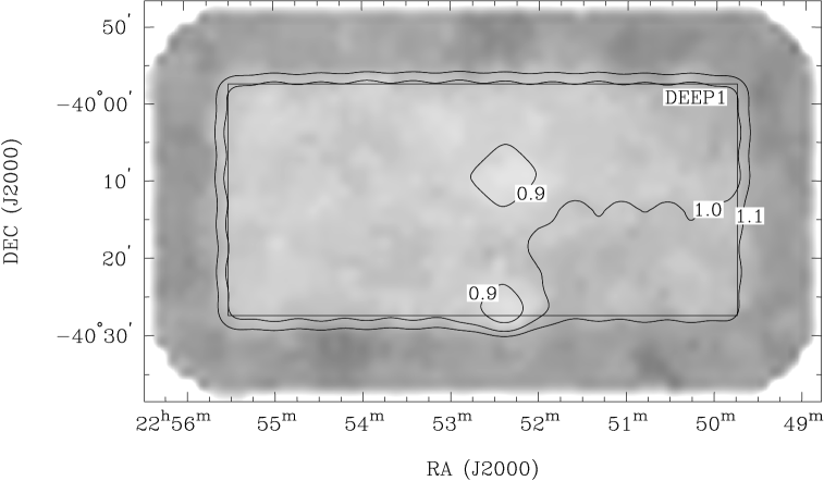
Figure 2: Top: Grey scale of the noise maps obtained from the two low resolution mosaics: fld1to11 (Top) and fld10to21 (Bottom). Darker regions correspond to higher noise. The rectangular boxes indicate the region corresponding to the DEEP1 area, where the survey was designed to provide a uniform noise level. The contour images represent the theoretical sensitivity computed by taking into account the observing time actually spent on the mosaiced single fields: contours refer to 1.1, 1.0, 0.9, 0.8 $\times$ the mean noise value estimated in the noise maps (see Fig. 3). As expected the actual noise variations trace reasonably well the theoretical ones.

As mentioned before, we needed to produce mosaics at exactly the same resolution as the 1.4 GHz images (see Prandoni et al. 2000a ), in order to be able to compare the data at two frequencies and determine reliable spectral indices. We therefore used only the 10 baselines shorter than 3 km. Radio maps with $520\times 520$ pixels of 2.5 arcsec were made, and combined into two mosaics. In this way all the flux in the primary beam (which is 20.6 arcmin at 4800 MHz) is recovered. Details on the two low resolution mosaics (which are of the order of $2000\times 1200$ pixels. and have a small overlap) are given in Table 2: we list the number of fields composing the mosaics (columns $\times$ rows), the tangent point (sky position used for geometry calculations) and the restoring synthesized beam (size in arcsec and position angle).

Since the aim of the low resolution imaging is basically sensitivity, natural weighting was used in the deconvolution process. However, this choice may introduce some spatially correlated features and this may affect the zero level of faint radio sources. This problem can be avoided by removing all baselines shorter than 60 m from the data prior to imaging and deconvolving.

Although this means that $\sim 3-7\%$ of the visibilities in 1.5B and 1.5F configurations had to be rejected, this had hardly any adverse effect on the quality of the mosaics. The lack of the shortest spacings would in principle lead to an increased insensitivity to sources larger than $90\arcsec$, but in reality less than one source with angular size $>90\arcsec$ is expected in the area and flux range covered by the present survey (as discussed in Sect. 6.2). Therefore the effect on completeness and flux densities should be minimal.

In order to assess the radio source structures full resolution images were produced. The $2\times 0.5$ sq. degr. region was covered by a grid of 30 overlapping mosaics, each composed by $3\times 3$ or $3\times 2$ fields. A size of $2060\times 2060$ pixels (with a pixel size of $0.6\arcsec$) for each field in the mosaics ensured complete recovery of the whole flux in the field of the primary beam. Some average parameters of the full resolution mosaics are given in Table 2.

4.2 Noise Analysis of the Mosaics

The 5 GHz survey was designed to give uniform noise in the central $1.0\degr\times 0.5\degr$ regions of the two low resolution mosaics, which together cover the area of the DEEP1 optical survey (see Mignano et al. 2006). In the following our noise analysis always refers to this region. In column 7 of Table 2 we list the minimum (negative) flux $S_{\mathrm{min}}$ found in the image, in column 8 the noise $\sigma_{\mathrm{fit}}$ estimated as the FWHM of the flux distribution in the pixels in the range $\pm S_{\mathrm{min}}$, and in column 9 the noise $<\sigma>$ estimated as the standard deviation of the average flux in several source-free sub-regions of the mosaics. $\sigma_{\mathrm{fit}}$ was used to check the presence of correlated noise, while $<\sigma>$ gives an idea of the uniformity of the noise over the area of the mosaic. As expected, noise variations in general do not exceed $\sim 10\%$, with the sole exception of one of the full resolution mosaics, due to the presence of an $S=27$ mJy source that could not effectively be self-calibrated. On average we find a noise level around $\sim 70$ $\mu$Jy; therefore a $3\sigma$ detection limit for a 5 GHz source at the position of a 1.4 GHz source is $\sim 0.21$ mJy. In all mosaics the noise is essentially Gaussian.

A more detailed analysis of the noise has been performed for the two low resolution mosaics, since they are used for source extraction. The root-mean-square variations of the background were determined with the software package Sextractor (Bertin & Arnouts 1996), which was developed for the analysis of optical images, but is known to work well also on radio images (see Bondi et al. 2003, Huynh et al. 2005).

In computing the local background variations we used a mesh size of $32\times 32$ pixels (or equivalently $8\times 8$ beams) as this was empirically found to be a good compromise: too small mesh sizes would suffer from individual source statistics, while large meshes would miss large. real systematic variations of the background. We remark that a very similar mesh size proved to work well for the ATCA 1.4 GHz survey of the HDF South done by Huynh et al. (2005).

The noise maps for the two low resolution mosaics are shown in Fig. 2 (grey scale). Also shown are the expected theoretical sensitivities due field to field variations in the actual observing time (contours). We notice that the measured noise is quite uniform in the inner part of the mosaics, and traces the expected sensitivity quite well.

In Fig. 3 we plot the pixel flux value distributions in the noise maps. The vertical dotted lines indicate the mean value of the distributions ($68.5\pm 4.4$ $\mu$Jy for fld1to11 and $63.3\pm 4.2$ $\mu$Jy for fld10to21) and the corresponding $\pm 10\%$ variations. We notice that such noise values are in very good agreement with the average noise values obtained directly from the radio mosaics (see Tab. 2). In addition the two distributions in Fig. 3 clearly show that noise variations larger than $10\%$ are very rare. In particular the largest noise values are found in presence of strong radio sources, while the lowest noise values are due to longer observing times on some fields.

The noise maps derived for the two low resolution mosaics have been used to define a local signal to noise ratio, i.e. a local threshold, for the source detection (see Sect. 5).

Figure 3: Pixel flux value distribution in the (inner part of) noise maps. Top: fld1to11. Bottom: fld10to21. The vertical dotted lines indicate the mean value and the corresponding $\pm 10\%$ variations for each map.

5 Source Extraction

As for our 1.4 GHz survey we used the algorithm IMSAD (Image Search and Destroy), available as part of the MIRIAD package for the source extraction and parameterization. The source catalogue thus obtained is based on the low resolution mosaics exclusively.

As a first step, we extracted all sources with peak flux $S_{\rm peak}\geq 4.5\sigma$, where $\sigma=\sigma_{fit}$ is the average mosaic rms flux density (see Table 2). This yielded a preliminary list of 141 source components with $S_{\rm peak}\ga 0.3$ mJy in a total area of $2\times 0.5$ sq. degr.

All the sources were then visually inspected in order to check for obvious failures and/or possibly poor parameterization. Whenever necessary the sources were re-fitted. The checking/re-fitting procedures adopted in this work are the same as used for the compilation of the 1.4 GHz ATESP source catalogue and we refer to Sect. 2 of Prandoni et al. (2000b ) for a full description. In a few cases Gaussian fits were able to provide good values for positions and peak flux densities, but did fail in determining the integrated flux densities. This happens typically at faint fluxes ($<10\sigma$). Gaussian sources with a poor determination of $S_{\rm total}$ are flagged in the catalogue (see Sect. 6.1).

After obtaining reliable parameters for all the sources, we used the noise maps described in Sect. 4.2 to compute the local signal-to-noise ratio for each source. Any source with $S_{peak}\geq 6\sigma_{\rm{local}}$ was then included in the final list: 115 sources (or source components) satisfy this criterion. The peak flux density distribution for the final source sample is shown in Fig. 4.

Fig. 5 shows the so-called visibility area of the ATESP 5 GHz survey, i.e. the fraction of the total area covered by the survey, over which a source with given $S_{peak}$ satisfies the $S_{\rm{peak}}\geq 6\sigma_{\rm{local}}$ criterion. We notice that the visibility area increases quite rapidly with flux and becomes equal to 1 at $S_{\rm peak}\sim 0.5$ mJy.

Figure 4: Peak flux density distribution of the 115 5 GHz radio sources (or source components) with $S_{\rm peak}\geq 6\sigma_{\rm{local}}$.

Figure 5: Visibility area of the ATESP 5 GHz survey. Fraction of the total area over which a source with given measured peak flux density can be detected.

5.1 Multiple and Non-Gaussian Sources

When we search for possible multiple-component sources, we find that the nearest neighbour pair separations are always $d\ga 40\arcsec$, with the exception of four cases, where pair separations are $13.1\arcsec$, $18.3\arcsec$, $18.4\arcsec$ and $20.0\arcsec$ respectively. We decided to catalogue these 4 pairs with $d\la 20\arcsec$ as double sources. We notice that three of them show clear signs of association and are the result of the splitting performed by the source fitting procedure itself. Moreover, they are listed as double sources also in the ATESP 1.4 GHz catalogue (Prandoni et al. 2000b). The fourth pair case ($d=20.0\arcsec$) is less obvious, since no clear signs of association are visible. Nevertheless this object is listed as triple source in the ATESP 1.4 catalogue. The final 5 GHz source list consists then in 111 distinct objects: 107 single sources and 4 double sources.

The position of multiple sources is defined as the radio centroid, i.e. as the flux-weighted average position of all the components. Integrated global source flux densities are computed by summing all the component integrated fluxes. The global source angular size is defined as largest angular size (las) and it is computed as the maximum distance between the source components.

We have also four sources which could not be parametrised by a single or multiple Gaussian fit. Non-Gaussian sources have been parameterized as follows: positions and peak flux densities have been derived by a second-degree interpolation of the flux density distribution. This means that positions refer to peak positions, which, for non-Gaussian sources does not necessarily correspond to the position of the core. Integrated fluxes have been derived directly by summing pixel per pixel the flux density in the source area, defined as the region enclosed by the $\geq 3\sigma$ flux density contour. The source position angle was determined by the direction in which the source is most extended and the source axes were defined again as las, i.e., in this case, the maximum distance between two opposite points belonging to the $3\sigma$ flux density contour along (major axis) and perpendicular to (minor axis) the same direction. These four non-Gaussian sources were catalogued at 1.4 GHz as follows: 2 non-Gaussian sources, 1 double source, 1 single Gaussian source.

5.2 Deconvolution

The ratio of the integrated flux to the peak flux is a direct measure of the extension of a radio source:

$$S_{\rm total}/S_{\rm peak}=\theta_{\rm min}\;\theta_{\rm maj}/b_{\rm min}\;b_{\rm maj}$$ (1)

where $\theta_{\rm min}$ and $\theta_{\rm maj}$ are the source FWHM axes and $b_{\rm min}$ and $b_{\rm maj}$ are the synthesized beam FWHM axes. The flux ratio can therefore be used to discriminate between extended (larger than the beam) and point-like sources.

In Fig. 6 we show the flux ratio as a function of signal-to-noise for the 115 sources (or source components) detected above the $6\sigma_{\rm local}$–threshold. Values for $S_{\rm total}/S_{\rm peak}<1$ are due to the influence of the image noise on the measure of source sizes and therefore of the source integrated fluxes. Following Prandoni et al. (2000b , Sect. 3.1), we have taken into account such errors by considering as unresolved all sources which lie below the curve defined by:

$$S_{\rm total}/S_{\rm peak}<1+\left[\frac{a}{(S_{\rm peak}/\sigma_{\rm local})^{\beta}}\right]$$ (2)

where $a=10$ and $\beta=1.5$ (upper dashed line in Fig. 6). Such curve is obtained by determining the lower envelope of the flux ratio distribution (the curve containing 90% of the $S_{\rm total}<S_{\rm peak}$ sources, see lower dashed line in Fig. 6) and then mirroring it on the $S_{\rm total}>S_{\rm peak}$ side.

From this analysis we found that $\sim 70\%$ of the sources (or source components) have to be considered unresolved (dots in Fig. 6). Deconvolved angular sizes are considered meaningful and given in the catalogue only for extended sources (filled circles in Fig. 6); for unresolved sources, angular sizes are set to zero in the catalogue (see Table 6).

Figure 6: Ratio of the integrated flux $S_{\rm total}$ to the peak one $S_{\rm peak}$ as a function of the source signal-to-noise. The horizontal dotted line indicates the $S_{\rm total}=S_{\rm peak}$ locus. Also shown (dashed lines) are the lower and upper envelopes (ref. Eq. 2) of the flux ratio distribution containing $\sim 90\%$ of the unresolved sources (dots). Filled circles indicate extended sources.

5.3 Source Parameters at full resolution

The sources extracted from the low resolution mosaics and catalogued in Table 6 were then searched for in the full resolution mosaics, in order to get additional information on their radio morphology. The detection threshold was set to $3\times$ the local noise level, as allowed whenever the source position is known a priori. The local noise was evaluated in a $\sim 1\arcmin\times 1\arcmin$ box centered on the source position. Above $3\sigma_{\rm local}$ we detected 109 of the 111 sources catalogued at low resolution.

The source full-resolution parameterization has been performed using similar procedures as used at low resolution. Whenever the source peak flux densities were $\geq 6\sigma_{\rm local}$ we performed a two-dimensional Gaussian fit. The sources were then visually inspected and re-fitted, whenever necessary. We also applied Eq. 2 (with $a=5$, $\beta=1.5$) to separate point sources from extended ones.

The full-resolution parameters for each source are reported in Table 6 (Columns 11-20). For sources detected at $<6\sigma_{\rm local}$ (flagged ’$D$’ in the catalogue) we provide only position and peak flux density. In two cases, where the source is very extended and the structure is well recognized, we list all the parameters. Such cases are flagged ’$DE$’. For the two undetected sources (flagged ’$U$’ in the catalogue) we provide peak flux upper limits only.

We notice that 28 sources that are point-like at low resolution get deconvolved at full resolution, implying physical sizes of $1-3$ arcsec. In 3 additional cases, sources which appear as single at low resolution are split in two components at full resolution. Contour images of these three sources, together with the four sources catalogued as double at low resolution, are shown in Fig. 7.

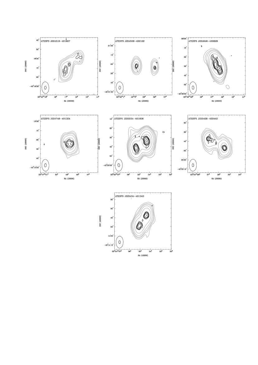
Figure 7: $1\arcmin\times 1\arcmin$ contour images of multiple sources in the catalogue: 7 sources split in two or more components at either low or full resolution. Gray lines are for low resolution contours and black lines are for full resolution contours. For each source the contour levels are at 3, 4.5, 6, 10, 20, 50, 100 $\times$ the local noise level. Synthesized beams at low and full resolution are shown in the lower left corner.

5.4 Errors in the Source Parameters

Parameter uncertainties are the quadratic sum of two independent terms: the calibration errors, which usually dominate at high signal-to-noise ratios, and the internal errors, due to the presence of noise in the maps, which dominate at low signal-to-noise ratios.

For an estimation of the internal errors in the 5 Ghz source parameters we refer to Condon’s master equations (Condon Condon97 (1997)), which provide error estimates for elliptical Gaussian fitting procedures. Such equations already proved to be adequate to describe the measured internal errors for the ATESP 1.4 GHz source parameters (Prandoni et al. 2000b), which have been obtained in a very similar way: same detection algorithm (IMSAD) applied to very similar radio mosaics.

Flux calibration errors are in general estimated from comparison with consistent external data of better accuracy than the one tested. Due to the lack of data of this kind in the region covered by the ATESP 5 GHz survey, we assume the same calibration errors as for the ATESP 1.4 GHz survey, e.g. $5-10\%$ for both flux densities and source sizes (see Appendix A in Prandoni et al. 2000b).

6 The ATESP 5 GHz Sources

6.1 The 5 GHz Source Catalogue

The 5 GHz source catalogue is reported in Table 6. The catalogue is sorted on right ascension. Each source is identified by an IAU name (Column 1) and is defined by its low resolution parameters (Columns $2-10$).

The corresponding full resolution parameters are reported in Columns $11-19$. The detailed format is the following:

Column (1) - Source IAU name. For multiple sources we list all the components (labeled ‘A’, ‘B’, etc.) preceded by a line (flagged ‘M’, see Column 9) giving the position of the radio centroid, the source global flux density and its overall angular size.

Column (2) and (3) - Source position: Right Ascension and Declination (J2000).

Column (4) and (5) - Source peak ($S_{\rm peak}$) and integrated ($S_{\rm total}$) flux densities in mJy (Baars et al. Baarsetal77 (1977) scale).

Column (6) and (7) - Intrinsic (deconvolved from the beam) source angular size. Full width half maximum of the major ($\Theta_{\rm maj}$) and minor ($\Theta_{\rm min}$) axes in arcsec. Zero values refer to unresolved sources (see Sect. 5.2).

Column (8) - Source position angle (P.A., measured N through E) for the major axis in degrees.

Column (9) - Flag indicating the fitting procedure and parameterization adopted for the source (or source component). ‘S’ refers to Gaussian fits; ‘S*’ refers to poor Gaussian fits (see Sect. 5); ‘E’ refers to non-Gaussian sources and ‘M’ refers to multiple sources (see Sect. 5.1).

Column (10) - Local noise level used for the source detection in $\mu$Jy (see Sects. 4.2 and  5).

Columns (11) to (17) - Same as Columns (2) to (8), but referring to full resolution source parameterization.

Column (18) - Same as Column (9), but referring to full resolution source parameterization. Here additional flags are defined for any sources with peak flux $3\sigma_{\rm local}\leq S_{\rm{peak}}<6\sigma_{\rm local}$ and undetected sources (see Sect.5.3). In a few cases references are given to additional notes on full resolution source radio morphology (reported as footnotes at the end of the table).

Column (19) - Same as Column (10) but referring to full resolution mosaics (see Sect. 5.3).

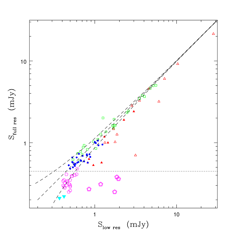
Figure 8: Low resolution vs. full resolution flux densities for the ATESP 5 GHz sample (multiple-component sources are not plotted). We define the flux as $S_{\rm{total}}$ whenever a source is resolved and as $S_{\rm{peak}}$ otherwise. Dashed lines represent the $S_{\rm{full\,res.}}=S_{\rm{low\,res}}$ line and the $1\sigma$ confidence limits in the flux measurements. The horizontal dotted line indicates the average $6\sigma$ detection limit at full resolution. Blue dots: sources appearing point-like at both low and full resolution; green empty squares: sources that are point-like at low resolution, but resolved at full resolution; magenta pentagons: sources point-like at low resolution and detected at $<6\sigma_{\rm{local}}$ at full resolution (flagged ’$D$’ in Column 18 of Table 6); cyan filled triangles (pointing downwards): sources that are point-like at low resolution but undetected at full resolution (flagged ’$U$’ in Column 18 of Table 6); red empty triangles: sources resolved at both low and full resolution; red filled triangles: sources resolved at low resolution and point-like at full resolution; bold magenta pentagons: sources resolved at low resolution and detected at $<6\sigma_{\rm{local}}$ at full resolution (flagged ’$D$’ or ’$DE$’ in Column 18 of Table 6).

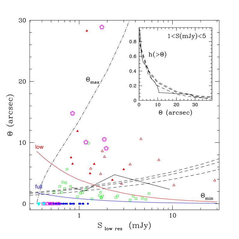
Figure 9: Deconvolved angular size ($\Theta=\Theta_{\rm{maj}}$) as a function of integrated flux density (same sources and symbols as in Fig. 8). We plot low resolution source parameters, except when the source is unresolved at low resolution: in that case we use the full resolution $\Theta_{\rm{maj}}$ estimation. For sources unresolved at both low and full resolution we set $\Theta=0$ and use the peak flux density. The dot-dashed line represents the size ($\Theta_{\rm max}$) above which the ATESP 5 GHz sample gets uncomplete, due to the resolution bias. The two solid lines indicates the minimum angular size ($\Theta_{\rm min}$), below which deconvolution is not considered meaningful at low (red upper line) and at full (blue lower line) resolution respectively. Dashed lines indicate the median source sizes as a function of flux as expected from the Windhorst et al. (1990) relation. Such lines have to be compared to the broken solid line which represents the median source sizes for different flux intervals, as measured in our sample. The inner panel shows the angular size distribution ($h(>\Theta)$ proposed by Windhorst et al. (dashed lines), compared to the size distribution of sources in our sample (broken solid line). See text for more details.

6.2 Source Structure and Size

A comparison between full and low resolution source parameters gives interesting information about the source size and structure.

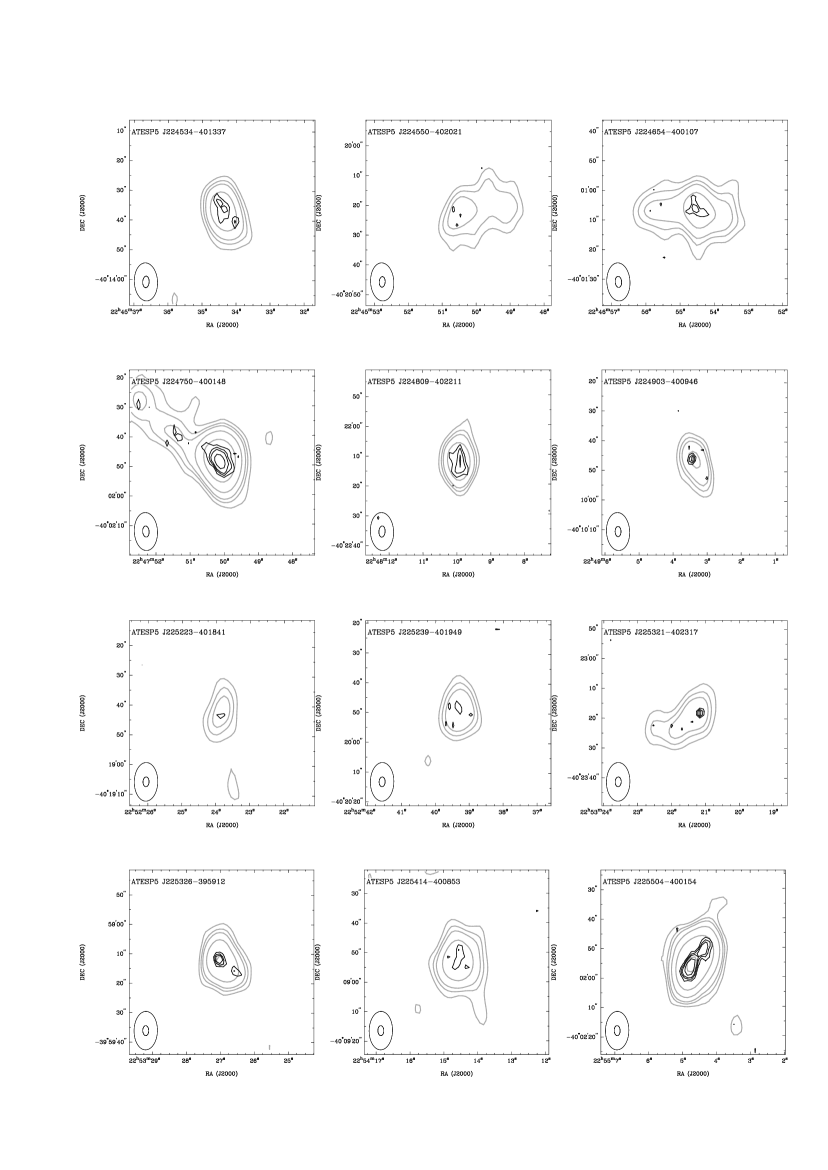
Figure 13: $1\arcmin\times 1\arcmin$ contour images of most extended sources in the catalogue: 12 sources with deconvolved size (at either low or full resolution) larger than $8\arcsec$. Gray lines are for low resolution contours and black lines are for full resolution contours. For each source the contour levels are at 3, 4.5, 6, 10, 20, 50, 100 $\times$ the local noise level. Synthesized beams at low and full resolution are shown in the lower left corner.

In Fig. 8 we compare the flux densities at low and full resolution for the 104 ATESP 5 GHz sources, catalogued as single sources (we exclude the 7 multi–component sources shown in Fig. 7). We find a good correlation between the low and full resolution fluxes, although a number of sources show a systematic integrated flux underestimation at the higher spatial resolution. Such a resolution effect is due to the loss of low surface brightness flux in extended sources, as it is evident from the comparison between Fig. 8 and Fig. 9, where we plot the source deconvolved angular sizes as a function of flux density. In fact the largest sources are typically the ones with largest flux underestimations at full resolution. The most extreme cases regard sources which are resolved at low resolution and are catalogued as point-like (red filled triangles) or even as $<6\sigma_{\rm{local}}$ detections (bold magenta pentagons) at full resolution. In such cases the extended flux gets almost entirely resolved out. We illustrate this effect in Fig. 13, where we show contour images of the 12 most extended single–component sources ($\Theta_{\rm maj}>8\arcsec$). Among such sources there are several cases of low surface brightness sources, which are barely detected at full resolution, and a few cases where full resolution reveals elongated structures and/or hints of multiple components.

The two solid lines in Fig. 9 indicate the minimum angular size, $\Theta_{\rm min}$, below which deconvolution is not considered meaningful at either low (red upper line) or full resolution (blue lower line). They are derived from Eqs. (1) and (2), by setting the appropriate $b_{\rm min}$, $b_{\rm maj}$, $a$ and $\beta$ parameters. We notice that full resolution allows us to get size information for sources with intrinsic sizes ranging from $1-2$ arcsec to $\sim 4$ arcsec (green empty squares). This means that we can successfully deconvolve $\sim 80\%$ of the ATESP 5 GHz sources with $S_{\rm low\,res}>0.7$ mJy and $\sim 90\%$ of the sources with $S_{\rm low\,res}>1$ mJy. Above such flux limits, where we have a limited number of upper limits, we can reliably undertake a statistical analysis of the size properties of our sample. In Fig. 9 we compare the median angular size measured in different flux intervals for the ATESP 5 GHz sources with $S>0.7$ mJy (broken solid line) and the angular size integral distribution derived for the ATESP 5 GHz sources with $1<S(\rm{mJy})<5$ (broken solid line in the inner panel) to the ones obtained from the Windhorst et al. (1990) relations proposed for 1.4 GHz samples: $\Theta_{\rm med}=2\arcsec\cdot S_{1.4\;\rm GHz}^{0.30}$ ($S$ in mJy) and $h(>\Theta)=e^{-ln{2}\;(\Theta/\Theta_{\rm med})^{0.62}}$. $\Theta_{\rm med}$ and $h(>\Theta)$ are extrapolated to 5 GHz using three different values for the spectral index: $\alpha=0$, -0.5 and -0.7 (see black dashed lines). We notice that in the flux ranges considered our determinations show a very good agreement with the ones of Windhorst et al. (1990).

On the other hand, we are not able to say much about the faintest sources ($S<0.7$ mJy), which remain largely unresolved even at full resolution, and constitute about 40% of our sample. We can only argue that the angular sizes of such sources are smaller than $1-2$ arcsec. Such upper limits are consistent with the size analysis performed by Fomalont et al. (1991) for a deeper sample selected at the same frequency (5 GHz): $16/19$ ($84\%$) sources with $0.06<S(\rm{mJy})<0.8$ have $\Theta<1.5$ arcsec. On the other hand, the median values derived from the Windhorst et al. relation (transformed to 5 GHz) might be possibly overestimating the real values (compare black dashed lines to full resolution blue solid line in Fig. 9).

We finally notice that flux losses in extended sources not only affect the full resolution parameterization of the ATESP 5 GHz sources (as shown in Fig. 8), but can also cause incompletess in the ATESP 5 GHz catalogue itself (defined at low resolution). A resolved source of given $S_{\rm total}$ will drop below the peak flux density detection threshold more easily than a point source of same $S_{\rm total}$. This is the so–called resolution bias.

Eq. (1) – with the low resolution parameter setting – can be used to give an approximate estimate of the maximum size ($\Theta_{\rm max}$) a source of given $S_{\rm total}$ can have before dropping below the $S_{\rm peak}=6\sigma_{\rm local}$ limit of the ATESP 5 GHz catalogue. Such limit is represented by the black dot-dashed line plotted in Fig. 9. As expected, the angular sizes of the largest ATESP 5 GHz sources approximately follow the estimated $\Theta_{\rm max}-S$ relation.

In principle there is a second incompleteness effect, related to the maximum scale at which the ATESP 5 GHz low resolution mosaics are sensitive due to the lack of baselines shorter than 60 m. According to it, we expect the ATESP 5 GHz sample to become progressively insensitive to sources larger than $90\arcsec$ (see Sect. 4.1). This latter effect can, however, be neglected in this case, because it is smaller than the previous one over the entire flux range spanned by the ATESP 5 GHz survey. Moreover, if we assume the angular size distribution proposed by Windhorst et al. (1990), we expect $<1$ sources with $\Theta>90\arcsec$ in the area and flux range covered by our survey.

7 Results

7.1 The ATESP 5 GHz Source Counts

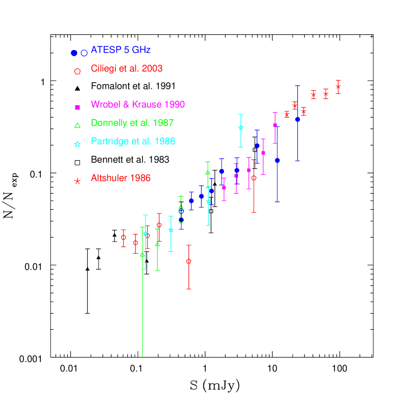
Figure 10: Normalized 5 GHz differential source counts for different samples: Ciliegi et al. 2003 (empty pentagons), Fomalont et al. 1991 (filled triangles), Wrobel & Krause 1990 (filled squares), Donnelly et al. 1987 (empty triangles), Partridge et al. 1986 (stars), Altshuler 1986 (asterisks), Bennett et al. 1983 (empty squares). The ATESP 5 GHz source counts presented here (filled circles plus single empty circle) are corrected for resolution bias as explained in the text. Vertical bars represent Poissonian errors on the normalized counts.

Table 3: ATESP 5 GHz source counts.

$\Delta S$	$<S>$	$N_{S}$	$dN/dS$	$N/N_{\rm exp}$
(mJy)	(mJy)		sr-1 Jy-1
0.37 – 0.52	0.44	22	$6.92\times 10^{8}$	0.031${}_{-0.007}^{+0.008}$
0.52 – 0.74	0.62	24	$4.67\times 10^{8}$	0.050${}_{-0.010}^{+0.010}$
0.74 – 1.05	0.88	17	$2.20\times 10^{8}$	0.056${}_{-0.014}^{+0.017}$
1.05 – 1.48	1.24	12	$1.05\times 10^{8}$	0.064${}_{-0.018}^{+0.024}$
1.48 – 2.09	1.76	12	$7.24\times 10^{7}$	0.104${}_{-0.030}^{+0.040}$
2.09 – 4.19	2.96	12	$2.06\times 10^{7}$	0.106${}_{-0.031}^{+0.040}$
4.19 – 8.37	5.92	8	$6.74\times 10^{6}$	0.197${}_{-0.070}^{+0.094}$
8.37 – 16.7	11.8	2	$8.26\times 10^{5}$	0.137${}_{-0.088}^{+0.180}$
16.7 – 33.5	23.7	2	$4.06\times 10^{5}$	$0.380_{-0.245}^{+0.502}$

We used the 111 5 GHz ATESP sources to derive the differential source counts as a function of flux density. In computing the counts we have used the catalogue as defined at low resolution to minimize incompleteness induced by resolution effects. Integrated flux densities were used for extended sources and peak flux densities for point-like sources.

Each source has been weighted for the reciprocal of its visibility area ($\Omega(S_{\rm peak})/\Omega_{\rm tot}$, see Fig. 5), that is the fraction of the total area over which the source could be detected. We notice that for $S_{\rm peak}>0.5$ mJy a source can be counted over the whole survey area. Moreover, we have taken properly into account the catalogue incompleteness in terms of integrated flux density, due to the resolution bias discussed in the previous section. The correction $c$ for the resolution bias has been defined following Prandoni et al. (2001a) as:

$$c=\frac{1}{1-h(>\Theta_{\rm lim})}$$ (3)

where $h(>\Theta_{\rm lim})$ is the integral angular size distribution proposed by Windhorst et al. (1990) for 1.4 GHz samples, which turned out to be a good representation of the ATESP 5 GHz source sizes at least down to $S\sim 0.7$ mJy (see Sect. 6.2). Here we transform the Windhorst et al. relation to 5 GHz using $\alpha=-0.5$, chosen as reference value (see also Sect. 7.2).

$\Theta_{\rm lim}$ represents the angular size upper limit, above which we expect to be incomplete. This is defined as a function of the integrated source flux density as (see Prandoni et al. 2001a):

$$\Theta_{\rm lim}=\mbox{max}[\Theta_{\rm min},\Theta_{\rm max}]$$ (4)

where $\Theta_{\rm min}$ and $\Theta_{\rm max}$ are the parameters defined in Sect. 6.2. The $\Theta_{\rm min}-S$ relation (red upper solid line in Fig. 9) is important at low flux levels where $\Theta_{\rm max}$ (black dot-dashed line in Fig. 9) becomes unphysical (i.e. $\rightarrow 0$). In other words, introducing $\Theta_{\rm min}$ in the equation takes into account the effect of having a finite synthesized beam size (that is $\Theta_{\rm lim}>>0$ at the survey limit) and a deconvolution efficiency which varies with the source peak flux.

The 5 GHz ATESP source counts are shown in Fig. 10 (filled circles) and listed in Table 3, where, for each flux interval ($\Delta S$), the geometric mean of the flux density ($<S>$), the number of sources detected ($N_{S}$), the differential source density ($dN/dS$) and the normalized differential counts ($N/N_{\rm exp}$) are given. Also listed are the Poissonian errors (calculated following Regener 1951) associated to the normalized counts. For comparison with other 5 GHz studies, the source counts are normalized to a non evolving Euclidean model which fits the brightest sources in the sky. We notice that at 5 GHz the standard Euclidean integral counts are $N(>S)=60\times S^{-1.5}$ sr^-1 ($S$ in Jy).

In determining the resolution bias incompleteness, correct definitions of $h(>\Theta_{\rm lim})$ and $\Theta_{\rm lim}$ could be very important. We checked the robustness of the resolution bias correction by setting different values for $\alpha$ when transforming $h(>\Theta_{\rm lim})$ to 5 GHz and we changed the definition of $\Theta_{\rm lim}$. In particular we tested the effect of setting a fixed value for $\Theta_{\rm min}$ in Eq. (4). In this case $\Theta_{\rm min}$ was set equal to $4\arcsec$, which roughly represents the typical minimum angular size that is reliably deconvolved at low resolution (see Fig. 9). This latter definition has the effect of increasing the resolution bias correction at the faintest fluxes. The same happens when decreasing the spectral index from 0 to -0.7. In general, however, significant changes in the normalized counts are seen only for the faintest flux bin. To illustrate such effect at low fluxes, in Fig. 10 we add the point obtained by computing the resolution bias correction $c$ with $\Theta_{\rm min}=4\arcsec$ and $\alpha=-0.7$ (empty circle at $S=0.44$ mJy).

The ATESP source counts are compared with previous determinations at 5 GHz. As illustrated in Fig. 10 the ATESP counts are consistent with others reported in the literature and improve significantly the statistics available in the flux range $0.4-1$ mJy. The ATESP 5 GHz counts do not show evidence of flattening or slope change down to the survey limit. This fact is discussed in view of the spectral index properties of the ATESP radio sources in Sect. 7.2.

7.2 $1.4-5$ GHz spectral index analysis

Table 4: $1.4-5$ GHz spectral index of ATESP sources.

5 GHz IAU name	1.4 GHz IAU name	$S_{\rm 5\,GHz}$	$S_{\rm 1.4\,GHz}$	$\alpha\;\pm\;\sigma(\alpha)$	5 GHz IAU name	1.4 GHz IAU name	$S_{\rm 5\,GHz}$	$S_{\rm 1.4\,GHz}$	$\alpha\;\pm\;\sigma(\alpha)$
(ATESP5 J…)	(ATESP J…)	(mJy)	(mJy)		(ATESP5 J…)	(ATESP J…)	(mJy)	(mJy)
J224502-400415	J224502-400415	0.65	1.12	$-0.43\pm 0.21$	-	J224911-400859	0.36	0.88	$-0.70\pm 0.33$
J224509-400622	J224509-400623	0.70	2.45	$-0.98\pm 0.16$	-	J224917-401330	$<$0.19	0.61	$<-0.92$
J224510-401655	J224510-401657	0.46	0.57	$-0.17\pm 0.36$	J224919-400037	J224919-400037	0.64	0.91	$-0.28\pm 0.23$
J224513-400052	J224513-400051	0.46	0.59	$-0.20\pm 0.34$	J224932-395801	J224932-395800	0.45	0.55	$-0.16\pm 0.36$
-	J224513-400407	0.27	0.58	$-0.60\pm 0.48$	J224935-400816	J224935-400816	0.82	0.70	$0.12\pm 0.23$
J224516-401807	J224516-401807	3.87	9.54	$-0.71\pm 0.04$	J224948-395918	J224948-395920	1.72	0.87	$0.54\pm 0.17$
J224518-401001	J224518-401001	5.60	10.37	$-0.48\pm 0.02$	J224951-402035	J224951-402233	0.50	1.62	$-0.92\pm 0.24$
J224530-401141	-	0.88	0.49	$0.46\pm 0.30$	J224958-395855	J224958-395855	1.65	1.52	$0.06\pm 0.12$
J224533-402014	J224533-402015	0.53	1.04	$-0.53\pm 0.27$	J225004-402412	J225004-402413	1.78	3.16	$-0.45\pm 0.08$
J224534-401337	J224534-401337	1.86	3.79	$-0.56\pm 0.07$	J225008-400425	J225008-400425	1.70	2.88	$-0.41\pm 0.09$
J224534-400049	J224534-400050	1.87	6.02	$-0.92\pm 0.07$	-	J225009-400605	0.40	0.84	$-0.58\pm 0.34$
-	J224535-402531	$<$0.20	0.57	$<-0.82$	J225028-400333	J225029-400332	0.42	0.75	$-0.46\pm 0.34$
J224547-400324	J224547-400324	28.28	32.83	$-0.12\pm 0.01$	J225034-401936	J225034-401936	25.78	76.62	$-0.856\pm 0.004$
J224550-402021	J224550-402022	1.75	3.54	$-0.55\pm 0.08$	J225048-400147	-	0.96	0.60	$0.37\pm 0.27$
J224551-401618	J224551-401619	0.57	1.16	$-0.56\pm 0.24$	J225056-402254	-	0.43	0.41	$0.04\pm 0.45$
J224557-400934	J224557-400931	0.42	1.35	$-0.92\pm 0.28$	J225056-400033	J225056-400033	2.27	1.17	$0.52\pm 0.14$
J224559-402122	J224558-402122	1.72	5.59	$-0.93\pm 0.08$	J225057-401522	J225057-401522	3.00	2.01	$0.31\pm 0.08$
J224601-401502	J224601-401502	2.58	6.67	$-0.75\pm 0.05$	J225058-401645	-	0.50	0.45	$0.08\pm 0.41$
J224608-400414	J224608-400415	0.61	0.59	$0.03\pm 0.29$	J225100-400934	J225100-400933	0.49	1.65	$-0.95\pm 0.24$
J224613-401132	J224613-401132	1.24	2.23	$-0.46\pm 0.11$	J225112-402230	J225112-402229	1.03	3.06	$-0.86\pm 0.13$
J224623-400854	J224623-400856	0.68	2.26	$-0.94\pm 0.17$	J225118-402653	J225118-402652	2.85	3.69	$-0.20\pm 0.06$
-	J224623-401845	0.41	1.44	$-0.99\pm 0.31$	J225122-402524	J225122-402524	0.54	1.56	$-0.83\pm 0.24$
J224628-401207	J224628-401207	0.82	1.35	$-0.39\pm 0.17$	J225138-401747	J225138-401747	0.62	1.61	$-0.75\pm 0.20$
J224632-400319	J224632-400320	0.72	1.83	$-0.73\pm 0.18$	J225154-401051	J225155-401050	1.31	1.52	$-0.12\pm 0.12$
-	J224640-401710	0.27	0.65	$-0.69\pm 0.47$	-	J225206-401947	0.33	1.25	$-1.05\pm 0.36$
J224646-400829	J224646-400830	13.25	38.2	$-0.83\pm 0.01$	J225207-400720	J225207-400720	4.06	8.99	$-0.62\pm 0.03$
J224647-401220	J224647-401220	0.81	1.17	$-0.29\pm 0.18$	J225217-402135	J225217-402136	1.73	2.16	$-0.17\pm 0.09$
-	J224648-400250	$<$0.20	1.68	$<-1.67$	J225223-401841	J225223-401843	0.85	0.98	$-0.11\pm 0.20$
J224654-400107	J224654-400108	3.15	5.59	$-0.45\pm 0.05$	J225224-402549	J225224-402549	4.76	7.19	$-0.32\pm 0.03$
-	J224658-401206	$<$0.22	0.54	$<-0.71$	J225239-401949	J225239-401948	1.18	2.26	$-0.51\pm 0.12$
J224701-402646	J224701-402645	1.33	2.76	$-0.57\pm 0.11$	J225242-395949	J2252342-395949	0.53	1.48	$-0.81\pm 0.22$
J224702-400948	J224702-400946	0.60	0.61	$-0.01\pm 0.29$	J225249-401256	J225249-401256	1.09	1.52	$-0.26\pm 0.14$
J224707-400616	J224707-400616	1.70	3.37	$-0.54\pm 0.08$	J225316-401200	J225316-401200	0.50	0.78	$-0.35\pm 0.28$
J224714-401453	J224714-401454	3.52	6.26	$-0.45\pm 0.04$	J225321-402317	J225321-402319	1.21	2.32	$-0.51\pm 0.11$
J224714-402400	-	0.57	0.45	$0.19\pm 0.36$	J225322-401931	J225322-401931	1.01	1.86	$-0.48\pm 0.14$
J224719-400141	J224719-400142	0.48	1.32	$-0.79\pm 0.27$	J225323-400453	-	0.85	0.51	$0.40\pm 0.31$
J224719-401530	J224719-401531	0.74	0.84	$-0.10\pm 0.23$	J225325-400221	-	0.53	0.56	$-0.04\pm 0.32$
J224721-402043	-	0.50	0.37	$0.24\pm 0.43$	J225326-395912	J225326-395911	1.77	3.72	$-0.58\pm 0.07$
J224724-395909	J224724-395909	1.45	1.18	$0.16\pm 0.14$	J225332-402721	-	1.00	$<$0.26	$>1.06$
J224727-402751	J224727-402750	0.67	1.94	$-0.84\pm 0.21$	J225334-401414	-	0.54	0.45	$0.14\pm 0.38$
J224727-401926	-	1.11	0.32	$0.98\pm 0.42$	J225344-401928	-	3.52	0.60	$1.39\pm 0.25$
J224729-402000	J224729-402001	0.5	0.84	$-0.41\pm 0.29$	J225345-401845	-	0.48	0.60	$-0.18\pm 0.33$
J224731-400527	-	0.43	0.35	$0.16\pm 0.46$	-	J225351-400441	$<$0.17	0.96	$<-1.36$
J224732-401442	J224732-401442	7.14	20.28	$-0.82\pm 0.02$	J225353-400154	J225353-400153	1.03	1.10	$-0.05\pm 0.17$
J224735-402321	J224735-402321	1.18	1.12	$0.04\pm 0.16$	-	J225354-400241	0.36	1.53	$-1.14\pm 0.31$
J224740-401821	J224740-401821	0.74	2.15	$-0.84\pm 0.18$	J225400-402204	J225400-402204	0.54	1.25	$-0.66\pm 0.24$
J224741-400442	J224741-400443	0.52	0.61	$-0.13\pm 0.31$	J225404-402226	J225404-402226	3.80	10.34	$-0.79\pm 0.03$
J224748-401324	J224748-401324	3.97	14.52	$-1.02\pm 0.03$	J225414-400853	J225414-400852	1.95	3.10	$-0.36\pm 0.07$
J224750-400148	J224750-400143	6.09	13.44	$-0.62\pm 0.02$	J225426-402442	J225426-402442	4.24	10.43	$-0.71\pm 0.03$
J224753-400455	J224753-400456	0.67	2.08	$-0.89\pm 0.19$	J225430-400334	-	0.63	$<$0.26	$>0.70$
-	J224759-400825	0.21	0.82	$-1.07\pm 0.56$	-	J225430-402329	0.36	1.10	$-0.88\pm 0.32$
J224801-400542	-	0.45	0.49	$-0.07\pm 0.38$	J225434-401343	J225434-401343	7.80	21.09	$-0.78\pm 0.01$
-	J224801-395900	0.40	0.69	$-0.43\pm 0.36$	J225435-395931	-	0.71	0.41	$0.43\pm 0.39$
-	J224803-400513	$<$0.20	0.67	$<-0.95$	J225436-400531	-	0.60	0.47	$0.19\pm 0.36$
J224806-402102	J224806-402101	0.80	2.52	$-0.90\pm 0.16$	J225442-400353	-	0.56	$<$0.26	$>0.60$
J224809-402211	J224809-402212	1.26	4.23	$-0.95\pm 0.10$	J225443-401147	-	0.41	$<$0.26	$>0.36$
-	J224811-402455	0.28	0.59	$-0.59\pm 0.48$	J225449-400918	J225449-400918	0.86	1.24	$-0.29\pm 0.17$
-	J224817-400819	0.31	0.54	$-0.44\pm 0.43$	J225450-401639	-	0.61	$<$0.26	$>0.67$
J224822-401808	J224822-401808	10.34	19.08	$-0.48\pm 0.01$	J225504-400154	J225504-400154	4.59	9.67	$-0.59\pm 0.03$
J224827-402515	J224827-402515	0.80	0.58	$0.25\pm 0.27$	J225505-401301	-	0.37	0.51	$-0.25\pm 0.40$
-	J224828-395814	$<$0.20	0.67	$<-0.95$	J225509-402658	J225509-402658	5.18	8.15	$-0.36\pm 0.03$
-	J224843-400456	$<$0.18	0.72	$<-1.09$	J225511-401513	J225512-401513	0.58	0.71	$-0.16\pm 0.27$
J224850-400027	J224850-400027	1.37	1.10	$0.17\pm 0.14$	J225515-401835	J225515-401835	0.42	1.07	$-0.73\pm 0.29$
J224858-402708	J224858-402707	0.50	0.96	$-0.51\pm 0.26$	J225526-400112	J225526-400111	0.41	1.55	$-1.04\pm 0.28$
J224903-400946	J224903-400949	0.96	2.81	$-0.84\pm 0.12$	J225529-401101	J225529-401101	1.09	1.48	$-0.24\pm 0.14$
J224906-402337	J224906-402337	2.48	3.01	$-0.15\pm 0.06$

Figure 11: Top: 1.4 – 5 GHz spectral index vs. 1.4 GHz flux density for the ATESP sample. Only sources catalogued at 1.4 GHz ($S_{\rm peak}({\rm 1.4\,GHz})\geq 6\sigma$) are shown. Open circles with arrows indicate spectral index upper limits due to sources undetected at 5 GHz (the solid line indicates the $3\sigma$ detection limit). Horizontal dotted lines show the $\alpha=0$ and the $\alpha=-0.5$ loci. Circled dots refer to sources displaying a multiple-component/extended radio morphology (either at 1.4 or 5 GHz, either at low or full resolution), typical of AGN–driven radio galaxies. Bottom: Spectral index distribution for the same sources shown above. Shaded histogram refer to upper limits. The vertical dashed line indicates the median spectral index value of the sample ($\alpha_{\rm med}=-0.57$).

Figure 12: Top: 1.4 – 5 GHz spectral index vs. 5 GHz flux density for the ATESP sample. Only sources catalogued at 5 GHz ($S_{\rm peak}({\rm 5\,GHz})\geq 6\sigma$) are shown. Open circles with arrows indicate spectral index lower limits due to sources undetected at 1.4 GHz (the solid line indicates the $3\sigma$ detection limit). Horizontal dotted lines indicate the $\alpha=0$ and the $\alpha=-0.5$ loci. Circled dots refer to sources displaying a multiple-component/extended radio morphology (either at 1.4 or 5 GHz, either at low or full resolution), typical of AGN–driven radio galaxies. Bottom: Spectral index distribution for the same sources shown above. Shaded histogram refer to lower limits. The vertical dashed line indicates the median spectral index value of the sample ($\alpha_{\rm med}=-0.40$).

For the analysis of the $1.4-5$ GHz spectral index properties of the ATESP radio sources, we extracted from the ATESP 1.4 GHz catalogue (Prandoni et al., 2000b), the list of sources located in the $2\times 0.5$ sq. degr. region surveyed at 5 GHz. Of the 109 1.4 GHz sources found, 89 are catalogued also at 5 GHz, whereas the remaining 20 sources are catalogued only at 1.4 GHz. Similarly we have 22 sources which are catalogued only at 5 GHz, for a total of 131 (1.4 and/or 5 GHz) ATESP sources in the overlapping region. In order to exploit the whole sample of 131 sources for the spectral index analysis, we searched for counterparts of the 42 ($20+22$) sources catalogued only at 1.4 (or 5 GHz) down to a $3\sigma$-threshold ($\sim 0.2$ mJy), by directly inspecting the low resolution 5 GHz (or the 1.4 GHz) ATESP radio mosaics, at the source position. This allows us to probe deeper fluxes than with the 89 ATESP sources catalogued at both 1.4 and 5 GHz ($S_{\rm peak}>6\sigma\sim 0.4-0.5$ mJy).

The result of this search is reported in Table 4, where, for each source, we list the 5 GHz and/or 1.4 GHz ATESP IAU source name (Columns 1 and 2), the 5 GHz (low resolution) and 1.4 GHz flux density used for the spectral index derivation (Columns 3 and 4), the $1.4-5$ GHz spectral index with its standard deviation (Column 5).

We notice that flux densities reported in Table 4 are integrated values for resolved sources and peak values for either point-like sources or $<6\sigma$ detections. For undetected sources $3\sigma_{\rm local}$ upper limits are provided. In addition, 1.4 GHz flux densities are corrected for systematic effects (e.g. clean bias and radial smearing), following the recipe derived in Prandoni et al. 2000b (Appendix B).

In summary we have that 118 of the 131 ATESP sources are detected at both frequencies (down to a $3\sigma$-threshold), 5 are detected only at 5 GHz and 8 only at 1.4 GHz.

Figures 11 and 12 show the $1.4$–$5$ GHz spectral index as a function of flux density, for the 109 sources catalogued at 1.4 GHz and for the 111 sources catalogued at 5 GHz respectively (see top panels). Also plotted are the spectral index distributions at the two frequencies (bottom panels). As expected for higher frequency selected samples, the median spectral index is flatter at 5 GHz ($\alpha_{\rm med}=-0.40$) than at 1.4 GHz ($\alpha_{\rm med}=-0.57$) and both samples show a flattening (much more evident at 5 GHz) going to lower flux densities (see Table 5). For $S_{\mbox{1.4 GHz}}>4$ mJy, $\alpha$ shows a narrow dispersion around a median value of $-0.71$ ($-0.62$ at 5 GHz), as expected for standard synchrotron radio emission. At fainter fluxes, however, almost half ($46\%$) of the sources selected at 1.4 GHz and almost 2/3 ($\sim 63\%$) of the sources selected at 5 GHz show flat spectra ($\alpha>-0.5$), with a significant fraction ($29\%$at 5 GHz) of inverted spectra ($\alpha>0$).

It is worth noticing that, since the 5 GHz survey has been conducted several years later than the 1.4 GHz survey, flux variability could affect the spectral index derivation for a number of sources. In particular, it could explain the most extreme cases (like ultra-steep and/or ultra-inverted sources). On the other hand, the two ultra–steep sources ($\alpha<-1.3$) present in the sample (see Fig. 11), if real, could potentially be associated to very high redshift galaxies.

The flattening of the radio spectral index going from mJy to sub–mJy flux densities found for the ATESP–DEEP1 sample confirms on a much larger statistical basis (131 sources) previous results obtained for smaller ($50-60$ sources) samples (e.g. Donnelly et al 1987; Gruppioni et al. 1997) and agrees with the finding of many flat/inverted radio spectra in $\mu$Jy samples (Fomalont et al. 1991; Windhorst et al 1993). On the other hand, it disagrees with a more recent spectral index analysis performed in the Lockman Hole, where the sources are claimed to have steep–spectrum down to 0.2 mJy (Ciliegi et al. 2003). It is worth noticing, however, that the statistics available to the Ciliegi et al. sample at $S_{\rm 5\,GHz}>0.2$ mJy is very poor.

It is interesting to compare the spectral index statistics reported in Table 5 (upper limits are included by using the survival analysis methods presented in Feigelson & Nelson (1985) and Isobe et al. (1986)) to the one obtained in samples selected at the same frequencies (1.4 and 5 GHz). As mentioned above, a general agreement is found: Fomalont et al. (1991) report a $\alpha_{med}=-0.38$ and a $f(\alpha>-0.5)=60\%$ at fluxes $16<S_{\rm 5\leavevmode\nobreak\ GHz}<1000$ $\mu$Jy; while Donnelly et al. (1987) report $\alpha_{mean}=-0.31\pm 0.58$, $\alpha_{med}=-0.42$ and $f(\alpha>-0.5)=50\%$ at $0.4<S_{\rm 5\leavevmode\nobreak\ GHz}<1.2$ mJy. On the other hand, a somewhat steeper behaviour was found also by Donnelly et al. (1987) at 1.4 GHz: $\alpha_{mean}=-0.80\pm 0.49$, $\alpha_{med}=-0.76$ and $f(\alpha>-0.5)=22\%$ at $0.5<S_{\rm 1.4\leavevmode\nobreak\ GHz}<3$ mJy, which was interpreted as due to a significantly different composition of the faint radio population depending on the selection frequency.

Indeed the ATESP 1.4 and 5 GHz selected samples have in common only 2/3 of the sources (89/131). This can explain not only the somewhat different spectral properties of the two samples at low flux densities ($S<4$ mJy), but also why a significant flattening of source counts in 1.4 GHz-selected samples at $S\la 1$ mJy does not necessarily result in a flattening of the 5 GHz source counts in the flux range covered by the ATESP sample. By assuming as reference $\alpha=-0.53$ (the median spectral index found for the sub-mJy 1.4 GHz selected ATESP sources, see Tab. 5), we expect the flattening to occur at $S_{\rm 5\,GHz}\sim 0.5$ mJy, that is very close to the flux density limit of the 5 GHz ATESP survey.

As a final remark we notice that radio sources with a multiple–component/extended radio morphology, typical of classical AGN–driven radio galaxies, are both shown as circled dots in Figs. 11 and 12. It is evident that such sources are characterized by steep synchrotron radio spectra and are mainly found at mJy flux densities. On the other hand unresolved multiple–component sources can be present also at lower fluxes, where most of the sources could not be successfully deconvolved, due to the poorer deconvolution efficiency (see § 6.2). Higher spatial resolution radio data are needed to assess whether radio emission in sub-mJy flat sources is triggered by active nuclei or large-scale star formation.

Table 5: Spectral index statistics

Flux range	N	$\alpha_{\rm mean}$	$\alpha_{\rm med}$	$N_{\alpha>-0.5}$	$N_{\alpha>0}$
1.4 GHz
Any flux	109	$-0.56\pm 0.04$	$-0.57$	47 (43%)	10 (9%)
$S>4$ mJy	22	$-0.66\pm 0.05$	$-0.71$	7 (32%)	-
$S\leq 4$ mJy	87	$-0.53\pm 0.05$	$-0.53$	40 (46%)	10 (11%)
5 GHz
Any flux	111	$-0.28\pm 0.05$	$-0.40$	67 (60%)	28 (25%)
$S>4$ mJy	13	$-0.58\pm 0.06$	$-0.62$	5 (38%)	-
$S\leq 4$ mJy	98	$-0.24\pm 0.06$	$-0.29$	62 (63%)	28 (29%)

8 Summary

We used the ATCA to follow-up at 5 GHz part of the region previously covered by the sub–mJy ATESP 1.4 GHz survey (Prandoni et al. 2000a,b). In particular, we imaged a 1 sq. degr. area where, in addition to the 1.4 GHz information, extensive $UBVRI$ deep optical imaging is available (Mignano et al. 2006). The 5 GHz survey was designed to have uniform sensitivity over the entire region observed.

In order to be able to measure the 1.4 - 5 GHz spectral index, we produced 5 GHz images at exactly the same resolution (same size in pixels and restoring beam) as the 1.4 GHz mosaics (see Prandoni et al. 2000a ). On the other hand, full resolution ($\sim 2\arcsec$) mosaics were also produced. As expected, the noise level obtained, $\sim 70$ $\mu$Jy, is fairly uniform within each mosaic and from mosaic to mosaic.

We used the low resolution images for the source extraction: we produced a catalogue of 111 radio sources, complete down to $S\sim 0.4$ mJy ($6\sigma$). The full resolution information was used to assess size and radio morphology of the catalogued sources. A detailed analysis of the source sizes shows that the ATESP 5 GHz sources can be satisfactorily described by the angular size distribution proposed by Windhorst et al. (1990), at least down to $S>0.7-1$ mJy. Below such limit, the high number of sources which remain unresolved even at full resolution prevents us from a reliable analysis. We can only argue that our upper limits ($<1-2\arcsec$) are consistent with the result of Fomalont et al. (1991), who find $\Theta<1.5\arcsec$ for sources with $0.06<S(\rm{5GHz})<0.8$ mJy. Also consistent is the result of Bondi et al. (2003) who find $\Theta_{med}=1.\arcsec 8\pm 0.\arcsec 2$. We notice that Bondi et al. suggest a steeper distribution than the one of Windhorst et al. for sources $0.4<S(\rm{1.4GHz})<1$ mJy.

We have derived the $\log{N}-\log{S}$ relation for the ATESP 5 GHz catalogue. The possible causes of incompleteness at the faint end of the source counts have been taken into account, with particular respect to resolution effects (resolution bias). The ATESP 5 GHz counts are consistent with the counts derived from other 5 GHz surveys and improve significantly the statistics of the counts in the flux range $0.4-1$ mJy. The ATESP 5 GHz counts do not show evidence of flattening down to the survey limit.

The $1.4-5$ GHz spectral index was derived for all the ATESP radio sources present in the $2\times 0.5$ sq. degr. region surveyed at both 1.4 and 5 GHz. A flattening of the spectral index with decreasing flux densities was found, which is particularly significant for the 5 GHz selected sample. At mJy level we have mostly steep-spectrum ($\alpha\sim-0.7$) synchrotron radio sources, while at sub-mJy flux densities we have a composite population, with $\sim 60\%$ of the 5 GHz sources showing flat spectra and a significant fraction ($\sim 30\%$ at 5 GHz) of inverted-spectrum sources. The spectral index flattening of the 1.4 GHz selected sample is somewhat milder, with $\alpha_{\rm med}=-0.53$ at sub-mJy flux densities against a value of $\alpha_{\rm med}=-0.29$ found for the 5 GHz sources.

We notice that, when we take into account the spectral index properties of the ATESP 1.4 GHz selected sample, as inferred by our 1.4/5 GHz measurements, we can expect the 5 GHz source counts to flatten at flux densities $\sim 0.5$ mJy, that is very close to the flux density limit of the 5 GHz ATESP survey. This explains why we do not yet see evidence of such a flattening in the ATESP 5 GHz source counts.

Particularly interesting is the possibility of combining the spectral index information with other observational properties to infer the nature of the faint radio population, with particular respect to flat/inverted–spectrum sources, and assess the physical processes triggering the radio emission in those sources. This kind of analysis needs information about redshifts and types of the galaxies hosting the radio sources. A detailed radio/optical study of our sample is possible, thanks to the extensive optical coverage available to it (see Sect. 2), and is the subject of the second paper of this series (Mignano et al., in prep.).

Table 6: The 5 GHz Catalogue

	low resolution parameters									full resolution parameters
IAU Name	R.A.	DEC.	$S_{\rm peak}$	$S_{\rm total}$	$\Theta_{\rm maj}$	$\Theta_{\rm min}$	P.A.		$\sigma_{\rm local}$	R.A.	DEC.	$S_{\rm peak}$	$S_{\rm total}$	$\Theta_{\rm maj}$	$\Theta_{\rm min}$	P.A.		$\sigma_{\rm local}$
	(J2000)		mJy		arcsec		degr.		$\mu$Jy	(J2000)		mJy		arcsec		degr.		$\mu$Jy
ATESP5 J224502-400415	22 45 02.86	-40 04 15.4	0.65	0.62	0.00	0.00	0.0	S	67	22 45 02.83	-40 04 14.7	0.43	0.60	1.86	1.14	-42.9	S*	69
ATESP5 J224509-400622	22 45 09.40	-40 06 22.8	0.70	0.67	0.00	0.00	0.0	S	61	22 45 09.38	-40 06 23.0	0.53	0.72	2.50	0.35	-27.9	S	67
ATESP5 J224510-401655	22 45 10.00	-40 16 55.2	0.46	0.66	0.00	0.00	0.0	S*	75	22 45 09.99	-40 16 56.8	0.34					D	74
ATESP5 J224513-400052	22 45 13.46	-40 00 52.3	0.46	0.44	0.00	0.00	0.0	S	72	22 45 13.51	-40 00 51.1	0.33					D	76
ATESP5 J224516-401807	22 45 16.70	-40 18 07.8	1.62	3.87	18.38	0.00	0.0	M
ATESP5 J224516-401807A	22 45 15.86	-40 17 58.5	0.69	1.04	9.03	0.00	-81.2	S	76	22 45 16.01	-40 17 58.5	0.37					D	72
ATESP5 J224516-401807B	22 45 17.01	-40 18 11.3	1.62	2.83	12.58	4.81	-26.4	S	76	22 45 16.70	-40 18 05.9	0.54	0.59	0.00	0.00	0.0	S(a)	72
										22 45 17.13	-40 18 13.7	0.54	2.08	11.40	5.27	-11.7	E	72
ATESP5 J224518-401001	22 45 18.70	-40 10 01.6	5.60	5.65	0.00	0.00	0.0	S	59	22 45 18.69	-40 10 01.7	4.54	5.03	1.68	0.00	32.5	S	85
ATESP5 J224530-401141	22 45 30.30	-40 11 41.8	0.88	0.75	0.00	0.00	0.0	S	69	22 45 30.30	-40 11 41.3	0.67	0.73	0.00	0.00	0.0	S	67
ATESP5 J224533-402014	22 45 33.03	-40 20 14.6	0.53	0.53	0.00	0.00	0.0	S	74	22 45 33.10	-40 20 15.7	0.39					D	66
ATESP5 J224534-401337	22 45 34.37	-40 13 37.2	1.17	1.86	10.52	4.12	32.4	S	71	22 45 34.49	-40 13 34.1	0.38	1.12	8.32	5.19	40.8	DE(b)	69
ATESP5 J224534-400049	22 45 34.33	-40 00 49.4	1.54	1.87	7.66	1.31	-2.4	S	73	22 45 34.31	-40 00 47.6	0.98	1.26	1.83	1.10	-9.9	S	94
ATESP5 J224547-400324	22 45 47.88	-40 03 24.2	26.86	28.28	3.79	0.00	46.1	S	78	22 45 47.86	-40 03 24.2	18.89	21.44	1.55	0.00	34.8	S	184
ATESP5 J224550-402021	22 45 50.47	-40 20 21.8	0.60	1.75	28.89	20.23	-71.2	E	74	22 45 50.55	-40 20 26.3	0.25					D(c)	73
ATESP5 J224551-401618	22 45 51.30	-40 16 18.8	0.57	0.54	0.00	0.00	0.0	S	73	22 45 51.29	-40 16 20.1	0.40					D	76
ATESP5 J224557-400934	22 45 57.79	-40 09 34.1	0.42	0.52	0.00	0.00	0.0	S	66	22 45 57.83	-40 09 34.2	0.29					D	80
ATESP5 J224559-402122	22 45 59.03	-40 21 22.0	1.09	1.72	20.00	0.00	0.0	M
ATESP5 J224559-402122A	22 45 57.99	-40 21 22.8	0.70	0.70	0.00	0.00	0.0	S	73	22 45 57.97	-40 21 23.7	0.61	0.69	0.00	0.00	0.0	S	73
ATESP5 J224559-402122B	22 45 59.74	-40 21 21.5	1.09	1.02	0.00	0.00	0.0	S	73	22 45 59.73	-40 21 21.9	0.81	0.95	2.19	0.00	-11.6	S	73
ATESP5 J224601-401502	22 46 01.50	-40 15 02.9	2.58	2.55	0.00	0.00	0.0	S	69	22 46 01.49	-40 15 02.4	2.11	2.44	1.26	0.58	64.1	S	73
ATESP5 J224608-400414	22 46 08.44	-40 04 14.5	0.61	0.74	0.00	0.00	0.0	S	68	22 46 08.47	-40 04 15.4	0.48					D	83
ATESP5 J224613-401132	22 46 13.17	-40 11 32.2	1.24	1.28	0.00	0.00	0.0	S	70	22 46 13.15	-40 11 32.4	0.95	0.97	0.00	0.00	0.0	S	63
ATESP5 J224623-400854	22 46 23.35	-40 08 54.7	0.68	0.69	0.00	0.00	0.0	S	67	22 46 23.33	-40 08 56.3	0.60	0.70	0.00	0.00	0.0	S*	80

Table 6: The 5 GHz Catalogue (continued)

	low resolution parameters									full resolution parameters
IAU Name	R.A.	DEC.	$S_{\rm peak}$	$S_{\rm total}$	$\Theta_{\rm maj}$	$\Theta_{\rm min}$	P.A.		$\sigma_{\rm local}$	R.A.	DEC.	$S_{\rm peak}$	$S_{\rm total}$	$\Theta_{\rm maj}$	$\Theta_{\rm min}$	P.A.		$\sigma_{\rm local}$
	(J2000)		mJy		arcsec		degr.		$\mu$Jy	(J2000)		mJy		arcsec		degr.		$\mu$Jy
ATESP5 J224628-401207	22 46 28.46	-40 12 07.4	0.82	0.94	0.00	0.00	0.0	S	68	22 46 28.46	-40 12 07.3	0.57	0.71	0.00	0.00	0.0	S	76
ATESP5 J224632-400319	22 46 32.88	-40 03 19.0	0.72	0.75	0.00	0.00	0.0	S	69	22 46 32.89	-40 03 19.1	0.42	0.88	3.41	1.86	-88.3	S	69
ATESP5 J224646-400829	22 46 46.52	-40 08 29.6	8.93	13.25	11.65	0.00	32.5	S	70	22 46 46.26	-40 08 33.8	2.79	4.62	3.19	1.57	23.4	S(d)	96
										22 46 46.64	-40 08 28.2	3.70	7.26	5.36	1.09	7.4	S	96
ATESP5 J224647-401220	22 46 47.66	-40 12 20.7	0.81	0.66	0.00	0.00	0.0	S	69	22 46 47.65	-40 12 21.5	0.64	0.83	2.84	0.00	16.0	S	73
ATESP5 J224654-400107	22 46 54.53	-40 01 07.2	1.17	3.15	36.66	27.04	89.8	E	73	22 46 54.55	-40 01 06.1	0.49	0.70	2.86	0.67	36.9	S*(e)	73
ATESP5 J224701-402646	22 47 01.48	-40 26 46.1	1.08	1.33	5.72	1.88	48.5	S	79	22 47 01.48	-40 26 45.9	0.74	1.00	2.43	1.03	-15.8	S	74
ATESP5 J224702-400948	22 47 02.08	-40 09 48.1	0.60	0.57	0.00	0.00	0.0	S	70	22 47 02.03	-40 09 48.6	0.41					D	75
ATESP5 J224707-400616	22 47 07.50	-40 06 16.6	1.70	1.76	0.00	0.00	0.0	S	71	22 47 07.51	-40 06 16.6	1.33	1.51	1.88	0.00	40.3	S	73
ATESP5 J224714-401453	22 47 14.21	-40 14 53.9	2.89	3.52	6.43	0.00	53.2	S	71	22 47 14.19	-40 14 54.4	1.45	3.27	4.54	1.74	35.4	S	76
ATESP5 J224714-402400	22 47 14.71	-40 24 00.2	0.57	0.47	0.00	0.00	0.0	S	71	22 47 14.70	-40 24 01.1	0.52	0.44	0.00	0.00	0.0	S	78
ATESP5 J224719-400141	22 47 19.56	-40 01 41.0	0.48	0.56	0.00	0.00	0.0	S*	71	22 47 19.53	-40 01 41.9	0.53	0.49	0.00	0.00	0.0	S	69
ATESP5 J224719-401530	22 47 19.61	-40 15 30.3	0.74	0.56	0.00	0.00	0.0	S	73	22 47 19.61	-40 15 30.7	0.59	0.61	0.00	0.00	0.0	S	73
ATESP5 J224721-402043	22 47 21.66	-40 20 43.9	0.50	0.57	0.00	0.00	0.0	S	74	22 47 21.60	-40 20 42.5	0.26					D	76
ATESP5 J224724-395909	22 47 24.75	-39 59 09.2	1.18	1.45	6.49	0.22	38.5	S	71	22 47 24.77	-39 59 08.9	1.00	1.02	0.00	0.00	0.0	S	73
ATESP5 J224727-402751	22 47 27.25	-40 27 51.0	0.67	0.59	0.00	0.00	0.0	S	77	22 47 27.22	-40 27 50.4	0.61	0.52	0.00	0.00	0.0	S	78
ATESP5 J224727-401926	22 47 27.31	-40 19 26.6	1.11	1.12	0.00	0.00	0.0	S	73	22 47 27.30	-40 19 26.3	0.93	1.02	0.00	0.00	0.0	S	72
ATESP5 J224729-402000	22 47 29.42	-40 20 00.5	0.50	0.41	0.00	0.00	0.0	S	73	22 47 29.52	-40 20 01.3	0.35					D	75
ATESP5 J224731-400527	22 47 31.58	-40 05 27.8	0.43	0.34	0.00	0.00	0.0	S	67	22 47 31.63	-40 05 28.7	0.28					D	76
ATESP5 J224732-401442	22 47 32.94	-40 14 42.7	6.07	7.14	7.14	2.51	9.2	S	75	22 47 32.92	-40 14 42.3	3.48	6.05	3.70	1.46	-22.4	S	79
ATESP5 J224735-402321	22 47 35.70	-40 23 21.8	1.18	1.16	0.00	0.00	0.0	S	75	22 47 35.72	-40 23 21.7	1.08	1.27	2.37	0.00	17.4	S	74
ATESP5 J224740-401821	22 47 40.49	-40 18 21.7	0.74	0.62	0.00	0.00	0.0	S	76	22 47 40.53	-40 18 20.5	0.50	0.93	5.65	0.14	8.2	S*	77
ATESP5 J224741-400442	22 47 41.13	-40 04 42.6	0.52	0.48	0.00	0.00	0.0	S	67	22 47 41.15	-40 04 43.4	0.39					D	71
ATESP5 J224748-401324	22 47 48.74	-40 13 24.5	2.97	3.97	6.46	1.95	76.9	S	72	22 47 48.54	-40 13 24.3	1.12	1.81	2.65	1.59	-44.2	S(d)	74
										22 47 48.92	-40 13 25.0	1.07	1.58	2.40	1.53	15.2	S*	74

Table 6: The 5 GHz Catalogue (continued)

	low resolution parameters									full resolution parameters
IAU Name	R.A.	DEC.	$S_{\rm peak}$	$S_{\rm total}$	$\Theta_{\rm maj}$	$\Theta_{\rm min}$	P.A.		$\sigma_{\rm local}$	R.A.	DEC.	$S_{\rm peak}$	$S_{\rm total}$	$\Theta_{\rm maj}$	$\Theta_{\rm min}$	P.A.		$\sigma_{\rm local}$
	(J2000)		mJy		arcsec		degr.		$\mu$Jy	(J2000)		mJy		arcsec		degr.		$\mu$Jy
ATESP5 J224750-400148	22 47 50.03	-40 01 48.6	2.94	6.09	56.13	21.93	53.2	E	72	22 47 50.11	-40 01 48.6	1.15	3.18	5.00	2.77	26.5	S(f)	71
ATESP5 J224753-400455	22 47 53.73	-40 04 55.1	0.67	0.68	0.00	0.00	0.0	S	70	22 47 53.65	-40 04 56.3	0.44	0.78	3.51	0.00	69.4	S*	68
ATESP5 J224801-400542	22 48 01.06	-40 05 42.7	0.45	0.57	0.00	0.00	0.0	S	72	22 48 01.12	-40 05 42.9	0.30					D	70
ATESP5 J224806-402102	22 48 06.64	-40 21 02.3	0.80	0.69	0.00	0.00	0.0	S	72	22 48 06.62	-40 21 01.6	0.72	0.61	0.00	0.00	0.0	S	78
ATESP5 J224809-402211	22 48 09.93	-40 22 11.9	1.26	1.39	0.00	0.00	0.0	S	69	22 48 09.87	-40 22 11.5	0.49	2.01	9.91	5.72	8.7	E	75
ATESP5 J224822-401808	22 48 22.12	-40 18 08.2	10.26	10.34	3.02	0.00	45.5	S	72	22 48 22.12	-40 18 08.3	8.70	9.20	1.05	0.29	8.1	S	86
ATESP5 J224827-402515	22 48 27.20	-40 25 15.7	0.80	0.72	0.00	0.00	0.0	S	66	22 48 27.24	-40 25 15.7	0.70	0.75	0.00	0.00	0.0	S	68
ATESP5 J224850-400027	22 48 50.54	-40 00 27.4	1.37	1.41	0.00	0.00	0.0	S	63	22 48 50.53	-40 00 27.5	1.32	1.36	0.79	0.00	6.0	S	66
ATESP5 J224858-402708	22 48 58.56	-40 27 08.2	0.50	0.52	0.00	0.00	0.0	S	66	22 48 58.52	-40 27 08.4	0.30					D	66
ATESP5 J224903-400946	22 49 03.36	-40 09 46.6	0.67	0.96	11.87	0.00	39.5	S	60	22 49 03.46	-40 09 45.9	0.53	0.57	0.00	0.00	0.0	S	66
ATESP5 J224906-402337	22 49 06.73	-40 23 37.5	2.48	2.36	0.00	0.00	0.0	S	66	22 49 06.69	-40 23 37.7	2.21	2.33	1.01	0.28	10.6	S	72
ATESP5 J224919-400037	22 49 19.35	-40 00 37.2	0.64	0.54	0.00	0.00	0.0	S	66	22 49 19.34	-40 00 37.9	0.73	0.80	0.00	0.00	0.0	S	72
ATESP5 J224932-395801	22 49 32.07	-39 58 01.8	0.45	0.33	0.00	0.00	0.0	S	71	22 49 32.09	-39 58 01.3	0.41					D	75
ATESP5 J224935-400816	22 49 35.21	-40 08 16.9	0.61	0.82	7.55	4.04	17.9	S	63	22 49 35.23	-40 08 16.8	0.57	0.55	0.00	0.00	0.0	S	66
ATESP5 J224948-395918	22 49 48.08	-39 59 18.9	1.72	1.67	0.00	0.00	0.0	S	71	22 49 48.08	-39 59 19.7	1.86	1.94	1.04	0.00	4.5	S	75
ATESP5 J224951-402035	22 49 51.23	-40 20 35.4	0.50	0.60	0.00	0.00	0.0	S	66	22 49 51.18	-40 20 32.6	0.29					D	71
ATESP5 J224958-395855	22 49 58.26	-39 58 55.4	1.65	1.77	0.00	0.00	0.0	S	72	22 49 58.27	-39 58 55.5	1.46	1.62	1.33	0.26	23.8	S	90
ATESP5 J225004-402412	22 50 04.43	-40 24 12.4	1.78	1.76	0.00	0.00	0.0	S	66	22 50 04.42	-40 24 12.5	1.50	1.63	1.27	0.45	0.2	S	76
ATESP5 J225008-400425	22 50 08.82	-40 04 25.5	1.49	1.70	4.86	2.12	-43.6	S	70	22 50 08.81	-40 04 25.3	1.33	1.47	0.94	0.41	64.2	S	69
ATESP5 J225028-400333	22 50 28.92	-40 03 33.3	0.42	0.40	0.00	0.00	0.0	S	68	22 50 28.97	-40 03 32.0	0.35					D	73
ATESP5 J225034-401936	22 50 34.61	-40 19 36.3	15.03	25.78	13.10	0.00	0.0	M
ATESP5 J225034-401933A	22 50 34.28	-40 19 33.8	15.03	16.84	4.11	2.59	-39.1	S	68	22 50 34.26	-40 19 33.5	8.63	13.34	2.48	1.71	16.6	S	116
ATESP5 J225035-401941B	22 50 35.24	-40 19 41.0	8.02	8.94	3.82	2.85	-29.1	S	68	22 50 35.28	-40 19 41.2	4.40	6.55	2.22	1.69	11.5	S	116
ATESP5 J225048-400147	22 50 48.04	-40 01 47.0	0.96	0.75	0.00	0.00	0.0	S	66	22 50 48.05	-40 01 47.0	0.93	1.03	1.14	0.00	-85.6	S	66
ATESP5 J225056-402254	22 50 56.67	-40 22 54.6	0.43	0.40	0.00	0.00	0.0	S	69	22 50 56.65	-40 22 55.0	0.32					D	70
ATESP5 J225056-400033	22 50 56.72	-40 00 33.2	2.12	2.27	3.87	1.72	4.0	S	65	22 50 56.74	-40 00 33.2	1.90	1.96	0.00	0.00	0.0	S	72

Table 6: The 5 GHz Catalogue (continued)

	low resolution parameters									full resolution parameters
IAU Name	R.A.	DEC.	$S_{\rm peak}$	$S_{\rm total}$	$\Theta_{\rm maj}$	$\Theta_{\rm min}$	P.A.		$\sigma_{\rm local}$	R.A.	DEC.	$S_{\rm peak}$	$S_{\rm total}$	$\Theta_{\rm maj}$	$\Theta_{\rm min}$	P.A.		$\sigma_{\rm local}$
	(J2000)		mJy		arcsec		degr.		$\mu$Jy	(J2000)		mJy		arcsec		degr.		$\mu$Jy
ATESP5 J225057-401522	22 50 57.79	-40 15 22.5	2.89	3.00	5.61	0.00	12.8	S	64	22 50 57.79	-40 15 22.5	2.41	2.47	0.00	0.00	0.0	S	76
ATESP5 J225058-401645	22 50 58.30	-40 16 45.6	0.50	0.39	0.00	0.00	0.0	S	70	22 50 58.32	-40 16 44.9	0.29					D	77
ATESP5 J225100-400934	22 51 00.94	-40 09 34.0	0.49	0.46	0.00	0.00	0.0	S	64	22 51 00.96	-40 09 34.0	0.31					D	68
ATESP5 J225112-402230	22 51 12.73	-40 22 30.1	1.03	1.13	0.00	0.00	0.0	S	71	22 51 12.76	-40 22 30.2	0.71	0.85	1.71	0.85	-14.9	S	70
ATESP5 J225118-402653	22 51 18.34	-40 26 53.2	2.64	2.85	3.26	2.25	30.0	S	69	22 51 18.40	-40 26 53.4	1.40	2.84	2.96	2.45	-61.5	S	75
ATESP5 J225122-402524	22 51 22.91	-40 25 24.3	0.54	0.58	0.00	0.00	0.0	S	70	22 51 22.84	-40 25 25.1	0.50	0.46	0.00	0.00	0.0	S	70
ATESP5 J225138-401747	22 51 38.49	-40 17 47.3	0.62	0.64	0.00	0.00	0.0	S	66	22 51 38.58	-40 17 47.5	0.60	0.74	2.83	0.00	5.0	S	71
ATESP5 J225154-401051	22 51 54.97	-40 10 51.1	1.15	1.31	4.95	0.00	-55.3	S	55	22 51 54.96	-40 10 51.4	1.18	1.22	0.00	0.00	0.0	S	66
ATESP5 J225207-400720	22 52 07.48	-40 07 20.6	4.06	4.12	0.00	0.00	0.0	S	57	22 52 07.49	-40 07 20.6	3.53	3.66	0.81	0.10	25.6	S	65
ATESP5 J225217-402135	22 52 17.19	-40 21 35.7	1.73	1.70	0.00	0.00	0.0	S	66	22 52 17.20	-40 21 35.7	1.54	1.63	0.95	0.14	42.5	S	61
ATESP5 J225223-401841	22 52 23.82	-40 18 41.9	0.52	0.85	14.78	0.00	-28.8	S	67	22 52 23.85	-40 18 43.3	0.27					D	72
ATESP5 J225224-402549	22 52 24.79	-40 25 49.1	4.76	4.74	0.00	0.00	0.0	S	55	22 52 24.79	-40 25 49.3	4.47	4.60	0.90	0.00	3.1	S	67
ATESP5 J225239-401949	22 52 39.29	-40 19 49.5	0.68	1.18	10.06	7.33	-5.9	S	68	22 52 39.35	-40 19 47.3	0.31					D(c)	65
ATESP5 J225242-395949	22 52 42.53	-39 59 49.9	0.53	0.42	0.00	0.00	0.0	S	63	22 52 42.58	-39 59 49.6	0.58	0.51	0.00	0.00	0.0	S*	65
ATESP5 J225249-401256	22 52 49.92	-40 12 56.0	1.09	0.93	0.00	0.00	0.0	S	61	22 52 49.90	-40 12 56.3	1.01	1.10	1.81	0.00	-4.7	S	67
ATESP5 J225316-401200	22 53 16.29	-40 12 00.6	0.50	0.52	0.00	0.00	0.0	S	63	22 53 16.27	-40 12 01.1	0.48	0.54	0.00	0.00	0.0	S*	66
ATESP5 J225321-402317	22 53 21.28	-40 23 17.7	0.64	1.21	28.27	11.48	-53.0	E	67	22 53 21.16	-40 23 18.1	0.57	0.59	0.00	0.00	0.0	S*(f)	69
ATESP5 J225322-401931	22 53 22.73	-40 19 31.6	1.01	0.85	0.00	0.00	0.0	S	68	22 53 22.76	-40 19 31.9	1.01	1.04	0.00	0.00	0.0	S	68
ATESP5 J225323-400453	22 53 23.89	-40 04 53.7	0.67	0.85	6.52	2.56	-44.0	S	59	22 53 23.91	-40 04 53.6	0.63	0.64	0.00	0.00	0.0	S	68
ATESP5 J225325-400221	22 53 25.45	-40 02 21.4	0.53	0.28	0.00	0.00	0.0	S	59	22 53 25.43	-40 02 21.5	0.66	0.68	0.00	0.00	0.0	S	69
ATESP5 J225326-395912	22 53 26.96	-39 59 12.6	1.31	1.77	8.60	0.00	54.3	S	63	22 53 27.05	-39 59 11.7	0.75	1.02	1.82	0.96	61.6	S(g)	71
ATESP5 J225332-402721	22 53 32.41	-40 27 21.1	1.00	0.83	0.00	0.00	0.0	S	61	22 53 32.41	-40 27 20.8	1.02	1.02	0.00	0.00	0.0	S	69
ATESP5 J225334-401414	22 53 34.66	-40 14 14.0	0.54	0.52	0.00	0.00	0.0	S	63	22 53 34.65	-40 14 12.4	0.57	0.48	0.00	0.00	0.0	S	65
ATESP5 J225344-401928	22 53 44.89	-40 19 28.6	3.52	3.38	0.00	0.00	0.0	S	64	22 53 44.88	-40 19 28.6	3.36	3.47	0.61	0.00	88.8	S	68
ATESP5 J225345-401845	22 53 45.74	-40 18 45.4	0.48	0.35	0.00	0.00	0.0	S	63	22 53 45.73	-40 18 47.0	0.25					D	70
ATESP5 J225353-400154	22 53 53.32	-40 01 54.1	1.03	0.99	0.00	0.00	0.0	S	62	22 53 53.31	-40 01 54.0	0.99	1.04	0.00	0.00	0.0	S	67
ATESP5 J225400-402204	22 54 00.49	-40 22 04.3	0.54	0.51	0.00	0.00	0.0	S	65	22 54 00.52	-40 22 04.1	0.44	0.62	1.95	0.72	-88.5	S*	68
ATESP5 J225404-402226	22 54 04.33	-40 22 26.9	3.80	3.74	0.00	0.00	0.0	S	63	22 54 04.33	-40 22 26.7	3.38	3.78	1.25	0.57	-17.5	S	71

Table 6: The 5 GHz Catalogue (continued)

	low resolution parameters									full resolution parameters
IAU Name	R.A.	DEC.	$S_{\rm peak}$	$S_{\rm total}$	$\Theta_{\rm maj}$	$\Theta_{\rm min}$	P.A.		$\sigma_{\rm local}$	R.A.	DEC.	$S_{\rm peak}$	$S_{\rm total}$	$\Theta_{\rm maj}$	$\Theta_{\rm min}$	P.A.		$\sigma_{\rm local}$
	(J2000)		mJy		arcsec		degr.		$\mu$Jy	(J2000)		mJy		arcsec		degr.		$\mu$Jy
ATESP5 J225414-400853	22 54 14.57	-40 08 53.0	1.12	1.95	9.05	7.88	-40.8	S	64	22 54 14.54	-40 08 48.8	0.36	0.84	9.76	3.90	-16.2	DE	69
ATESP5 J225426-402442	22 54 26.16	-40 24 42.6	2.06	4.24	34.73	0.00	0.0	M
ATESP5 J225425-402446A	22 54 25.48	-40 24 46.9	2.06	2.19	3.80	0.00	52.6	S	64	22 54 25.43	-40 24 47.2	1.47	2.11	2.02	1.18	42.4	S(h)	70
ATESP5 J225426-402438B	22 54 26.88	-40 24 38.0	1.61	2.05	6.63	0.00	70.8	S	64	22 54 27.01	-40 24 37.0	1.03	2.02	7.92	4.49	60.6	E	70
ATESP5 J225430-400334	22 54 30.47	-40 03 34.0	0.63	0.65	0.00	0.00	0.0	S	60	22 54 30.47	-40 03 34.9	0.58	0.60	0.00	0.00	0.0	S	70
ATESP5 J225434-401343	22 54 34.70	-40 13 43.2	3.17	7.80	22.51	3.07	-33.6	S	58	22 54 34.35	-40 13 37.4	1.59	3.56	3.06	2.27	-60.5	S(dh)	71
										22 54 35.05	-40 13 48.9	1.17	4.38	6.10	2.51	-38.6	S	71
ATESP5 J225435-395931	22 54 35.26	-39 59 31.9	0.71	0.63	0.00	0.00	0.0	S	63	22 54 35.29	-39 59 32.6	0.69	0.71	0.00	0.00	0.0	S	67
ATESP5 J225436-400531	22 54 36.29	-40 05 31.3	0.60	0.65	0.00	0.00	0.0	S	65	22 54 36.24	-40 05 30.8	0.66	0.68	0.00	0.00	0.0	S	66
ATESP5 J225442-400353	22 54 42.64	-40 03 53.0	0.56	0.49	0.00	0.00	0.0	S	60	22 54 42.63	-40 03 53.2	0.54	0.52	0.00	0.00	0.0	S	65
ATESP5 J225443-401147	22 54 43.07	-40 11 47.4	0.41	0.39	0.00	0.00	0.0	S	60	22 54 43.02	-40 11 48.1	0.34					D	71
ATESP5 J225449-400918	22 54 49.73	-40 09 18.6	0.86	0.92	0.00	0.00	0.0	S	64	22 54 49.72	-40 09 18.4	0.72	0.79	0.00	0.00	0.0	S	68
ATESP5 J225450-401639	22 54 50.81	-40 16 39.7	0.61	0.62	0.00	0.00	0.0	S	61	22 54 50.81	-40 16 38.7	0.57	0.62	0.00	0.00	0.0	S	69
ATESP5 J225504-400154	22 55 04.67	-40 01 54.8	3.10	4.59	10.58	1.82	-40.0	S	58	22 55 04.77	-40 01 56.3	1.29	4.58	16.12	5.35	-31.0	E(i)	62
ATESP5 J225505-401301	22 55 05.25	-40 13 01.5	0.37	0.41	0.00	0.00	0.0	S	61			$<$0.21					U	70
ATESP5 J225509-402658	22 55 09.41	-40 26 58.6	5.18	5.17	0.00	0.00	0.0	S	62	22 55 09.42	-40 26 58.5	4.87	4.98	0.73	0.00	-1.2	S	69
ATESP5 J225511-401513	22 55 11.94	-40 15 13.5	0.58	0.59	0.00	0.00	0.0	S	61	22 55 11.96	-40 15 13.3	0.55	0.60	0.00	0.00	0.0	S	70
ATESP5 J225515-401835	22 55 15.57	-40 18 35.6	0.42	0.41	0.00	0.00	0.0	S	64			$<$0.22					U	73
ATESP5 J225526-400112	22 55 26.90	-40 01 12.1	0.41	0.23	0.00	0.00	0.0	S	64	22 55 26.91	-40 01 12.0	0.30					D	67
ATESP5 J225529-401101	22 55 29.51	-40 11 01.7	1.09	0.98	0.00	0.00	0.0	S	65	22 55 29.50	-40 11 01.7	1.06	1.09	0.00	0.00	0.0	S	71
(a) Component B split in two sub-components.					(d) Source split in two components.						(g) Hints of double structure.
(b) Hints of multiple structure.					(e) Extended structure resolved out.						(h) Hints of a possible core between components.
(c) Almost resolved out.					(f) Extended tail resolved out.						(i) Double structure catalogued as single extended source.

References

- (1) Altshuler, D.R. 1986, A&AS, 65, 267
- (2) Baars, J.W.M., Genzel R., Pauliny-Toth I.I.K., Witzel A. 1977, A&AS, 61, 99
- (3) Bennett, C.L., Lawrence, C.R., Garcia-Barreto, J.A., Hewitt, J.N., Burke, B.F. 1983, Nature, 301, 686
- (4) Bertin, E., & Arnouts, S. 1996, A&AS, 117, 393
- (5) Bondi, M., Ciliegi, P., Zamorani, G., et al. 2003, A&A, 403, 857
- (6) Ciliegi, P., Zamorani, G., Hasinger, G., et al. 2003, A&A, 398, 901
- (7) Condon, J.J. 1984, ApJ, 287, 461
- (8) Condon, J.J. 1997, PASP, 109, 166
- (9) Condon, J.J., Cotton, W.D., Greiser, E.W., et al. 1998, AJ, 115, 1693
- (10) Donnelly, R.H., Partridge, R.B., Windhorst, R.A. 1987, ApJ, 321, 94
- (11) Feigelson, E.D., & Nelson, P.I. 1985, ApJ, 293, 192
- (12) Fomalont, E.B., Kellermann, K.I., Wall, J.V., Weistrop, D. 1984, Science, 225, 23
- (13) Fomalont, E.B., Windhorst, R.A., Kristian, J.A., Kellermann, K.I. 1991, AJ, 102, 1258
- (14) Georgakakis, A., Mobasher, B., Cram, L., et al., 1999, MNRAS, 306, 708
- (15) Gruppioni, C., Zamorani, G., de Ruiter, H.R., et al. 1997, MNRAS, 286, 470
- (16) Gruppioni, C., Ciliegi, P., Rowan-Robinson, M., et al. 1999, MNRAS, 305, 297
- (17) Huynh, M.T., Jackson, C.A., Norris, R.P., Prandoni, I. 2005, AJ, 130, 1373
- (18) Isobe, T., Feigelson, E.D., & Nelson, P.I. 1986, ApJ, 306, 490
- (19) Kellerman, K.I. & Wall, J.V. 1986, in Observational Cosmology, ed. Hewitt et al., p. 545
- (20) Magliocchetti, M., Maddox, S.J., Wall, J.V., et al. 2000, MNRAS 318, 1047
- (21) Mignano, A., Miralles, J.-M., da Costa, L., et al. 2006, A&A, in press
- (22) Nonino, M., Bertin, E., da Costa, L., et al. 1999, A&AS, 137, 51
- (23) Olsen, L.F., Miralles, J.-M., da Costa, L., et al. 2006, A&A, 452, 119
- (24) Partridge, R.B., Hilldrup, K.C., Ratner, M.I. 1986, ApJ, 308, 46
- (25) Prandoni, I., Gregorini, L., Parma, P., et al. 2000a, A&AS, 146, 31
- (26) Prandoni, I., Gregorini, L., Parma, P., et al. 2000b, A&AS, 146, 41
- (27) Prandoni, I., Gregorini, L., Parma, P., et al. 2001a, A&A, 365, 392
- (28) Prandoni, I., Gregorini, L., Parma, P., et al. 2001b, A&A, 369, 787
- (29) Regener, V.H. 1951, Phys. Rev. Lett., 84, 161L
- (30) Reynolds, J. 1994, A Revised Flux Scale for the AT Compact Array, ATNF Internal Report, AT/39.3/040
- (31) Richards, E.A., Fomalont, E.B., Kellermann, K.I., et al. 1999, ApJ, 526, L73
- (32) Sault, R.J., Killeen, N. 1995, Miriad Users Guide
- (33) Vettolani, G., Zucca, E., Zamorani, G., et al. 1997, A&A, 325, 954
- (34) Vettolani, G., Zucca, E., Merighi, R., et al. 1998, A&AS, 130, 323
- (35) White, R.L., Becker, R.H., Helfand, D.J., Gregg, M.D. 1997, ApJ, 475, 479
- (36) Windhorst, R.A., Mathis, D., Neuschaefer, L. 1990, in ASP Conf. Ser. 10, Evolution of the Universe of Galaxies, ed. R.G. Kron, 389
- (37) Windhorst, R.A., Fomalont, E.B., Partridge, R.B., Lowenthal, J.D. 1993, ApJ, 405, 498
- (38) Wrobel, J.M. & Krause, S.W. 1990, ApJ, 363, 11