Cosmological applications of the Szekeres model

Abstract

This paper presents the cosmological applications of the quasispherical Szekeres model. The quasispherical Szekeres model is an exact solution of the Einstein field equations, which represents a time–dependent mass dipole superposed on a monopole and therefore is suitable for modelling double structures such as voids and adjourning galaxy superclusters. Moreover, as the Szekeres model is an exact solution of the Einstein equations it enables tracing light and estimation of the impact of cosmic structures on light propagation. This paper presents the evolution of a void and adjourning supercluster and also reports on how the Szekeres model might be employed either for the estimation of mass of galaxies clusters or for the estimation of the luminosity distance.

Nicolaus Copernicus Astronomical Center, Polish Academy of Sciences, ul. Bartycka 18, 00-716 Warsaw, Poland

1. Introduction

When performing astronomical observations one has to keep in mind that light from observed objects propagates through the Universe which is a complicated and evolving system. Although the evolution of the Universe can be neglected on small scales, it cannot be done so if distant objects, such as high–redshift galaxies, quasars or very remote supernovae are observed. Additionally, on large scales the impact of the cosmic structures on light propagation must be considered. Since in the Newtonian mechanics matter does not affect light propagation, the general relativity must be employed.

This paper shows that such problems of high–redshift astronomy can be solved by employing the quasispherical Szekeres model (Szekeres 1975a). The quasispherical Szekeres model is an exact solution of the Einstein field equations, which represents a time–dependent mass dipole superposed on a monopole and therefore it is suitable for modelling double structures such as voids and adjourning galaxy superclusters. Moreover, as the Szekeres model is an exact solution of the Einstein equations it enables tracing light and estimation of the impact of cosmic structures on light propagation.

The structure of this paper is as follows: Sec. 2 presents the astronomical observations of the Universe; Sec. 3 presents the theoretical approach to these data; Sec. 4 presents the Szekeres model; in Sec. 6 the evolution of a void and an adjourning cluster within the quasispherical Szekeres model is studied; the algorithm which was employed for these calculations is presented in Sec. 5; Sec. 7 presents how the quasispherical Szekeres model can be adopted to analysis of the astronomical observations.

2. Astronomical data

At the end of 1970s when galaxy redshift surveys started to collect the data, the large scale cosmic structures were discovered. It turned out that the Universe is very inhomogeneous, and galaxies form structures like voids, clusters, and filaments. The density contrast within these structures varies from $\delta\approx-0.94$ in voids (Hoyle & Vogeley 2004) to $\delta$ equal to several tens in clusters (Bardelli et al. 2000 ). These structures are of diameters varying from several Mpc up to several tens of Mpc. However, if averaging is considered on large scales, the density varies from $\delta=-0.7$ to $\delta=3.4\rho_{b}$ (Kolat, Dekel, & Lahav 1995; Hudson 1993).

Fig. 1 presents the galaxies distribution in a slice 1600 km/s thick and 32000 km/s square. As one can see galaxies are distributed inhomogeneously. The galaxies presented in this pictures are up to redshifts $z\approx 0.1$. So when the redshift of observed objects is larger then unity (like distant quasars, GRB or high–redshift supernovae) we have to keep in mind that light of these objects propagates though this cosmic web. Moreover, matter distribution does influence light propagation. Therefore, if we want to reduce the observational data properly, we have to know what is the impact of inhomogeneous matter distribution on results of the astronomical observations.

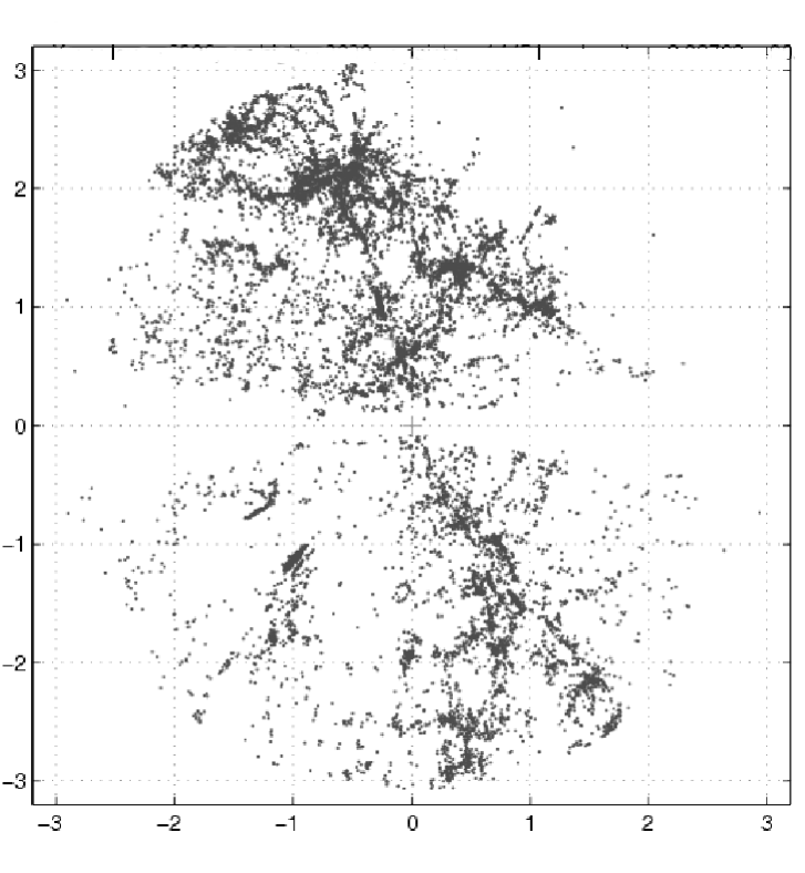
Figure 1.: The galaxy distribution in a slice 1600 km/s thick and 32000 km/s square. The Zone of Avoidance is clearly visible in the middle of the picture. Since the data are from different redshift surveys, some structures are well mapped, while other regions are not. Still there are regions from which there is no data at all.

3. Analysis of observations

As stated above, to properly analyze the observations general relativity has to be employed. The Einstein equations of general relativity are as follows:

$$G_{\alpha\beta}=\kappa T_{\alpha\beta}+\Lambda g_{\alpha\beta},$$ (1)

where $G_{\alpha\beta}$ is the Einstein tensor which describes the geometry of the space–time, $T_{\alpha\beta}$ is the energy–momentum tensor, $g_{\alpha\beta}$ is the metric, and $\Lambda$ is the cosmological constant. The Einstein equations state that there is a correspondence between the geometry of the space–time and matter distribution in the space–time. In general, these equations are a set of 10 partial differential equations, which are very hard to solve even numerically. However, if some symmetries are assumed, these equations can be solved analytically. The most popular assumption is that the space is homogeneous. However, because of homogeneity one cannot describe the process of structure formation. One of the alternatives is to employ a perturbation theory, such as the linear approach. However, structure formation is a very non–linear process (Bolejko 2006a; 2006b) hence the linear approach is inadequate. Another alternative is N–body simulation. The N–body simulation describes the evolution of a large amount of particles which interact gravitationally. However, the interactions between particles are described by Newtonian mechanics, and in the Newtonian mechanics matter does not affect light propagation. Hence within the N–body simulations it is impossible to estimate the influence of matter distribution on light propagation. In general relativity the situation is different, the geometry defined by matter distribution determines along which paths the light will propagate. Thus to trace light propagation and estimate the influence of cosmic structures on light propagation one has to use an exact solution of Einstein’s equations. But there are no exact solutions which would fully describe such a complicated system as our Universe. To describe the structure formation one has to focus on small scales, where one can employ models suitable for this purpose. For evolution of single structures (such as clusters or voids) the Lemaître–Tolman model (Lemaître 1933, Tolman 1934) can be used, and for evolution of double structures (a void and an adjourning cluster) the quasispherical Szekeres model can be employed. The Szekeres model represents a time–dependent mass dipole superposed on a monopole. So it is suitable for modelling double structures. The Szekeres model also makes it possible to examine interactions between the considered structures.

4. Szekeres model

For our purpose it is convenient to use a coordinate system different from that in which Szekeres (1975a) originally found his solution. The metric is of the following form (Hellaby & Krasiński 2002):

$$ds^{2}=c^{2}dt^{2}-\frac{(\Phi^{\prime}-\Phi\frac{\textstyle E^{\prime}}{\textstyle E})^{2}}{(\varepsilon-k)}dr^{2}-\Phi^{2}\frac{(dp^{2}+dq^{2})}{E^{2}},$$ (2)

where ${}^{\prime}\equiv\partial/\partial r$, $\varepsilon=\pm 1,0$ and $k=k(r)\leq\varepsilon$ is an arbitrary function of $r$.

The function $E$ is given by:

$$E(r,p,q)=\frac{1}{2S}(p^{2}+q^{2})-\frac{P}{S}p-\frac{Q}{S}q+C,$$ (3)

where the functions $S=S(r)$, $P=P(r)$, $Q=Q(r)$, and $C=C(r)$ satisfy the relation:

$$C=\frac{P^{2}}{2S}+\frac{Q^{2}}{2S}+\frac{S}{2}\varepsilon,~{}~{}~{}~{}~{}~{}~{}~{}~{}\varepsilon=0,\pm 1,$$ (4)

but are otherwise arbitrary.

As can be seen from (2), only $\varepsilon=+1$ allows the model to have all three FLRW limits (hyperbolic, flat, and spherical). This follows from the requirement of the Lorentzian signature of the metric (2). As we are interested in the Friedmann limit of our model, i.e. we expect it becomes a homogeneous Friedmann model at a large distance from the origin, we will focus only on the $\varepsilon=1$ case. The $\varepsilon=1$ case is called the quasispherical Szekeres model.

The Einstein equations reduce to the following two:

$$\frac{1}{c^{2}}\dot{\Phi}^{2}=\frac{2M}{\Phi}-k+\frac{1}{3}\Lambda\Phi^{2},$$ (5)

$$\kappa\rho c^{2}=\frac{2M^{\prime}-6ME^{\prime}/E}{\Phi^{2}(\Phi^{\prime}-\Phi E^{\prime}/E)}.$$ (6)

where $\dot{}\equiv\partial/\partial t$, $\rho$ is matter density, and $\kappa=8\pi G/c^{4}$.

In the Newtonian limit $c^{2}M(r)/G$ is equal to the mass inside the shell of radial coordinate $r$. However, it is not an integrated rest mass but the active gravitational mass that generates the gravitational field. By analogy with the Newtonian energy conservation equation, eq. (5) shows that the function $(-k/2)$ represents the energy per unit mass of the particles in the shells of matter at constant $r$. On the other hand, by analogy with the Friedman equation, and from the metric (2), the function $k$ determines the geometry of the spatial sections $t=$const. However, since $k$ is a function of the radial coordinate, the geometry of the space is now position dependent.

Eq. (5) can be integrated:

$$\int\limits_{0}^{\Phi}\frac{{\rm d}\tilde{\Phi}}{\sqrt{\frac{2M}{\tilde{\Phi}}-k+\frac{1}{3}\Lambda\Phi^{2}}}=ct-ct_{B},$$ (7)

where $t_{B}=t_{B}(r)$ appears as an integration constant, and is an arbitrary function of $r$. This means that the Big Bang is not a single event as in the Friedmann models, but occurs at different times for different distances from the origin.

As can be seen, the Szekeres model is specified by 6 functions. However, by a choice of the coordinates, the number of independent functions can be reduced to 5.

The Szekeres model is known to have no symmetry (Bonnor, Sulaiman, & Tomimura 1977). It is of great flexibility and wide application in cosmology (Bonnor & Tomimura 1976), and in astrophysics (Szekeres 1975b; Hellaby & Krasiński 2002), and still it can be used as a model of many astronomical phenomena. This paper aims to present the application of the quasispherical Szekeres model to the process of structure formation.

5. The Algorithm

Since the quasispherical Szekeres model represents a time–dependent mass dipole superposed on a monopole, we will employ this model to describe the evolution of a void and an adjourning galaxy supercluster. Below the algorithm of the model’s specification and its evolution is presented.

5.1. The model setup

To specify the model we need to know 5 functions. Let three out of these five unknown functions be $P(r),Q(r),S(r)$. These function are assumed to be of the following form:

$$S = 140,$$

$$P = 0,$$

$$Q = -113\ln(1+r).$$ (8)

The next two functions can be any two of the set $\{t_{B}(r),M(r),k(r)\}$, or of any other combination of functions, from which these can be calculated. The function $M(r)$ describes the active gravitational mass inside the $t=$ const, $r=$ const sphere. Let us take the mass distribution as presented in Fig. 2. Fig. 2 presents not the $M(r)$ function itself, but $Mc^{2}/G$ (see a comment after eq. (6)). Since the void is placed at the origin, the mass of the model in Fig. 2 is below the background mass, however, it is compensated by more dense regions, and at the distance of about $30$ Mpc the mass distribution becomes as in the homogeneous background.

To define the model we need one more function. Let us assume that the bang time function, $t_{B}(r)$, is constant and equal to zero. Then from eq. (7) the function $k(z)$ can be calculated. The LHS of eq. (7) was calculated using the 64–points Gauss–Legendre quadrature. The value of $t$ on the RHS of eq. (7) was assumed to be the present instant. Then the function $k$ was calculated by the bisection method.

Figure 2.: The mass distribution within the homogeneous background (BG) and in the Szekeres model (SZ).

5.2. Evolutionary code

As can be seen from eqs. (6), (3), and (4), to calculate the density distribution for any instant $t_{i}$, one needs to know 5 functions: $M(r),S(r),Q(r),P(r)$, and $\Phi(t_{i},r)$. Using these functions the density distribution of the present day structures can be calculated (see Sec. 6). Then, the evolution of the system can be traced back in time. The density distribution depends on time only via the function $\Phi(t,r)$ and its derivative. The value of $\Phi(t,r)$ for any instant can be calculated by solving the differential equation (5). In most cases, as in this paper, this equation can be solved only numerically. To solve this equation one needs to know the initial conditions: $\Phi(t_{0},r)$, the functions $M(r)$, $k(r)$, and the value of $\Lambda$. This equation was solved numerically using the fourth–order Runge–Kutt method. Knowing the value of $\Phi(t,r)$ for any instant the density distribution can be calculated as described above.

6. Model of cosmic structures

This section presets the evolution of the present–day void and the adjourning galaxy supercluster in the expanding Universe. Far away from the origin, density and velocity distributions tend to the values that they would have in a homogeneous Friedmann model. Fig. 3 presents the present–day density distribution of the considered structure. On the left side of Fig. 3 the schematic cross–sections are presented, on the right side density distributions on these cross–sections are presented. As can be seen, at large distance from the origin the density distribution is homogeneous and as the distance gets smaller the structure begins to appear. At the equator the structure is most visible. The density distribution on this equatorial cross–section (Fig. 3, at the bottom) is also presented at the top of Fig. 4. Fig. 4 depicts the colour coded (left side) density distributions. On the right side of Fig. 4 the density profiles are plotted. As can be seen the density distributions within these structures are consistent with the observational data presented in Sec. 2.

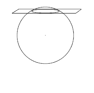
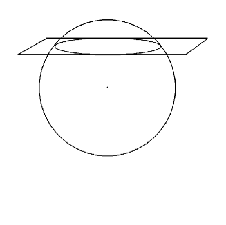
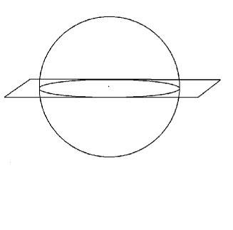
Figure 3.: Density distribution of the considered structure. Left side figures present the schematic cross–sections through the modeled region. Pictures on the right side present the density distributions which correspond to these cross–sections. The density is presented in the background density units, i.e. $\rho(r,t)/\rho_{b}(t)$, where $\rho_{b}$ is density of the background model. For detailed description see Sec. 6.

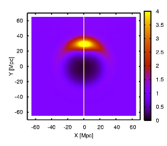
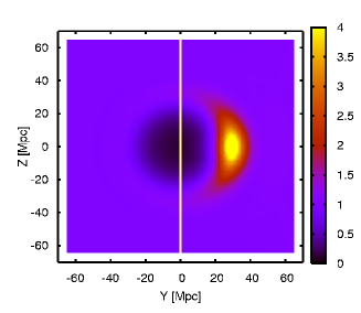
Figure 4.: Density distribution in the considered structure. Upper left panel presents colour coded density distribution of the equatorial cross section (see Fig. 3, bottom panels). Lower left panel presents the vertical cross–section of $X=0$, through the considered model. The yellow lines correspond to the density profiles, which are presented on the right side. For detailed description see Sec. 6.

6.1. Evolution of cosmic structures

This subsection discusses the evolution of the density profile presented in the upper right panel of Fig. 4. In Fig. 5 density profiles are plotted for different time instants. As can be seen in Fig. 5 the structure formation is a non–linear process. In the linear approach, during the evolution the shape of the initial fluctuation does not change. Only the amplitude changes. Moreover, in the linear approach the evolution of the density contrast does not depend on its sign. Here, as can be seen in Fig. 5., when the age of the Universe was 1 Gyr, the absolute value of the density contrast inside the void was larger than inside the cluster. When the age of the Universe was 5.5 Gyr, the absolute values of these density contrast were comparable. Since that instant the amplitude of the density contrast inside the cluster started to grow much faster than the absolute value of the amplitude inside the void. For detailed comparisons between the evolution in the linear approach and in the quasispherical Szekeres model see Bolejko (2006b).

Figure 5.: The density profile for diffrent time instants: a — 1 Gy after the Big Bang, b — 5.5 Gy, c — 10 Gy, d — present instant.

7. Futher applications of the Szekeres model

Light propagation within the Szekeres model can be investigated by calculating null geodesics. Systematic studies of this problem will provide insight in the following issues:

1. The impact of matter inhomogeneities on the luminosity distance.
   The studies of this issue within the Lemaître–Tolman model (Bolejko 2005) proved that realistic matter fluctuations can change the observed luminosity even by $\Delta m\approx 0.15$ mag. However, since the Lemaître–Tolman model assumes spherical symmetry, similar analysis in non–symmetrical models should be repeated.

2. Estimation of the age of the Universe.
   The estimated age of the Universe up to the last scattering moment within the Szekeres model and within the FLRW model is similar. This is due to homogeneous matter distribution. However, after the last scattering when matter inhomogeneities started to grow the results obtained within these two models might differ. For example the time that the light will need to propagate from regions of redshift $z\approx 1100$ is different in a homogeneous than in an inhomogeneous model. The difference is due to the interaction between the cosmic structures and the photons propagating through them. This difference can be estimated by employing the quasispherical Szekeres model.

3. The mass of galaxy clusters.
   The mass of a galaxy cluster can be estimated on the basis of dynamics of the observed galaxies. The observables of this method are: the angular distance from the center of the cluster, and the redshift. As mentioned above the distance to the point of redshift $z$ is different in various cosmological models. Also the angular distance from the center depends on the model. In most cases it is assumed that an angular distance is as in the Euclidean space — proportional to the physical distance. In general relativity, the path of light of the observed galaxy can be bent by the gravitational field of the cluster. The quasispherical Szekeres model can be used to estimate the impact of the inhomogeneous and non–symmetrical mass distribution on the calculated mass of observed cluster.

8. Conclusion

This paper presents the cosmological application of the quasispherical Szekeres model. This model is an exact solution of the Einstein field equations, which represents a time–dependent mass dipole superposed on a monopole. Therefore, the Szekeres model is suitable for modelling double structures such as voids and adjourning galaxy superclusters. The models based on the Szekeres solution have also one more advantage — they can be employed in solving problems of light propagation, which is impossible within the N–body simulations. The Szekeres model has a great, and so far unused, potential for applications in cosmology. It is not only suitable for studying the interactions between cosmic structures, but can also be used for estimation of the impact of matter inhomogeneities on light propagation. The Szekeres model is suitable for the investigation of following issues:

— the mass estimation based of the dynamics of galaxies,

— the luminosity of distant objects, such as high–redshift supernovae,

— the age of the Universe.

9. Acknowledgments

I would like to thank Andrzej Krasiński and Charles Hellaby for their valuable comments and discussions concerning the Szekeres model.

References

Bardelli, S., Zucca, E., Zamorani, G., Moscardini, L., & Scaramella, R. 2000, MNRAS, 312, 540

Bolejko, K. 2005, astro-ph/0512103

Bolejko, K. 2006a, MNRAS (to be published); pre-print: astro-ph/0503356

Bolejko, K. 2006b, Phys. Rev. D (to be published); pre-print: astro-ph/0604490

Bonnor, W. B., Sulaiman, A. H., & Tomimura, N. 1977, Gen. Relativ. Gravitation, 8, 549

Bonnor, W. B., & Tomimura, N. 1976, MNRAS, 175, 85

Hellaby, C., & Krasiński, A. 2002, Phys. Rev. D, 66, 084011

Hoyle, F., & Vogeley, M. S. 2004, ApJ, 607, 751

Hudson, M. J. 1993, MNRAS, 265, 43

Kolatt, T., Dekel, A., & Lahav, O. 1995, MNRAS, 275, 797

Lemaître, G. 1933, Ann. Soc. Sci. Bruxelles, A53, 51; reprinted in 1997, Gen. Relativ. Gravitation, 29, 641

Szekeres, P. 1975a, Commun. Math. Phys., 41, 55

Szekeres, P. 1975b, Phys. Rev. D12, 2941

Tolman, R. C. 1934, Proc. Nat. Acad. Sci. USA, 20, 169; reprinted in 1997, Gen. Relativ. Gravitation, 29, 935