X-ray Spectral Study of the Photoionized Stellar Wind in Vela X-1

Abstract

We present results from quantitative modeling and spectral analysis of the high mass X-ray binary system Vela X-1 obtained with the Chandra High Energy Transmission Grating Spectrometer. The observations cover three orbital phase ranges within a single binary orbit. The spectra exhibit emission lines from H-like and He-like ions driven by photoionization, as well as fluorescent emission lines from several elements in lower charge states. The properties of these X-ray lines are measured with the highest accuracy to date. In order to interpret and make full use of the high-quality data, we have developed a simulator, which calculates the ionization and thermal structure of a stellar wind photoionized by an X-ray source, and performs Monte Carlo simulations of X-ray photons propagating through the wind. The emergent spectra are then computed as a function of the viewing angle accurately accounting for photon transport in three dimensions including dynamics. From comparisons of the observed spectra with results from the simulator, we are able to find the ionization structure and the geometrical distribution of material in the stellar wind of Vela X-1 that can reproduce the observed spectral line intensities and continuum shapes at different orbital phases remarkably well. We find that the stellar wind profile can be represented by a CAK-model with a star mass loss rate of (1.5–2.0) $\times 10^{-6}M_{\sun}\mathrm{yr}^{-1}$, assuming a terminal velocity of 1100 km s^-1. It is found that a large fraction of X-ray emission lines from highly ionized ions are formed in the region between the neutron star and the companion star. We also find that the fluorescent X-ray lines must be produced in at least three distinct regions – (1) the extended stellar wind, (2) reflection off the stellar photosphere, and (3) in a distribution of dense material partially covering and possibly trailing the neutron star, which may be associated with an accretion wake. Finally, from detailed analysis of the emission line profiles, we demonstrate that the stellar wind dynamics is affected by X-ray photoionization.

1. Introduction

In a high mass X-ray binary (HMXB), a compact object, either a neutron star or a black hole, sweeps up material as it orbits through the stellar wind of a massive O- or B-type companion star. When the material is accreted onto the compact object, a fraction of its gravitational potential energy is converted into X-rays, which in turn ionizes and heats the surrounding stellar wind. X-ray photons from the compact object are reprocessed by the ionized material, resulting in discrete spectral features, which carry a wealth of information about the geometry and physical state of the material in the system. The compact object can, therefore, be used as a radiation source to probe the structure of the stellar wind to derive the physical parameters that characterize its nature.

Vela X-1 is the archetype HMXB consisting of a neutron star and a massive companion star, and as such it has been the most well-studied object in this class since its discovery. It is an eclipsing HMXB system containing a pulsar with a pulse period of 283 s (McClintock et al., 1976) and an orbital period of 8.964 days (Forman et al., 1973). The optical companion star, HD 77581, is a B0.5Ib supergiant (Brucato & Kristian, 1972; Hiltner, Werner & Osmer, 1972), which drives a stellar wind with a mass-loss rate in the range (1 – 7) $\times$ 10${}^{-6}~{}M_{\sun}$ yr^-1 (Hutchings, 1976; Dupree et al., 1980; Kallman & White, 1982; Sadakane et al., 1985; Sato et al., 1986). The terminal velocity of the stellar wind was determined to be 1100 km s^-1 from the P-Cygni profile of UV resonance lines (Prinja et al., 1990). Its average intrinsic X-ray luminosity is $\sim$ 10³⁶ erg s^-1, which is consistent with accretion of the stellar wind by the gravitational field of a neutron star.

The first attempt to model the global X-ray emission line spectrum of Vela X-1 was presented by Sako et al. (1999) using the CCD spectrum obtained with ASCA. They characterized the wind using a standard velocity profile of OB stars proposed by Castor, Abbott & Klein (1975) (CAK model). By adjusting the mass loss rate, they found a statistically acceptable fit to the ASCA spectrum. However, since the energy resolution of ASCA is not sufficiently high to resolve any of the emission lines predicted by the ionization model, the intensity measurement of each line is limited due to blending. In addition, since the expected X-ray line shifts and widths are much smaller than the width of the instrument response, they were not able to extract any information about the dynamics of the X-ray emitting gas.

The spectral resolution ($E/\Delta E$ $\sim$ 100–1000) of the transmission grating spectrometers on board Chandra have provided a detailed view of the emission line spectrum, including accurate measurements of line intensities and velocity profiles in a number of HMXBs (Vela X-1: Schulz et al. 2002, Goldstein et al. 2004; GX 301$-$2: Watanabe et al. 2003; Cyg X-3: Paerels et al. 2000; 4U 1700$-$37: Boroson et al. 2003). Schulz et al. (2002) present the first high-resolution X-ray spectrum of Vela X-1 observed during eclipse. They detect a narrow RRC from Ne X with an electron temperature of $\sim$ 10 eV, which implies that the stellar wind is indeed driven by photoionization. Goldstein et al. (2004) present the spectra of Vela X-1 observed during the three orbital phase ranges – eclipse, $\phi$ = 0.25, and $\phi$ = 0.50. They report the first detection of multiple emission lines at orbital phase $\phi$ = 0.5 and analyzed the spectral changes between the three orbital phases.

In this paper, we present a quantitative analysis of the X-ray spectra of Vela X-1 first presented by Goldstein et al. (2004) using the data obtained with Chandra High Energy Transmission Grating Spectrometer (HETGS) during three orbital phase ranges. We construct a simulator to compute the physical conditions of the surrounding gas for a given binary configuration, stellar wind parameters, and X-ray luminosity. Continuum photons that originate from the compact object interact with the atoms to produce emission lines and continua, which are propagated through the wind accounting for all relevant radiative transfer effects including line scattering/absorption, continuum absorption, and Compton scattering. The emerging spectra are calculated and compared with the observed orbital-phase-resolved spectra, which provide constraints on the global physical properties of the ionized stellar wind.

This paper is organized as follows. In § 2, we describe the Chandra observations and summarize the data reduction procedures. The reduced spectra are fitted using simple empirical models to extract the general properties of the stellar wind. In § 3, we provide a full description of the simulator, which is used to model the binary system and to calculate the resulting spectra as a function of the orbital phase. In § 4, we describe a self-consistent picture of the Vela X-1 system derived from the simulator in comparison to the data. We finally summarize our results in § 5.

2. Observations and Results

Vela X-1 was observed with the Chandra HETGS/ACIS-S during three different orbital phase ranges within a single binary orbit in February 2001 – (1) $\phi$ = 0.237–0.278, (2) $\phi$ = 0.481–0.522, and (3) $\phi$ = 0.980–0.093, hereafter referred to as phase 0.25, phase 0.50, and eclipse, respectively. The observation dates and exposure times are summarized in Table 1. A schematic drawing of the binary orbit and the phase ranges are shown in Fig. 1.

All of the data are processed using CIAO v2.3, and spectral analyses are performed using XSPEC. Since the zeroth order image was severely piled-up during phase 0.25 and phase 0.50, the locations of the zeroth order image were determined by finding the intersection of the dispersed events as well as the streak events, which are produced during CCD frame transfer. This gives us a zeroth order location that is accurate to within 0.1 pixels, which is much smaller than the instrument line response. The positive and negative spectral orders are inspected separately to check that systematic offsets do not exist. We then apply spatial filters for both the Medium Energy Grating (MEG) and the High Energy Grating (HEG) data, and subsequently use an order sorting mask by using the energy information obtained with ACIS-S. Only the first order events are used in our spectral analyses. The background events are estimated from the adjacent region to the dispersed event region and are found to contribute at most 5 % for the eclipse data and 3% for the phase 0.25 and phase 0.50 data. The background is subtracted in the spectral analyses.

2.1. Continuum Emission

Figure 2 shows the HEG spectra for the three orbital phases. X-rays emitted from the neutron star are directly observed during phase 0.25 and phase 0.50 as continuum spectra. As expected from the geometry of the binary system, the spectrum taken in eclipse is dominated by line emission and scattered components. In order to parameterize the properties of the continuum, we fit the spectra with a photo-absorbed power-law function. Since the spectrum of phase 0.25 is affected less by absorption, we leave both the hydrogen column density and the photon index as free parameters in the fit. On the other hand, for phase 0.5, we fix the photon index to the value obtained from phase 0.25 and calculate the absorption. We assume that the chemical abundance of metals in the absorbing material is 0.75 times the cosmic abundance (Feldman, 1992), which is known to be a representative value for typical OB-stars (Bord et al., 1976). The derived parameters from the spectral fits are listed in Table 2. The best-fit models are superimposed on the spectra in Fig. 2. The absorption-corrected luminosity is determined to be identical for observations in phase 0.25 and in phase 0.50 and corresponds to 1.6 $\times$ 10³⁶ erg s^-1 in the 0.5–10 keV range, assuming a distance of 1.9 kpc (Sadakane et al., 1985).

2.2. Line Emission

A large number of emission lines are clearly detected in the spectra of phase 0.50 and eclipse as shown in Fig. 3 and Fig. 4. Emission lines from H-like and He-like S, Si, Mg and Ne can be seen, in addition to fluorescent lines from Fe, Ca, S, and Si ions in lower charge states. We note that emission lines from the same ions are detected in the spectra of both phase 0.50 and eclipse.

In Fig. 5, we show the three spectra in a narrow energy range of $E=1.70-2.05$ keV, which contains the K$\alpha$ transitions of Si. An intense Ly$\alpha$ line from H-like Si and fully-resolved He-like triplet lines are clearly seen in the phase 0.50 and eclipse spectra. At slightly lower energy, a spectacular complex of emission lines are also detected, which we identify as K$\alpha$ fluorescent lines from Si in lower charge states. In the phase 0.5 spectrum, the near-neutral lines (Si II – Si VI) are blended at $E\sim 1.74$ keV, and a series of lines above this energy are resolved into those from Si VII – Si XI. This implies that the stellar wind in this system contains an extremely wide range in ionization parameter. The eclipse spectrum also shows a similar structure, but with much lower intensities.

The centroid of energies, the widths and the intensities of each line are determined by representing them with single gaussian components. In the spectral fittings, we use the Poisson likelihood statistics, instead of the $\chi^{2}$ statistics, because the numbers of photons in some of the bins in the spectra are small. The derived parameters for phase 0.50 and eclipse are listed in Table 3 and Table 4, respectively. We also show list in Table 5 the line intensity ratios between phase 0.50 and eclipse for the H- and He-like lines that are detected with a statistical significance of more than 5 $\sigma$. The H-like lines are brighter during phase 0.5 by a factor of 8–10 compared to during eclipse, and similarly the He-like lines are 4–7 times stronger.

The resolving power of the HETGS allows us to measure Doppler shifts to an accuracy of $\sim$ 100 km s^-1. Figure 6 compares the line profiles of Si Ly$\alpha$ and Mg Ly$\alpha$ between phase 0.50 and eclipse. The offset in the line center energies are clearly seen. We measure the velocity shifts of all of the K$\alpha$ lines of H-like and He-like ions, which are plotted in Fig. 7. Though some fluctuations are seen, there is a general trend that the lines are blue-shifted during phase 0.50, and they are red-shifted during eclipse as expected from an outflowing wind irradiated by an X-ray source. The velocity shifts have values in the range in $\Delta v~{}\sim$ 300–600 km s^-1 (Table 5 and widths of $\sigma\lesssim 300$ km s^-1.

Radiative recombination continuum (RRC) is detected clearly from H-like Ne. We fitted the RRC spectra using the “redge” model in XSPEC. The electron temperatures are determined to be $kT_{e}=7.4_{-1.3}^{+1.6}$ eV and $kT_{e}=6.6_{-1.8}^{+2.5}$ eV during phase 0.50 and eclipse, respectively.

Iron K$\alpha$ fluorescent lines are detected in all three orbital phases. The profiles of these lines are shown in Fig. 8. The parameters derived from the spectral fits with single gaussian models are listed in Table 6. The equivalent width of the iron K$\alpha$ line is measured to be 116 eV and 51 eV for phases 0.50 and 0.25, respectively. During eclipse, a high equivalent width of 844 eV is observed. As shown in Fig. 8, there is an indication of a Compton shoulder in the iron K$\alpha$ line at phase 0.50.

2.3. Summary of Results and their Implications

Some general global properties of the circumsource medium can be deduced from the results of the simple fitting procedures described in § 2.1 and § 2.2.

The continuum from the neutron star is highly absorbed during phase 0.5 whereas the absorption column density is reduced during phase 0.25. This implies that there is an absorber located behind the neutron star as viewed from the companion star. The average continuum intensities are nearly identical during the two phase ranges. The presence of strong soft X-ray lines during phase 0.5, however, suggests that this absorber is localized and does not cover the X-ray emission line regions, which most likely extend beyond the size of the absorber.

The emission lines during phase 0.50 is approximately an order of magnitude brighter than those during eclipse. This indicates that a significant fraction of the X-ray line emission is produced in a region between the neutron star and the companion star, which is occulted during eclipse. The velocity shifts and widths provide additional constraints on the properties of the emission region. The measured Doppler shifts of $\lesssim 500$ km s^-1 are much smaller than the terminal velocity of Vela X-1 ($v_{\infty}=1100$ km s^-1; Prinja et al. 1990). For a Castor, Abbott & Klein (1975) stellar wind velocity profile of isolated OB stars, this velocity is achieved at only 0.25 stellar radii from the photosphere. The Doppler broadening of emission lines is also small ($\lesssim 300$ km s^-1). These observational results shows that the emission site of lines from highly ionized ions is distributed on a plane between the neutron star and the companion star, with most of the emission coming from near the line of centers.

Finally, the detection of a narrow radiative recombination continuum from H-like Ne during phase 0.5 and in eclipse with electron temperatures of 6–8 eV provides direct evidence that the emission lines from highly ionized gas in Vela X-1 are driven through photoionization. Other possible sources of mechanical heating are, therefore, not important in characterizing the ionization structure of at least the highly-ionized regions of the stellar wind.

3. Outline of the Simulator

3.1. Modeling of Photoionized Plasma

The X-ray emission lines detected from Vela X-1 can be interpreted as due to emission from a gas photoionized by the continuum radiation from the neutron star. When line photons are created through recombination cascades following photoionization, they interact with the surrounding gas as they propagate out of the binary system, and this is controlled by the ionization structure and the density distribution of the gas in the stellar wind. Therefore, by investigating the properties of the emission lines, we can infer the physical conditions, geometrical distribution, and the velocity structure of the wind.

In order to compute the ionization structure and to reproduce the wealth of information provided by the high-resolution HETGS spectra, it is necessary to model the emission using realistic physical models of the stellar wind in a binary system. We have developed three-dimensional Monte Carlo radiative transfer code to simulate the interactions of X-rays with the particles in the stellar wind.

Our simulation code consists of two main components:

(1)

Calculation of the ionization structure.

(2)

Monte Carlo simulation for radiative transfer.

In part (1), we construct a map of the ion abundance and temperature in the stellar wind. In part (2), we use the results from part (1) and propagate X-ray photons from the neutron star out of the binary system. The simulation is performed on a three-dimensional grid of cells, which is capable of treating complex geometries. Radiative transfer effects that are important for highly ionized media are included. The medium is allowed to have arbitrary velocities, and Lorentz transformations are performed between the cells, which is necessary to calculate the correct output line profiles. Our detailed procedures are described in the following subsections.

3.2. Calculation of the Distribution of Ionization Degree

The ionization balance and electron temperature are determined primarily by the particle density and the local flux and spectral shape of the ionizing X-rays. We compute the three-dimensional ionization structure by first dividing the binary system into square cells of equal size. Since the system is assumed to be cylindrically symmetric along the line of centers, we compute the ion fractions and temperatures on a two-dimensional grid as shown in Fig. 10. Each cell is $4\times 10^{11}$ cm along the side and the system consists of $61\times 31$ cells.

The density structure around the companion star is specified from the velocity profile determined from the UV observation and an assumed mass-loss rate, which is treated as a free parameter. This assigns a particle density to each of the cells. The intrinsic luminosity and spectrum shape of the X-ray source as determined from the observed spectrum are then placed in the cell where the neutron star is located. The ion fractions and the electron temperatures of the cells immediately surrounding the neutron star are computed using this initial continuum shape as the input ionizing radiation field. The computation moves outwards to the next layer of cells, this time, using a different continuum shape, which accounts for absorption by the inner cells. This procedure continues until the outermost cells are reached. We have use the XSTAR program to calculate the ion fractions H, He, C, N, O, Ne, Mg, Si, S, Ar, Ca, and Fe, and the electron temperature in each cell. A flowchart of the procedures is shown in Fig. 9.

This procedure ignores the diffuse radiation field as the source of additional ionization, which is a small contributor to the total photoionization rate at least for the ions observed in our spectra. A more accurate treatment of this effect might involve an iterative scheme, which is not necessary for our present analysis, but may be important for extremely optically thick media.

3.3. Monte Carlo Calculation of the X-ray Emission from Photoionization Equilibrium State

The map of the ion fractions calculated by the method described in the previous subsection assures equilibrium between photoionization and recombination. We then use this ionization structure to propagate again the continuum photons originating from the neutron star to compute the emitted X-ray spectra as a function of the orbital phase. This is done by accounting for radiative transfer effects in detail and using Monte Carlo methods as described below.

The cells are set up somewhat differently from those used in the calculation of the ionization structure. The cells sizes are chosen so that each of them are not optically thick to the strongest resonance lines. Smaller cells are required near the companion star where both the density and density gradient are high, and we choose cubic cell sizes of $4\times 10^{11}$ cm on each side. The cells are increased in size outwards and the outermost cells of the simulation space are larger by a factor of 7.5 compared to the inner ones as shown in Fig. 10. We start the Monte Carlo simulation with a photon at the position of the central neutron star. The photon energy is drawn from the observed power-law spectral energy distribution and is initially given a random direction. This photon is then traced through the cells and interacts with the ions in the stellar wind, which then generates a secondary photon through radiative recombination, radiative transitions, and fluorescent emission. All of the photons including those from the central continuum and subsequent line photons produced by interactions are propagated until they either completely escape the simulation space or are destroyed by one of the physical processes described below. The emergent photons are then selected depending on the viewing angle of the system, and are finally histogrammed to produce a spectrum.

When a photon interacts with a particle, one of three physical processes is allowed to occur: (1) photoionization, (2) photoexcitation, and (3) Compton scattering. For a given photon energy, the absorption and scattering cross sections and hence the optical depths are calculated for each ion within a given cell. Interaction probabilities are then assigned to each possible process and are drawn via Monte Carlo. Although process (1) produces a free electron and process (3) changes the energy of a free electron, we do not trace them in our simulations, but instead simply assume that they are thermalized before any further interaction takes place.

As mentioned earlier, we assume that photoionization equilibrium is established locally everywhere in the plasma. Therefore, photoionization of H- or He-like ions is always followed by radiative recombination and radiative cascades to the ground level. For ions of lower charge states, K-shell photoionization is followed by either fluorescent emission or Auger decay. After photoexcitation, the ion in an excited state produces one or more photons in the downward radiative transitions that eventually lead to the ground level. By the combination of the photoexcitation and the downward radiative transitions, the resonance scattering of the lines is incorporated in the Monte Carlo simulation.

For the H-like and He-like ions, we compute all of the atomic quantities with the Flexible Atomic Code (FAC). This includes energy levels, oscillator strengths, radiative decay rates, photoionization cross sections from all levels between the ground state up to $n=10$. Radiative recombination rates onto each of levels as a function of the electron temperature are also computed from the photoionization cross sections using the Milne relation. Collisional transfers and UV photoexcitations in the He-like ions are not included in the current version of the code.

Photoionization of ions with three or more electrons de-excites by either an emission of fluorescent photon or ejection of one or more Auger electrons. The K-shell photoionization cross sections are computed using the fitting formulae provided by Band et al. (1990), which roughly accounts for the change in the K-edge energy and cross section as functions of the charge state. The fluorescence yields and K$\alpha$ energies, however, are assumed to be fixed for a given element and their values are adopted from (Larkins, 1977) and (Salem, Panossian & Krause, 1974; Krause, 1979), respectively, for neutral atoms. We also do not account for K-shell ionization of Li-like ions, which can lead to the production of the He-like forbidden line. We use L-shell cross sections from EPDL97 , which is also valid for neutral atoms. The L₁, L₂ and L₃-shell cross sections are taken into account for the ions with three, five, and six electrons, respectively. Finally, we do not include L-shell fluorescent emission, since the yields are typically much smaller compared to the K-shell fluorescence yields.

We consider Compton scattering only by free electrons, which is an excellent approximation for highly ionized media. The differential cross section is given by the the Klein-Nishina formula and the electrons velocities are drawn from a Maxwellian distribution with the local electron temperature.

Doppler shifts due to the motion of the stellar wind are accounted for in all of the processes. When a photon enters a cell, the cross sections are calculated for the photon energy in the co-moving frame and Lorentz transformed back into the rest frame. The Doppler shifts could affect the line strength through the resonance line scattering. A velocity gradient can change the ratio of the line escape. In this Monte Carlo simulation, such Doppler effects on the lines are included, though the reproducibility of the velocity gradient is limited by the geometry cell size.

4. The Physical Properties of the Stellar Wind in Vela X-1

4.1. Structure of the Stellar Wind

We first search for the value of the mass loss rate that reproduces the observed line intensities as a function of the orbital phase. We assume that the velocity structure of the stellar wind is represented by a generalized CAK (Castor, Abbott & Klein, 1975) profile:

$$v(r)=v_{\infty}\left(1-\frac{R_{*}}{r}\right)^{\beta},$$ (1)

where $r$ is the distance from the center of the star, $R_{*}$ is the stellar radius, and $v_{\infty}$ is the terminal velocity. We use a terminal velocity of 1100 km s^-1 as determined from UV observations of Vela X-1 (Prinja et al., 1990) and fix the value of $\beta$ to 0.80 (Pauldrach, Puls & Kudritzki, 1986).

For a given velocity profile and a mass loss rate $\dot{M}_{*}$, the wind density can be calculated by applying the equation of mass continuity assuming spherical symmetry,

$$n(r)=\frac{\dot{M}_{*}}{4\pi\mu m_{p}v(r)r^{2}},$$ (2)

where $\mu$ is the gas mass per hydrogen atom, which is $\sim 1.3$ for cosmic chemical abundances. This specifies the density at each point in the stellar wind, and the observed X-ray luminosity can be used to obtain a map of the ionization parameter.

The binary system parameters used in the simulations are listed in Table 7. The X-ray radiation field from the neutron star is modeled based on the parameter determined from the fits to the observed spectra at phase 0.25 and phase 0.5. Since no change in the average intrinsic luminosity is observed between these phases, we assume that the luminosity remains unchanged during the eclipse phase as well. The power-law spectrum with a photon index $\Gamma=1$ is assumed to extend up to 20 keV, which is the cut-off energy detected by previous hard X-ray observations with Ginga (Makishima et al., 1999) and RXTE (Kreykenbohm et al., 1999). The corresponding 0.5–20 keV luminosity is 3.5 $\times$ 10³⁶ erg s^-1. In the following subsection, we discuss the results of our simulation for mass loss rates of 5.0 $\times$ 10^-7, 1.0 $\times$ 10^-6, 1.5 $\times$ 10^-6, and 2.0 $\times$ 10^-6 $M_{\sun}$ yr^-1.

4.2. The Ionization Structure

Figure 12 shows maps of the H-like ion fraction of Si $f_{\mathrm{SiH-like}}$ at three different values for the mass loss rate. At a mass loss rate of 5.0 $\times$ 10^-7 $M_{\sun}$ yr^-1, the concentration of H-like Si is highest near the mid-plane of the binary system as shown on the left panel of Fig. 12. As the mass loss rate is increased, the density everywhere in the wind is also increased. For a fixed ionization parameter, the distance to the neutron star has to be reduced, so the region moves closer towards the neutron star as shown in the middle and right panels of Fig. 12. Multiplying the maps in Fig. 12 by the local density of the stellar winds gives the maps in Fig. 12. These show the absolute abundances of H-like Si $n_{\mathrm{SiH-like}}$ and the region where the X-ray photons of the emission line are produced.

According to these simulations, a large fraction of emission lines from highly ionized ions such as H-like Si are produced in the region between the companion star and the neutron star. This is the region that is obscured by the companion star during eclipse. It turns out that the mass loss rate is sensitive to the ratio of line fluxes between phase 0.5 and eclipse, because the size of the region becomes larger when we increase the mass loss rate. If a different value for the terminal velocity is assumed, the mass loss rate will differ such that the quantity $\dot{M}_{*}/v_{\infty}$ remains fixed.

4.3. Estimate of the Mass Loss Rate

The simulations are run for the various values of the mass loss rate. In order to calculate the observed spectra at different orbital phases, we designate the direction of the outgoing photon by the angle $\theta$ that the momentum vector makes relative to the line of centers (see, Fig. 13). The phase 0.5 spectrum is constructed from the outgoing photons with $\theta<10\arcdeg$ and the eclipse spectrum is made from photons with $170\arcdeg<\theta<180\arcdeg$. In this calculation, photons directly coming from the neutron star are neglected since only the emission lines and scattered components are of interest.

Although many emission lines are resolved in the Chandra spectra, we use only the Si XIV Ly$\alpha$ line to estimate the mass loss rate. This line is one of the brightest lines observed in the data. Since the energy of this line is sufficiently high, the uncertainties associated with foreground absorption is lower than the low energy lines. At this energy, an uncertainty of 1 $\times$ 10²¹ cm^-2 in $N_{\mathrm{H}}$, corresponds to only a $\sim 5$% uncertainty in the Ly$\alpha$ intensity.

The simulated intensity ratio of the Si XIV Ly$\alpha$ lin between phase 0.5 and eclipse as a function of the mass loss rate is shown in Fig. 14. The errors associated with these points are due to the finite number of photons generated in the simulation. The horizontal lines indicate the $1\sigma$ range in the observed value. As mentioned earlier in § 4.2, the ratio becomes larger as the mass loss rate is increased. The intensities of the Si Ly$\alpha$ in the phase 0.5 and in the eclipse are shown in Fig. 15. From these three plots in Fig. 14 and Fig. 15, the mass loss rate is estimated to be (1.5–2.0) $\times 10^{-6}M_{\sun}\mathrm{yr}^{-1}$.

The estimated mass loss rate of the stellar wind is consistent with the observed X-ray continuum luminosity. The mass accreting rate onto the neutron star $\dot{M}_{acc}$ is given by

$$\dot{M}_{acc}=\frac{\dot{M}_{*}R_{acc}^{2}}{4D^{2}},$$ (3)

where $\dot{M}_{*}$ is the mass loss rate of the stellar wind, and $D$ is the distance of the neutron star from the center of the OB star. $R_{acc}$ is the accretion radius express as:

$$R_{acc}=\frac{2GM_{ns}}{v_{rel}^{2}},$$ (4)

where $v_{rel}$ is the relative velocity of the neutron star and the stellar wind. The gravitational energy of the accreting material is converted into X-rays. The X-ray luminosity resulting from this accretion will simply be the rate at which gravitational energy is released:

$$L_{x}=\frac{GM_{ns}\dot{M}_{acc}}{R_{ns}}=\frac{\left(GM_{ns}\right)^{3}\dot{M}_{*}}{R_{ns}v_{rel}^{4}D^{2}}$$ (5)

where it is assumed that most of this energy is liberated near the neutron star surface (of radius $R_{ns}$). If $M_{ns}=1.7M_{\sun}$ (van Paradijs et al., 1977; Barziv et al., 2001), $R_{ns}=10$ km, $v_{rel}=640$ km s^-1 ($v_{wind}=570$ km s^-1, $v_{orbit}=300$ km s^-1), $D=53.4R_{\sun}$ and $\dot{M}_{*}=1.5\times 10^{-6}M_{\sun}\mathrm{yr}^{-1}$ are applied, an X-ray luminosity of $L_{X}=4.7\times 10^{36}$ erg s^-1 is obtained, which agrees with the observed luminosity of 3.5 $\times$ 10³⁶ erg s^-1 within a factor of 2.

From the eclipse spectrum obtained by ASCA, Sako et al. (1999) estimated that the mass loss rate associated with the highly ionized component of the stellar wind is $2.7\times 10^{-7}M_{\sun}\mathrm{yr}^{-1}$, which is a factor of 5–8 lower than the current estimate. The lower mass loss rate was derived most likely because only the eclipse data was used. As the mass loss rate is increased, the intensities of the emission lines from highly ionized ions become higher. When the mass loss rate is increased further, the photoionized region is occulted by the companion star and the intensities of the emission lines during the eclipse phase become lower. This tendency for the Si XIV is shown in Fig. 15 (left). There were two solutions for the eclipse spectrum, and, Sako et al. (1999) found the solution of the lower mass rate. However, we note that the intensity of emission lines in the phase 0.50 obtained with Chandra cannot be explained with such a lower mass loss rate. We, therefore, have concluded the higher mass loss rate of 1.5–2.0 $\times 10^{-6}M_{\sun}\mathrm{yr}^{-1}$. These measurements were probably not possible with the moderate spectral resolution of the instruments on board ASCA.

4.4. The Global X-ray Spectrum

Adopting a mass loss rate of 1.5 $\times$ 10^-6 $M_{\sun}$ yr^-1 estimated from the Si XIV line, we use the results of the Monte Carlo simulation to generate broadband spectra including both the continuum and emission lines from other ionic species for the three orbital phases observed with the HETGS. Photons with outgoing momenta in the $\theta$ ranges of 0°–10°, 85°–95°, and 170°–180° are used for the phase 0.50, phase 0.25, and eclipse model spectra, respectively.

Figure 16 shows both the observed spectra above $\sim 2$ keV and the simulated model spectra convolved through the response of the HETGS. The simulated spectra are multiplied by the effects of inter-stellar absorption ($N_{\mathrm{H}}=6\times 10^{21}$ cm^-2) in addition to intrinsic absorption by the stellar wind, which depends on the observed binary phase. This matches the observed continuum shape remarkably well at both phases 0.25 and eclipse. At phase 0.5, however, the observed column density of $N_{\mathrm{H}}=1.85\times 10^{23}$ cm^-2 is in excess of the Galactic plus stellar wind by an amount $N_{\mathrm{H}}=1.7\times 10^{23}$ cm^-2. We apply this additional absorption component to the continuum emission to match the data.

The simulated spectra at the three orbital phases are shown in Fig. 17. The observed emission line spectra in comparison with the simulations are shown in Fig. 18. The lack of obvious discrete spectral features at phase 0.25 is consistent with the model predictions, which show P-Cygni lines with comparable emission and absorption equivalent widths and are therefore washed out after convolution with the spectral response. We note that the additional absorption component observed at phase 0.50 does not appear to be affecting the emission lines, which implies that this absorber is localized to a small region along the line of centers and in front of the neutron star at phase 0.5. The simulated spectra match fairly well the emission lines from H-like and He-like ions, as well as the radiative recombination continuum emission. The ratios of simulated line intensities to the observed ones are plotted for those lines that are detected at greater than 5 $\sigma$ in Fig. 19. All of the simulated line intensities are within the observed values to within a factor of $\sim 3$. One of the uncertainties of the line intensities is the absorption, and it is difficult to derive the line intensities precisely by unfolding the absorption effect. In the simulation, the effects of inter-stellar absorption ($N_{\mathrm{H}}=6\times 10^{21}$ cm^-2) and intrinsic absorption by the stellar wind ($N_{\mathrm{H}}\sim 1.5\times 10^{22}$ cm^-2) are assumed. If there is an additional absorption of 10% of the assumed value, the intensities of Ne lines are reduced to $\sim$ 50%. Additionally, the absorption cross sections are very sensitive to the ionization degree of the absorption matter.

4.5. The Iron K$\alpha$ Line Complex

Fluorescence emission lines, in particular the bright iron line complex, provide information about the distribution of cold material around the X-ray source. Figure 8 shows the iron K$\alpha$ line spectrum at the three orbital phases, together with the models obtained from the simulations described in the previous subsection. During eclipse, the iron K$\alpha$ line intensity calculated from the simulation is consistent with the observed one. Therefore, it seems likely that the iron K$\alpha$ line observed in eclipse is produced in the cool regions of the extended stellar wind. On the other hand, we find that this same model cannot explain the observed intensity of the K$\alpha$ line in the other two phases. The equivalent widths from the simulations are only 4 eV and 11 eV for phases 0.25 and 0.50, whereas the observed values are 51 eV and 116 eV, respectively.

As an obvious source of additional line production regions, we first consider the surface of the companion star. Using Monte Carlo simulations and adopting the geometrical parameters listed in Table 7, we obtain reflected iron K$\alpha$ equivalent widths of 29 eV and 65 eV during phase 0.25 and phase 0.50, respectively, assuming that the metal abundance of the companion star is also 0.75 times the cosmic value. Therefore, the stellar wind and the companion surface combined yield equivalent widths of 33 eV (phase 0.25) and 76 eV (phase 0.50). The observed values are still in excess these values by 18 eV and 40 eV at phase 0.25 and 0.5, respectively.

We note the presence of excess absorption of $N_{\mathrm{H}}$ = 1.7 $\times$ 10²³ cm^-2 observed during phase 0.5 relative to that at phase 0.25. This suggests that a distribution of cold localized material lies along the line of centers somewhere behind the neutron star as viewed from the companion. We therefore expect that at least some amount of Fe-K line photons are produced in this cloud. This has already been pointed out by Inoue (1985) using the Tenma data.

In order to estimate the contribution of the cloud to the iron line flux, we have performed a Monte Carlo simulation of a partially covered cloud irradiated by an X-ray source. The geometrical configuration is shown schematically in Fig. 20. The thickness of the cloud is assumed to be $N_{\mathrm{H}}=1.7\times 10^{23}$ cm^-2 and we assume a uniform density. The cloud is assumed to be neutral and its metal abundance is set to 0.75 cosmic. The resulting emission spectra as functions of the orbital phase with the solid angle as the free parameter are computed through the same procedures as in the previous simulations, and the simulated Fe K$\alpha$ line equivalent widths are measured at the three orbital phases.

Figure 21 shows the relation between the solid angle subtended by the cloud and the iron line equivalent width. As can be seen from this figure, the missing equivalent widths outside of eclipse (18 eV at phase 0.25 and 40 eV at phase 0.50) can be explained if the cloud covers 25–40 % of the sky as viewed from the neutron star. Although this geometrical configuration may be oversimplified, its general characteristics are consistent with the fact that the spectrum observed at phase 0.25 does not exhibit heavy absorption and the fact that soft X-ray lines are still observed during phase 0.5. Sato et al. (1986) reported a gradual increase of average absorption column density between orbital phase $\sim 0.2$ and $\sim 0.9$ from $N_{\mathrm{H}}$ $\simeq$ 1 $\times$ 10²² cm^-2 to $N_{\mathrm{H}}$ $\simeq$ 3 $\times$ 10²³ cm^-2 observed in the Tenma data of Vela X-1.

The enhanced absorption at orbital phase 0.50, and the localized cloud responsible for the iron line production can be attributed to an “accretion wake”, which is produced by a combination of several physical effects, including gravitational, rotational, and radiation pressure forces, and X-ray heating. Numerical simulations by Sawada, Matsuda & Hachisu (1986), Blondin et al. (1990), Blondin, Stevens & Kallman (1991) and Blondin (1994) exhibit such structures trailing the accreting neutron star.

4.6. The Velocity Field of the Stellar Wind

4.6.1 Mismatch between observation and simulation

When the observed line profiles of a few of the brightest lines are compared with the output of the Monte Carlo simulations, we find that there is a mismatch in the average velocity shift at both phase 0.5 and eclipse. Figure 6 shows comparison of the observed Si XIV and Mg XII Ly$\alpha$ lines with the simulations convolved with the instrument response. Although the sign of the shifts are correct, the simulations seem to predict a larger velocity shift than seen in in the data. Figure 7 shows the velocity shifts for all of the bright highly ionized emission lines detected in the spectrum. The average velocity shifts ($\Delta v$) observed between phase 0.5 and eclipse lie range in $\sim$ 300–600 km s^-1 whereas the simulations predict $\Delta v\sim$ 1000 km s^-1, which is larger approximately by a factor of two.

4.6.2 Interaction between X-rays and the stellar wind

One of the most obvious candidate mechanisms that is capable of reducing the wind velocity is X-ray photoionization. In the CAK-model of isolated OB stars, a stellar wind is driven by the radiation force on the large number of resonance lines that lie in the UV. In particular, the dominant ions that are responsible for this are the L-shell ions of C, N and O, which have strong valence shell transitions in the UV range and have large abundances compared to the other metals.

In HMXBs, there are regions in the stellar wind where X-ray photoionization destroys the L-shell ions of C, N, and O into K-shell ions and, therefore, reduce the amount of radiative force. This effect is maximized near the neutron star where the X-ray flux is high and which also happens to coincide with the region where the wind would otherwise be accelerated in the absence of the X-ray source. As a result, the stellar wind velocity within this region should be lower than that predicted by the CAK-model. The effect of X-ray irradiation on line-driven stellar winds in HMXB systems has been studied theoretically by MacGregor & Vitello (1982) and Masai (1984), and they have also been seen in UV spectral observations (Kaper et al., 1993).

4.6.3 One dimensional calculation of the velocity structure

In order to investigate how the stellar wind velocity is affected due to X-ray ionization, we have performed a simple one-dimensional calculation to estimate the velocity profile along the line of centers. The extension of this calculation to three-dimensions is required to self-consistently incorporate into the Monte Carlo simulator and predict the emission line spectra, which is beyond the scope of this paper. Nevertheless, as we show below, this estimate in 1-D is still useful for understanding semi-quantitatively the mismatch between the observed and predicted velocity shifts.

In this calculation, we make two simplifying assumptions. We first assume that the wind is driven radiatively by UV resonance absorption and that there are no other relevant forces that provide additional acceleration. The other assumption is that the force is proportional to the local number densities of C, N and O ions with more than one electron in the L-shell (i.e., Li-like and lower charge states). Figure 22 shows the velocity as a function of distance along the line of centers in the CAK-model and the radiative force, which is numerically derived from the CAK-model velocity structure. As can been seen from these figures, the radiation force peaks in the region between the companion star surface and the location of the neutron star. This is, however, the region where most of the X-ray lines are produced in this system. Therefore, the acceleration of the stellar wind in this region must be reduced since the C, N, and O ions inside this region are primarily H-like, He-like, or fully-stripped, and they alone cannot provide the force required to maintain the acceleration.

We estimate the magnitude of this effect as follows. We start with the CAKvelocity profile, which has an implicit assumption about the force as a function of distance, and can calculate the density everywhere in the wind. This can then be used to derive the ionization structure and, in particular, the distribution of C, N, and O ions, which provides an estimate of the new force and hence the velocity profile. This process can be repeated and iterated to find an ionization structure that is self-consistent with the velocity profile through the following steps,

1. start from the velocity structure ($v_{1}^{\prime}(r)=v_{0}(r)$ (CAK-model)), and, calculate a force structure ($f_{1}(r)$), then, obtain $v_{1}(r)$.

2. start from $v_{2}^{\prime}(r)=v_{1}(r)$, and, calculate $f_{2}(r)$, then obtain $v_{2}(r)$.

3. start from $v_{3}^{\prime}(r)=(v_{1}(r)+v_{2}(r))/2$, and, calculate $f_{3}(r)$, then obtain $v_{3}(r)$.

4. start from $v_{4}^{\prime}(r)=v_{3}(r)$, and, calculate $f_{4}(r)$, then obtain $v_{4}(r)$.

5. start from $v_{5}^{\prime}(r)=(v_{3}(r)+v_{4}(r))/2$, and, calculate $f_{5}(r)$, then obtain $v_{5}(r)$.

6. start from $v_{6}^{\prime}(r)=v_{5}(r)$, and, calculate $f_{6}(r)$, then obtain $v_{6}(r)$.

The computed velocity structures ($v_{0}(r)$, $v_{1}(r)$, $v_{2}(r)$, $v_{3}(r)$, $v_{4}(r)$, $v_{5}(r)$ and $v_{6}(r)$) are plotted in Fig. 23. As shown, the solution has converged after the 5th iteration. In this simple model, the stellar wind velocity at the point of the neutron star is only $\sim$ 180 km s^-1 compared to $\sim$ 570 km s^-1 predicted by the CAK-model. This reduction in velocity of $\sim$ 390 km s^-1 is remarkably similar to the observed velocity offset between the model and data observed during phase 0.5, where most of the emission is believed to originate from near the neutron star.

Our one dimensional calculations confirm that the photoionization by the X-ray radiation can make the stellar wind near the neutron star slower by a factor of 2–3 compared to an undisturbed CAK wind. This results are in agreement with the observed Doppler shifts in the emission lines. The X-ray radiation of the neutron star is disturbing the flow of the CAK-model stellar wind in the Vela X-1 system, and then, the velocity of the stellar wind in the highly photoionized region becomes slower than that estimated from CAK-model.

In order to understand the flow of stellar wind precisely and obtain the X-ray spectrum from the photoionized stellar wind, further considerations should be needed. A three dimensional calculation of the electromagnetic hydrodynamics would be required for a fully quantitative analysis. The lower velocity of the stellar wind due to the X-ray photoionization leads to a density increase and changes of emission line intensities. In that case, an adjustment of the mass loss rate could be needed to reproduce the observed spectra. Though the mass loss rate is proportional to the density and the velocity, how large the adjustment is required is not simple. The neutron star goes around the companion star, and, the photoionized region moves in association with the orbital motion of the neutron star. It takes about 0.5 days for the stellar wind to reach the position of the neutron star from the surface of the companion star assuming the CAK-model. It is not negligible in comparison to the orbital period of the neutron star (8.96 days), and, calculations including the time evolution due to the orbital motion are required. Additionally, gas pressure forces not only in the radial directions but along the circumferential directions are important since the stellar wind flow is not spherically symmetry any more.

5. Summary and Conclusions

Vela X-1 was observed by the Chandra HETGS at three distinct orbital phase ranges. In order to understand the geometry and the dynamics of the X-ray irradiated stellar wind in this system, we have developed a Monte Carlo spectral simulator to predict the emission line spectrum for a given set of stellar wind parameters. The model spectra were then compared to the observed spectra to construct a self-consistent picture that explains the global properties of the X-ray spectra. The qualitative aspects of this model and its various components are illustrated in Fig 24.

The X-ray emission line intensities of highly ionized H- and He-like ions are well-reproduced by a CAK-model of a stellar wind with a mass loss rate of (1.5–2.0) $\times 10^{-6}M_{\sun}\mathrm{yr}^{-1}$ and a terminal velocity of 1100 km s^-1 irradiated by the X-ray continuum radiation from the neutron star. Through comparisons of the spectra observed at eclipse and at phase 0.50, we find that most of the X-ray recombination emission lines are produced in the region between the neutron star and the companion star (see Fig. 24) where both the gas density and the local X-ray flux are high. This region is occulted by the companion star during the eclipse phase, which explains the relative strengths of the emission line intensities during phase 0.50 and eclipse. The same set of model parameters also nicely explains the lack of obvious discrete spectral features observed at phase 0.25.

The properties of the intense iron fluorescent lines, which are observed throughout the binary orbit, are sensitive to the distribution of cold material relative to the location of the neutron star. Although the iron fluorescent line intensity observed during eclipse can be explained entirely by fluorescence in the extended stellar wind, the line intensities during the other two phases are far brighter than predicted by the same model. We find that, in addition to the stellar wind and the X-ray irradiated surface of the companion star, a cold cloud partially covering the neutron star is required to explain the data. From the quantitative analysis, we find that a cloud with a thickness of $N_{\mathrm{H}}=1.7\times 10^{23}$ cm^-2 and covers 25–40 % of the solid angle viewed from the neutron star, explains both the iron K$\alpha$ line intensities as well as the excess column density observed during phase 0.5.

The one observed feature that this model fails to reproduce is the velocity shift of the highly-ionized recombination emission lines, which are observed to be smaller in magnitude by several hundred $\rm{km~{}s}^{-1}$ compared to the predictions. Using a simple 1-D model, we find that destruction of UV-absorbing ions by X-ray photoionization can explain this reduction in velocity. However, the fully self-consistent 3-D model including the X-ray photoionization effect still remains an issue to be resolved. A full 3-D electromagnetic hydrodynamics calculation including time dependent effects would be required for the further study.

In addition, there are much more things to be done with this data set. These include study of the Compton shoulder in the iron K line and the ratio of He-like triplet lines, which constrain the physical conditions in the emission region. There is also much more to be improved in the Monte Carlo code. For example, the code for ions from Li-like to near neutral is needed for a detailed study of the Si K line complex shown in Fig. 5. Such topics should be subjects of the next paper.

Table 1Summary of Vela X-1 Observations

Label	OBSID	Start Date	Orbital Phase	Exposure (sec)
0.25	1928	2001-02-05 05:29:55	0.237 – 0.278	29570
0.50	1927	2001-02-07 09:57:17	0.481 – 0.522	29430
eclipse	1926	2001-02-11 21:20:17	0.980 – 0.093	83150

Table 2Properties of continuum spectra derived from spectral fits.

Orbital	$N_{\mathrm{H}}$	Photon Index	Observed Flux	Luminosity	$\chi^{2}$/ d.o.f.
Phase	($10^{22}$ cm-2)		(erg cm-2 s-1)	(erg s-1)
0.25	1.45 $\pm$ 0.03	1.01 $\pm$ 0.01	3.0 $\times$ 10-9	1.6 $\times$ 1036	2872./ 3318
0.50	18.5 $\pm$ 0.3	1.01 (fixed)	1.5 $\times$ 10-9	1.6 $\times$ 1036	1000./ 1051

Note. — Fitting regions are 1.0–10.0 keV and 3.0–10.0 keV from HEG for 0.25 and 0.50 orbital phases, respectively. The iron K-line region (6.3–6.5 keV) is excluded. Errors correspond to 90 % confidence levels.

Table 3Derived Parameters of emission lines in the 0.5 orbital phase spectrum

Energy	Sigma	Flux	Candidate	Line Shift
(keV)	(eV)	($10^{-5}$ photon cm-2 s-1)		(km s-1)
$3.6905^{+0.0022}_{-0.0009}$	$0.4_{-0.4}^{+3.4}$	8.8$\pm$3.1	Ca II–XII K$\alpha$
2.622$\pm$0.001	$4.0_{-1.2}^{+1.5}$	$17.7_{-3.3}^{+3.2}$	S XVI Ly$\alpha$
$2.46197^{+0.00076}_{-0.00087}$	$0.6_{-0.6}^{+1.1}$	$6.8_{-1.7}^{+1.8}$	S XV r
$2.31112^{+0.00072}_{-0.00042}$	$0.2_{-0.2}^{+1.9}$	$10.3_{-2.0}^{+2.2}$	S IV–VIII K$\alpha$
2.00634$\pm$0.00016	$1.2_{-0.3}^{+0.2}$	$23.8_{-1.5}^{+1.4}$	Si XIV Ly$\alpha$	+127$\pm$24
1.86614$\pm$0.00022	1.4$\pm$0.3	$13.6_{-1.1}^{+1.2}$	Si XIII r	$+183_{-35}^{+36}$
$1.85537^{+0.00055}_{-0.00054}$	$0.8_{-0.8}^{+1.0}$	$3.1_{-0.8}^{+0.7}$	Si XIII i	$+257_{-87}^{+89}$
$1.84136^{+0.00026}_{-0.00027}$	2.2$\pm$0.3	14.1$\pm$1.2	Si XIII f	$+311_{-44}^{+42}$
1.74447$\pm$0.00026	2.4$\pm$0.3	$14.6_{-1.0}^{+1.2}$	Si II–VI K$\alpha$
$1.72998^{+0.00035}_{-0.00036}$	$0.4_{-0.4}^{+0.7}$	3.4$\pm$0.6	Al XIII Ly$\alpha$?
$1.59900^{+0.00067}_{-0.00068}$	$0.7_{-0.7}^{+1.0}$	$1.3_{-0.4}^{+0.6}$	Al XII r ?
1.57976$\pm$0.00056	2.0$\pm$0.6	3.9$\pm$0.7	Mg XI
$1.55231^{+0.00053}_{-0.00056}$	$0.6_{-0.6}^{+0.8}$	$1.8_{-0.5}^{+0.6}$	Fe XXIV ?
1.47282$\pm$0.00014	1.2$\pm$0.2	23.5$\pm$1.8	Mg XII Ly$\alpha$	$+102_{-29}^{+28}$
$1.35279^{+0.00017}_{-0.00016}$	1.0$\pm$0.2	14.7$\pm$1.5	Mg XI r	$+120_{-36}^{+37}$
$1.34346^{+0.00021}_{-0.00022}$	0.7$\pm$0.3	$7.3_{-1.0}^{+1.2}$	Mg XI i	$+80_{-49}^{+57}$
1.33213$\pm$0.00023	1.0$\pm$0.3	$9.1_{-1.2}^{+1.4}$	Mg XI f	$+230_{-52}^{+51}$
$1.30808^{+0.00035}_{-0.00042}$	$1.1_{-0.5}^{+0.4}$	$5.0_{-1.0}^{+1.1}$	Fe XXI ?
$1.27783^{+0.00028}_{-0.00027}$	1.1$\pm$0.3	$8.4_{-1.2}^{+1.4}$	Ne X Ly$\gamma$
1.21160$\pm$0.00021	$1.0_{-0.3}^{+0.2}$	$13.3_{-1.8}^{+1.9}$	Ne X Ly$\beta$
$1.12732^{+0.00048}_{-0.00049}$	$1.5_{-0.4}^{+0.5}$	$7.4_{-1.7}^{+1.9}$	Ne IX
$1.07432^{+0.00018}_{-0.00035}$	$0.1_{-0.1}^{+0.6}$	$5.8_{-1.7}^{+1.9}$	Ne IX
$1.02242^{+0.00011}_{-0.00012}$	$0.6_{-0.1}^{+0.2}$	$44.2_{-5.1}^{+5.5}$	Ne X Ly$\alpha$	$+182_{-35}^{+32}$
0.92246$\pm$0.00027	0.8$\pm$0.3	$28.9_{-6.5}^{+7.5}$	Ne IX r	$+149_{-89}^{+86}$
$0.91625^{+0.00033}_{-0.00032}$	$1.4_{-0.2}^{+0.3}$	$49.1_{-8.8}^{+9.7}$	Ne IX i	$+475_{-104}^{+108}$
$0.90556^{+0.00051}_{-0.00055}$	$1.8_{-0.4}^{+0.5}$	$37.1_{-8.3}^{+9.4}$	Ne IX f	$+165_{-181}^{+169}$

Note. — Errors correspond to 90 % confidence level.

Table 4Derived Parameters of emission lines in the eclipse phase spectrum

Center Energy	Sigma	Flux	Candidate	Line Shift
(keV)	(eV)	($10^{-6}$photon cm-2 s-1)		(km s-1)
$3.69431^{+0.0040}_{-0.0043}$	$8.6_{-1.2}^{+4.3}$	$9.3_{-2.7}^{+3.0}$	Ca II–XII K$\alpha$
$2.95657^{+0.00119}_{-0.0015}$	$0.0_{-0.0}^{+3.4}$	$4.9_{-2.0}^{+2.4}$	Ar VI–IX K$\alpha$
$2.61857^{+0.0009}_{-0.0076}$	$0.6_{-0.6}^{+2.0}$	$13.8_{-3.0}^{+3.5}$	S XVI Ly$\alpha$
2.31035$\pm$0.0010	2.2$\pm$1.3	$17.6_{-3.9}^{+4.7}$	S IV–VIII K$\alpha$
2.00339$\pm$0.00034	1.7$\pm$0.4	$23.2_{-2.5}^{+2.7}$	Si XIV Ly$\alpha$	$-$314$\pm$51
$1.86299^{+0.00031}_{-0.00032}$	1.6$\pm$0.3	$23.4_{-2.6}^{+2.8}$	Si XIII r	$-323_{-52}^{+50}$
$1.85271^{+0.00086}_{-0.00017}$	$0.0_{-0.0}^{+1.1}$	$2.8_{-1.1}^{+1.3}$	Si XIII i	$-173_{-28}^{+139}$
$1.83924^{+0.00045}_{-0.00046}$	$2.9_{-0.4}^{+0.5}$	$21.1_{-2.3}^{+2.5}$	Si XIII f	$-34_{-75}^{+73}$
$1.74247^{+0.00029}_{-0.00030}$	1.7$\pm$0.3	$19.6_{-2.2}^{+2.4}$	Si II–VI K$\alpha$
$1.65752^{+0.0010}_{-0.00055}$	$0.1_{-0.1}^{+1.4}$	$2.8_{-0.9}^{+1.2}$	Mg XI or Fe XXIII
$1.57719^{+0.00057}_{-0.00060}$	$1.3_{-0.6}^{+0.8}$	$6.0_{-1.4}^{+1.6}$	Mg XI
$1.47068^{+0.00025}_{-0.00024}$	$1.2_{-0.2}^{+0.3}$	$26.3_{-3.4}^{+3.6}$	Mg XII Ly$\alpha$	$-334_{-49}^{+51}$
1.35057$\pm$0.00031	$1.5_{-0.3}^{+0.4}$	$25.8_{-3.5}^{+3.9}$	Mg XI r	$-$373$\pm$69
$1.34238^{+0.00069}_{-0.00068}$	1.2$\pm$0.8	$6.3_{-2.0}^{+2.4}$	Mg XI i	$-161_{-152}^{+154}$
$1.33122^{+0.00049}_{-0.00050}$	$2.3_{-0.4}^{+0.5}$	$20.3_{-3.3}^{+3.7}$	Mg XI f	$+25_{-114}^{+110}$
$1.30640^{+0.00061}_{-0.00066}$	$1.3_{-0.6}^{+0.7}$	$6.6_{-2.0}^{+2.5}$	Fe XXI ?
$1.27592^{+0.00044}_{-0.00045}$	$0.9_{-0.9}^{+0.5}$	$8.7_{-3.1}^{+2.7}$	Ne X Ly$\gamma$
1.23618$\pm$0.0011	$1.6_{-0.9}^{+1.2}$	$5.9_{-2.8}^{+3.1}$	Fe XX ?
$1.20980^{+0.00053}_{-0.00050}$	$1.3_{-0.3}^{+0.5}$	$14.3_{-3.6}^{+4.1}$	Ne X Ly$\beta$
$1.07241^{+0.00035}_{-0.00036}$	0.8$\pm$0.4	$19.1_{-5.3}^{+6.2}$	Ne IX
$1.02075^{+0.00020}_{-0.00019}$	1.0$\pm$0.2	$85_{-13}^{+15}$	Ne X Ly$\alpha$	$-308_{-56}^{+59}$
$0.92077^{+0.00039}_{-0.00038}$	$0.9_{-0.3}^{+0.4}$	$53_{-16}^{+21}$	Ne IX r	$-400_{-124}^{+126}$
0.91493$\pm$0.00052	$1.1_{-0.3}^{+0.4}$	$47_{-17}^{+20}$	Ne IX i	$+40_{-170}^{+171}$
$0.90406^{+0.00028}_{-0.00027}$	0.8$\pm$0.3	$90_{-22}^{+26}$	Ne IX f	$-333_{-91}^{+94}$

Note. — Errors correspond to 90 % confidence level.

Table 5Comparison between lines of the phase 0.50 and of the eclipse.

line	Flux(0.50)/Flux(eclipse)	$\Delta v$ (km s${}^{-1})$
Si XIV Ly$\alpha$	10.3 $\pm$ 1.3	441 $\pm$ 56
Si XIII resonance	5.81 $\pm$ 0.83	506 $\pm$ 62
Si XIII forbidden	6.68 $\pm$ 0.95	345 $\pm$ 86
Mg XII Ly$\alpha$	8.94 $\pm$ 1.37	436 $\pm$ 58
Mg XI resonance	5.70 $\pm$ 1.00	493 $\pm$ 78
Mg XI forbidden	4.50 $\pm$ 1.01	205 $\pm$ 123
Ne X Ly$\alpha$	5.18 $\pm$ 1.04	490 $\pm$ 60
Ne IX resonance	5.27 $\pm$ 2.14	549 $\pm$ 153
Ne IX forbidden	4.13 $\pm$ 1.49	498 $\pm$ 198

Table 6Derived Parameters of the Fe K$\alpha$ line.

Orbital Phase	Energy	Sigma	Flux	EW
	(keV)	(eV)	($10^{-4}$photon cm-2 s-1)	(eV)
0.00	6.3958$\pm$0.0022	$7.2_{-5.3}^{+3.9}$	1.7$\pm$0.2	844
0.25	$6.3992_{-0.0005}^{+0.0018}$	$0.0_{-0.0}^{+7.4}$	$19.2_{-1.4}^{+1.5}$	51
0.50	$6.3965_{-0.0012}^{+0.0011}$	$11.0_{-1.9}^{+1.8}$	$34.0_{-1.9}^{+1.8}$	116

Note. — Only HEG data is used. The fitting model is single gaussian.

Note. — Errors correspond to 90 % confidence level.

Table 7Adopted parameters for the Vela X-1 simulation

Parameter	Value	Reference
Geometry  $\cdots$
Binary Separation $D$	53.4 $R_{\sun}$	van Kerkwijk et al. (1995)
Companion Star Radius $R_{*}$	30.0 $R_{\sun}$	van Kerkwijk et al. (1995)
Stellar Wind  $\cdots$
Velocity Structure $v(r)$	$v_{\infty}(1-R_{*}/r)^{\beta}$	Castor, Abbott & Klein (1975)
Terminal Velocity $v_{\infty}$	1100 km s-1	Prinja et al. (1990)
$\beta$	0.80	Pauldrach, Puls & Kudritzki (1986)
Metal Abundance ($Z>2$)	0.75 cosmic	for typical OB-stars
		(Bord et al., 1976)
X-ray Radiation  $\cdots$
Luminosity(0.5–20 keV)	3.5 $\times$ 1036 erg s-1	This observation
		(1.6 $\times$ 1036 erg s-1 (0.5–10 keV))
Spectrum Shape	Power-Law ($\Gamma$ = 1.0)	This observation
Energy Range	13.6 eV – 20.0 keV

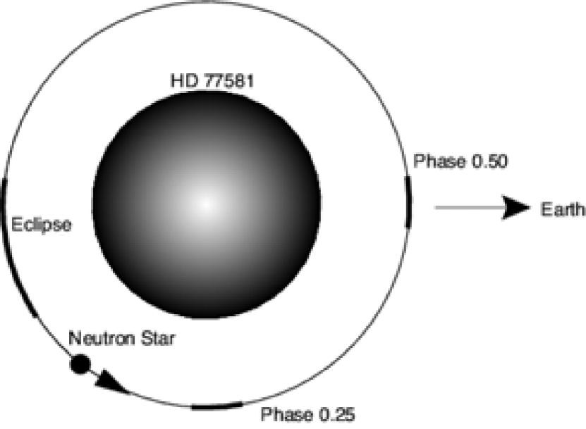
Figure 1.— The orbit of the neutron star in the Vela X-1 system. The observer is located along the horizontal axis on the right. The bold lines span the range of orbital phases covered by the Chandra observations.

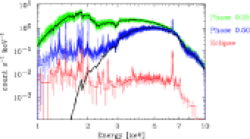
Figure 2.— The observed HEG spectra of Vela X-1. The green, blue, and red histograms show the spectra at phase 0.25, phase 0.50 and eclipse, respectively. The solid black lines represent best-fit continuum spectral models for phases 0.25 and 0.50 with parameters listed in Table 2.

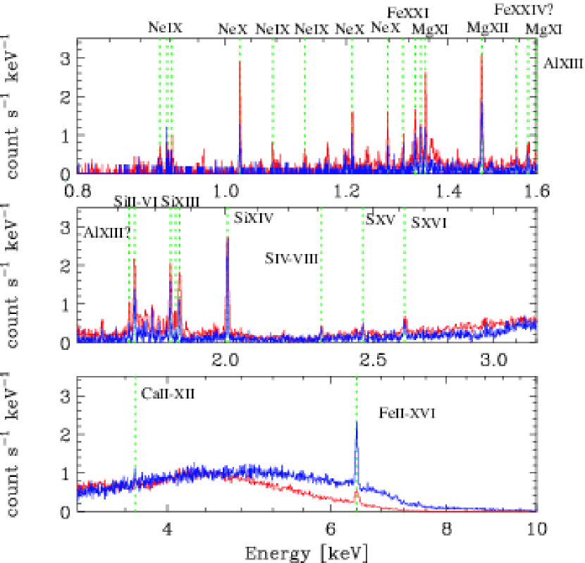
Figure 3.— A detailed view of the Vela X-1 spectrum at phase 0.50 – MEG data in red and HEG data in blue. The spectrum is dominated by discrete features below $E\sim 3~{}\rm{keV}$. The vertical green lines label the observed emission lines that are listed in Table 3.

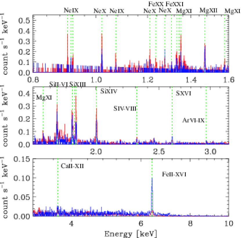
Figure 4.— Same as in Figure 3 for the eclipse phase. Note the striking similarity of the global emission line spectrum compared to that seen at phase 0.50. The vertical green lines label the emission lines listed in Table 4.

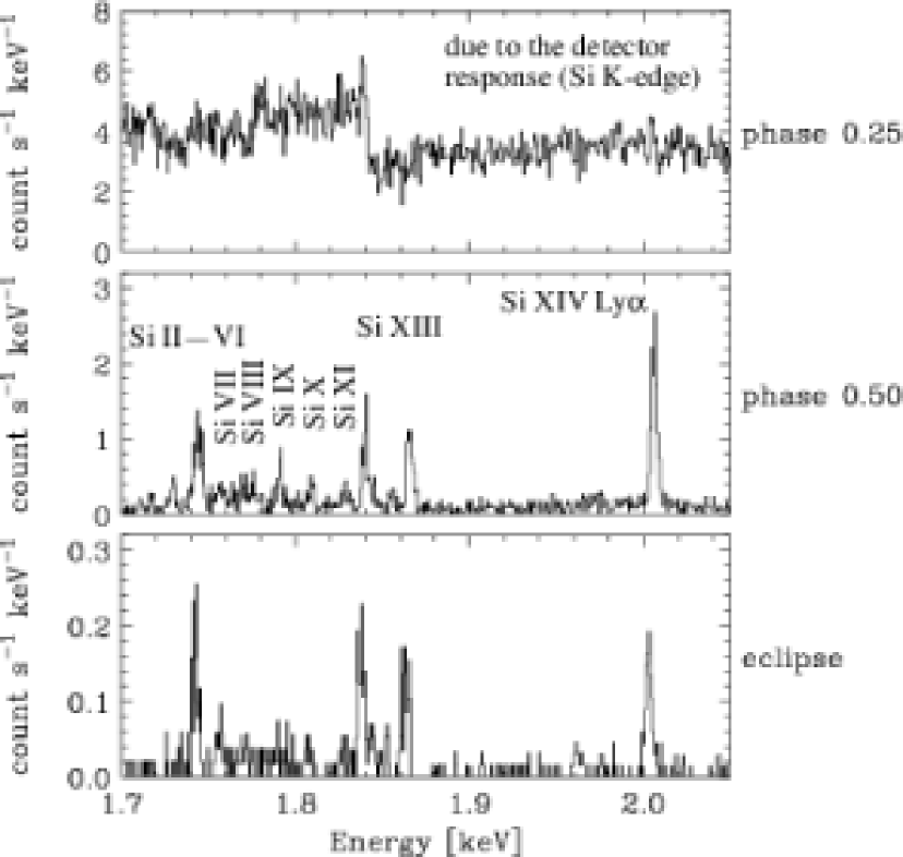
Figure 5.— The spectra of the Si K line complex observed at each orbital phase – phase 0.25 (top), phase 0.50 (middle), eclipse (bottom). The phase 0.25 spectrum is dominated by the intense continuum with possible evidence for weak absorption lines. The sharp drop at $E=1.84~{}\rm{keV}$ is due Si K photoelectric absorption in the detector. At phases 0.50 and eclipse, emission lines from a wide range of charge states are seen.

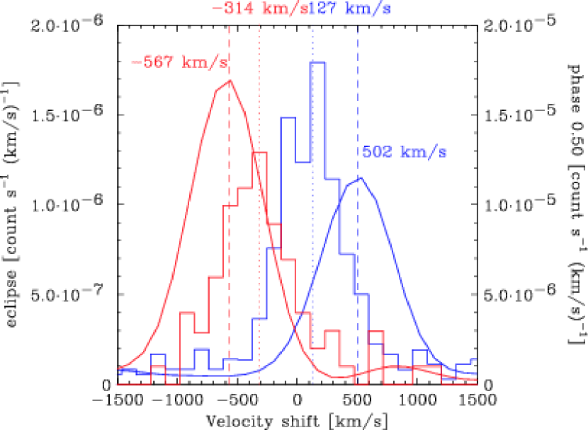
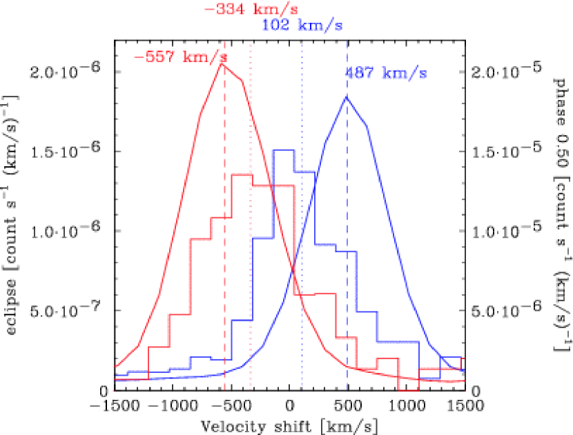
Figure 6.— Line profiles of Si XIV Ly$\alpha$ in the HEG spectrum (left) and Mg XII Ly$\alpha$ in the MEG spectrum (right) plotted at a function of the velocity. The blue and red histograms show the observed data at phase 0.50 and eclipse, respectively, and the smooth curves were made from the output of the Monte Carlo simulation (see § 4.6) convolved with the respective HEG/MEG response functions. Note the discrepancy between the data and model on the order of $200-400~{}\rm{km~{}s}^{-1}$ in the sense that the model predicts larger velocity amplitudes than the observed values.

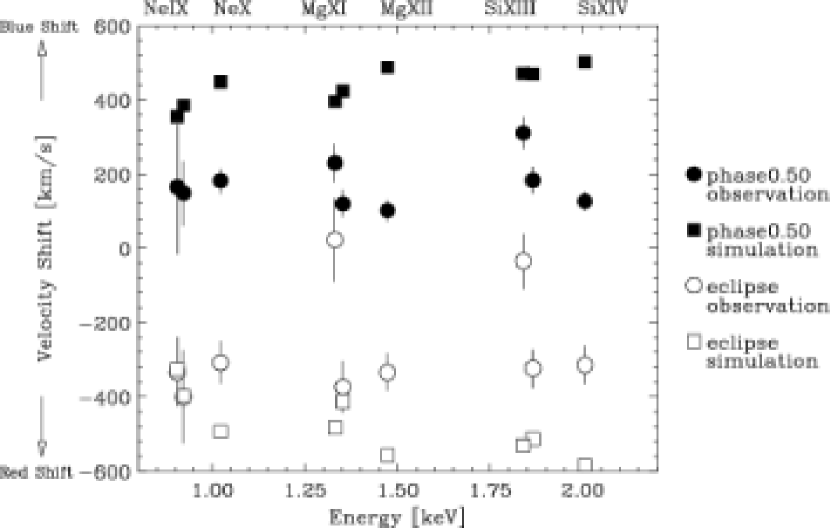
Figure 7.— The plot of the velocity shifts for emission lines from highly ionized ions. The circles represent values derived from the observations, and the squares are values derived from the Monte Carlo simulations (see § 4.6). Filled and open symbols are used to designate values derived from phase 0.50 and eclipse, respectively. As shown in Figure 6 for two particular lines, the lines from the other ions also systematically show a smaller velocity amplitude compared to the simulations.

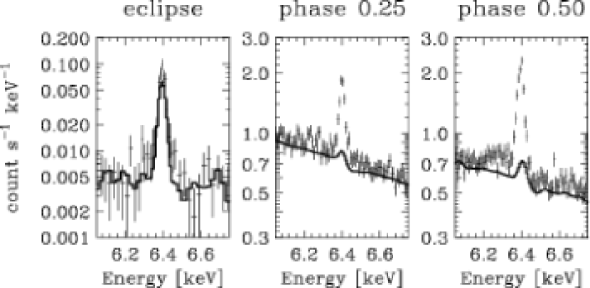
Figure 8.— The blown-up spectra of the iron K$\alpha$ region at the three orbital phases. The data points represent the HEG spectrum and the dark histograms show the Monte Carlo models, which include iron fluorescent X-rays from the stellar wind alone (see § 4.5). The model accounts for essentially all of the line flux observed during eclipse, but fails to reproduce the non-eclipse data by a large factor.

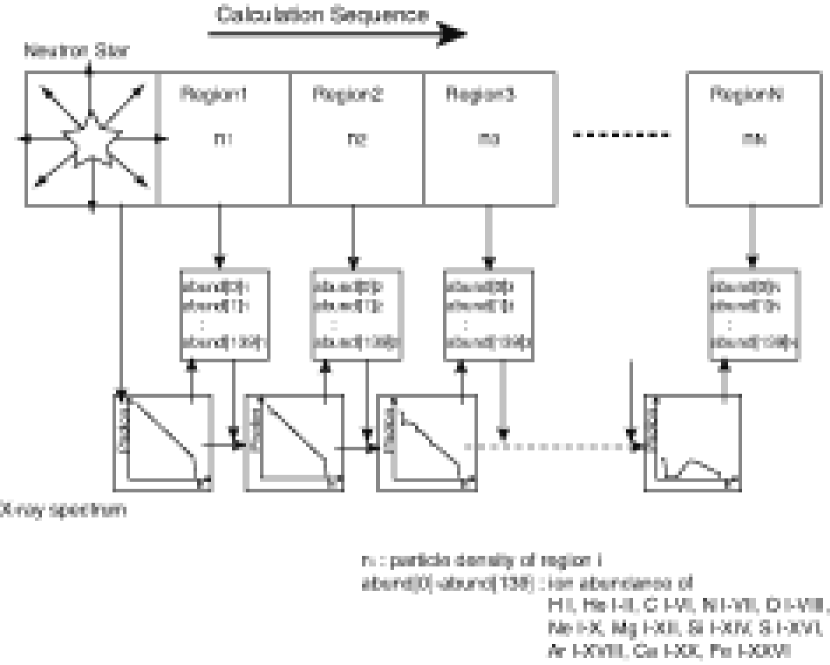
Figure 9.— A schematic diagram showing the sequence of how the ionization structure is calculated in the Monte Carlo simulator. The continuum photons from the neutron star (left) is propagated through each spatial cell and transfered to the next cell accounting for absorption.

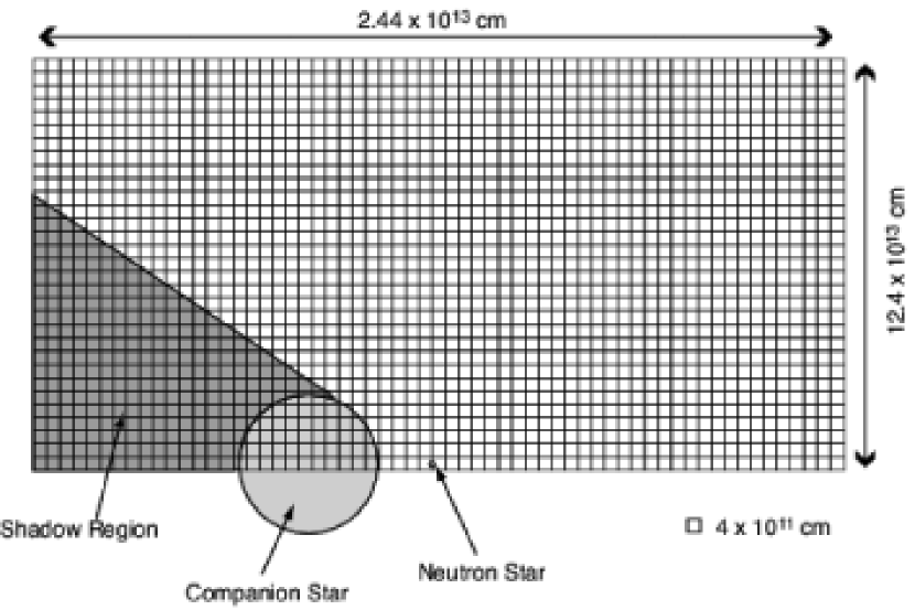
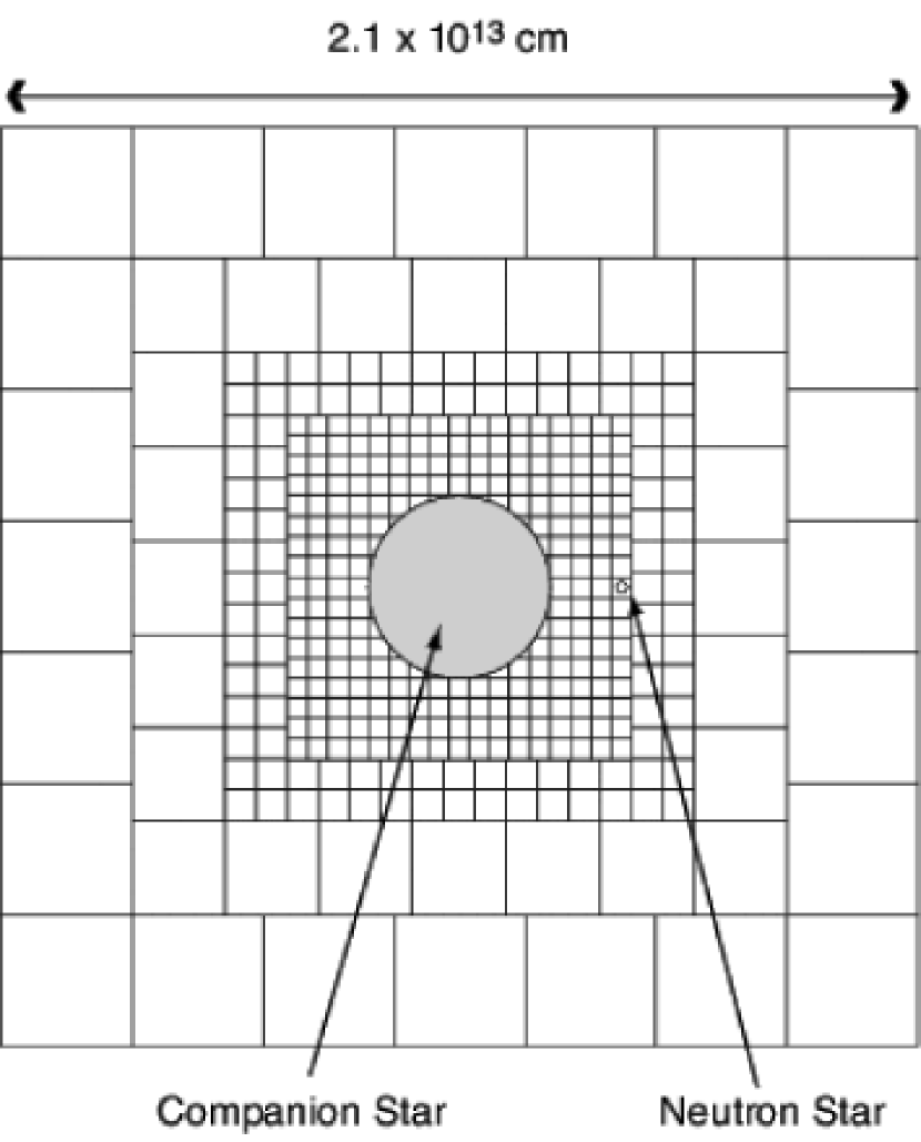
Figure 10.— The Vela X-1 geometry and spatial grids used in the calculation of the ionization structure (left) and the Monte Carlo spectral simulation (right).

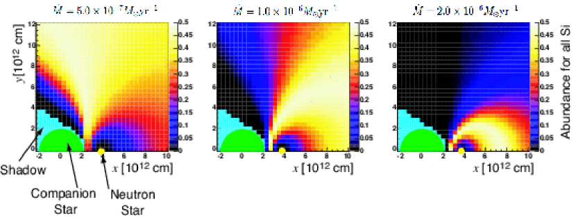
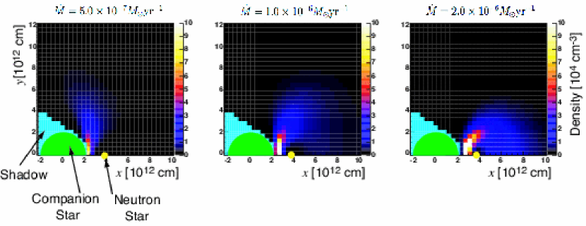
Figure 11.— The map of the H-like ion fraction of Si.

Figure 12.— The density map of H-like Si.

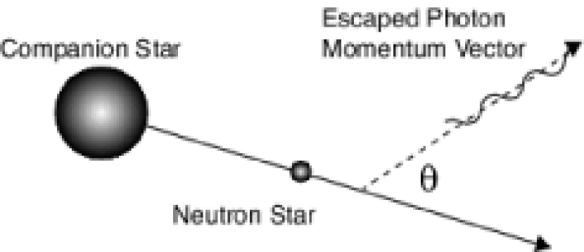
Figure 13.— The definition of the angle $\theta$, the angle of the outgoing photon relative to the line of centers.

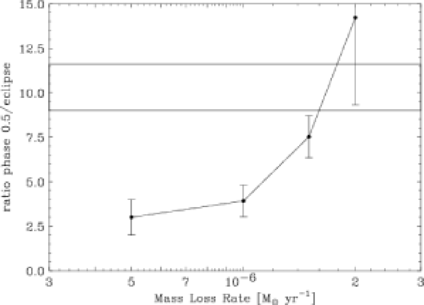
Figure 14.— Intensity ratio of Si Ly$\alpha$ between phase 0.5 and eclipse as a function of the mass-loss rate. Each point represents results derived from the Monte Carlo simulations, and the error bars corresponds to 1$\sigma$ Poisson error due to the limited number of trials. The two horizontal lines denote the 1$\sigma$ range of the observed value. This figure shows that the mass-loss rate in the Vela X-1 system is $\sim 1.5-2.0\times 10^{-6}~{}M_{\odot}~{}\rm{yr}^{-1}$.

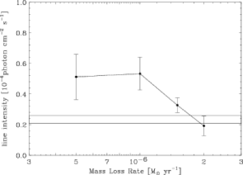
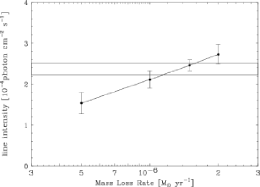
Figure 15.— The Si Ly$\alpha$ line intensity during eclipse (left) and for phase 0.50 (right) as a function of the mass-loss rate. The horizontal lines denote the 1$\sigma$ ranges of the observed values. As in Figure 14, a consistent solution can be obtained for a mass-loss rate of $\sim 1.5-2.0\times 10^{-6}~{}M_{\odot}~{}\rm{yr}^{-1}$.

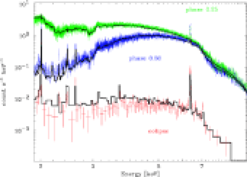
Figure 16.— Comparison of the simulated spectra with the observed data above 2 keV. The normalization of the simulation models are fixed between the three phases ranges, assuming that the average X-ray luminosity does not change. The simulated models are multiplied by a Galactic column density of $N_{\mathrm{H}}$ = 6 $\times$ $10^{21}$ cm^-2 and convolved with the instrument response.

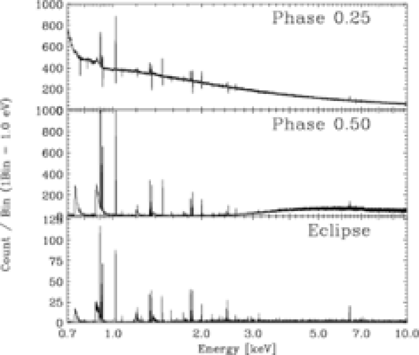
Figure 17.— Monte Carlo simulation spectra at the three phases for the mass loss rate of 1.5 $\times$ 10^-6 $M_{\sun}$ yr^-1. These spectra are not convolved with the instrumental response.

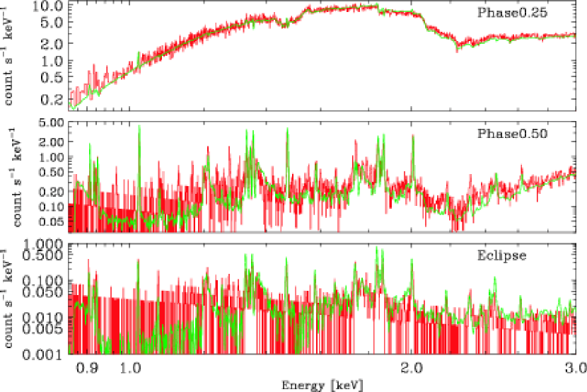
Figure 18.— Emission line spectra obtained with Chandra MEG. The red curves represent the data and the green lines show the Monte Carlo data convolved with MEG instrument response.

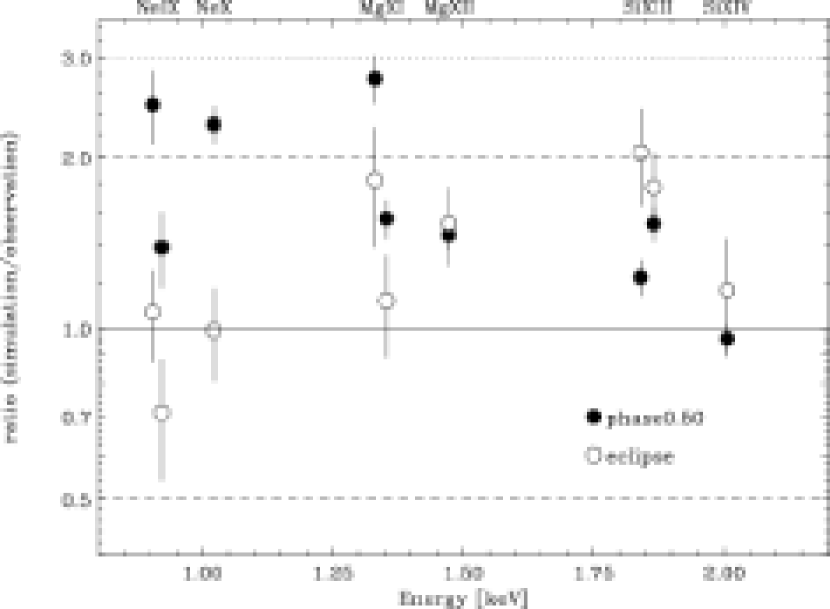
Figure 19.— The plots of the intensity ratios of the simulated lines and the observed lines. The filled and open circles show the results from phase 0.50 and eclipse, respectively. Each of the measured lines intensities are within a factor of 3 from the predicted values.

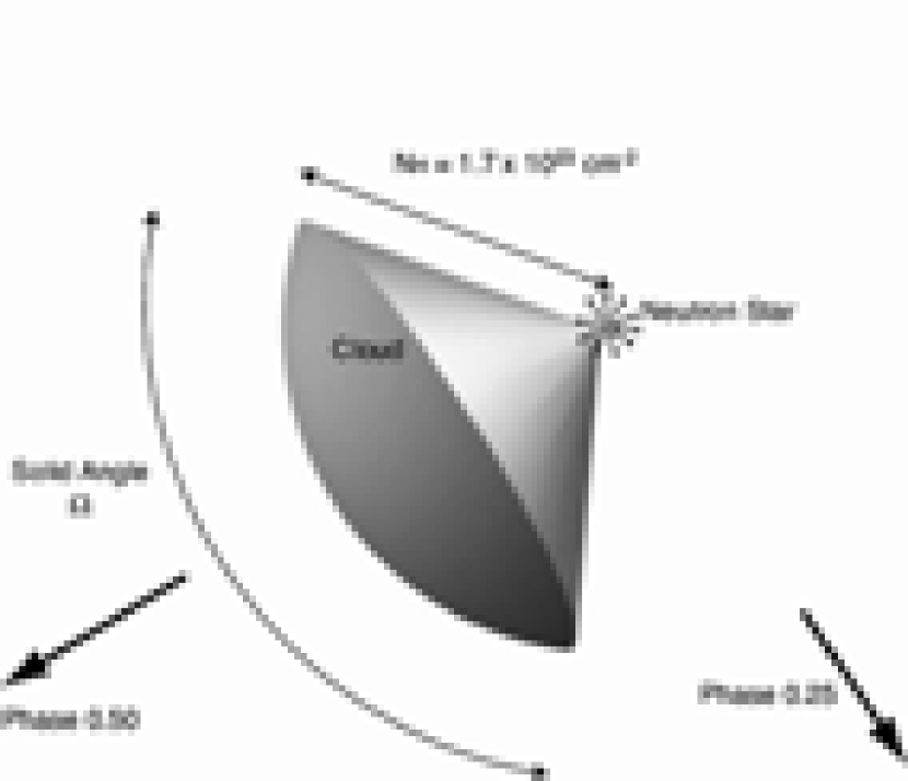
Figure 20.— Geometry of the cold cloud used in the Monte Carlo simulation to calculate the iron K$\alpha$ equivalent width.

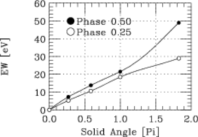
Figure 21.— Relation between the cloud’s solid angle and the equivalent width of the iron K$\alpha$ line calculated with a Monte Carlo simulation. The thickness of the cloud is $N_{\mathrm{H}}=1.7\times 10^{23}$ cm^-2 and assumed to be at a uniform density. Open and filled circles show the predicted equivalent width as observed at phases 0.25 and 0.50, respectively.

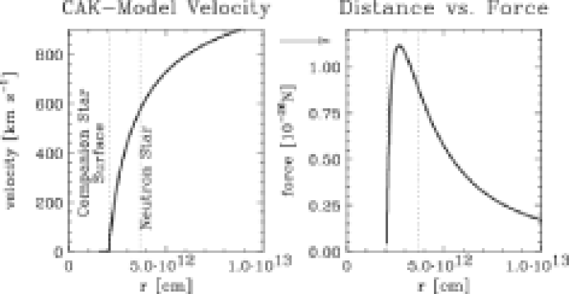
Figure 22.— The velocity profile of the CAK-model stellar wind with $v_{\infty}=1100$ km s^-1 and $\beta=0.8$ (left) and the force profile (right). The vertical dotted lines designate the location of the stellar surface and the neutron star. The force is numerically derived from the CAK-model velocity structure. Note that the force is most dominant in the region between the neutron star and the companion stellar surface.

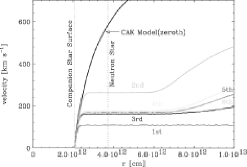
Figure 23.— The results of a 1-D calculation of the stellar wind velocity along the axis between the companion star and the neutron star accounting for X-ray photoionization as described in § 4.6.3. The mass loss rate is assumed to be $1.5\times 10^{-6}M_{\sun}\mathrm{yr}^{-1}$. The flattening of the velocity profile is due to X-ray photoionization destroying the ions that are capable of absorbing in the UV.

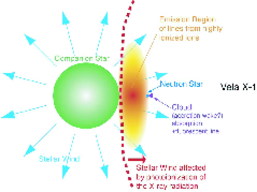
Figure 24.— A conceptual picture of the Vela X-1 system obtained from the present analysis.

References

- Band et al. (1990) Band, I.M., Trzhaskovskaya, M.B., Verner, D.A., & Yakovlev, D.G. 1990, A&A, 237, 267
- Barziv et al. (2001) Barziv, O., Kaper, L., van Kerkwijk, M.H., Telting, J.H., & van Paradijs, J. 2001, A&A, 377, 925
- Blondin et al. (1990) Blondin, J.M., Kallman, T.R., Fryxell, B.A., & Taam, R.E. 1990, ApJ, 356, 591
- Blondin, Stevens & Kallman (1991) Blondin, J.M., Stevens, I.R, & Kallman, T.R. 1991, ApJ, 371, 684
- Blondin (1994) Blondin, J.M. 1994, ApJ, 435, 756
- Bord et al. (1976) Bord, D.J., Mook, D.E., Petro, L., & Hiltner, W.A. 1976, ApJ, 203, 689
- Boroson et al. (2003) Boroson, B., Vrtilek, S.D., Kallman, T. & Corcoran, M., 2003, ApJ, 592, 516
- Brucato & Kristian (1972) Brucato, R.J., & Kristian, J. 1972, ApJ, 173, 105
- Castor, Abbott & Klein (1975) Castor, J.I., Abbott, D.C., & Klein, R.I. 1975, ApJ, 195, 157
- Dupree et al. (1980) Dupree, A.K. et al. 1980, ApJ, 238, 969
- Feldman (1992) Feldman, U. 1992, Physica Scripta. 46, 202
- Forman et al. (1973) Forman, W., Jones, C., Tananbaum, H., Gursky, H., Kellogg, E., & Giacconi, R. 1973, ApJ, 182, 103
- Goldstein et al. (2004) Goldstein, G., Huenemoerder, D.P. & Blank, D. 2004, AJ, 127, 2310
- Hiltner, Werner & Osmer (1972) Hiltner, W.A., Werner, J., & Osmer, P. 1972, ApJ, 175, L19
- Hutchings (1976) Hutchings, J.B. 1976, ApJ, 203, 438
- Inoue (1985) Inoue, H. 1985, Space Sci. Rev., 40, 317
- Kallman & White (1982) Kallman, T.R., & White, N.E. 1982, ApJ, 261, 35
- Kaper et al. (1993) Kaper, L., Hammerschlag-Hensberge, G., &van Loon, J.Th. 1993, A&A, 279, 485
- Krause (1979) Krause, M.O. 1979, J. Phys. Chem. Ref. Data, 8, 307
- Kreykenbohm et al. (1999) Kreykenbohm, I., Kretschmar, P., Wilms, J., Staubert, R., Kendziorra, E., Gruber, D.E., Heindl, W.A., & Rothschild, R.E. 1999, A&A, 341, 141
- Larkins (1977) Larkins, F.B. 1977, At. Data and Nucl. Data Tables, 20, 313
- MacGregor & Vitello (1982) MacGregor, K.B., & Vitello, P.A.J. 1982, ApJ, 259, 267
- Makishima et al. (1999) Makishima, K., Mihara, T., Nagase, F., & Tanaka, Y. 1999, ApJ, 525, 978
- Masai (1984) Masai, K. 1984, Ap&SS, 106, 391
- McClintock et al. (1976) McClintock, J.E. et al. 1976, ApJ, 206, 99
- Paerels et al. (2000) Paerels, F., Cottam, J., Sako, M., Liedahl, D.A., Brinkman, A.C., Van der Meer, R.L.J., Kaastra, J.S., & Predehl, P. 2000, ApJ, 533, L135
- Pauldrach, Puls & Kudritzki (1986) Pauldrach, A., Puls, J., & Kudritzki, R.P. 1986 A&A, 164, 86
- Prinja et al. (1990) Prinja, R.K., Barlow, M.J., & Howarth, I.D. 1990, ApJ, 361, 607
- Sadakane et al. (1985) Sadakane, K., Hirata, R., Jugaku, J., Kondo, Y., Matsuoka, M., Tanaka, Y., & Hammerschlag-Hensberge, G. 1985, ApJ, 288, 284
- Sako et al. (1999) Sako, M., Liedahl, D.A., Kahn, S.M., & Paerels, F. 1999, ApJ, 525, 921
- Salem, Panossian & Krause (1974) Salem, S.I., Panossian, S.L., & Krause, R.A. 1974, At. Data and Nucl. Data Tables, 14, 91
- Sato et al. (1986) Sato, N., Hayakawa, S., Nagase, F., Masai, K., Dotani, T., Inoue, H., Makino, F., Makishima, K., & Ohashi, T. 1986, PASJ, 38, 731
- Sawada, Matsuda & Hachisu (1986) Sawada, K., Matsuda, T. & Hachisu, I. 1986, MNRAS, 221, 679
- Schulz et al. (2002) Schulz, N.S., Canizares, C.R., Lee, J.C., & Sako, M. 2002, ApJ, 564, L21
- van Kerkwijk et al. (1995) van Kerkwijk, M.H., van Paradijs, J., Hammerschlag-Hensberge, G., Kaper, L., & Sterken, C. 1995, A&A, 303, 483
- van Paradijs et al. (1977) van Pradijs, J., Zuiderwijk, E.J., Takens, R.J., & Hammerschlag-Hensberge, G. 1977, A&AS, 30, 195
- Watanabe et al. (2003) Watanabe, S., et al. 2003, ApJ, 597, L37