Global MHD simulations of stratified and turbulent protoplanetary discs. I. Model properties

Abstract

Aims. We present the results of global 3-D MHD simulations of stratified and turbulent protoplanetary disc models. The aim of this work is to develop thin disc models capable of sustaining turbulence for long run times, which can be used for on–going studies of planet formation in turbulent discs.

Methods. The results are obtained using two codes written in spherical coordinates: GLOBAL and NIRVANA. Both are time–explicit and use finite differences along with the Constrained Transport algorithm to evolve the equations of MHD.

Results. In the presence of a weak toroidal magnetic field, a thin protoplanetary disc in hydrostatic equilibrium is destabilised by the magnetorotational instability (MRI). When the resolution is large enough ($\sim 25$ vertical grid cells per scale height), the entire disc settles into a turbulent quasi steady–state after about $300$ orbits. Angular momentum is transported outward such that the standard $\alpha$ parameter is roughly $4-6\times 10^{-3}$. We find that the initial toroidal flux is expelled from the disc midplane and that the disc behaves essentially as a quasi–zero net flux disc for the remainder of the simulation. As in previous studies, the disc develops a dual structure composed of an MRI–driven turbulent core around its midplane, and a magnetised corona stable to the MRI near its surface. By varying disc parameters and boundary conditions, we show that these basic properties of the models are robust.

Conclusions. The high resolution disc models we present in this paper achieve a quasi–steady state and sustain turbulence for hundreds of orbits. As such, they are ideally suited to the study of outstanding problems in planet formation such as disc–planet interactions and dust dynamics.

1 Introduction

Observational surveys of star forming regions in the Galaxy have revealed the ubiquity of rotationally supported discs of gas and dust orbiting young stars (e.g. Beckwith & Sargent 1996; O’dell et al. 1993; Stauffer et al. 1994; Sicilia-Aguilar et al. 2006; Kessler-Silacci et al. 2006). It is commonly believed that these discs are the likely sites of planetary formation (Safronov 1969; Lissauer 1993). The discovery of numerous extrasolar planets has increased the need for greater understanding of their properties so that accurate models of planet formation can be developed.

These “protoplanetary” discs often show evidence for active accretion with a canonical mass flow rate onto the central star of $\sim 10^{-8}$ M_⊙ yr^-1 (e.g. Sicilia-Aguilar et al. 2004), requiring a source of anomalous viscosity to transport angular momentum outward. It has long been believed that this is provided by turbulence within the disc (e.g. Shakura & Sunyaev 1973). So far only one mechanism has been shown to work reliably: MHD turbulence generated by the magnetorotational instability (MRI) (Balbus & Hawley 1991; Hawley & Balbus 1991). Given the cool and dense nature of protoplanetary discs, there are questions about the global applicability of the MRI in such environments as the ionisation fraction is low (Blaes & Balbus 1994). Models suggest that protoplanetary discs are likely to have both magnetically active zones, where the disc is turbulent, and adjacent magnetically ‘dead-zones’ where the flow is laminar (e.g. Gammie 1996; Fromang et al. 2002; Ilgner & Nelson 2006). In this paper we focus on ideal MHD simulations of protoplanetary discs. We will examine the dynamics of ‘dead–zones’ in future work.

Non linear numerical simulations performed using the local shearing box formalism (e.g. Hawley & Balbus 1991; Hawley et al. 1996; Brandenburg et al. 1996) have shown that the saturated non linear outcome of the MRI is MHD turbulence having an effective viscous stress parameter $\alpha$ between $\sim 5\times 10^{-3}$ and $\sim 0.1$, depending on the magnetic field configuration. Outward angular momentum transport can thus occur at the rate required to match observed accretion signatures onto T Tauri stars (see, for example, Hartmann et al. 1998, who quote $\alpha\sim 0.01$ as being suggested by the observations). Much of this early simulation work was performed in discs with no vertical stratification, and so was useful in determining the nonlinear outcome of the MRI, but did not provide insights into the global structure of these discs in either the radial or vertical direction. The question of their vertical structure was addressed by Stone et al. (1996) and Miller & Stone (2000) who performed shearing box simulations of vertically stratified discs. A basic result to come out of these studies is that the discs evolve to a structure consisting of a dense region around the miplane where turbulence is driven by the MRI, sandwiched between a tenuous and magnetically dominated corona which is highly dynamic, but stable against the MRI.

Global MHD simulations of turbulent discs (e.g. Armitage 1998; Hawley 2000, 2001; Steinacker & Papaloizou 2002; Papaloizou & Nelson 2003) confirm the basic picture provided by the local shearing box simulations. These early global simulations considered the radial structure of turbulent disc models, but employed non stratified cylindrical disc models. Recent work has been performed examining the dynamics of global, vertically stratified turbulent disc models, and has focussed on thick accretion tori around black holes, using either the Paczynski–Witta potential (Hawley 2000; Hawley & Krolik 2001; Hawley et al. 2001) or simulating accretion flows in the full Kerr metric (e.g. De Villiers et al. 2003). The starting conditions for these models are usually thick, constant angular momentum tori for which the gas is assumed to be non–radiating. These quickly evolve into thick accretion discs for which $H/R>0.1$. To date, there have been no published simulations of vertically stratified thin discs undergoing MHD turbulence (i.e. discs more akin to protoplanetary discs). In part this is because of the increased computational burden associated with simulating thin discs due to the higher resolution requirements.

The aim of this paper is to present and analyse a suite of MHD simulations of global, stratified, turbulent, protoplanetary disc models with $H/R\leq 0.1$. We focus on the global structure of the discs, and analyse how modifications to the boundary conditions and disc thickness affect the results. The longer term goal is to use these models to examine a range of problems in planetary formation in the context of turbulent, vertically stratified discs. As such this paper is the first in a series. Future publications will address problems such as: the evolution of dust in turbulent discs; the orbital evolution of planetesimals and low mass planets; gap formation and gas accretion by giant protoplanets; the dynamical evolution of dead–zones. A number of previous studies have addressed these issues using cylindrical models: Nelson & Papaloizou (2003); Papaloizou et al. (2004); Nelson & Papaloizou (2004); Nelson (2005) studied gap formation and planet formation in turbulent discs. They showed in particular that type I migration becomes stochastic because of the turbulent density fluctuations in the disc. Fromang & Nelson (2005) also used cylindrical models to study the radial migration of solid bodies due to gas drag. They found rapid accumulation of meter size bodies in anticyclonic vortices apparently resulting from the turbulence. Another key problem in planet formation, dust settling in turbulent discs, has been studied recently using shearing box models (Johansen et al. 2006; Fromang & Papaloizou 2006; Turner et al. 2006). Because of the local approach, these analyses had to ignore radial drift. All of these issues are likely to be affected by the simultaneous treatment of radial and vertical stratification that we consider in this present work.

The plan of the paper is as follows: in section 2, we present the basic equations, notations, and diagnostics we use in this work. The set-up of our simulations is detailed in section 3 and we present their results in section 4. We focus in particular on their global structure, and sensitivity to numerical issues such as resolution and boundary conditions. Finally, in section 5, we summarise our results and highlight future improvements that will be added to the models.

2 Basic equations

The equations we seek to solve are the standard equations of MHD in a frame rotating with the angular velocity $\Omega_{rot}$. In Gaussian units these may be expressed as:

$$\frac{\partial\rho}{\partial t}+\mbox{\boldmath{$\nabla$}}\mbox{\boldmath{$\cdot$}}(\rho\mbox{\boldmath{$v$}})=0\,,$$ (1)

$$\frac{\partial\mbox{\boldmath{$v$}}}{\partial t}+(\mbox{\boldmath{$v$}}\mbox{\boldmath{$\cdot$}}\mbox{\boldmath{$\nabla$}})\mbox{\boldmath{$v$}}+2\mbox{\boldmath{$\Omega_{rot}$}}\mbox{\boldmath{$\times$}}\mbox{\boldmath{$v$}}=-\frac{1}{\rho}\mbox{\boldmath{$\nabla$}}P-\nabla\Phi+\frac{1}{4\pi\rho}(\mbox{\boldmath{$\nabla$}}\mbox{\boldmath{$\times$}}\mbox{\boldmath{$B$}})\mbox{\boldmath{$\times$}}\mbox{\boldmath{$B$}}\,,$$ (2)

$$\frac{\partial\mbox{\boldmath{$B$}}}{\partial t}=\mbox{\boldmath{$\nabla$}}\mbox{\boldmath{$\times$}}(\mbox{\boldmath{$v$}}\mbox{\boldmath{$\times$}}\mbox{\boldmath{$B$}}-\eta\nabla\mbox{\boldmath{$\times$}}\mbox{\boldmath{$B$}})\,.$$ (3)

The symbols have their usual meanings: $\rho$ is the density, $v$ is the velocity, $P$ is the gas pressure, $B$ is the magnetic field, $\eta$ is the magnetic diffusivity, and $\Phi$ is the sum of the gravitational and centrifugal potentials. In the following discussion we will use two systems of coordinates: cylindrical coordinates $(R,\phi,Z)$ and spherical coordinates $(r,\theta,\phi)$. Using the later, $\Phi$ becomes

$$\Phi=-\frac{1}{2}\Omega_{rot}^{2}r^{2}\sin^{2}\theta-\frac{GM}{r}$$ (4)

where $G$ is the gravitational constant and $M$ the mass of the central protostar. To complete equations (1)–(3), we use a locally isothermal equation of state:

$$P=c(R)^{2}\rho$$ (5)

where $c(R)$ is the sound speed which is a fixed function of position.

2.1 Averaged quantities and connection to viscous disc theory

When presenting the results of our calculations we make use of a number of averaged quantities. For a quantity $Q$, we define the average ${\overline{Q}(R,t)}$ through

$${\overline{Q}}(R,t)=\frac{\frac{1}{\Delta\phi}\int\int\rho Q(R,\phi,Z,t)dzd\phi}{\frac{1}{\Delta\phi}\int\int\rho dzd\phi}$$ (6)

where $\Delta\phi=\phi_{max}-\phi_{min}$ is the size of the azimuthal domain (which is less than $2\pi$ in the disc models we present later in this paper). The integrals are taken over the total disc height and azimuth. We define the disc surface density through

$$\Sigma(R)={\frac{1}{\Delta\phi}\int\int\rho dzd\phi}$$ (7)

Note that without loss of generality we can also include a time–average within our averaging procedure. In this case the quantity ${\overline{Q}}(R,t)$ becomes:

$${\overline{Q}}(R,t)=\frac{1}{2\Delta t}\int_{t-\Delta t}^{t+\Delta t}{\overline{Q}}(R,t)dt$$ (8)

where $2\Delta t$ is the time interval over which the averaging procedure is performed.

We now consider the connection between the turbulent disc models and standard viscous disc theory (e.g. Shakura & Sunyaev 1973; Balbus & Papaloizou 1999; Papaloizou & Nelson 2003). Averaging the continuity equation (1) gives

$$\frac{\partial\Sigma}{\partial t}+\frac{1}{R}\frac{\partial}{\partial R}\left(R\Sigma{\overline{v}_{R}}\right)=0.$$ (9)

Consider the azimuthal component of the momentum equation (2). Multiplying by $R$ to give an equation for the conservation of angular momentum about the $Z$ axis, and averaging over the disc height and azimuth gives:

$$\frac{\partial}{\partial t}\left(\Sigma{\overline{j}}\right)+\frac{1}{R}\frac{\partial}{\partial R}\left(R\Sigma{\overline{j}}\,{\overline{v}_{R}}\right)= - \frac{1}{R}\frac{\partial}{\partial R}\left(R^{2}\Sigma\overline{\delta v_{\phi}\delta v_{R}}\right)$$ (10)

$$+ \frac{1}{R}\frac{\partial}{\partial R}\left[R^{2}\Sigma\overline{\left(\frac{B_{\phi}B_{R}}{4\pi\rho}\right)}\right].$$

Here $j$ is the specific angular momentum, $Rv_{\phi}$, and we have used the relations $v_{R}={\overline{v}_{R}}+\delta v_{R}$ and $v_{\phi}={\overline{v}_{\phi}}+\delta v_{\phi}$, where $\delta v_{R}$ and $\delta v_{\phi}$ are the fluctuations in the radial and azimuthal velocities. Note that we have neglected terms due to the pressure gradient in equation (10) as the transport of angular momentum within the disc is primarily due to Reynolds and Maxwell stresses. These are given by the two terms on the right hand side of equation (10), and we define the Reynolds stress by

$${\overline{T}_{R}}=\Sigma\overline{\delta v_{\phi}\delta v_{R}}$$ (11)

and the Maxwell stress by

$${\overline{T}_{M}}=\Sigma\overline{\left(\frac{B_{\phi}B_{R}}{4\pi\rho}\right)}.$$ (12)

We define the viscous stress parameter $\alpha$ through

$$\alpha=\frac{{\overline{T}_{R}}-{\overline{T}_{M}}}{{\overline{P}}}$$ (13)

where ${\overline{P}}$ is the averaged gas pressure. In the discussion of our simulation results presented later in this paper we refer to $\alpha_{M}$ and $\alpha_{R}$, which are the Maxwell and Reynolds stress contributions to the total $\alpha$ value defined in equation (13). We also discuss the volume averages of $\alpha$, $\alpha_{M}$ and $\alpha_{R}$ which we denote as $\langle\alpha\rangle$, $\langle\alpha_{M}\rangle$ and $\langle\alpha_{R}\rangle$.

Combining equations (9) and (10) gives:

$$\Sigma\frac{\partial{\overline{j}}}{\partial t}+\Sigma{\overline{v}_{R}}\frac{\partial{\overline{j}}}{\partial R}=-\frac{1}{R}\frac{\partial}{\partial R}\left(R^{2}{\overline{T}_{R}}-R^{2}{\overline{T}_{M}}\right)$$ (14)

Assuming that the averaged specific angular momentum ${\overline{j}}(R)$ is time independent, we obtain an equation for the averaged radial velocity that is the equivalent of a similar expression obtained in standard viscous thin disc theory:

$${\overline{v}_{R}}=-\frac{1}{R\Sigma}\left(\frac{\partial{\overline{j}}}{\partial R}\right)^{-1}\frac{\partial}{\partial R}\left(R^{2}{\overline{T}_{R}}-R^{2}{\overline{T}_{M}}\right).$$ (15)

By obtaining time averaged values of ${\overline{T}_{R}}(R)$, ${\overline{T}_{M}}(R)$, ${\overline{j}}(R)$, ${\overline{v}_{R}}(R)$ and $\Sigma(R)$ from our numerical simulations, we are able to compare the value of ${\overline{v}_{R}}(R)$ obtained directly in the simulations to that predicted by equation (15). Hence we can examine how well our 3–D turbulent and stratified protoplanetary disc models are described by thin disc theory, subject to an appropriate time average. When calculating these averages in the simulations, which are performed using spherical polar coordinates, we perform the vertical integration by replacing $dz\rightarrow r\sin{\theta}d\theta$, and integrate along the meridian at fixed $r$ and $\phi$.

Model	$c_{0}$	Resolution	Azimutal extent	Vertical extent	Inner radial BC	Outer radial BC	Vertical BC	Code
S1a	0.07	$(272,90,126)$	$\pi/4$	0.3	Reflecting	Reflecting	Outflow	GLOBAL
S1b	0.07	$(272,90,126)$	$\pi/4$	0.3	Reflecting	Reflecting	Outflow	NIRAVANA
S2	0.07	$(455,150,213)$	$\pi/4$	0.3	Reflecting	Reflecting	Outflow	GLOBAL
S3	0.07	$(455,150,285)$	$\pi/4$	0.4	Reflecting	Reflecting	Outflow	GLOBAL
S4	0.07	$(456,150,210)$	$\pi/4$	0.3	Reflecting	Reflecting	Periodic	NIRVANA
S5	0.1	$(360,120,210)$	$\pi/4$	0.43	Outflow	Reflecting	Outflow	NIRVANA
C1	0.07	$(455,150,40)$	$\pi/4$	0.42	Reflecting	Reflecting	Periodic	GLOBAL
C2	0.07	$(260,152,44)$	$\pi/2$	0.28	Reflecting	Reflecting	Periodic	GLOBAL

Table 1: Properties of the models described in this paper. The first column gives the model label, the second gives the sound speed at $r=r_{0}$. The third, fourth and fifth columns describe the resolution and the extent of the numerical box. The type of boundary conditions we used are given in columns 6 ,7 and 8, while the last column indicates the code used to run that particular model. For the detailed set–up of model C2, see section 3.2 or Fromang & Nelson (2005).

3 Numerical Simulations

We used two codes to solve the MHD equations described in section 2: GLOBAL (Hawley & Stone 1995) and NIRVANA (Ziegler & Yorke 1997). GLOBAL, originally written in cylindrical geometry, was modified to operate using spherical coordinates. Both codes are time explicit, use finite-differences to calculate spatial derivatives and the Method of Characteristics Constrained Transport (MOCCT) algorithm to evolve the magnetic field. They have been widely tested in the past on a variety of different problems relating to turbulent protoplanetary discs, making them particularly well suited to undertake the computationally demanding problem of simulating stratified protoplanetary discs models.

3.1 Stratified disc model set-up

At time $t=0$ we specify a spatial distribution for the hydrodynamic variables that is as close as possible to a stratified thin disc in hydrostatic equilibrium. Except for the vertical stratification, the model properties are very close to those of Papaloizou & Nelson (2003). The mass density $\rho$ and angular velocity $\Omega$ are defined using:

$$\rho = \rho_{0}\left(\frac{R_{0}}{R}\right)^{3/2}exp\left(-\frac{Z^{2}}{2H^{2}}\right)\,,$$ (16)

$$\Omega = \sqrt{\frac{GM}{R^{3}}}.$$ (17)

The radial and meridional velocities $v_{r}$ and $v_{\theta}$ are given small random perturbations (using a uniform distribution with amplitude $2.5$ % of the sound speed). The disc semi-thickness $H$ is related to disc parameters through

$$H=\frac{c(R)}{\Omega}\,.$$ (18)

In the absence of magnetic fields, the initial disc model is completely determined once the function $c(R)$ is given. In the following, we used:

$$c(R)=c_{0}\left(\frac{R_{0}}{R}\right)^{1/2}$$ (19)

such that $H/R$ is constant in the models. Using these relations, the surface density $\Sigma$ satifies

$$\Sigma=\Sigma_{0}\left(\frac{R_{0}}{R}\right)^{1/2}$$ (20)

where $\Sigma_{0}=2\rho_{0}c_{0}R_{0}^{3/2}/\sqrt{GM}$.

The constants appearing in the above equations are given values $GM=1$, $R_{0}=1$, $\rho_{0}=1$ and $\Omega_{rot}=0.5$. Depending on the models, $c_{0}$ is either equal to $0.07$ or $0.1$ (see table 1). The computational domain extends from $R_{in}=1$ to $R_{out}=8$ in the radial direction. The vertical and azimuthal extent depend on the model. But in all of them, at least $8.5$ scale heights are covered in $\theta$ in order to provide a good description of both the disc midplane and corona. When discussing simulation results in this paper, time will be quoted in units of the orbital time at the inner edge of the computational domain. With our definitions, a time span of $500$ orbits at $r=R_{in}$ (which is the typical duration of a given model) corresponds to $177$ orbits at $r=2$, $63$ orbits at $r=4$ and $27$ orbits at $r=7$.

Before adding the magnetic field, the above model was run as a purely hydrodynamic disc. Using reflecting boundary conditions in $r$, periodic boundary conditions in $\phi$ and outflow boundary conditions in $\theta$, we found it to stay very close to the initial model description presented above. In particular, we found no sign of the transient growth of hydrodynamic perturbations recently proposed in the literature (Ioannou & Kakouris 2001; Afshordi et al. 2005; Mukhopadhyay et al. 2005). The kinetic energy then decays on a time scale of $\sim 10$ orbits (some wavelike motions are then excited by the imperfect nature of the boundary conditions on time scales of hundreds of orbits, but the associated kinetic energy always remains smaller than in the MHD case by at least an order of magnitude).

In the MHD runs, a toroidal magnetic field was added to the disc at $t=0$. It is defined to be nonzero in the region of the disc satisfying $2.5<r<6$ and $|\theta-\pi/2|<\theta_{out}^{mag}$. We took $\theta_{out}^{mag}=0.1$ in all of the models, except for model S5 for which $\theta_{out}^{mag}=0.2$. The strength of the field is such that the ratio $\beta$ of the thermal pressure to the magnetic pressure is everywhere equal to $\beta_{0}=25$. Previous global models of such configurations have proved to be unstable to the MRI and to generate MHD turbulence that spreads into the entire computational domain. We emphasize here that the flux of this magnetic field in the $\phi$ direction is nonzero at the beginning of the calculation.

3.1.1 Boundary conditions

We now come onto the boundary conditions. In principle it is possible to use reflecting or outflow boundary conditions at the inner and outer disc radii. Reflecting boundary conditions are unsuitable as waves excited by the turbulence then tend to rattle around the computational domain in an unphysical manner. Outflow conditions were tried in test calculations but proved to be unsuitable because of excessive mass loss out of the computational domain. Instead we added a non turbulent buffer zone close to each radial boundary (for all runs except S5, see below), the inner one extending from $r=R_{in}$ to $r=2$, the outer one extending from $r=7$ to $r=R_{out}$. In both buffer zones, we included a linear viscosity $q^{lin}$ with coefficient $C_{1}$ (see the definitions of Stone & Norman 1992), to damp fluid motion, and resistivity, $\eta$, to create a region that is stable to the MRI and therefore non turbulent near the boundary. Both dissipation coefficients increase linearly from the boundary of the buffer zones toward the boundary of the computational domain. In all cases except model S3, their maximum value at the inner boundary is $C_{1}=C_{1,in}=1$ and $\eta=\eta_{in}=4.9\times 10^{-4}$, while they reach $C_{1}=C_{1,out}=5$ and $\eta=\eta_{out}=10^{-3}$ at the outer boundary. In model S3, we used $C_{1,in}=1$, $C_{1,out}=30$, $\eta_{in}=2\times 10^{-4}$ and $\eta_{out}=10^{-2}$. Using this set-up, we found that the turbulent velocity fluctuations and magnetic stresses damp smoothly in the buffer zones.

For very long integration times, we found that mass tends to accumulate at the interface between the inner buffer zone and the active disc. This is expected for such a closed boundary condition. To try to solve this problem, we modified the inner boundary condition in model S5 and used a ‘viscous outflow condition’ (the outer radial boundary is kept unchanged). The viscous outflow condition specifies the radial outflow velocity in the inner radial boundary using the expression $v_{r}=-3/2\alpha c_{s}^{2}/\Omega$ there. A value of $\alpha=5\times 10^{-3}$ was adopted, in basic agreement with the transport coefficient resulting from the nonlinear evolution of the MRI (see below). The magnetic field boundary condition at the disc inner edge defines the field to be normal to the boundary with magnitude defined by the $\nabla.{\bf B}=0$ condition (e.g. Hawley 2000).

The boundary conditions in the $\theta$ direction are also of some importance in constructing stratified models. In local simulations using the shearing box approximation, Stone et al. (1996) reported very little effect of the boundary conditions. Nevertheless, we investigated their importance by running two types of boundary conditions: outflow and periodic. The latter is less physical but has the advantage of preserving the total flux of the magnetic field and the vanishing value of its divergence. The former was implemented in two different ways: in GLOBAL, a zero gradient boundary condition was applied on all the variables, including the magnetic field (Miller & Stone 2000). NIRVANA, on the other hand, forces the magnetic field to become normal to the boundary and still satisfy the condition $\mbox{\boldmath{$\nabla$}}\mbox{\boldmath{$\cdot$}}\mbox{\boldmath{$B$}}=0$ (Hawley 2000). The comparison between these different alternatives gives an insight to their importance on the global structure of the disc.

In the upper layers of the disc, strong magnetic fields tend to develop during the simulation. Because of the low density there, the associated Alfvén velocity becomes very large and the time step consequently very small. To prevent this from happening, we used the Alfvén speed limiter first introduced by Miller & Stone (2000) whose effect is to prevent the Alfvén speed becoming significantly larger than a user-defined threshold $v_{A}^{c}$. In the simulations presented in this paper, we used a uniform value of $v_{A}^{c}=0.7$.

3.2 Cylindrical models

In order to examine the effect of stratification, we ran a non stratified cylindrical model, labelled C1. The set–up was very similar to that for model S2. The vertical computational domain covered $-0.21\leq Z\leq 0.21$, and the initial magnetic field was a zero–net flux toroidal field defined by:

$$B_{\phi}=B_{0}\cos\left(6\pi\frac{R-R_{in}}{R_{out}-R_{in}}\right)\,.$$ (21)

$B_{0}$ is calculated such that the average value of $<\beta>=25$. We also consider another cylindrical disc run, C2, which used a net flux toroidal field with $\beta=270$ and was described in detail in Fromang & Nelson (2005). Because of the vertical periodic boundaries, the magnetic flux is conserved in these models.

3.3 Model descriptions

The detailed properties of the models we ran are described in table 1. Column $1$ gives their label. Column $2$ indicates the value of the parameter $c_{0}$. Given that $GM=1$ in our simulations, this is also equal to $H/R$. The resolution, the size of the computational box in the $\phi$ and $\theta$ directions are respectively given in columns $3$, $4$ and $5$. The type of boundary conditions we use at the inner and outer radial boundary and in the $\theta$ direction are shown by columns $6$, $7$ and 8. Finally, the code we use for each particular model is indicated by column $9$. Note that runs C1 and C2 are cylindrical disc models (see section 3.2).

4 Results

We now present the results of our simulations. Although differences in detail are found when comparing our various runs, a common picture of the early evolution of our models emerges. The magnetised regions of the initial discs become unstable to the MRI on the local dynamical time scale, in broad agreement with linear theory. Dynamo action associated with the MRI causes the local field to amplify, and as turbulence develops the field buoyantly rises from the regions near the midplane toward the disc surface. Initially the stresses associated with the field as it rises into these upper regions cause rapid transport of angular momentum there, allowing the magnetised fluid to spread rapidly through the disc in the radial direction near the disc surface. Contemporaneously the growth of the MRI throughout the magnetised core of the models causes the disc to become globally turbulent on a time scale of $\sim 100$ orbits. The end result is a disc whose global structure consists of a magnetically subdominant core within $\sim 2H$ of the disc midplane which remains highly turbulent due to continuing instability to the MRI, above and below which reside a magnetised and highly dynamic corona which becomes magnetically dominant near the disc surface and stable to the MRI. Angular momentum transport and associated mass flow through the disc allows magnetic field to diffuse into the resistive regions near the radial boundaries, where the fluid remains non turbulent because of the resistivity and viscosity there.

4.1 Dependance on resolution

Figure 1: Time history of $\langle\alpha_{M}\rangle$ obtained in model S1a (solid) and S1b (dashed line). The agreeement between the two curves shows that GLOBAL and NIRVANA produce similar results. However, in both runs, the rate of angular momentum transport displays signs that it decays with time, indicating that the resolution is too low in models S1a and S1b. At the end of both simulation, angular momentum transport is weak, with $\langle\alpha_{M}\rangle\sim 10^{-3}$ in both models.

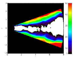
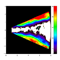
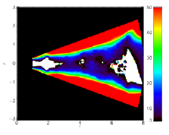
Figure 2: The ratio of the wavelength of the most rapidly growing MRI mode $\lambda_{m}$ to the local cell spacing $\Delta$ defined in the text. From left to right, the different panels show results from models S1a, S1b and S2. Any region coloured white has $\lambda_{m}/\Delta<5$, indicating that the fastest growing mode of the MRI is not well resolved there.

The picture presented above is true for all our simulations in their early phases. However, when designing useful and accurate stratified and turbulent protoplanetary disc models, several issues need to be addressed before presenting any detailed scientific results.

Figure 3: Time history of the toroidal magnetic flux $F_{\phi}(\theta_{0},t)$ threading the disc, normalized by its value at $t=0$, obtained in model S2. The solid line corresponds to $\theta_{0}=0.3$, the dotted line to $\theta_{0}=0.2$ and the dashed line to $\theta_{0}=0.1$. All of them show that the flux is expelled out of the midplane of the disc toward its corona.

The duration of the models themselves is one of them. In global cylindrical simulations, Papaloizou & Nelson (2003) demonstrated that long integration times, over several hundred orbits are required for the angular momentum transport quantities to reach meaningful saturated values. This is why, in this paper, we ran each model for at least $450$ orbits, and in some cases in excess of 600 orbits. In the following, we will show that this is sufficient to reach a steady state in the underlying disc structure, which is established after between $250$ to $500$ orbits.

A second issue is to determine the minimum resolution required to allow such models to maintain turbulence over long run times. To do so, we present here the results of models S1a and S1b. They were respectively run with GLOBAL and NIRVANA and have a resolution $(N_{r},N_{\phi},N_{\theta})=(272,90,126)$, corresponding to $15$ grid cells per scale height in the vertical direction ($\simeq 8$ zones per scale height in the azimuthal direction, $\simeq 3$ zones per scale height in the radial direction at the disc inner edge and $\simeq 22$ zones per scale height at the disc outer edge). Being identical in their set-up, these two models are also useful as a direct comparison between the two codes. For both cases, we find that the MRI grows leading to fully developed MHD turbulence and outward angular momentum transport.

The time history of $\langle\alpha_{M}\rangle$ is shown in figure 1 for model S1a (solid line) and S1b (dashed line). The two curves show very good agreement overall. This simply indicates that GLOBAL and NIRVANA give very similar results for the same problem. It is therefore meaningful to compare the results obtained by the two codes when they use different starting conditions and physical parameters. However, the slow decrease of $\langle\alpha_{M}\rangle$ with time in both models shows that MHD turbulence is getting weaker as the simulations proceed. No steady state seems to be reached in these simulations, apparently because the resolution used in models S1a and S1b is insufficient for vigorous MHD turbulence to be sustained in long runs. Indeed, in order to maintain turbulence, the simulations must be capable of resolving the unstable modes of the MRI. The critical wavelength for instability is given by (Balbus & Hawley 1991):

$$\lambda_{c}=\frac{2\pi}{\sqrt{3}}\frac{v_{A}}{\Omega}$$ (22)

and the wavelength of the fastest growing mode is

$$\lambda_{m}=2\pi\sqrt{\frac{15}{16}}\frac{v_{A}}{\Omega},$$ (23)

where $v_{A}$ is the Alfvén speed defined by

$$v_{A}=\sqrt{\frac{B^{2}}{4\pi\rho}}\,.$$ (24)

A simulation must have at least 5 grid cells per wavelength $\lambda_{m}$ for the fastest growing mode to be resolved (e.g. Hawley et al. 1995; Miller & Stone 2000). Figure 2 shows a contour plot in the ($r$, $\theta$) plane which displays the ratio $\lambda_{m}/\Delta$ for models S1a, S1b and S2. Here $\Delta$ is the local cell spacing (the diagonal distance between cell vertices along a path that passes through the cell centre). $\lambda_{m}$ is calculated from azimuthally and temporally averaged values of the magnetic field, $B$, and density $\rho$. The time averages were performed between the 500^th and 600^th orbit of models S1a and S1b. Regions of figure 2 which are coloured white correspond to regions where $\lambda_{m}/\Delta\leq 5$. It is clear that the MRI modes with wavelengths between $\lambda_{c}$ and $\lambda_{m}$ are not well resolved in these models around the midplane, leading to the weak and declining angular momentum transport shown in figure 1.

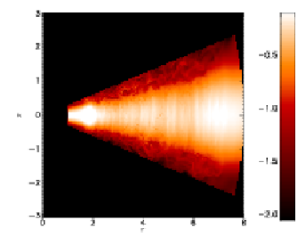
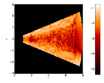
Figure 4: The left panel shows the logarithm of the density distribution in the ($r$, $\theta$) plane for model S2. Before taking the logarithm we transformed $\rho$ using the following: $\rho\rightarrow\rho\times r^{1.3}\times\exp{\left[Z^{2}/(2\times 0.07^{2})\right]}\times\exp{\left[-Z^{2}/(2\times 0.1^{2})\right]}$. This was done to increase the contrast in the figure. The right panel shows the logarithm of the Alfvén speed in the $(r,\theta)$ plane, obtained in model S2 after $400$ orbits.

Motivated by these results, we increased the resolution by a factor of $5/3$ to $25$ vertical grid cells per scale height. This translates into a resolution $(N_{r},N_{\phi},N_{\theta})=(455,150,213)$. As we demonstrate in section 4.2, the results of this model, labelled S2, suggest that a steady state is reached after about $300$ orbits (see for example figure 5) for this larger resolution. The rate of angular momentum transport seems to saturate, giving a saturated value of $\langle\alpha\rangle\sim 4\times 10^{-3}$ for the remainder of the simulations. A contour plot of $\lambda_{m}/\Delta$ for model S2 is shown in the right panel of figure 2, where $\lambda_{m}$ was time averaged between the 350^th and 450^th orbits. It is clear that $\lambda_{m}$ is well resolved throughout the disc in this model, leading to the turbulence being sustained. The value of $\lambda_{m}$ in the corona exceeds the total disc model thickness of $\simeq 8.5H$ for values of $|\theta-\pi/2|>3H/R$, such that the corona is stable against the MRI. In the rest of this paper we will describe results of models obtained using the same resolution as model S2. Unfortunately, this leads to very long computing times, at the limit of present day capacities: on standard Pentium 2.8GHz Xeon chips each model requires about 50000 CPU hours, or $\sim 6$ CPU years. Of course, it is still possible that MHD turbulence dies on time scales of several hundreds of orbits even for this large resolution, but the limited computational power available at the present time prevents running them for longer than about $500$ orbits. It is probably also the case that these simulations have not reached full numerical convergence. Figure 2 indicates that the smaller wavelength unstable modes $\sim\lambda_{c}$ are at best marginally resolved in model S2, such that a larger resolution may allow these modes to be more active. Nevertheless, the saturated state we generally obtained for the last $200$ to $300$ orbits sustains turbulence well enough to extract meaningful diagnostics describing the structure of the disc.

It is rather surprising that model S1a and S1b fail to show sustained MHD turbulence, as the resolution used is similar to that used by Nelson (2005) and Fromang & Nelson (2005), who reported sustained turbulence in cylindrical disc models initiated with net flux toroidal magnetic fields. This is because the magnetic field is trapped in the midplane of the disc in these cylindrical models while it is expelled to the coronae and out of the computational domain through the open boundaries in the stratified models presented in this paper. To illustrate this result, we plot in figure 3 the time history of the toroidal magnetic flux $F_{\phi}$ as obtained in model S1a. It is defined as

$$F_{\phi}(\theta_{0},t)=\int_{-\theta_{0}}^{\theta_{0}}\int_{R_{in}}^{R_{out}}B_{\phi}(r,0,\theta,t)rdrd\theta\,,$$ (25)

and in figure 3 is normalized by its initial value $F_{0}=F_{\phi}(\theta_{0},0)$. The different curves in this figure corresponds to $\theta_{0}=0.3$ (solid line), $\theta_{0}=0.2$ (dotted line) and $\theta_{0}=0.1$ (dashed line). All decrease from $1$ to small values during the first $100$ orbits (which corresponds to the growth of the MRI throughout the whole disc) and then oscillate around zero. This behavior shows that the magnetic flux is gradually expelled from the midplane toward the corona of the disc and out of the computational domain (the delay shown by the solid line to decay adds further weight to this conclusion). The oscillations between positive and negative values indicate that the adopted (vertical) boundary conditions allow azimuthal net flux into the domain, although essentially zero poloidal net flux enters. In the midplane of the disc, the amplitude of the oscillations is about $20-30\%$. After about $150$ orbits, the disc midplane essentially behaves as if MHD turbulence had been initiated using a zero net flux toroidal magnetic field. This requires a larger numerical resolution for the turbulence to be sustained over large periods (see the discussion by Nelson 2005) and explains why models S1a and S1b fail to reach a saturated state while cylindrical models using an equivalent resolution do.

4.2 The fiducial run – model S2

We describe in this section the general properties of model S2, which was run for $500$ orbits. As described above, the MRI grows in the first $100$ orbits, before developing into MHD turbulence, which then diffuses over the entire computational box (except for the buffer zones described in section 3.1). The disc settles into a quasi–steady state after $250$ orbits for the remainder of the simulation. The structure of the disc after $400$ orbits is illustrated in figure 4. The left hand snapshot shows the distribution of the logarithm of the density in the $(r,\theta)$ plane and the right hand panel represents the logarithm of the Alfvén speed $v_{A}$. Strong radially propagating density waves are seen in the former, while the small scale structure of the Alfvén speed in the latter confirms the turbulent nature of the flow, and also shows that the disc forms a structure consisting of a turbulent, magnetically subdominant ‘core’ near the midplane where the Alfvén speed is small, and a magnetically dominant corona in the upper regions of the disc where the Alfvén speed is large.

4.2.1 Angular momentum transport

Figure 5: Time history of the volume averaged value of $\langle\alpha\rangle$ (solid line), $\langle\alpha_{M}\rangle$ (dashed line) and $\langle\alpha_{R}\rangle$ (dotted line) in model S2. After an initial evolution driven by the linear growth of the MRI between $0$ and $250$ orbits, the disc settles into a quasi steady state for the remaining part of the simulation during which $\langle\alpha\rangle\sim 0.004$.

Figure 6: Radial profile of $\alpha$ (solid line), $\alpha_{M}$ (dashed line) and $\alpha_{R}$ (dotted line) in model S2. The curves are time–averaged between $t=350$ and $t=450$ orbits.

In this section, we quantify the rate of angular momentum transport resulting from the MHD turbulence. It is measured by the sum of the Maxwell and Reynolds stresses, already discussed in section 2.1. The time history of $\langle\alpha\rangle$, $\langle\alpha_{M}\rangle$ and $\langle\alpha_{R}\rangle$ are plotted in figure 5 respectively with the solid, dashed and dotted lines. As reported before for global MHD disc simulations (Hawley 2000, 2001; Steinacker & Papaloizou 2002; Papaloizou & Nelson 2003), the Maxwell stress dominates over the Reynolds stress in the approximate ratio of 3:1. The rate of angular momentum transport saturates after $250$ orbits and shows an almost constant value of $\langle\alpha\rangle\sim 4\times 10^{-3}$ for the remainder of the simulation. This is very similar to results reported for zero–net flux numerical simulations of cylindrical discs which further support the conclusion that our stratified disc model behaves like a zero–net flux disc. Papaloizou & Nelson (2003) report values of $\langle\alpha\rangle$ in the range 0.002 to 0.005 for a suite of zero net flux cylindrical disc models, and model C1 achieves a saturated state with $\langle\alpha\rangle\simeq 0.002$. This slightly smaller value of $\langle\alpha\rangle$ is consistent with the smaller vertical resolution used in model C1 compared with the models presented by Papaloizou & Nelson (2003). The radial profile of the Maxwell and Reynolds stresses, normalized by $\bar{P}$, are represented in figure 6 respectively with the dashed and dotted line. The solid line simply represents $\alpha$, the sum of the two. As reported by Papaloizou & Nelson (2003), we found large fluctuations in snapshots of these quantities. The smooth profile shown in figure 6 results from an averaging between $350$ and $450$ orbits. We note that time averaged $\alpha$ profiles in global MHD simulations (including these) often show variations between a factor of 2 and 3 across the disc (see e.g. Papaloizou & Nelson 2003; Steinacker & Papaloizou 2002). The origin of these variations is not clear, but may be related to the fact that fluctuations in $\alpha$ anticorrelate with changes to the local density and pressure due to mass transport. Local variations in $\alpha$ may thus be reinforced. It is possible that these variations will decrease with longer run times as the system loses memory of its initial conditions.

4.2.2 Structure of the corona

Figure 7: Vertical profile of the Maxwell stress (solid line) and the Reynolds stress (dashed line) obtained in model S2. The results are time averaged between $350$ and $450$ orbits and in radius between $r=4$ and $r=5$. Both curves are normalized by the midplane pressure. A decrease of both stresses is apparent for $Z/H>3$.

Figure 8: Vertical profile of the radio $P_{mag}/P$ at $r=3.5$ obtained in model S2 (solid line, averaged between $350$ and $450$ orbits), model S3 (dashed line, averaged between $270$ and $310$ orbits), model S4 (dotted line, averaged between $500$ and $600$) and model S5 (dotted–dashed line, averaged between $500$ and $600$ orbits). For all models, the disc is composed of a weakly magnetised core and a corona where the field is close to equipartition. The differences between the different curves results from the boundary conditions and are further discussed in the text.

Figure 9: The time averaged values of $|B_{r}|/B$, $|B_{\theta}|/B$ and $|B_{\phi}|/B$ as a function of $\theta/(H/R)$ for model S5. This was obtained by time averaging for 100 orbits at radius $r=3.5$. The $\phi$ component of $B$ is represented by the solid line, the $r$ component by the dotted line, and the $\theta$ component by the dashed line.

The results described above regarding the volume integrated properties of angular momentum transport show little difference compared with zero–net flux cylindrical disc models. In this section, we detail the structure of the upper layers of the disc.

Figure 7 shows the vertical profile of the Maxwell (solid line) and Reynolds (dashed line) stresses, normalised by the midplane pressure. Both curves are averaged in space between $r=4$ and $r=5$ and in time between $t=350$ and $t=450$ orbits. In agreement with the results obtained in local disc simulations (Miller & Stone 2000), both are fairly constant for $|Z|<2.5H$ before decreasing in the upper layers of the disc. This change is due to the establishment of a strongly magnetised corona. This is illustrated by figure 8, which shows the vertical profile of the ratio $P_{mag}/P$ at $r=3.5$ (the solid line corresponds to model S2). Simulation data were averaged in time between $350$ and $450$ orbits to smooth out the turbulent fluctuations (the other curves represented in figure 8 plot the results of models S3, S4 and S5 and will be discussed later). The relative strength of the magnetic field increases with $Z$, approaching equipartition in the neighborhood of the lower and upper boundaries. Even though the flow in the corona is not unstable to the MRI, we found it to be highly dynamic, exhibiting strongly time–dependent behaviour. Nevertheless, the structure of the corona is quite different to that in the midplane, with much smaller scale magnetic field fluctuations near the equatorial plane than in the corona of the disc. To try to quantify the topology of the field in the disc, figure 9 shows the variation of $|B_{r}|/B$, $|B_{\phi}|/B$, and $|B_{\theta}|/B$ versus $Z/H$, where $B=\sqrt{B_{r}^{2}+B_{\theta}^{2}+B_{\phi}^{2}}$. This plot corresponds to a radial location $r=3.5$ and was obtained by time averaging for 100 orbits between $t=350$ and $450$ orbits. It shows that the magnetic field topology is dominated by the azimuthal component of the field, as expected because of the strong Keplerian shear. However, as one moves away from the midplane toward the disc surface, there are some indications that the $r$ and $\theta$ component of the field become more important as their relative magnitude increases by about a factor of two. We comment here that the boundary conditions imposed on the magnetic field at the upper and lower disc surfaces were zero gradient outflow conditions.

4.2.3 Velocity and density fluctuations

Figure 10: Radial profile of the velocity fluctuations obtained in model S2. The curves, time–averaged between $t=350$ and $t=450$ orbits, correspond to radial (solid line), azimutal (dashed line) and vertical (dotted line) velocity fluctuations.

Figure 11: Vertical profile of the velocity fluctuations obtained in model S2 at $r=4.5$. The curves, time–averaged between $t=350$ and $t=450$ orbits, correspond to radial (solid line), azimutal (dashed line) and vertical (dotted line) velocity fluctuations.

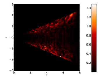
Figure 12: Snapshots of the Mach number $M_{s}$ in the $(r,\theta)$ plane at $t=450$ orbits obtained in model S2. Motions in the bulk of the disc are largely subsonic while weak shocks (with $M_{s}$ between $1$ and $1.5$) can be seen in its corona.

It is of interest to look at the velocity and density fluctuations generated by the turbulence in these models. Within the context of planetary formation, they affect the evolution of dust particles (Fromang & Papaloizou 2006), whose spatial distribution is important for the observational properties of protoplanetary discs, as well as the orbits of larger bodies such as boulders, planetesimals and protoplanets (Nelson & Papaloizou 2004; Nelson 2005; Fromang & Nelson 2005).

Figure 13: Normalised frequency distribution of the relative density fluctuations in models S2 (solid line), S5 (dashed line), C1 (dot–dashed line) and C2 (dotted line). All curves are averaged in time for 100 orbits. Results obtained in run S2 and S5 are averaged in the volume $|Z|<H$ and $3<r<5$. Results obtained for runs C1 and C2 are averaged over the entire vertical extend and in radius between $r=3$ and $r=5$ for model C1, and between $r=2.5$ and $r=4$ for model C2. The curves for runs S2, S5 and C1 have a similar width, while model C2 produces a wider distribution because it contained a net flux magnetic field.

Figure 10 shows the radial profile of the velocity perturbations obtained in model S2, averaged between $t=350$ and $t=450$ orbits. The solid, dashed and dotted line respectively represents the radial, azimuthal and vertical velocity perturbation, normalized by the local sound speed and averaged in space within $H/2$ around the disc midplane. Typically, these fluctuations are all of the order of a few percents of the sound speed. This is slightly smaller than previous results obtained in the shearing box (Stone et al. 1996; Fromang & Papaloizou 2006), who found values of the order of $10\%$. There is a marked tendency for the radial fluctuations to be larger, by about a factor of two, than the azimutal and vertical fluctuations. This is due to the presence of density waves travelling radially through the disc. This is also seen in local boxes but its effect is less pronounced in that case. The vertical profiles of the fluctuations are shown, using the same conventions, in figure 11. As noted by Miller & Stone (2000) and Turner et al. (2006) who presented shearing box calculations, they increase in the upper layers of the disc, where the averaged Mach number reaches $0.4$. This increase in perturbed velocities arises because disturbances that are excited near the high density midplane increase in amplitude as they propagate vertically into the lower density regions, due to conservation of wave action. In addition, the increasing influence of the magnetic field with height means that propogating Alfvén waves in the disc corona can excite approximately sonic motions where the Alfvén speed exceeds the sound speed. The result is that shocks are generated in the upper regions of the disc, as illustrated by figure 12 which shows a snapshot in the ($r$, $\theta$) plane of the perturbed velocity divided by the sound speed. Weak shocks, for which $M_{s}$ reaches $1.5$, are visible on this image.

The normalised frequency distribution for the density fluctuations is shown in figure 13 for model S2 (solid line). The results of the simulations were averaged in time between $350$ and $450$ orbits in order to smooth out the turbulent fluctuations. An additional spatial averaging was performed in the volume $3<r<5$ and $|Z|<H$. The results show that the distribution is approximately Gaussian with standard deviation $\sigma_{\rho}\simeq 0.08$. This result agrees well with those of models S5 (dashed line) and C1 (dot–dashed line), showing that neither the boundary conditions nor the stratification have a strong impact on the amplitude of the turbulent density fluctuations near the midplane. However, the results of model C2, shown with the dotted line, produce a broader distribution ($\sigma_{\rho}\simeq 0.13$). This is because the toroidal net flux is nonzero in this model, while it vanishes in model S2, S5 and C1. This results in a stronger MHD turbulence, along with slightly larger density fluctuations. It is already known that these density fluctuations may be responsible for driving stochastic migration of low mass planets and planetesimals (e.g. Nelson & Papaloizou 2004; Nelson 2005), and this effect will be explored in more detail in a forthcoming paper within the context of stratified, turbulent disc models.

4.3 The effect of the boundary conditions in $\theta$

We now present the results of simulations designed to test the role of the vertical boundary conditions we have adopted. We begin by examining a model whose vertical domain is larger than model S2 but otherwise similar, and then describe a model with periodic boundary conditions in the vertical direction.

4.3.1 A larger vertical domain – model S3

Figure 14: Time history of the Maxwell stress in model S2 (solid line) and S3 (solid line). The latter has a larger vertical extent. The good agreement between the two curves shows that the boundary conditions and vertical extent have little effect on the results of model S2.

We first focus on model S3. Compared to model S2 described above, it has an extended domain in $\theta$: $|\theta-\pi/2|\leq 0.4$. This corresponds to a total of $5.7$ scale heights on both side of the equatorial plane. For the actual resolution to remain the same, the total number of grid cells was increased to $(N_{r},N_{\phi},N_{\theta})=(455,150,285)$. All the other parameters of model S3 are otherwise identical to those of model S2. Note however that the larger number of cells increased the computing time of model S3. As a result it was run for only $325$ orbits.

Figure 14 compares the time history of $\langle\alpha_{M}\rangle$ in model S2 (solid line) and in model S3 (dashed line). Both curves show similar evolution. Moreover, model S3 starts to saturate after about $270$ orbits at a level that is comparable to that of model S2. Figure 8 also shows the vertical profile of $P_{mag}/P$ (dotted line), averaged between $270$ and $310$ orbits. It shows that model S2 and S3 agree very well in the bulk of the disc.

These results demonstrate that the structure of the discs described so far are not affected strongly by the boundary conditions and vertical extent of the computational domain.

Figure 15: Time evolution of the volume averaged stress parameter $\langle\alpha_{M}\rangle$ for model S4 (solid line) and S2 (dashed line). Despite the different boundary conditions, the two models display similar time history for the angular momentum transport properties.

Figure 16: The time evolution of the azimuthal magnetic flux for model S4, normalised to its initial value. The dashed line shows the total flux within an angular distance $|\theta-\pi/2|\leq H/R$ above and below the midplane. The dotted line shows the flux within an angular distance $|\theta-\pi/2|\leq 2H/R$ above and below the midplane. The solid line shows the flux throughout the whole disc, and varies with time due to the imperfect nature of the periodic boundary conditions adopted in the meridional direction.

4.3.2 Periodic boundary conditions – model S4

We have computed one model, run S4, which uses periodic boundary conditions in the vertical direction (i.e. $\theta$–direction). Clearly this is not a realistic boundary condition to use for an accretion disc, but it nonetheless provides a test of the role that the vertical boundaries play in these simulations. Before describing the results of the simulation in detail, we first comment that the periodicity condition implemented in the NIRVANA (or GLOBAL) code is imperfect when applied in the meridional direction. This is because the physical sizes of the cells that overlap at the top and bottom of the disc are different. The effect of this is small, but one manifestation is that magnetic flux is not conserved as it passes through the upper surface of the disc and re-enters through the lower surface (and vice versa). As shown below, this causes a 5 % decrease in magnetic flux in the domain over the simulation run time.

Figure 17: A slice plotted in the ($r$, $\theta$) plane of the disc showing the logarithm of the Alfvén speed for model S4. Comparing with similar plots for models S2 (figure 4) and S5 (figure 22) shows that the trapping of magnetic flux in the upper disc regions of model S4 leads to an elevated value of the Alfvén speed there.

The time evolution of the volume averaged $\langle\alpha_{M}\rangle$ value is shown in figure 15 for model S4 (solid line) and compared to model S2 (dashed line). The early rise and fall of this quantity is similar in both models. One feature of the runs that appears throughout this paper is that the time required for saturation of the turbulence is longer for the NIRVANA simulations than for the GLOBAL ones. Nonetheless the final states that are reached are very similar in each case. Inspection of figure 15 shows that during the time interval 350–550 orbits, short duration outbursts are observed in the $\alpha_{M}$ values. This phenomenon seems to be explained by figure 16, which shows the time evolution of the azimuthal magnetic flux in the computational domain defined by equation (25). The solid line shows the total flux in the domain, and because of the periodicity of the vertical boundaries this is approximately conserved (the small non conservation was explained above). The dashed and dotted lines show the magnetic flux in the disc below heights $|\theta-\pi/2|<H/R$ and $|\theta-\pi/2|<2H/R$, respectively. As described for model S2, the onset of the MRI and turbulence causes the magnetic flux to rise up through the disc to form a magnetically dominated corona. In model S4 this magnetic flux is effectively trappped in the disc and is able to build up to large values in the corona. Figure 16 shows that substantial flux occassionally comes down from the corona into the turbulent core, within $\sim 2H/R$ of the midplane, where its presence causes an episodic increase in turbulent activity.

The effects of trapping the magnetic flux in the domain on the evolution of the disc is illustrated by figure 17 which shows a snapshot of the Alfvén speed plotted as a slice in the ($r$, $\theta$) plane. The contrast in the Alfvén speed between the inner disc core and the upper corona is much greater in this case than was observed for model S2 because the magnetic field in the upper regions is larger. This is further illustrated by figure 8 which shows the ratio of magnetic to thermal pressure $P_{mag}/P$ as a function of disc height for model S4 using the dotted line. This plot corresponds to $r=3.5$ and was obtained by time averaging between $t=500$ and $t=600$ orbits. It is clear that the corona in this case is highly dominated by the magnetic field, with $P_{mag}/P\simeq 30$ near the disc surface, in contrast to the value of $P_{mag}/P\simeq 1$ obtained in model S2.

One effect of these large magnetic field and Alfvén speed values is that large supersonic motions are generated in the disc corona. This is illustrated by figure 18 which shows a snapshot of the velocity perturbation divided by the local sound speed, projected onto the ($r$, $\theta$) plane. Strong shocks can be seen in the upper disc surface with Mach numbers $M_{s}$ in excess of 10 being common. This is in contrast to the more quiescent state of the corona obtained in model S2 where Mach numbers between 1 – 2 are observed. We note that $M_{s}\sim 10$ indicates that the maximum gas velocities in the corona are basically given by the Alfven speed limiter $v_{A}^{c}$ (which is roughly ten times the sound speed). This is probably a numerical consequence of the particular value chosen for $v_{A}^{c}$. However, the exact strength of these shocks is not of crucial importance since they are mostly a consequence of the unphysical periodic boundary conditions, which serve to illustrate the effect of trapping the toroidal net flux on the structure of the corona.

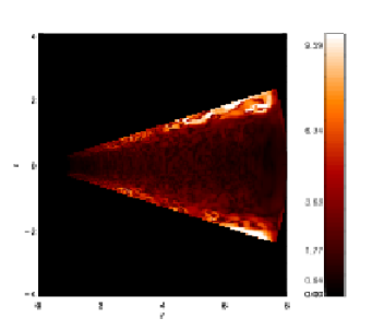
Figure 18: Snapshot of velocity fluctuations in the disc normalised to the local sound speed, plotted in the ($r$, $\theta$) plane. It is clear that strong shocks (Mach numbers $>10$ ) are generated in the upper disc regions due to the large magnetic forces there.

4.4 A thicker disc – model S5

We now present the results of run S5 whose parameters are described in table 1. This run used a thicker disc with $H/R=0.1$, and a correspondingly smaller number of grid cells ($N_{r}$, $N_{\phi}$, $N_{\theta}$)=(360, 120, 210). A distinct advantage of using a thicker disc is that in principle it allows the use of a smaller number of grid cells while still giving rise to a resolved model. We remind the reader that model S5 used a “viscous outflow boundary condition” at the inner edge of the computational domain (see section 3.1 for details).

4.4.1 Global disc properties

Figure 19: Time history of the stress parameter $\langle\alpha\rangle$ for model S5. The dotted line shows the contribution from the Maxwell stress, the dashed line shows the contribution from the Reynolds stress, and the solid line shows the sum of these.

Figure 20: Time history of the azimuthal magnetic flux for model S5. The dot-dashed line shows the normalised magnetic flux contained within $|\theta-\pi/2|\leq H/R$ about the midplane, the dashed line shows the flux within $|\theta-\pi/2|\leq 2H/R$, the dotted line shows the flux within $|\theta-\pi/2|\leq 3H/R$ and the solid line corresponds to the magnetic flux within the whole disc. As for model S2, the initial flux within the disc escapes through the upper and lower disc surfaces leading to a substantial reduction throughout the disc. In particular, the regions around the midplane tend towards a state of zero net flux. Oscillations in the total magnetic flux are caused by magnetic flux entering through the vertical boundaries.

The early evolution of this model proceeds very much along the lines discussed in the opening paragraph of section 4. The time evolution of the volume averaged viscous stress parameter $\langle\alpha\rangle$ is presented in figure 19, and shows that it saturates at a value of $\langle\alpha\rangle\simeq 4\times 10^{-3}$ after 500 orbits, in basic agreement with the models S2, S3, and S4. The time evolution of the azimuthal magnetic flux defined by equation (25) is shown in figure 20. Similar behaviour is seen in model S5 as was described for run S2, with magnetic buoyancy causing the initial flux to rise vertically through the disc into the corona where it escapes through the open boundary. Close inspection of the dot-dashed line in figure 20 shows that the disc near the midplane contains essentially zero net magnetic flux after about 100 orbits, such that sustained MHD turbulence there requires the action of a dynamo. As already described, this feature of these simulations adds to the computational burden as zero net flux simulations require high resolution in order that numerical resistivity does not quench the MRI. The solid line in figure 20 shows the total flux in the whole computational domain. The fact that it oscillates about the zero line indicates that the adopted boundary conditions lead to magnetic flux entering the computational domain. The relatively small amount of flux that enters suggests that this feature does not dramatically alter the results of our simulations.

Figure 21 shows snapshots of the density in the disc after 500 orbits. The left panel shows the density in the disc midplane, and the right panel shows a vertical slice through the ($r$, $\theta$) plane. The radial transport of mass during the simulation has caused a shallow depression to form in the density profiles at radii between $5\leq r\leq 7$ which are apparent in the figure. Also apparent are the trailing spiral waves excited by the turbulence. These propagate radially through the model and, because the disc is isothermal in the vertical direction, these waves propagate with little vertical structure. Animations of the disc density projected onto the ($r$, $\theta$) plane indicate that individual prominent spiral waves which propagate radially occupy most of the vertical extent of the disc. Comparison between figures 21 and 4 shows that the ‘viscous outflow’ boundary condition at the inner edge of the disc is having the desired effect of preventing a substantial build–up of mass there. As we comment in section 4.4.3, some build–up of mass near the inner boundary does occur in this model because the chosen value of the outflow velocity was too small, but this should be a simple problem to remedy in future models.

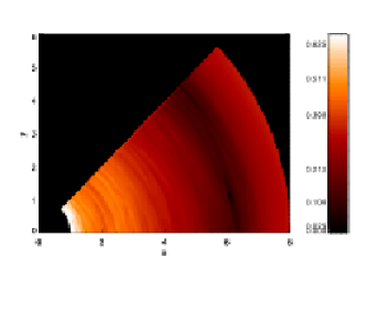
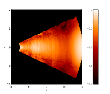
Figure 21: The left panel shows an image of the density at the disc midplane after 500 orbits for model S5. The right hand panel is a slice plotted in the $(r,\theta)$ plane showing the vertical density profile (this panel shows the logarithm of the density after performing a transformation of $\rho$ similar to that described in the caption of figure 4). These images show that the action of the stresses have caused signification mass transport within the disc, resulting in an apparent density depression at $r\sim 6$.

Figure 22 presents a vertical slice projected onto the ($r$, $\theta$) plane showing the logarithm of the Alfvén speed. As observed in the runs S2 and S4, the Alfvén speed noticeably increases as one moves away from the midplane to the disc surface above a height of about $2H$. It is also clear from this figure that the disc is magnetically active all the way down to the inner radial boundary due to the ‘viscous outflow’ condition used in this model. The increase in relative strength of the magnetic field with height is also illustrated by figure 8 where the ratio of magnetic pressure to gas pressure is plotted as a function of $\theta$ at radius $r=3.5$ using the dot–dashed line. In agreement with the results of model S2, one sees that $P_{mag}/P\simeq 0.01$ within $|\theta-\pi/2|<2H/R$, but it quickly rises to $P_{mag}/P\simeq 0.5$ in the low density regions above the midplane.

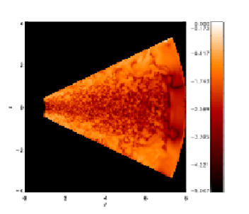
Figure 22: This figure shows the logarithm of the Alfvén speed in the disc after 500 orbits obtained by plotting a slice in the $(r,\theta)$ plane.

The variation of stress with height is shown in figure 23, which shows a similar fall–off in the Maxwell and Reynolds stresses with height as observed for model S2. This figure corresponds to radius $r=3.5$, and was obtained by time averaging the stresses for 100 orbits.

Figure 24, which should be compared with figure 9, shows the variation of $|B_{r}|/B$, $|B_{\phi}|/B$, and $|B_{\theta}|/B$ versus $\theta$. This plot corresponds to radial location $r=3.5$ and was obtained by time averaging for 100 orbits between $t=500$ – 600 orbits. It shows a bigger increase of the $r$ and $\theta$ component of the field in the upper layers of the disc than in model S2. This is clearly influenced by the boundary conditions imposed at the disc surface, where the field is defined to be normal to the boundary with magnitude defined by the $\nabla.\mbox{\boldmath{$B$}}=0$ condition in the NIRVANA runs (e.g. Hawley 2000), but, as suggested by the results of model S2 (which show a similar but reduced effect with different boundary conditions), it is probably also due to the vertical stretching of field lines as localised regions of magnetised fluid rise up from the disc midplane.

4.4.2 Velocity and density fluctuations

The ratios of the velocity fluctuations in the $r$, $\theta$, and $\phi$ directions to the local sound speed were calculated and found to be in very good agreement with the results of run S2 plotted in figure 11. The increase of the velocity perturbation Mach number as one moves from the midplane to the disc surface results in weak shocks being generated in the corona, as illustrated by figure 25 which shows a snapshot in the ($r$, $\theta$) plane of the perturbed velocity divided by the sound speed. As observed in model S2, and unlike model S4, typical Mach numbers for these shocks range between 1 – 3. The fact that model S4 showed much stronger shocks illustrates the role that magnetic forces in the corona have in exciting these supersonic motions.

Figure 23: The time averaged values of the Maxwell stress (solid line) and Reynolds stress (dotted line), normalised to the midplane pressure, as a function of $\theta$ for model S5. This was obtained by time averaging for 100 orbits at radius $r=3.5$. This figure is similar to that obtained for model S2, showing a similar drop-off of stress with height.

Figure 24: Same as figure 9. As in model S2, the azimuthal component remains dominant throughout the vertical domain, but the field topology changes near the disc surface where the $\theta$ and $r$ components become larger.

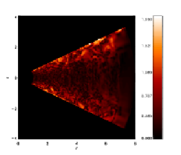
Figure 25: Snapshots of the velocity fluctuations normalised by the local sound speed obtained in model S5. The results agrees very well with those of model S2 (see figure 12)

The distribution of the density fluctuations in model S5 is represented in figure 13 with the dashed line. Simulation data were averaged in time between $500$ and $600$ orbits, and in space in the radial interval $3<r<5$ and in the height interval $|\theta-\pi/2|<H/R$ to obtain this curve. Once again, the results are in very good agreement with those of model S2.

4.4.3 Mass flow in the disc

Once model S5 had completed just over 600 orbits it was stopped. It was restarted again at the 500 orbit mark, but with its density field and azimuthal velocity reset to the values they had initially at time $t=0$. All other variables (e.g. magnetic field, vertical and radial velocities) had the values corresponding to the 500 orbit mark of the S5 run. This procedure was undertaken to smooth out the large variations in surface density that arise during the early stages of these simulations because the stresses have large radial and temporal variations during these times. The aim is to generate a turbulent protoplanetary disc with simple surface density structure as a function of radius.

Having restarted the model it was run for 55 orbits, at which point time averaging of the state variables and stresses within the disc were commenced. The simulation was continued for a further 100 orbits while the time averaging was performed.

The radial variation of the time averaged $\alpha$ values in the disc are shown in figure 26. The results are similar to those obtained in model S2. We note here, however, that the value of $\alpha$ is small ($\sim 10^{-4}$) near the disc inner radial boundary where a ‘viscous outflow’ condition is imposed on the radial velocity. This arises because during the initial phases of the run for model S5, the magnetic field was non zero only in the range $2.5\leq r\leq 6$. As turbulence develops, mass and magnetic field are transported inward, but at a rate which is larger than accounted for by the ‘viscous outflow’ condition. The density in the midplane thus increases in this region, such that the unstable modes of the MRI remain small and unresolved here [see equation (22)]. Consequently turbulence in the inner most region of the disc remains weak. A remedy for this would be to modify the ‘viscous outflow’ condition so that it responds more accurately to the inflow of matter from further out rather than using a prescribed inward velocity as was done for model S5.

Figure 26: Radial variation of the time averaged value of $\alpha$ for model S5. The curves were obtained by time averaging between 500–600 orbits. The dashed line corresponds to the Maxwell stress, the dotted line to the Reynolds stress, and the solid line to the sum of these.

Figure 27 shows the time averaged radial mass flux through the disc as a function of radius. Each line corresponds to mass flow at a different height in the disc. The dotted line corresponds to the region within $\Delta\theta\leq H/R$ about the midplane, where $\Delta\theta=|\theta-\pi/2|$. The dashed line corresponds to the region bounded by $H/R<\Delta\theta\leq 2H/R$, the dot–dashed corresponds to $2H/R<\Delta\theta\leq 3H/R$, and the dot-dot-dot-dashed line corresponds to $3H/R<\Delta\theta\leq(\theta_{max}\,\,{\rm or}\,\,\theta_{min})$. The total radial mass flux is shown by the solid line (and is the sum of all the other lines). Evidently negligible mass is transported in the upper most parts of the disc corona, as there is very little mass there. The other three regions considered, however, all contribute significantly to the mass flux. In the outer regions of the disc the zone near the midplane appears to be transporting mass inward whereas the upper regions of the disc are transporting it outward, suggesting that the long term mass flow in vertically stratified turbulent discs can be a complicated function of disc height. A similar picture was described by De Villiers & Hawley (2003) for simulations of accretion tori around black holes.

The total vertical mass flux through both boundaries at the disc surface is shown in figure 28. It is clear that the disc drives a vertical mass flow at a rate that is less than two orders of magnitude below that which occurs radially in the disc. A similar result was obtained in model S2. However, the restricted size of our meridional domain prevents us from commenting in detail about any wind that may be launched from the disc surface.

We now turn to the question of how well the averaged radial velocity in the disc agrees with the expectations of thin disc theory as described by equation (15). We computed the time average of $\Sigma(R)$, ${\overline{T}_{M}}(R)$, ${\overline{T}_{R}}(R)$ and using a simple finite difference approximation calculated the expected radial velocity profile ${\overline{v}_{R}}$ in the disc. The results are shown using the dotted line in figure (29), where the actual value of ${\overline{v}_{R}}$ obtained in the simulation is shown using the solid line. Although the effect of fluctuations remain, the agreement between the predicted and actual values is remarkably good. This demonstrates that the vertically stratified turbulent discs considered here behave very much like standard $\alpha$ discs when their evolution is considered over long time scales. On short time scales, however, the differences are self–evident. We note that a comparison of the predicted and actual values of ${\overline{v}}_{R}$ was undertaken for model S4 and gave rise to a very similar level of agreement.

Figure 27: Radial mass flux versus radius for model S5. The dotted line corresponds to $|\theta-\pi/2|\leq H/R$, the dashed line corresponds to $H/R<|\theta-\pi/2|\leq 2H/R$, the dot-dashed line corresponds to $2H/R<|\theta-\pi/2|\leq 3H/R$, and the dot-dot-dot-dashed line corresponds to $3H/R<|\theta-\pi/2|\leq$ disc surface. The solid line represents the total radial mass flux through the disc.

5 Conclusions

In this paper we have presented the results of 3-D MHD simulations of stratified and turbulent protoplanetary disc models. Our primary motivation is to develop disc models that can be used to examine outstanding issues in planet formation such as the migration of protoplanets, the growth and settling of dust grains, gap formation and gas accretion by giant planets, and the evolution and influence of dead–zones. Given that these phenomena occur on secular time scales, a key requirement is the development of disc models which are able to achieve a statistical steady state and sustain turbulence over long run times.

We examined the issue of numerical resolution, and found that disc models with $\simeq 15$ vertical zones per scale height in the vertical direction showed a continuing slow decline in their magnetic activity, and gave rise to relatively small values of $\langle\alpha\rangle$. A suite of higher resolution runs with $\simeq 25$ zones per scale height achieved statistical steady states with values of $\langle\alpha\rangle\simeq 4\times 10^{-3}$, and it was shown that these models resolve the fastest growing modes of the MRI throughout the disc once a turbulent steady state has been achieved. For this reason we focused on simulations performed using this higher resolution.

Figure 28: The sum of the mass fluxes through the vertical boundary of the disc located at $\theta=\theta_{max}$ and $\theta_{min}$.

The key features of the resulting disc models are:

• Any toroidal magnetic flux that is initially present within the disc is quickly expelled from the midplane due to magnetic buoyancy. This occurs on a time scale of $\sim 100$ orbits, which is the time required for the MRI to grow and develop into non linear turbulence throughout the disc. The disc then evolves as if it is threaded by an approximately zero net flux magnetic field, such that high resolution is required to maintain turbulent activity.

• A quasi–steady state turbulent disc is obtained after run times of between 250 – 500 orbits, depending on the model. The volume averaged value of the effective viscous stress paramater $\langle\alpha\rangle\simeq 4\times 10^{-3}$, and time averaged radial profiles of $\alpha$ yield variations of no more than a factor of two within the active domains of the disc models. These results are in basic agreement with previous studies of cylindrical discs (Hawley 2001; Papaloizou & Nelson 2003)

• The discs can be described as having a two–phase global structure as a function of height: a dense, magnetically subdominant turbulent core that is unstable to the MRI in regions within $|Z|<2.5H$ of the midplane, above and below which exists a highly dynamic and magnetically dominated corona which supports weak shocks and is stable against the MRI. The engine that drives this structure is the MRI which generates and amplifies magnetic field near the midplane, which then buoyantly rises up into the low density corona where it dissipates and flows out through the boundaries at the disc surface. This is in basic agreement with the shearing box simulations presented by Miller & Stone (2000) and recent studies of thick tori orbiting around black holes (Hawley 2000; Hawley & Krolik 2001; Hawley et al. 2001; De Villiers et al. 2003).

• The velocity and density fluctuations generated by the models were found to be smaller than those obtained in cylindrical disc simulations using toroidal net flux magnetic field configurations (Nelson 2005; Fromang & Nelson 2005). $\delta\rho/\rho_{0}\simeq 0.08$ in the stratified runs whereas in the cylindrical disc runs with net flux $\delta\rho/\rho_{0}\simeq 0.13$. This has implications for the dynamics of dust, planetesimals and low mass protoplanets in turbulent discs as their stochastic evolution is driven by these fluctuating quantities.

• The vertically, azimuthally and time averaged values of the radial velocity in some of the disc models were compared with the expectations of viscous disc theory, and were found to give very good agreement. We conclude that, subject to a suitable time average, global evolution of these stratified turbulent models is in good accord with standard viscous disc theory (e.g. Shakura & Sunyaev 1973; Balbus & Papaloizou 1999; Papaloizou & Nelson 2003)

Figure 29: Comparison between the time averaged radial velocity obtained in the simulations (solid line) and the predicted value of $v_{R}$ obtained from equation (15) shown by the dotted line.

There are a number of outstanding issues raised by our simulation results. Fromang & Nelson (2005) reported the presence of anticyclonic vortices in turbulent unstratified cylindrical disc models. In the stratified models we present in this paper, however, we did not find any evidence of vortices. This could be due to a number of reasons. First, the vertical stratification may prevent the formation of vortices near the midplane. A study by Barranco & Marcus (2005) showed that column–vortices in stratified discs are unstable and are quickly destroyed. They showed that vortices could form in the more strongly stratified upper regions of the disc which are more than one scale height above the midplane. In our simulations these regions are typically dominated by magnetic fields, whose associated stresses may prevent the formation of vortices there. Second, we adopted a smaller azimuthal domain than Fromang & Nelson (2005): $\pi/4$ versus $\pi/2$ and $2\pi$ models. This may prevent the formation of vortices, which were found to be quite extended in $\phi$ by Fromang & Nelson (2005). We did not observe any vortices in the cylindrical disc model C1 described in section 3.2, and this may be partly explained by the smaller azimuthal domain. Finally, the different magnetic field topology contained in the disc may play a role: Fromang & Nelson (2005) used a net flux toroidal magnetic field. In the stratified models, the toroidal flux is quickly expelled from the disc midplane and the evolution is more similar to that of a zero net flux disc. The cylindrical model C1 contained a zero net flux magnetic field. The properties of the field can affect the turbulence and hence the formation of vortices. In particular, stronger spatial and temporal variations in the stresses may cause the surface density variations to differ systematically between the models presented here and those in Fromang & Nelson (2005). If the formation of vortices in the models described in Fromang & Nelson (2005) are related to the ‘planet modes’ described by Hawley (1987), then these differences may explain the lack of vortices seen in the stratified models and model C1. These issues, and their influence on the evolution of solid bodies will be explored in greater detail in a future paper.

Finally, this is the first paper in a series which describes an approach to setting up models of turbulent, stratified protoplanetary discs capable of sustaining turbulence over long run times. Future papers will present a systematic study of outstanding problems in planet formation theory, such as disc–planet interactions, dust and planetesimal dynamics, and effects related to the presence of a dead zone. We also note that these models themselves can be further improved by including a realistic equation of state, heating and cooling of the disc, and a self–consistent treatment of the evolving ionisation fraction and conductivity of the disc material. At the present time inclusion of these physical processes is beyond current computational resources.

References

- Afshordi et al. (2005) Afshordi, N., Mukhopadhyay, B., & Narayan, R. 2005, ApJ, 629, 373
- Armitage (1998) Armitage, P. J. 1998, ApJ, 501, L189
- Balbus & Hawley (1991) Balbus, S. & Hawley, J. 1991, ApJ, 376, 214
- Balbus & Papaloizou (1999) Balbus, S. & Papaloizou, J. 1999, ApJ, 521, 650
- Barranco & Marcus (2005) Barranco, J. A. & Marcus, P. S. 2005, ApJ, 623, 1157
- Beckwith & Sargent (1996) Beckwith, S. V. W. & Sargent, A. I. 1996, Nature, 383, 139
- Blaes & Balbus (1994) Blaes, O. M. & Balbus, S. A. 1994, ApJ, 421, 163
- Brandenburg et al. (1996) Brandenburg, A., Nordlund, A., Stein, R. F., & Torkelsson, U. 1996, ApJ, 458, L45+
- De Villiers et al. (2003) De Villiers, J., Hawley, J. F., & Krolik, J. H. 2003, ApJ, 599, 1238
- De Villiers & Hawley (2003) De Villiers, J.-P. & Hawley, J. F. 2003, ApJ, 592, 1060
- Fromang & Nelson (2005) Fromang, S. & Nelson, R. 2005, MNRAS, 364, L81
- Fromang & Papaloizou (2006) Fromang, S. & Papaloizou, J. 2006, A&A, 452, 751
- Fromang et al. (2002) Fromang, S., Terquem, C., & Balbus, S. A. 2002, MNRAS, 329, 18
- Gammie (1996) Gammie, C. F. 1996, ApJ, 457, 355
- Hartmann et al. (1998) Hartmann, L., Calvet, N., Gullbring, E., & D’Alessio, P. 1998, ApJ, 495, 385
- Hawley & Stone (1995) Hawley, J. & Stone, J. 1995, Comput. Phys. Commun., 89, 127
- Hawley (1987) Hawley, J. F. 1987, MNRAS, 225, 677
- Hawley (2000) Hawley, J. F. 2000, ApJ, 528, 462
- Hawley (2001) Hawley, J. F. 2001, ApJ, 554, 534
- Hawley & Balbus (1991) Hawley, J. F. & Balbus, S. A. 1991, ApJ, 376, 223
- Hawley et al. (2001) Hawley, J. F., Balbus, S. A., & Stone, J. M. 2001, ApJ, 554, L49
- Hawley et al. (1995) Hawley, J. F., Gammie, C. F., & Balbus, S. A. 1995, ApJ, 440, 742
- Hawley et al. (1996) Hawley, J. F., Gammie, C. F., & Balbus, S. A. 1996, ApJ, 464, 690
- Hawley & Krolik (2001) Hawley, J. F. & Krolik, J. H. 2001, ApJ, 548, 348
- Ilgner & Nelson (2006) Ilgner, M. & Nelson, R. P. 2006, A&A, 445, 223
- Ioannou & Kakouris (2001) Ioannou, P. J. & Kakouris, A. 2001, ApJ, 550, 931
- Johansen et al. (2006) Johansen, A., Klahr, H., & Henning, T. 2006, ApJ, 636, 1121
- Kessler-Silacci et al. (2006) Kessler-Silacci, J., Augereau, J.-C., Dullemond, C. P., et al. 2006, ApJ, 639, 275
- Lissauer (1993) Lissauer, J. J. 1993, ARA&A, 31, 129
- Miller & Stone (2000) Miller, K. A. & Stone, J. M. 2000, ApJ, 534, 398
- Mukhopadhyay et al. (2005) Mukhopadhyay, B., Afshordi, N., & Narayan, R. 2005, ApJ, 629, 383
- Nelson & Papaloizou (2003) Nelson, R. & Papaloizou, J. 2003, MNRAS, 339, 993
- Nelson (2005) Nelson, R. P. 2005, A&A, 443, 1067
- Nelson & Papaloizou (2004) Nelson, R. P. & Papaloizou, J. C. B. 2004, MNRAS, 350, 849
- O’dell et al. (1993) O’dell, C. R., Wen, Z., & Hu, X. 1993, ApJ, 410, 696
- Papaloizou & Nelson (2003) Papaloizou, J. C. B. & Nelson, R. P. 2003, MNRAS, 339, 983
- Papaloizou et al. (2004) Papaloizou, J. C. B., Nelson, R. P., & Snellgrove, M. D. 2004, MNRAS, 350, 829
- Safronov (1969) Safronov, V. S. 1969, Evoliutsiia doplanetnogo oblaka. (1969.)
- Shakura & Sunyaev (1973) Shakura, N. I. & Sunyaev, R. A. 1973, A&A, 24, 337
- Sicilia-Aguilar et al. (2006) Sicilia-Aguilar, A., Hartmann, L., Calvet, N., et al. 2006, ApJ, 638, 897
- Sicilia-Aguilar et al. (2004) Sicilia-Aguilar, A., Hartmann, L. W., Briceño, C., Muzerolle, J., & Calvet, N. 2004, AJ, 128, 805
- Stauffer et al. (1994) Stauffer, J. R., Prosser, C. F., Hartmann, L., & McCaughrean, M. J. 1994, AJ, 108, 1375
- Steinacker & Papaloizou (2002) Steinacker, A. & Papaloizou, J. 2002, ApJ, 571, 413
- Stone et al. (1996) Stone, J. M., Hawley, J. F., Gammie, C. F., & Balbus, S. A. 1996, ApJ, 463, 656
- Stone & Norman (1992) Stone, J. M. & Norman, M. L. 1992, ApJS, 80, 753
- Turner et al. (2006) Turner, N. J., Willacy, K., Bryden, G., & Yorke, H. W. 2006, ApJ, 639, 1218
- Ziegler & Yorke (1997) Ziegler, U. & Yorke, H. W. 1997, Computer Physics Communications, 101, 54