Semi-empirical analysis of Sloan Digital Sky Survey galaxies
III. How to distinguish AGN hosts

Abstract

This paper considers the techniques to distinguish normal star forming (NSF) galaxies and active galactic nuclei (AGN) hosts using optical spectra. The observational data base is a set of 20 000 galaxies extracted from the Sloan Digital Sky Survey, for which we have determined the emission line intensities after subtracting the stellar continuum obtained from spectral synthesis. Our analysis is based on photoionization models computed using the stellar ionizing radiation predicted by population synthesis codes (essentially Starburst 99) and, for the AGNs, a broken power-law spectrum. We explain why, among the four classical emission line diagnostic diagrams, ([O iii]/H$\beta$ vs [O ii]/H$\beta$, [O iii]/H$\beta$ vs [N ii]/H$\alpha$ (the BPT diagram), [O iii]/H$\beta$ vs [S ii]/H$\alpha$, and [O iii]/H$\beta$ vs [O i]/H$\alpha$), the BPT one works best. We show however, that none of these diagrams is efficient in detecting AGNs in metal poor galaxies, should such cases exist. We propose a new divisory line between “pure” NSF galaxies and AGN hosts: $y=(-30.787+1.1358x+0.27297x^{2}){\rm tanh}(5.7409x)-31.093,$ where $y=$ log ([O iii]/H$\beta$), and $x$= log ([N ii]/H$\alpha$). According to our models, the divisory line drawn empirically by Kauffmann et al. (2003) includes among NSF galaxies objects that may have an AGN contribution to H$\beta$ of up to 3%. The Kewley et al. (2001) line allows for an AGN contribution of roughly 20%. About 20% of the galaxies in our entire sample that can be represented in the BTP diagram are found between our divisory line and the Kauffmann et al. line, meaning that the local Universe contains a fair proportion of galaxies with very low level nuclear activity, in agreement with the statistics from observations of nuclei of nearby galaxies. We also show that a classification into NSF and AGN galaxies using only [N ii]/H$\alpha$ is feasible and useful.

Finally, we propose a new classification diagram, the $DEW$ diagram, plotting $D_{n}(4000)$ vs max(EW[O ii],EW[Ne iii]). This diagram can be used with optical spectra for galaxies with redshifts up to $z=1.3$, meaning an important progress over classifications proposed up to now. Since the $DEW$ diagram requires only a small range in wavelength, it can also be used at even larger redshifts in suitable atmospheric windows. It also has the advantage of not requiring stellar synthesis analysis to subtract the stars and of allowing one to see all the galaxies in the same diagram, including passive galaxies.

1 Introduction

Until recently, it was believed that active galactic nuclei were found in only a small fraction of all galaxies (Huchra & Burg 1992). However, it was already known that a large fraction of galaxies have nuclei with a very low level activity (called LINERs by Heckman 1980, for Low Ionization Nuclear Emission Regions), and that this activity would not be detectable in distant galaxies.

Generally, normal star forming (NSF) galaxies are distinguished from those containing an active galactic nucleus (AGN) using diagrams where are plotted emission line ratios. The most common diagnostic diagrams are those of Baldwin, Phillips & Terlevich (1981, BPT) and Veilleux and Osterbrock (1987, VO). The lines in NSF galaxies are emitted by HII regions, which are ionized by massive stars, while AGNs are ionized by a harder radiation field. Therefore, for a given [O iii]/H$\beta$ or [O iii]/[O ii] ratio, AGN galaxies will show higher [O ii]/H$\beta$, [N ii]/H$\alpha$, [S ii]/H$\alpha$, or [O i]/H$\alpha$ ratios , than NSF galaxies. The dividing line between NSF galaxies and AGN hosts has slightly changed over the years. In BPT and VO, it was a compromise between what was suggested by a limited number of data points and some coarse grids of crude photoionization models. More recently, Kewley et al. (2001) proposed a theoretical boundary, defined by the upper envelope of their grid of photoionization models in which the ionizing source was provided by young stellar clusters.

With the advent of the Sloan Digital Sky Survey (SDSS, York et al. 2000, Abazajian et al. 2004), the number of data points increased by orders of magnitude. Also, techniques to model the stellar component of the spectra and subtract it from the observed spectrum to obtain the pure nebular spectrum became practicable on a large number of objects. As a result, in the [O iii]/H$\beta$ vs. [N ii]/H$\alpha$ diagram, the $\sim$ 50000 SDSS galaxies having S/N $>3$ in all the four lines and pertaining to a complete sample of about 120000 galaxies clearly outline two wings (Kauffmann et al. 2003) which look like the wings of a seagull. Kauffmann et al. (2003) have defined a purely empirical dividing line between NSF and AGN galaxies. This dividing line is significantly below the line drawn by Kewley et al. (2001).

Interestingly, the SDSS has definitely shown that, in the local Universe, the number of galaxies hosting AGNs is of the same order as that of NSF galaxies (within a factor which depends on selection criteria and definitions). Studies based on other galaxy samples (e.g. Carter et al. 2001) also came to a similar conclusion, but the SDSS results are stronger, being based on a much larger number of objects, a clear selection function, high resolution spectra and elaborate subtraction of stellar features.

There is actually an important difference between the original BPT or VO diagrams and the Kauffmann et al. (2003) diagram. The former were constructed using spectra of known giant HII regions (mainly located in spiral galaxies) and known nearby active galactic nuclei, while the Kauffmann et al. (2003) plot concerns galaxy spectra obtained through 3″ fibres which, at their $z\sim 0.1$ typical redshift, corresponds to 6 kpc (for $H_{0}=70$ km s^-1 Mpc^-1) . Hence, in many galaxies, the region covered by the fibre encompasses a significant fraction of volume and light of the entire galaxy. Thus, galaxies that occupy the same position as LINERs in these diagrams a priori have no reason to be galaxies hosting a LINER, since the emission line flux from the low ionization nuclear emission region is small with respect to the emission line flux from a region of several kiloparsecs in diameter, at least in galaxies which still form stars.

One of the persistent questions in astronomy is what causes or favors non-stellar activity in galaxies (see e.g. the proceedings of the IAU symposium “The Interplay among Black Holes, Stars and ISM in Galactic Nuclei”, Storchi-Bergmann et al. 2004). The SDSS is revolutionizing our ways to attack this problem (e.g. Heckman et al. 2004, Kauffmann et al. 2004, Best et al., 2005, Fukugita et al. 2004, Hao et al. 2005a,b, Pasquali et al. 2005), and deeper surveys will follow. In view of this, it is important to revisit the classification criteria of galaxies in order to lay them on sounder ground. This is the purpose of the present paper.

The paper is organized as follows. In Sect. 2, we present the data sample, and the method to measure emission line intensities. In Sect. 3 we show and discuss some classical emission line diagrams. In Sect. 4 we compare the distribution of observational points with the location of photoionization models for giant HII regions. In Sect. 5, we propose a simple model to account for the emission line properties of AGN host galaxies. In Section 6, we present our boundaries to distinguish NSF galaxies and AGN hosts in classical emission-line diagrams, and we propose alternative classifications, including one that can be easily used for high redshift objects. The last section summarizes our results.

2 The data

2.1 The sample

The data used in this work were taken from the SDSS. The most relevant characteristic of this survey for our study is the enormous amount of good quality, homogeneously obtained spectra. We consider a flux-limited sample extracted from the SDSS main galaxy sample available in the Data Release 2 (Azabajian et al. 2004). From such database we have selected at random 20 000 galaxies with reddening-corrected Petrosian $r$-band magnitudes $r\leq 17.77$, and Petrosian $r$-band half-light surface brightnesses $\mu_{50}\leq 24.5$ mag arcsec^-2 (Strauss et al. 2002). As a quality cut, we restricted our sample to objects for which the observed spectra show a $S/N$ ratio in $g$, $r$ and $i$ bands greater than 5. The median value of redshift for this sample is $z=0.097$ and the galaxies have a median $r$-band absolute magnitude of $M_{r}=-21.41$. We note that Seyfert 1 objects are not included in our sample.

2.2 The spectral synthesis of the stellar continuum

The SDSS spectra cover a wavelength range of 3800–9200 Å, have mean spectral resolution $\lambda/\Delta\lambda\sim 1800$, and were taken with 3″ diameter fibres. The spectra are first corrected for Galactic extinction using the maps of Schlegel, Finkbeiner & Davis (1998) and using the extinction law of Cardelli et al. (1989). They are then brought to the rest-frame and resampled from 3400 to 8900 Å in steps of 1 Å  with a flux normalization by the median flux in the 4010–4060 Å region.

To measure the intensities of the emission lines, we have to subtract the stellar continuum. This is done by computing for each galaxy a synthetic stellar spectrum which is a combination of simple stellar population (SSP) spectra and fits the observed continuum in the entire spectral range (after removal of the zones of emission lines and bad pixels). The method, implemented in the STARLIGHT code, is fully described in Cid Fernandes et al. (2005, hereafter SEAGal I) and Mateus et al. (2006, SEAGal II). As in SEAGal II, we use a base of 150 SSPs, spanning 6 metallicities: $Z=0.005,0.02,0.2,0.4,1$ and 2.5 $Z_{\odot}$, with 25 different ages between 1 Myr and 18 Gyr. Extinction by dust in the galaxy is taken into account in the synthesis, assuming that it arises from a foreground screen with the extinction law of Cardelli et al. (1989). In SEAGal I, we have shown that this simple method is capable of reproducing the stellar continua of real galaxy spectra very well. It therefore provides a reliable estimate of the stellar absorption in the entire spectral range, including the windows where emission lines are found. For each galaxy, we thus obtain the pure emission line spectrum by subtracting the synthetised stellar spectrum from the observed one.

2.3 Emission line measurements and dereddening

We have developed a code to measure the main emission lines from the pure emission line spectrum by fitting them as Gaussian functions, composed by three parameters: width, offset (with respect to the rest-frame central wavelength), and flux. Lines from the same ion are assumed to have the same width and offset. Additionally, we consider the following flux ratio constraints: [O iii]$\lambda 5007$/[O iii]$\lambda 4959=2.97$ and [N ii]$\lambda 6584$/[N ii]$\lambda 6548=3$. The currently measured lines following this approach include: [O ii]$\lambda\lambda$3726,3729, H$\delta$, H$\gamma$, H$\beta$, [O iii]$\lambda\lambda$4959,5007, [O i]$\lambda$6300, [N ii]$\lambda$6548, H$\alpha$, [N ii]$\lambda$6584 and [S ii]$\lambda\lambda$6716,6731, among others that we will include as our needs increase. In this way, for each emission line, our code returns the rest-frame flux and its associated equivalent width (EW), the velocity dispersion measured from the line width, the velocity displacement relative to the rest-frame wavelength, and the $S/N$ of the fit. Note that, with our approach, the Balmer lines EWs are not affected by the underlying stellar absorption. The emission line ratios have been dereddened using the standard Cardelli et al. (1989) extinction law ($R_{V}$=3.1) and adopting an intrinsic H$\alpha$/H$\beta$ of 2.86 for all the galaxies. As a matter of fact, this correction is unimportant for all the line ratios we consider in this study, except for [O ii]$\lambda$3727/H$\beta$. One might worry whether neglecting the dependence of the intrinsic H$\alpha$/H$\beta$ ratio with metallicity induces a sizeable bias. We find the bias to be less than 40% for [O ii]$\lambda$3727/H$\beta$ between the most metal-poor and the most metal-rich objects in the sample. For the other line ratios considered in this paper, the bias is completely negligible.

2.4 Comparison of our data analysis techniques with those reported in the literature

Both our starlight subtraction and emission line measuring procedures are very similar to those followed by Tremonti et al. (2004) and employed in a series of papers (eg, Kauffmann et al. 2003). The differences are merely technical, like which SSPs are included in the starlight modelling and which constraints are applied when fitting the emission lines. As shown in Cid Fernandes et al. (2005), our emission line fluxes and equivalent widths are in excellent agreement with those published by Brinchmann et al. (2004).

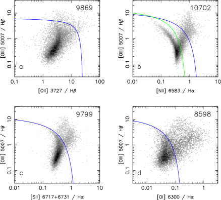
Figure 1: Our sample galaxies in four classical emission line ratio diagnostic diagram: [O iii]/H$\beta$ vs [O ii]/H$\beta$ (a), [O iii]/H$\beta$ vs [N ii]/H$\alpha$ (b), [O iii]/H$\beta$ vs [S ii]/H$\alpha$ (c) , [O iii]/H$\beta$ vs [O i]/H$\alpha$  (d). The grey scale level represents the number of galaxies in each pixel, darker pixels being more populated. The total number of galaxies in the various plots is indicated in the top right of each panel. In panel $a$, the line (blue in the on-line version of the paper) represents the empirical curve of Lamareille et al. (2004). In panel $b$, $c$, and $d$ the blue lines represent the Kewley et al. (2001) lines. The green line in panel $b$ represents the Kauffmann et al. (2003) line

.

3 Classical emission line diagrams

Figure 1 shows four classical diagnostic diagrams used to distinguish NSF galaxies from galaxies containing an active nucleus. These are diagrams based on line intensity ratios. Three of them have been popularized by Veilleux & Osterbrock (1987) and have been widely used since then: [O iii]/H$\beta$ vs [N ii]/H$\alpha$ (panel b), [O iii]/H$\beta$ vs [S ii]/H$\alpha$ (panel c), and [O iii]/H$\beta$ vs [O i]/H$\alpha$ (panel d). The fourth one, [O iii]/H$\beta$ vs [O ii]/H$\beta$ (panel a), has been used e.g. by Tresse et al. (1995) or Lamareille et al. (2004). The [O iii]/H$\beta$ vs [N ii]/H$\alpha$ has actually been introduced by Baldwin et al. (1981), and will be referred to as the BPT diagram. The total number of galaxies in each diagram is indicated in the plots. In order to do these plots, we have imposed no condition on the signal-to-noise in the line, thus an object appears here as soon as we are able to measure the intensities of all the emission lines involved in the plot. Thus, about half of the galaxies of our initial sample have at least four relevant emission lines detected and are represented in this diagram. The rest of the galaxies have either between 1 and 3 of those lines detected, or none of them. Galaxies of this latter group are called passive galaxies. Note that restricting the diagrams of Fig. 1 only to objects with a signal-to-noise ratio of at least 3 in each relevant line does not change the apparent distribution of points in the plots, but reduces the proportion of objects in the right wing and in the “body” of the seagull.

The basic idea underlying these diagrams is that the emission lines in NSF galaxies are powered by massive stars, so that there is a well defined upper limit on the intensities of collisionally excited lines with respect to recombination lines (such as H$\alpha$ or H$\beta$). In contrast, AGNs are powered by a source of much more energetic photons so that, globally, collisionally excited lines are more intense, implying that galaxies hosting AGNs should be found to the upper right of NSF galaxies in these diagrams. It has long been known that giant HII regions actually form a very narrow sequence in these diagrams (see eg. Mc Call et al. 1985). This implies that, while a priori the emission line ratios of giant HII regions are defined by three main parameters (namely the metallicity, the mean effective temperature of the ionizing stars and the ionization parameter), these three parameters must be linked together and one may say that the observed sequence is essentially driven by metallicity. The physical reason behind the HII region sequence is not yet clear, but this is an observational fact. Recent spectroscopic surveys of galaxies (e.g. Jansen et al. 2000, Moustakas & Kennicutt 2006) have shown that the emission line sequence of NSF galaxies is actually very close to the giant HII region sequence. The SDSS, with its thousands of galaxies, shows a superb, very narrow sequence in the BPT diagram (the extension to the upper left is very faint in Fig. 1b, because only a small fraction of our sample populates this region of the diagram, which corresponds to very low metallicity star forming galaxies).

The big surprise, with the SDSS, was the apparition of a second sequence, starting from the bottom of the HII region sequence and extending to the upper right of the diagram. This sequence is fuzzier than the HII region sequence, but nonetheless clearly present. Thus, this suggests that line emission in AGN galaxies is shaped by one dominant parameter or by a set of correlated parameters. As a matter of fact, this trend was already suggested in the sample of 285 warm IRAS galaxies studied by Kewley et al. (2001), but it became conspicuous only with SDSS data. Interestingly, the sequence of AGN host galaxies (the right wing of the seagull) appears clearly only in the [O iii]/H$\beta$ vs [N ii]/H$\alpha$ diagram. As seen in Fig. 1, it is very “fuzzy” and forms a small angle with the HII region sequence in the [O iii]/H$\beta$ vs [S ii]/H$\alpha$ and [O iii]/H$\beta$ vs [O i]/H$\alpha$ diagrams and almost merges with the HII region sequence in the [O iii]/H$\beta$ vs [O ii]/H$\beta$ diagram.

The existence of this right wing is obviously of extreme importance for our understanding of the AGN phenomenon. It has been analyzed empirically by Kauffmann et al. (2003) and shown to be linked to the [O iii] luminosity and to the mass of the parent galaxy.

4 Normal star forming galaxies: the left wing of the seagull

4.1 Preliminaries

In studies dealing with statistics of the AGN phenomenon, it is important to have a clear criterion to detect the presence of an AGN. Dopita et al. (2000) and Kewley et al. (2001) have constructed an extensive grid of photoionization models for giant HII regions powered by star clusters. The ionizing radiation field is provided by stellar synthesis models assuming two limiting cases: a constant star formation rate and an instantaneous starburst. They have used different population synthesis codes (PEGASE 2: Fioc & Rocca Volmerange 1997 and Starburst99: Leitherer et al. 1999) and with each code experimented all the available stellar evolutionary track and atmosphere sets. The models were defined by two parameters: the metallicity and the ionization parameter. Kewley et al. (2001) used the entire set of models to define an upper envelope in the diagnostic diagrams of regions that can be powered only by HII regions. As noted by Kauffmann et al. (2003), this upper envelope – the “Kewley et al. line” – is actually well above the NSF sequence delineated by SDSS galaxies.

Two comments are in order. One is that the models of Dopita et al. (2000) were built just before the latest model atmospheres for massive stars (Pauldrach et al. 2001 and Hillier & Miller 1998) were incorporated in public stellar population synthesis codes. These models, which include the effect of non-LTE, mass loss and line blanketing, have a softer radiation field at high metallicity than previous models. Second, there is a priori no reason why the upper envelope should correspond to the observed NSF galaxy sequence. This last argument prompted Kauffmann et al. (2003) to draw an empirical curve separating NSF galaxies from AGN hosts in the [O iii]/H$\beta$ vs [N ii]/H$\alpha$ diagram. It is not quite clear from their paper how they defined this curve, and it too lies slightly above the NSF galaxy sequence (especially in the upper left of the diagram). In any case, it is by extrapolation that they defined the curve in the zone of low values of [O iii]/H$\beta$, where the two wings of the seagull come into contact with its body.

The [O iii]/H$\beta$ vs [N ii]/H$\alpha$ diagram is the most commonly used to separate NSF galaxies from AGN hosts (see e.g. Brinchman et al. 2004, Lamareille et al. 2004, Mouhcine et al. 2005, Gu et al. 2006). In this section, we will look for a sequence of models that fits the upper envelope of the NSF galaxy sequence, and see how this sequence translates in the other traditional diagnostic diagrams shown in Fig. 1.

4.2 Our starting photoionization model grid

Taking advantage of the implementation by Smith et al. (2002) of the Pauldrach et al. (2001) and Hillier & Miller (1998) stellar atmospheres into the Starburst99 code of Leitherer et al. (1999), we have run a grid of photoionization models using the spectral energy distribution provided by that code feeded into the photoionization code PHOTO (using the version described in Stasińska 2005). We have used standard constant star formation models, which are the most appropriate for galaxies containing a large number of HII regions of different ages. We adopted a Salpeter IMF and an upper stellar mass limit of 120M_⊙, which is the canonical parameterization for such kinds of studies. We took the Starburst99 option that uses the Geneva tracks with high mass loss. As explained by Vázquez & Leitherer (2005), this is the recommended option when interested in ionizing spectra. The models of our grid are computed for the following metallicities: $Z$ = 0.1, 0.2, 0.3, 0.4, 0.6, 0.8, 1.0, 1.5 and 2.5 Z_⊙. The metallicities are the same for the nebular gas and for the stars. For the stars, we interpolated from the spectral energy distributions at the two bracketing metallicities available in Starburst99. For the nebulae, we considered that the metallicity is defined by the oxygen abundance, taking a solar value of O/H = $4.9\times 10^{-4}$ (Allende Prieto et al. 2001). We adopted the solar He/H ratio of Grevesse & Sauval (1998) for all the models. The abundances of the $\alpha$-elements with respect to oxygen were chosen to follow the laws found empirically by Izotov et al. (2006) for metal-poor emission line galaxies. For the most important elements in our context, we thus have:

$$\log\frac{\rm Ne}{\rm O}=0.088{\rm X}-1.450,$$ (1)

$$\log\frac{\rm S}{\rm O}=-0.026{\rm X}-1.514,$$ (2)

where X = 12 + log O/H. For nitrogen, we also based on the paper by Izotov et al. (2006), using their Fig. 11 to adopt the following law:

$$\log\frac{\rm N}{\rm O}=-1.6{,\,\,\,\,\,\,\,\,\rm for~{}X}<8,$$ (3)

and

$$\log\frac{\rm N}{\rm O}=0.6({\rm X}-8)-1.6{,\,\,\,\,\,\,\,\,\rm for~{}X}>8$$ (4)

Note that these abundance ratios are different from the solar ones as compiled by Lodders (2003). Since we are interested in emission lines in galaxies, it is more natural to use abundance ratios that are indicated by abundance analysis in such galaxies.

The models are computed for thin bubbles with a constant hydrogen density of $n_{H}$ = 100 cm^-3 (note that, within the range of densities typical of the giant HII regions in emission line galaxies, our results are not affected by the choice of $n_{H}$). The models are characterized by an ionization parameter $U$, defined as $U=Q_{H}/(4\pi R^{2}n_{H}c)$, where $Q_{H}$ is the total number of H-ionizing photons emitted per second by the stars, $R$ is the radius of the bubble in cm and $c$ is the speed of light. The chosen values of $U$ are 10^-2, $5\times 10^{-3}$, $2\times 10^{-3}$, 10^-3, $5\times 10^{-4}$, and $2\times 10^{-4}$. For each value of $U$, we compute a sequence with varying abundances, as explained above. This is obviously a very crude way to model the spectrum of a galaxy seen through a 3″ fibre, as it accounts neither for abundance gradients, nor for diffuse emission, nor for the complex structure of realistic HII regions. Still, they provide useful guidelines to interpret the observed data.

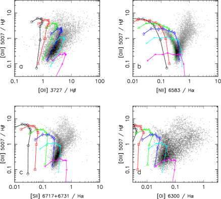
Figure 2: Sequences of photoionization models with varying metallicities $Z$ and constant ionization parameter $U$. The symbols on the curves correspond to the location of models with metallicities $Z$ = 0.1, 0.2, 0.3, 0.4, 0.6, 0.8, 1.0, 1.5 and 2.5 Z_⊙, going from the upper left to the lower right (in panels b, c and d, the lowest metallicity models are actually outside the range of the plots). The values of the ionization parameter $U$ are 10^-2 (black circles), $5\times 10^{-3}$ (red squares), $2\times 10^{-3}$ (green triangles),10^-3 (blue diamonds), $5\times 10^{-4}$ (cyan + signs), $2\times 10^{-4}$ (purple * signs).

These model sequences are shown in Fig. 2. We can see that the upper limit of our sequences lies rather close to the left wing of the seagull in the BPT diagram, especially in the upper part. It is well below the Kewley et al. line (in blue in Fig. 1b, and even below the Kauffmann et al. line (in green in Fig. 1b). As noted in former studies (e.g. Dopita et al. 2000), the observed sequence of star forming galaxies corresponds to only a small selection of a grid sampling a whole range of values of $U$ and $Z$.

Note that the model sequences have slightly different shapes in the various diagrams of Fig. 2. In the [O iii]/H$\beta$ vs [O ii]/H$\beta$ diagram, as the metallicity increases from $Z$ $\simeq$ 0.8 Z_⊙ onwards, models with same $U$ move down and slightly to the left. This is due to the well-known fact that, with increasing cooling, the electron temperature drops, and lines that require a significant amount of energy to be excited, such as [O iii] or [O ii], become weaker. Why then do the sequences of constant $U$ drop rather vertically in the [O iii]/H$\beta$ vs [S ii]/H$\alpha$  and [O iii]/H$\beta$ vs [O i]/H$\alpha$ diagrams? The reason is that the [S ii] and [O i] lines require less energy than [O ii] to be excited, so that the drop in electron temperature is compensated by the increase in element abundance and the intensity of these lines remains roughly constant. Although the [N ii] line has an excitation potential intermediate between that of [O i] and that of [S ii], the lines of constant $U$ in the [O iii]/H$\beta$ vs [N ii]/H$\alpha$  fall down towards the right, i.e. [N ii]/H$\alpha$ increases. This is because, in our models, N/O increases with O/H at large metallicity. It is this different behaviour of the low excitation lines that leads to the different aspects of the observational plots in the various panels of Figs. 1 and 2.

4.3 A sequence of models for the upper envelope of the NSF galaxy sequence

We can use our grid to look for an empirical relation between the ionization parameter and the metallicity that will satisfactorily delineate NSF galaxies in the BPT diagram.

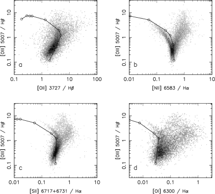
Figure 3: The sequence of photoionization models defined by $\log U=0.916\tanh(-5.42\times Z+3.28)-2.26$ (see Sect. 4.3), and the data from our SDSS sample galaxies, in the four classical diagnostic diagrams.

With the stellar radiation field used in our starting models, we had difficulties in reproducing the tip of the left seagull wing: all the models had slightly too low [O iii]/H$\beta$, meaning that the radiation field is not hard enough. Since the tip of the left wing corresponds to low mass and metallicity galaxies, it is likely that, in most of them, the ionizing radiation field is dominated by that from a recent starburst, as opposed to more massive and metal-rich galaxies which populate the bottom of the left wing, and have a more continuous star-formation regime (Cid Fernandes, Leão & Lacerda 2003). The radiation field from a recent star burst is harder than that provided by stars that are constantly forming at the same rate, because it is dominated by the most massive stars. In models with metallicities lower than 0.7 Z_⊙, we have then replaced the stellar energy distribution resulting from a constant star formation rate with that produced by an instantaneous burst. This improves the modeling of the tip of the left wing, but still does not make it perfect. We have tried other options (changing the geometry, using another stellar synthesis code or another photoionization code), but the problem still remains. As a matter of fact, this problem is not new (Stasińska & Izotov 2003). Whether it requires an additional heating source or a more complex modeling of the HII region to be solved is not yet clear. Anyway, its consequences on the present study are minor, so we set it aside from now on.

We find that the upper envelope of the left wing in the BTP diagram is well reproduced by a sequence of models in which $U$ and $Z$ are related by:

$$\log U=0.916\tanh(-5.42\times Z+3.28)-2.26.$$ (5)

Note that, with our description of the radiation field and with the geometry adopted for the nebular models, there is in principle only one solution for the $U$ – $Z$ relation (however, this relation is ill-determined at low $Z$, as can be understood from Fig. 2b). Other geometries will, of course, lead to slightly different relations.

Fig. 3a–d shows the sequence of models defined by Eq. (5) superimposed on the same observational data as in Fig. 1a–d. We note that the sequence defined by Eq. (5) works also for the [O iii]/H$\beta$ vs.[O ii]/H$\beta$ diagram. On the other hand, the models seem to underpredict the values of [S ii]/H$\alpha$, and even more of [O i]/H$\alpha$. This is not really surprising. It is notorious that simple HII region models produce too small [O i]/H$\alpha$ with respect to observed values in giant HII regions (see e. g. Stasińska & Leitherer 1996). Therefore, we cannot expect, with our schematic models, to reproduce perfectly the line ratios of SDSS galaxies in all the four diagrams at the same time. As shown by Stasińska & Schaerer (1999), explaining [O i] and [S ii]  lines together with the rest of the lines in the spectrum of a giant HII region can be achieved when combining models with different densities. This is feasible when analyzing an individual object, but not tractable in a study like the present one. We have taken the most reasonable option, i.e. to put emphasis on the [O iii]/H$\beta$ vs.[O ii]/H$\beta$  and [O iii]/H$\beta$ vs.[N ii]/H$\alpha$ diagrams.

The results from the model sequence defined by Eq. (5) can be parameterized as follows:

$$\log([\rm{O}\,\textsc{iii}]/{\rm H}\beta)=(0.023606-0.667627Z)\times$$

$$\tanh(-3.412213+5.743451Z)+0.712143$$ (6)

$$\log([\rm{O}\,\textsc{ii}]/{\rm H}\beta)=(-0.86928+0.052482Z)\times$$

$$\tanh(2.66503+4.4425Z)-1.2516$$ (7)

$$\log([\rm{N}\,\textsc{ii}]/{\rm H}\alpha)=(-1.0577-0.055221Z)\times$$

$$\tanh(2.00404-3.82832Z)-1.55079$$ (8)

$$\log([\rm{O}\,\textsc{i}]/{\rm H}\alpha)=(-0.83751+0.110241Z)\times$$

$$\tanh(2.35279-3.97006Z)-2.11304$$ (9)

$$\log([\rm{S}\,\textsc{ii}]/{\rm H}\alpha)=(-0.86928+0.052481Z)\times$$

$$\tanh(2.66503-4.44255Z)-1.251617,$$ (10)

where $Z$ is the model metallicity, with respect to the solar one. Classification boundaries based on these equations are discussed in Sect. 6.1. Note that our series of models for the upper envelope of the NSF galaxy sequence lies much to the left of the Kewley et al. (2001) lines (compare Figs. 3 and 1). The main reason is that Kewley et al. aimed at producing an “extreme theoretical starburst line”, which they obtained using population synthesis models based on Padova evolutionary tracks (Bressan et al. 1993) and stellar atmospheres that were available at that time. As discussed by Vázquez & Leitherer (2005), such population synthesis models strongly overestimate the hardness of the ionizing radiation field. Another point is that, it is only with the SDSS data that the NSF galaxy sequence became conspicuous, and our series of models is meant to model its upper envelope – and not a theoretical upper limit for stellar photoionization.

5 Modeling AGN hosts

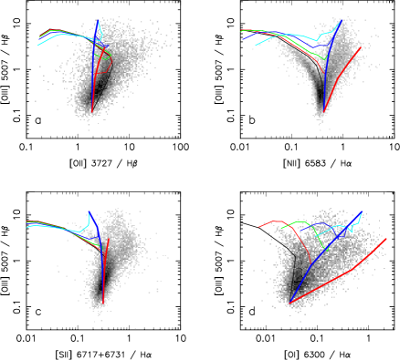
Figure 4: Composite HII regions and AGN models computed by combining the intensities obtained in the HII region sequence represented in Fig. 3 with those of the AGN model sequence with $U$=0.01 (See Sect. 5.1). The thin lines correspond to various proportions $\eta$ between the H$\beta$ luminosity from the AGN and from the HII regions: $\eta$ = 0 (black), 0.03 (red ), 0.1 (green), 0.3 (blue), 1 (cyan). The model metallicities are the same as in Fig. 2. The thick lines connect the composite models at $Z$ = 2.5 Z_⊙ that have $U$ = 0.01 (blue line) and $U$ = 0.03 (red line).

5.1 Composite models

Let us now turn to AGN hosts. The most common current understanding of narrow-line AGNs is that the emission lines are due to moderate density gas ($10^{3}$ – $10^{5}$ cm^-3) photoionized by a radiation field extending to the keV region. We thus consider a very simple model for an AGN, based on the model of Kraemer & Crenshaw (2000) for the narrow-line region of the Seyfert galaxy NGC 1068, which is a broken power-law. We use a density of $10^{4}$ hydrogen particles per cm³ and the same radiation field as proposed by Kraemer & Crenshaw (2000), and we construct a sequence of photoionization models having a given ionization parameter and the same abundances as the HII region model sequences described above.

Inspired by the shape of the BPT diagram, we produced sequences of composite models for AGN galaxies by adding this AGN model sequence to the HII region sequence defined by Eq. (5). The results are shown in Fig. 4, where we plot composite model sequences corresponding to an ionization parameter $U$ equal 0.01 for the AGN and different values of the ratio $\eta$ between the H$\beta$ luminosity produced by the AGN and the H$\beta$ luminosity produced by the HII regions. The values of $\eta$ used in Fig. 4 are 0.03 (red curve), 0.1 (green), 0.3 (blue), and 1 (cyan). The black line represents the models for the upper envelope of the pure HII region sequence defined by Eq. (5). In order to illustrate how composite models in the right wing depend on the value of $U$ adopted for the AGN, we also draw two thick lines that connect composite models with metallicity $Z=2.5$ Z_⊙ for $U$ = 0.01 (blue line) and $U$ = 0.03 (red line).

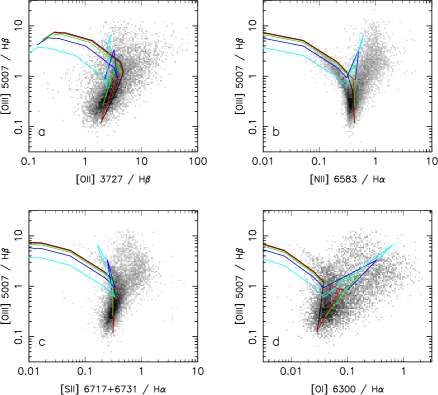
Figure 5: Same as Fig. 4 except that here all the HII region models of various metallicities from the sequence shown in Fig. 3 are now combined with the same AGN model of metallicity $Z$ = 1.5 Z_⊙ (and have $U$ = 0.01)

Fig. 4 shows that such sequences of composite models are very successful – given the simplicity of the approach – in reproducing the observed trends in the observed diagrams. In the BPT diagram, our composite models with $Z$ = 0.6 – 2.5 Z_⊙, the considered range of $\eta$, and a rather small range in $U$ for the AGN (between 0.01 and 0.03) cover the right wing of the seagull quite well. The reason why the composite models do not deviate much from the HII region sequence at low metallicity is clear: it is at high metallicities (solar or higher) that increasing the hardness of the radiation field has the largest effect on collisionally excited lines (see Stasińska 2005 for a discussion of this aspect). Therefore, panel b of Fig. 4 suggests that, even if low metallicity AGN existed, they would not be recognized as such in these emission line ratios diagrams. As far as we are aware, there is at present no hint on the existence of low-metallicity Seyfert nuclei. However, is the AGN phenomenon indeed related to high metallicities or is this belief result of a selection effect?

In Fig. 5, we show the same kind of composite models as in Fig. 4, but this time with the metallicity of the AGN always fixed at 1.5 Z_⊙. We see that composite models with $Z$ $<$ 0.4 Z_⊙ lie rather close to the pure HII region sequence, but this time slightly below it. These models are of course too crude to draw any conclusion on the real effect of a hidden AGN in a metal poor galaxy. On the other hand, at metallicities $Z$ $\geq$ 0.4 Z_⊙, these composite models are in good agreement with the observational diagrams. The [O iii]/H$\beta$ vs [S ii]/H$\alpha$ diagram is the least well reproduced, but by playing a bit more with the parameters (radiation field, gas density in the AGN) should improve the match.

We have thus found a physical and quantitative explanation for the distribution of observational points in the four usual line-ratio diagnostic diagrams. The only thing that we cannot say from these diagrams is whether or not there are AGNs in low metallicity galaxies.

Our models suggest that objects along the right wing differ mainly in the balance between massive stars and AGN ionizing powers (ie., the mixing parameter $\eta$), with the AGN $U$ acting as a second parameter (other AGN-related parameters could come into play as well). Let us compare our sequences of composite models in Fig. 4b with the Kauffmann et al. line and the Kewley et al. line shown in Fig. 1. We find that the Kauffmann et al. line corresponds to composite models in which the AGN contribution to H$\beta$ contribution is no more than 3%. The Kewley et al. line is much less restrictive, and allows for an AGN contribution of roughly 20%.

5.2 The seagull’s wings explained!

One interesting thing to note is that, of the four diagrams presented here, the only one which shows two wide open wings is the [O iii]/H$\beta$ vs [N ii]/H$\alpha$. This is actually a consequence of the fact that, at metallicities larger than about 0.3 Z_⊙, N/O increases with O/H. We know this from observations of galaxies with metallicities between 0.2 and 0.65 Z_⊙  (see e.g. Izotov et al. 2006), where the measurements of the abundances are obtained from direct, empirical methods. For more metal-rich objects, the abundances are generally derived from empirical methods of statistical value, although in a few cases abundances can now be derived by direct methods also (which, in this case, should be examined for possible biases as shown by Stasińska 2005). The observed trends at metallicities above 0.65 Z_⊙(Pilyugin et al. 2003, Bresolin et al. 2005) are clearly of an increase of N/O with O/H. There is a large scatter, though, which can be explained by the enrichment history of the HII regions (see Pilyugin et al. 2003). Therefore, as noted in Sec. 4.2, the HII region sequence falls towards the right in the [O iii]/H$\beta$ vs. [N ii]/H$\alpha$  diagram as metallicity increases, while it falls towards the left in the [O iii]/H$\beta$ vs. [O ii]/H$\beta$ diagram. When an AGN is added, heating of the nuclear region boosts all the optical forbidden lines, which, in the case of the BPT diagram results in the separation of the right wing.

6 Practical ways to distinguish NSF galaxies and AGN host galaxies

With our understanding of the classical diagnostic diagrams as applied to integrated spectra of galaxies, we can now proceed to the main subject of this paper: the classification of galaxies into NSF ones and AGN hosts.

6.1 The boundaries between NSF galaxies and AGN hosts in classical emission line diagrams

It is clear from Fig. 1 that, not only the Kewley et al. line, but also the Kauffmann et al. line are slightly too “generous” in defining the NSF galaxies region. We propose to define pure NSF galaxies those that lie to the left of the curves defined by Eqs. 6 and 8, “hybrid” galaxies those that lie between that curve and the Kauffmann et al. line, and AGN galaxies those that lie to the right of the Kauffmann et al. line. As in the case of the Kauffmann et al. line, there is some degree of subjectivity in defining these boundaries. However, the curve that we propose is closer to the upper envelope of the NSF wing in the [O iii]/H$\beta$ vs [N ii]/H$\alpha$ diagram, and is physically motivated, at least at high values of [O iii]/H$\beta$. The situation is less clearcut on the high metallicity end.

For an easier use, the curve defined by Eqs. (6) and (7) can be approximated by

$$y=(-30.787+1.1358x+0.27297x^{2}){\rm tanh}(5.7409x)$$

$$-31.093,$$ (11)

where $y$= log ([O iii]/H$\beta$), and $x$= log ([N ii]/H$\alpha$). In the following, we will use this expression for the boundary between pure NSF galaxies and galaxies hosting AGNs. This expression is valid for log ([N ii]/H$\alpha$) between -2.0 and -0.4. If [O iii]/H$\beta$ is not measured we consider that a galaxy is an AGN if log [N ii]/H$\alpha$ $>$ -0.4.

As mentioned in Sect. 5.1, the contribution of the AGN to the H$\beta$ emission of galaxies below the Kauffmann et al. line is at most 3%. The zone of the BPT diagram between the curve defined by Eq. (11) and the Kauffmann line is very populated: almost 20% of all the objects appearing in the diagram belong to it. This implies that there is quite a proportion of galaxies that host a very weak AGN in the local Universe.

The [O iii]/H$\beta$ vs [S ii]/H$\alpha$  and [O iii]/H$\beta$ vs [O i]/H$\alpha$ diagrams are obviously less efficient than the BPT one to classify galaxies, both because the dichotomy of the galaxy population is not so clear and because, as shown above, simple photoionization models underpredict the [S ii]/H$\alpha$ and [O i]/H$\alpha$  ratios. In addition, the separation between NSF and AGN galaxies occurs at a value of [O i]/H$\alpha$ where this intensity ratio is difficult to measure.

The [O iii]/H$\beta$ vs [O ii]/H$\beta$ diagram is expected to be even worse than the former two to separate NSF and AGN galaxies. The distribution of the SDSS galaxies in this plane, the fact that [O ii]/H$\beta$ is sensitive to reddening and the behaviour of the model sequences shown in Fig. 2a do not argue in favour of its use. Yet, it has been used, when only blue spectra are available or in the case of redshifted galaxies for which the other diagnostic lines cannot be observed (e.g. Tresse et al. 1995, Lamareille et al. 2004). Using our theoretical borderlines defined by Eq. (12), we find that, in our sample, 4918 objects are classified as NSF galaxies. in the BPT diagram, 6758 are classified as NSF in the [O iii]/H$\beta$ vs [O ii]/H$\beta$ diagram, while only 3504 of those are classified as such in both diagrams. Concerning AGN galaxies, the corresponding counts are 4499, 3853 and 2216 (here, objects for which [O iii]/H$\beta$ could not be measured, were classified as AGN galaxies if [N ii]/H$\alpha$ $>$ 0.4 or if [O ii]/H$\beta$ $>$ 0.5). The comparison between both classification schemes is thus not as bad as it might seem from a mere glance at the observational diagrams. However, it is far from fully satisfactory. Note that, here, we have considered all the galaxies from the initial sample for which the relevant emission lines could be measured, irrespective of the uncertainty in the measured intensities. In a study dealing with the frequency of AGN with respect to other properties of galaxies, one should also discuss the question of the uncertainties in the line ratios, as done for example by Carter et al. (2001).

As demonstrated by Kobulnicky & Phillips (2003), emission lines equivalent widths can be used instead of line intensities to estimate the global metallicities of galaxies. With the same arguments, one can show that equivalent widths ratios can be used in the same way as line intensity ratios to distinguish NSF and AGN galaxies, which is particularly useful in the cases of spectra that are not well calibrated. The same comments as above apply for equivalent widths diagrams.

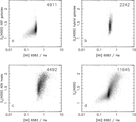
Figure 6: $D_{n}(4000)$ versus [N ii]/H$\alpha$  for NSF galaxies (panel a), hybrid galaxies (panel b), AGN galaxies (panel c) and all our sample galaxies (panel d). The total number of galaxies in the various plots is indicated in the top right of each panel.

6.2 A classification based on [N ii]/H$\alpha$ only?

As a matter of fact, since in the BPT diagram the distribution of the galaxies looks like a flying seagull, one can use the [N ii]/H$\alpha$ ratio alone to classify the galaxies. Of course, the physical interpretation of the [N ii]/H$\alpha$ ratio would be completely different for the two wings. For the left wing, it is a measure of the combination of the metallicity $Z$ and the ionization parameter $U$. Given the strong correlation between both parameters, as evidenced by the fact that the left wing is so thin, [N ii]/H$\alpha$ can then be taken as an empirical measure of the gas metallicity. This has already been mentioned by previous authors for giant HII regions (van Zee et al. 1998, Denicoló, Terlevich & Terlevich 2002, Pettini & Pagel 2004) and can be used for [N ii]/H$\alpha$ up to 0.3–0.4. Larger values of this ratio indicate that the galaxies host an AGN. As [N ii]/H$\alpha$ increases from this value upwards, the effect of the AGN on the galaxy spectra increases and becomes dominant, as can be inferred from Figs. 4b and 5b. However, the right wing of the seagull is rather fuzzy, so that obviously other parameters enter into play and are not correlated. Given our results for the upper limit of the NSF sequence we propose:

$${\rm log}[\rm{N}\,\textsc{ii}]/{\rm H}\alpha\leq-0.4 {\rm NSF},$$

$$-0.4<{\rm log}[\rm{N}\,\textsc{ii}]/{\rm H}\alpha\leq-0.2 {\rm Hybrid},$$

$${\rm log}[\rm{N}\,\textsc{ii}]/{\rm H}\alpha>-0.2 {\rm AGN}$$ (12)

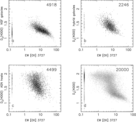
Figure 7: $D_{n}(4000)$ versus EW[O ii] diagram for NSF galaxies (panel a), hybrid galaxies (panel b), AGN galaxies (panel c), and all the sample galaxies (panel d). Galaxies with no measurement of EW[O ii] are plotted at an abscissa of $\sim$ 0.15, and those with no measurement of $D_{n}(4000)$ are plotted at an ordinate of $\sim$ 0.8. The total number of galaxies (including those with artificially assigned values of the abscissa or of the ordinate) in the various plots is indicated in the top right of each panel.

Being able to distinguish between NSF and AGN galaxies using one criterion only is very useful since it allows one to study the effect of any other parameter by a simple 2D-plot. We show an example in Fig. 6, where we plot the 4000 Å break index, $D_{n}(4000)$ , as a function of [N ii]/H$\alpha$ for the NSF galaxies (panel a), the hybrid galaxies (panel b), the AGN galaxies (panel c) and all the galaxies of our sample that can be represented in such a plot (panel d). We see that NSF galaxies tend to have smaller values of $D_{n}(4000)$ than AGN galaxies. There a zone in common, for $D_{n}(4000)$ roughly between 1.2 and 1.5. Still, the dichotomy is important. It indicates that young galaxies are found only among NSF galaxies, while AGN galaxies tend to be old and/or metal-rich. As a matter of fact, as explained in Sect. 5, the BPT diagram does not allow one to distinguish low metallicity AGN galaxies (if they exist) from NSF galaxies, and we already know from our models shown in Sect 5, that objects in the right wing of the seagull are necessarily metal-rich (or rather: have a metal-rich interstellar medium).

This characteristic behaviour of the galaxies in the $D_{n}(4000)$ versus [N ii]/H$\alpha$ diagram suggests that one could perhaps use the stellar properties to distinguish NSF and AGN galaxies. This is done in the next subsection.

6.3 A new diagnostic diagram for galaxies at redshifts up to 1.3

The BPT diagram involves the H$\alpha$ and [N ii] lines, meaning that in a survey like the SDSS, which spans the wavelength range 3800 – 9200 Å, it allows one to classify galaxies only up to a redshift of about $z=0.4$. A diagram involving only [O ii], H$\beta$   and [O iii], which is less efficient in separating AGN from NSF galaxies, as seen in the previous sections, could be used for SDSS galaxies up to redshifts of about 0.8.

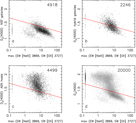
Figure 8: $D_{n}(4000)$ versus max(EW[O ii],EW[Ne iii]) for NSF galaxies (panel a), hybrid galaxies (panel b), AGN galaxies (panel c), and all the sample galaxies (panel d). Galaxies with no measurement of EW[O ii] or EW[Ne iii] are plotted at an abscissa of $\sim$ 0.15, and those with no measurement of $D_{n}(4000)$ are plotted at an ordinate of $\sim$ 0.8. The red line is the adopted boundary between NSF and AGN galaxies, given by Eq. (14).

If we think that an AGN is a hard non-stellar ionizing source with a featureless continuum (Koski 1978), the spectrum of a “pure” AGN galaxy should present emission lines without any sign of the presence of young stars (ages smaller than $10^{7}$ yr). Naturally, young stars can be associated with an AGN, in which case they are often mistaken for a featureless, non-stellar continuum (Cid Fernandes et al 2001, 2004). However, if we could find a way to segregate at least “pure” AGN galaxies using their rest-frame blue spectra, it would be a progress over the present situation, and would allow one extend the classification of galaxies to larger redshifts.

Fig. 6 gives us a clue on how to achieve this goal. The $D_{n}(4000)$ index gives a hint on the stellar population. Large values of $D_{n}(4000)$ indicate the presence of a predominantly old stellar population (Cid Fernandes et al. 2005) and indeed Fig. 6 shows that $D_{n}(4000)$ tends to be large for AGN hosts and small for NSF galaxies (although there is an important overlap). As for the emission lines, their mere presence indicates that ionization is at work (either due to stars or due to an AGN). A commonly used line in the blue is [O ii]. Let us then consider the $D_{n}(4000)$ versus EW[O ii] diagram. We plot it in Fig. 7, in 4 panels, which, as in Figs. 6, correspond to NSF, hybrid, and AGN galaxies as classified by the BPT diagram (panels a, b, and c, respectively) and to our entire sample (panel d). It is clear that NSF and AGN galaxies tend to occupy different zones in the plane. In these figures, we have also represented galaxies with no measurement of EW[O ii]  by plotting them at an abscissa of 0.15, and those with no measurement of $D_{n}(4000)$ (there are only a few ones actually), by plotting them at an ordinate of 0.8.

The [O ii] line may be out of the SDSS spectral range, if the redshift is very small, or it can be in a noisy zone, close to the limit of the observable spectral range. Luckily, the nearby [Ne iii]$\lambda$3869 line provides the same kind of information as [O ii], namely, it indicates the presence of ionized gas. In addition, high excitation AGNs may have a [Ne iii] line much stronger than the [O ii] line, and may be missed if we use only [O ii] to detect them. We therefore merge the information provided by the [O ii]  and [Ne iii]  lines by constructing a diagram similar to Fig. 7, but replacing EW[O ii] by max(EW[O ii],EW[Ne iii]). This diagram (from now on referred to as the $DEW$ diagram) is shown in Fig. 8. As expected, the number of galaxies with the relevant measurements is somewhat larger than in Fig. 7, but the NSF and AGN galaxies continue to occupy different zones with only a small overlap. Guided by Fig. 8d, we define a new borderline between NSF and AGN galaxies by the following equation:

$$D_{n}(4000)=-0.15(\log x+1)+1.7,$$ (13)

where $x$=max(EW[O ii],EW[Ne iii]).

We may now check the correspondence between this new classification into NSF and AGN galaxies, based on the $DEW$ diagram, and the classical one based on the BPT diagram. We find that 4312 galaxies are classified as NSF both in the BPT and in the $DEW$ diagram and 3786 are classified as AGN galaxies in both these diagrams. This is a much better correspondence than between the BPT and the [O iii]/H$\beta$ vs [O ii]/H$\beta$ diagram! We may visualize this correspondence by plotting the galaxies in the BPT diagram for the NSF($DEW$) and AGN($DEW$) galaxies separately (Fig. 9 a and b, respectively). Here, those galaxies without a measurement of [O iii]/H$\beta$ are assigned a value of 0.07 for this ratio, in order to become visible in the plot. We see that this new classification is in quite good agreement with the one based on the BPT diagram using the line defined by Eq. (11). There is a plume of AGN galaxies (according to the BPT diagram) that are classified as NSF according to the $DEW$ criterion (eq. 13). This plume corresponds to the innermost part of the right wing of the seagull, presumably corresponding to higher values of the ionization parameter (as suggested by Fig. 4). A more detailed discussion of this is postponed to a future paper.

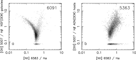
Figure 9: The BPT diagram for NSF(DEW) galaxies (left) and AGN(DEW) galaxies (right). Galaxies without [O iii]/H$\beta$ measured are assigned a value of 0.07 for this ratio. The total number of galaxies in the various plots is indicated in the top right of each panel.

7 Summary

We have considered a sample of 20 000 galaxies extracted from the Sloan Digital Sky Survey and constituting a magnitude-limited sample. We have applied the spectral synthesis technique described in previous papers in this series to the spectra of these galaxies in order to properly subtract the starlight and obtain a pure nebular spectrum. The emission line intensities have been measured with our automated procedure. These data have been used to revisit the classical diagrams that are used to distinguish normal star forming galaxies from galaxies hosting an AGN, and to propose new diagrams.

We first analyzed the four classical emission line ratio diagrams: [O iii]/H$\beta$ vs [O ii]/H$\beta$, [O iii]/H$\beta$ vs [N ii]/H$\alpha$ (the BPT diagram), [O iii]/H$\beta$ vs [S ii]/H$\alpha$, and [O iii]/H$\beta$ vs [O i]/H$\alpha$. From a purely observational point of view, the BPT diagram is the one which best distinguishes two categories of galaxies, as it distributes the galaxies in two wings which look like the wings of a seagull. The left wing, identified with the sequence of normal star forming galaxies, is very narrow. The right wing, which appeared clearly for the first time in the paper by Kauffmann et al. (2003) also based on SDSS galaxies, is constituted of galaxies hosting an AGN. We have computed a series of photoionization models, using as an input the spectral energy distributions from evolutionary stellar population synthesis. We used the population synthesis code Starburst 99 (Leitherer et al. 1999) in the version which incorporates the most elaborated stellar atmospheres for the massive stars (Smith et al. 2002). Our photoionization models confirm this interpretation and allow us to draw physically based divisory lines in all the four classical diagrams. However, the models are too schematic to reproduce the observed [S ii]/H$\alpha$ and [O i]/H$\alpha$ line ratios correctly. Therefore, the model sequence that best divides NSF and AGN galaxies in the [O iii]/H$\beta$ vs [O ii]/H$\beta$ or [O iii]/H$\beta$ vs [N ii]/H$\alpha$  diagrams cannot be safely used to distinguish NSF and AGN galaxies in the [O iii]/H$\beta$ vs [S ii]/H$\alpha$, and [O iii]/H$\beta$ vs [O i]/H$\alpha$ diagrams.

We propose the following divisory line between NSF galaxies and AGN hosts in the BPT diagram:

$$y=(-30.787+1.1358x+0.27297x^{2}){\rm tanh}(5.7409x)$$

$$-31.093,$$ (14)

where $y$= log ([O iii]/H$\beta$), and $x$= log ([N ii]/H$\alpha$), replaced by log ([N ii]/H$\alpha$)=-0.4 if [O iii]/H$\beta$ is not available. This line is actually close to the line drawn empirically by Kauffmann et al. to distinguish NSF galaxies from AGN hosts. We found that the Kauffmann et al. line includes among NSF galaxies objects that have an AGN contribution to H$\beta$ of up to 3%. Thus, depending on the problem one is interested in, one may want to use either the Kauffmann. et al line, or the line we propose in this paper, in order to segregate NSF galaxies from AGN hosts. The Kewley line is much less restrictive, and allows for an AGN contribution of roughly 20%.

Since the BPT diagram is very populated between the line defined by Eq. (11) and the Kauffmann line (it contains about 11% of the galaxies in our sample, including passive galaxies), this means that the local Universe contains a fair proportion of galaxies with very low level nuclear activity, in agreement with the statistics from observations of galactic nuclei eg., Ho, Fillipenko & Sargent (1997).

We point out that emission line ratio diagrams are not efficient in detecting the presence of an AGN in low metallicity galaxies, if such cases exist.

We have shown that a classification into NSF and AGN galaxies using only [N ii]/H$\alpha$  is feasible and useful.

Finally, we propose a new classification diagram (named the $DEW$ diagram), which uses $D_{n}(4000)$ vs max(EW[O ii],EW[Ne iii]). This classification has many advantages:

• It can be used at much larger redshifts than the previous emission line classifications. With SDSS spectra, it can be applied to galaxies with redshifts up to $z=1.3$.

• It requires only a small range in wavelengths, so it can also be used at even larger redshifts in suitable windows in the near infra-red.

• It can be used without a stellar synthesis analysis to subtract the stars.

• It allows one to see all the galaxies in the same diagram, including passive galaxies (the definition of passive assumes a certain detection limit of emission lines). Hence, all galaxies can be classified.

This method has drawbacks too:

• It is not exactly equivalent to the usual BPT classification. But does it matters?

• Old galaxies with a recent starburst ($<10^{7}$ yr) will be mistaken for AGN hosts.

• The borderline between NSF and AGN galaxies is somewhat “porous” (but this is the case of almost any frontier). Note that in the BPT diagram, the borderline is also not very well defined at the low excitation end.

We note that our proposed classification in the $DEW$ diagram is actually more compatible with that based on the [O iii]/H$\beta$ vs [N ii]/H$\alpha$ diagram (when using our boundary line) than a classification based on the [O iii]/H$\beta$ vs [O ii]/H$\beta$ diagram which is used in some papers.

With this new classification scheme at hand, it will be possible to investigate the evolution of AGN galaxy populations in a much larger redshift range than has been done so far, and on firmer grounds.

References

- [\citeauthoryearAbazajian et al.2003] Abazajian K. et al., 2003, AJ, 126, 2081
- [\citeauthoryearAllende Prieto, Lambert, & AsplundAllende Prieto et al.2001] Allende Prieto C., Lambert D. L., Asplund M., 2001, ApJ, 556, L63
- [\citeauthoryearBaldwin, Phillips, & TerlevichBaldwin et al.1981] Baldwin J. A., Phillips M. M., & Terlevich R., 1981, PASP, 93, 5
- [\citeauthoryearBalogh et al.1999] Balogh M. L., Morris S. L., Yee H. K. C., Carlberg R. G., Ellingson E., 1999, ApJ, 527, 54
- [\citeauthoryearBest et al.2005] Best P. N., Kauffmann G., Heckman T. M., Brinchmann J., Charlot S., Ivezić Ž., White S. D. M., 2005, MNRAS, 362, 25
- [\citeauthoryearBresolin et al.2005] Bresolin F., Schaerer D., González Delgado R. M., Stasińska G., 2005, A&A, 441, 981
- [\citeauthoryearBressan et al.1993] Bressan A., Fagotto F., Bertelli G., Chiosi C., 1993, A&AS, 100, 647
- [\citeauthoryearBrinchmann et al.2004] Brinchmann J., Charlot S., White S. D. M., Tremonti C., Kauffmann G., Heckman T., Brinkmann J., 2004, MNRAS, 351, 1151
- [Bruzual A.(1983)] Bruzual A., G. 1983, ApJ, 273, 105
- [\citeauthoryearBruzual & Charlot2003] Bruzual G., Charlot S., 2003, MNRAS, 344, 1000
- [\citeauthoryearCardelli, Clayton, & MathisCardelli et al.1989] Cardelli J. A., Clayton G. C., Mathis J.S., 1989, ApJ, 345, 245
- [\citeauthoryearCarter et al.2001] Carter B. J., Fabricant D. G., Geller M. J., Kurtz M. J., McLean B., 2001, ApJ, 559, 606
- [\citeauthoryearCid Fernandes et al.2001] Cid Fernandes R., Heckman T., Schmitt H., Delgado R. M. G., Storchi-Bergmann T., 2001, ApJ, 558, 81
- [\citeauthoryearCid Fernandes, Leão, & Lacerda2003] Cid Fernandes R., Leão J. R. S., Lacerda R. R., 2003, MNRAS, 340, 29
- [\citeauthoryearCid Fernandes et al.2004] Cid Fernandes R., et al., 2004, ApJ, 605, 105
- [\citeauthoryearCid Fernandes et al.2005] Cid Fernandes R., Mateus A., Sodré L., Stasińska G., Gomes J. M., 2005, MNRAS, 358, 363 (SEAGal I)
- [\citeauthoryearDenicoló, Terlevich, & Terlevich2002] Denicoló G., Terlevich R., Terlevich E., 2002, MNRAS, 330, 69
- [\citeauthoryearDopita et al.2000] Dopita M. A., Kewley L. J., Heisler C. A., Sutherland R. S., 2000, ApJ, 542, 224
- [\citeauthoryearFioc & Rocca-Volmerange1997] Fioc M., Rocca-Volmerange B., 1997, A&A, 326, 950
- [\citeauthoryearFukugita et al.2004] Fukugita M., Nakamura O., Turner E. L., Helmboldt J., Nichol R. C., 2004, ApJ, 601, L127
- [\citeauthoryearGrevesse & Sauval1998] Grevesse N., Sauval A. J., 1998, sce..conf, 161
- [\citeauthoryearGu et al.2006] Gu Q., Melnick J., Fernandes R. C., Kunth D., Terlevich E., Terlevich R., 2006, MNRAS, 366, 480
- [\citeauthoryearHao et al.2005] Hao L., et al., 2005a, AJ, 129, 1795
- [\citeauthoryearHao et al.2005] Hao L., et al., 2005b, AJ, 129, 1783
- [\citeauthoryearHeckman1980] Heckman T. M., 1980, A&A, 87,152
- [\citeauthoryearHeckman et al.2004] Heckman T. M., Kauffmann G., Brinchmann J., Charlot S., Tremonti C., White S. D. M., 2004, ApJ, 613, 109
- [\citeauthoryearHillier & Miller1998] Hillier D. J., Miller D. L., 1998, ApJ, 496, 407
- [Ho et al.(1997)] Ho, L. C., Filippenko, A. V., & Sargent, W. L. W. 1997, ApJS, 112, 315
- [\citeauthoryearHuchra & Burg1992] Huchra J., Burg R., 1992, ApJ, 393, 90
- [\citeauthoryearIzotov et al.2006] Izotov Y. I., Stasińska G., Meynet G., Guseva N. G., Thuan T. X., 2006, A&A, 448, 955
- [\citeauthoryearJansen et al.2000] Jansen R. A., Fabricant D., Franx M., Caldwell N., 2000, ApJS, 126, 331
- [\citeauthoryearKauffmann et al.2003c] Kauffmann G. et al., 2003, MNRAS, 346, 1055
- [\citeauthoryearKauffmann et al.2004] Kauffmann G., White S. D. M., Heckman T. M., Ménard B., Brinchmann J., Charlot S., Tremonti C., Brinkmann J., 2004, MNRAS, 353, 713
- [\citeauthoryearKewley et al.2001] Kewley L. J., Dopita M. A., Sutherland R. S., Heisler C. A., Trevena J., 2001, ApJ, 556, 121
- [\citeauthoryearKewley & Dopita2002] Kewley L. J., Dopita M. A., 2002, ApJS, 142, 35
- [\citeauthoryearKobulnicky & Phillips2003] Kobulnicky H. A., Phillips A. C., 2003, ApJ, 599, 1031
- [\citeauthoryearKoski1978] Koski A. T., 1978, ApJ, 223, 56
- [\citeauthoryearKraemer & Crenshaw2000] Kraemer S. B., Crenshaw D. M., 2000, ApJ, 544, 763
- [\citeauthoryearLamareille et al.2004] Lamareille F., Mouhcine M., Contini T., Lewis I., Maddox S., 2004, MNRAS, 350, 396
- [\citeauthoryearLeitherer et al.1999] Leitherer C., et al., 1999, ApJS, 123, 3
- [\citeauthoryearLodders2003] Lodders K., 2003, ApJ, 591, 1220
- [\citeauthoryear] Mateus A., Sodré L., Cid Fernandes R., Stasińska G., Schoenell, W., Gomes,J. M. 2006, astro-ph/0511578 (SEAGal II)
- [\citeauthoryearMiller et al.2003] Miller C. J., Nichol R. C., Gómez P. L., Hopkins, A. M., Bernardi M., 2003, ApJ, 597, 142
- [\citeauthoryearMouhcine et al.2005] Mouhcine M., Lewis I., Jones B., Lamareille F., Maddox S. J., Contini T., 2005, MNRAS, 362, 1143
- [\citeauthoryear] Moustakas, J., Kennicutt, R., 2006, astro-ph/0511729
- [\citeauthoryearPasquali, Kauffmann, & Heckman2005] Pasquali A., Kauffmann G., Heckman T. M., 2005, MNRAS, 361, 1121
- [\citeauthoryearPauldrach, Hoffmann, & Lennon2001] Pauldrach A. W. A., Hoffmann T. L., Lennon M., 2001, A&A, 375, 161
- [\citeauthoryearPettini & Pagel2004] Pettini M., Pagel B. E. J., 2004, MNRAS, 348, L59
- [\citeauthoryearPilyugin, Thuan, & Vílchez2003] Pilyugin L. S., Thuan T. X., Vílchez J. M., 2003, A&A, 397, 487
- [\citeauthoryearSchlegel, Finkbeiner, & DavisSchlegel et al.1998] Schlegel D. J., Finkbeiner D. P., Davis M., 1998, ApJ, 500, 525
- [\citeauthoryearSmith, Norris, & Crowther2002] Smith L. J., Norris R. P. F., Crowther P. A., 2002, MNRAS, 337, 1309
- [\citeauthoryearStasińska2005] Stasińska G., 2005, A&A, 434, 507
- [\citeauthoryearStasińska & Izotov2003] Stasińska G., Izotov Y., 2003, A&A, 397, 71
- [\citeauthoryearStasinska & Leitherer1996] Stasinska G., Leitherer C., 1996, ApJS, 107, 661
- [\citeauthoryearStasińska & Schaerer1999] Stasińska G., Schaerer D., 1999, A&A, 351, 72
- [\citeauthoryearStorchi-Bergmann, Ho, & Schmitt2004] Storchi-Bergmann T., Ho L. C., Schmitt H. R., 2004, IAUS, 222
- [\citeauthoryearTremonti et al.2004] Tremonti C. A., et al., 2004, ApJ, 613, 898
- [\citeauthoryearTresse et al.1996] Tresse L., Rola C., Hammer F., Stasinska G., Le Fevre O., Lilly S. J., Crampton D., 1996, MNRAS, 281, 847
- [\citeauthoryearvan Zee et al.1998] van Zee L., Salzer J. J., Haynes M. P., O’Donoghue A. A., Balonek T. J., 1998, AJ, 116, 2805
- [\citeauthoryearVázquez & Leitherer2005] Vázquez G. A., Leitherer C., 2005, ApJ, 621, 695
- [\citeauthoryearVeilleux & Osterbrock1987] Veilleux S., Osterbrock D. E., 1987, ApJS, 63, 295
- [\citeauthoryearYork et al.2000] York D. G., et al., 2000, AJ, 120, 1579