FAU-PI1-DISS-06-001

Reconstruction of Neutrino-Induced
Hadronic and Electromagnetic Showers
with the ANTARES Experiment

Den Naturwissenschaftlichen Fakultäten
der Friedrich-Alexander-Universität Erlangen-Nürnberg
zur
Erlangung des Doktorgrades

vorgelegt von
Bettina Diane Hartmann
aus Stuttgart

Zusammenfassung

Die Geschichte der Neutrinophysik begann im Jahr 1930, als Wolfgang Pauli, auf der Suche nach einer Lösung des Rätsels um den Betazerfall, ein leichtes, neutrales Teilchen postulierte. Er nannte dieses Teilchen zunächst Neutron, ehe es dann von Fermi den Namen Neutrino erhielt. Pauli hätte sich wohl damals nicht träumen lassen, dass 75 Jahre später für den Nachweis dieser Teilchen Detektoren mit einem instrumentierten Volumen von bis zu einem Kubikkilometer existieren bzw. sich im Bau befinden würden. Eines dieser riesigen Neutrinoteleskope ist das ANTARES-Experiment [ANT99]. Dieses 0.03 km³ große Neutrinoteleskop wird derzeit vor der Französischen Mittelmeerküste in 2400 m Meerestiefe aufgebaut.
Wie der Name Teleskop bereits andeutet, haben Neutrinoteleskope die Vermessung von aus großen Entfernungen kommenden Signalen zum Ziel, in diesem Fall von Neutrinos, die im Kosmos erzeugt werden. Man geht davon aus, dass die meisten Quellen kosmischer Gamma-Strahlung, wie z.B. Gammastrahlenblitze (engl. Gamma Ray Bursts), Aktive Galaktische Kerne oder Supernova-Überreste, neben Gammastrahlen auch hochenergetische Neutrinos, d.h. Neutrinos mit Energien $>1$ GeV, in großer Zahl produzieren. Neutrinos haben wegen ihres sehr kleinen Wirkungsquerschnittes die vorteilhafte Eigenschaft, nur sehr schwach mit dem interstellaren Medium oder stellarem Staub zu wechselwirken, und können daher praktisch aus beliebig großen kosmischen Entfernungen ohne Abschwächung zu uns auf die Erde gelangen. Der extrem kleine Wirkungsquerschnitt birgt jedoch gleichzeitig auch den großen Nachteil, dass Neutrinos nur mit Hilfe sehr großer Targetmassen nachweisbar sind. Aus diesem Grund benutzen Neutrinoteleskope wie ANTARES natürlich vorkommende große, optisch transparente Volumina, wie z.B. das Meer, als Detektormedium.
Neutrinos können nur indirekt, über ihre Reaktionsprodukte, nachgewiesen werden. Experimente wie ANTARES nutzen für den Nachweis der Reaktionsprodukte den so genannten Cherenkov-Effekt [Che37]: Wenn geladene Teilchen ein Medium mit einer Geschwindigkeit durchfliegen, die größer als die Lichtgeschwindigkeit in diesem Medium ist, emittieren sie entlang ihrer Bahn unter einem festen, vom Brechungsindex des Mediums abhängigen Winkel Photonen. Für Meerwasser liegt dieser Winkel bei ca. 42^∘. Die Cherenkov-Photonen können mit Hilfe von Photomultipliern nachgewiesen werden. Aus den gemessenen Photonensignalen werden dann wiederum die Energie und Richtung des primären Neutrinos rekonstruiert.
Der ANTARES-Detektor wird in seiner endgültigen Form aus 900 Optischen Modulen (OMs) bestehen, die je einen Photomultiplier enthalten, der über ein Verbindungskabel mit der Ausleseelektronik im Lokalen Kontrollmodul (LCM) verbunden ist. Die OMs sind in Stockwerken zu je drei Stück an vertikalen Kabelstrukturen, den so genannten Strings, befestigt. Der gesamte Detektor wird aus 12 solcher Strings bestehen, mit je 25 Stockwerken in einem vertikalen Abstand von 14.5 m. Abbildung 2 zeigt eine künstlerische Darstellung des ANTARES-Detektors [Mon], mit 8 statt der eigentlichen 25 Stockwerke. Ein einzelnes Stockwerk als Detailansicht ist in Abbildung 2 gezeigt.

Abbildung 1: Künstlerische Darstellung des ANTARES-Detektors [Mon]. Statt der eigentlichen 25 sind zur besseren Übersichtlichkeit nur 8 Stockwerke je String gezeigt.

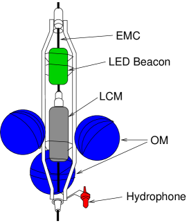
Abbildung 2: Schematische Ansicht eines ANTARES-Stockwerks. Das elektromechanische Verbindungskabel (EMC) ist in schwarz eingezeichnet. Während das Lokale Kontrollmodul (LCM) und die OMs auf allen Stockwerken installiert werden, sind das für die akustische Positionsmessung vorgesehene Hydrophon und der zur optischen Kalibration gedachte LED-Strahler (LED beacon) nur einmal alle fünf Stockwerke vorgesehen.

Die Rekonstruktion der Neutrinorichtung und -energie aus den in den Optischen Modulen gemessenen Signalen gestaltet sich, je nach Ereignisart, unterschiedlich kompliziert. Üblicherweise sind Neutrinoteleskope auf die Rekostruktion von Myon-Ereignissen optimiert, d.h. auf Ereignisse, bei denen das Neutrino unter Austausch des geladenen Stroms mit einem Nukleon aus dem es umgebenden Medium wechselwirkt und ein Myon und einen hadronischen Schauer erzeugt. Da das Myon bei den betrachteten Energien eine sehr viel größere Reichweite als der Schauer hat, ist es in den meisten Fällen das einzige Teilchen, das den Detektor erreicht. Dabei produziert es Cherenkov-Photonen unter einem festen Winkel entlang seiner geraden Spur, sodass die Richtung des Myons, und damit auch die des Neutrinos, auf einige Zehntelgrad genau bestimmt werden können. Ein Nachteil für diese Art von Ereignissen ist jedoch, dass die Energie schwierig zu rekonstruieren ist, da unbekannt ist, welcher Anteil der Myonenspur außerhalb des Detektors verlief.
Das Myon ist jedoch nicht das häufigste Endprodukt in einer Neutrinoreaktion. Dies sind vielmehr die hadronischen Schauer, wobei angemerkt werden muss, dass bei ANTARES aufgrund der im Verhältnis zu den Ausdehnungen eines Schauers groben Instrumentierung nicht zwischen hadronischen und elektromagnetischen Schauern unterschieden werden kann, zumal bei den für diese Studie relevanten Energien im TeV-Bereich und darüber auch der überwiegende Anteil der Teilchen im hadronischen Schauer aus elektromagnetischen Wechselwirkungen stammt. Hadronische Schauer werden sowohl in Neutrinoreaktionen mit geladenem Strom als auch in solchen mit neutralem Strom erzeugt. In letzteren sind sie sogar die einzigen nachweisbaren Bestandteile des Endzustandes, da als weiteres auslaufendes Teilchen ein Neutrino erzeugt wird, welches nicht beobachtet werden kann. Die Rekonstruktion hadronischer Schauer ist daher von großem Interesse, da sie die Untersuchung zusätzlicher Ereignisklassen ermöglicht und somit die durch den kleinen Wirkungsquerschnitt bedingt geringe Ereignisrate erhöht.
Nachteilig auf die Rekonstruierbarkeit von Schauern wirkt sich jedoch deren Richtungs- und Abstrahlcharakteristik aus. Typische Schauerlängen bei den betrachteten Energien zwischen 100 GeV und 100 PeV betragen um die 10 m, was im Verhältnis zu den Abständen der einzelnen Detektorstrings, die zwischen 60 m und 75 m liegen, klein ist. Schauer können somit als quasi punktförmige Ereignisse im Detektor betrachtet werden. Sie werden auch nur dann detektiert, wenn die Neutrinoreaktion im instrumentierten Volumen oder innerhalb eines Bereiches von $\sim 100$ m um den Detektorrand erfolgte, während Myonen noch Kilometer von ihrem Entstehungsort entfernt registriert werden können, wenn sie in Richtung des Detektors fliegen. Die Sensitivität des Detektors ist daher für Schauerereignisse erheblich kleiner als für Myonereignisse. Die kurze Schauerlänge ist auch dafür verantwortlich, dass der Rückschluss vom Schauersignal auf die Neutrinorichtung ungenauer als im Fall des Myons ist. Aufgrund der großen Zahl von Sekundärteilchen im Schauer, die keineswegs alle in Richtung der Schauerachse erzeugt werden, haben die von diesen Sekundärteilchen erzeugten Cherenkov-Photonen verschiedene Winkel in Bezug auf die Schauerachse. Somit entsteht hier auch kein klarer, scharfer Kegel wie beim Myon, sondern eine breite Verteilung, die lediglich ihr Maximum im Bereich des Cherenkov-Winkels von $42^{\circ}$ hat. Abbildung 3 zeigt diese Polarwinkelverteilung für verschiedene Energien in logarithmischer Darstellung, sowie eine im Rahmen dieser Arbeit erstellte Parameterisierung dieser Verteilung.

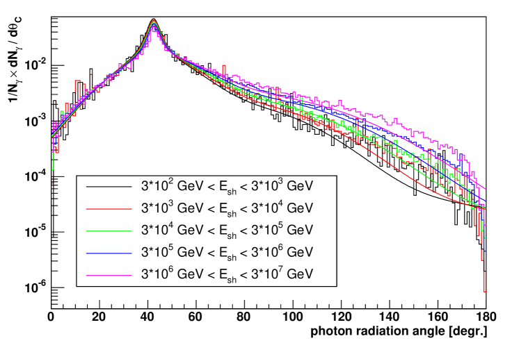
Abbildung 3: Polarwinkelverteilung der Cherenkov-Photonen in Bezug auf die Schauerachse für je eine Dekade in der Schauerenergie, von 300 GeV bis 30 PeV, und die zugehörige Parameterisierungsfunktion, die dem mittleren logarithmischen Energiewert des jeweils betrachteten Energiebereichs entspricht.

Während bei der Richtungsrekonstruktion von Schauern also mit schlechteren Ergebnissen als bei Myonen zu rechnen ist, erwartet man ein deutlich besseres Ergebnis für die Energierekonstruktion des Schauers, da dessen gesamte Energie innerhalb eines verhältnismäßig kleinen Volumens deponiert wird und man von der Annahme ausgehen kann, dass die ausgesandte Lichtmenge proportional zur Energie des Schauers ist. Die Lichtmenge pro Ereignis lässt sich aus den in den Optischen Modulen gemessenen Amplituden berechnen, indem diese auf die Entfernung zum Reaktionsort und die Winkelakzeptanz der Optischen Module in Bezug auf die Photonrichtung korrigiert wurden. Zusätzlich wird die in Abbildung 3 gezeigte Polarwinkelverteilung der Photonen verwendet, um eine Hochrechnung auf die Photondichte des gesamten Raumwinkels vorzunehmen. Da für die genannten Berechnungen die Schauerrichtung benötigt wird, bietet sich eine kombinierte Rekonstruktion von Schauerrichtung und -energie an, wobei beide Größen gleichzeitig variiert werden. Das Auffinden der idealen Werte erfolgt über den Abgleich der für einen momentan angenommenen Wert von Schauerrichtung und -energie erwarteten Amplitude in jedem einzelnen Optischen Modul mit der tatsächlich gemessenen Amplitude. Mit Hilfe eines Log-Likelihood-Fits werden Richtung und Energie dann variiert, bis die maximale Übereinstimmung gefunden ist.
Der Algorithmus erlaubt die Rekonstruktion der Schauerrichtung mit einer Auflösung von $\sim 10^{\circ}$ im Median, für Ereignisse mit einer rekonstruierten Schauerenergie $>5$ TeV. Durch weitere geeignete Schnitte kann der Gesamtwinkelfehler für einzelne Energiebereiche auf Werte bis $2^{\circ}$ reduziert werden, wie aus Abbildung 4 (links) ersichtlich wird. Hier wurde für die jeweils gezeigten Bereiche in der wahren Schauerenergie der Median des Gesamtwinkelfehlers berechnet. Während die Winkelauflösung bis zu einer Schauerenergie von ca. 300 TeV stetig besser wird, steigt sie für noch größere Energien wieder leicht an, was daran liegt, dass dann für die meisten Optischen Module das Sättigungsniveau der Ausleseelektronik erreicht ist.
Zur Darstellung der erzielten Auflösung für die Schauerenergie wird auf der rechten Seite von Abbildung 4 der Logarithmus des Quotienten von rekonstruierter und wahrer Schauerenergie gezeigt. Der Großteil der Ereignisse liegt nahe Null, was einer Übereinstimmung der beiden Werte entspricht. Aus der Standardabweichung von 0.17 ergibt sich, dass die Schauerenergie bis auf einen Faktor $10^{0.17}\approx 1.5$ genau bestimmt werden kann. Dieser Wert wird durch einige Ereignisse bei zu klein rekonstruierten Energien noch verfälscht; die wahre Breite des Maximums, erkennbar durch die an die Verteilung angepasste, in rot eingezeichnete Gaußkurve, liegt bei $\sim 0.14$, was einem Faktor von $1.4$ in der Energie entspricht.

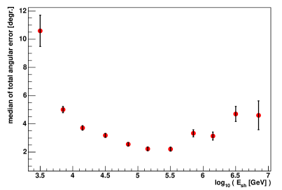
Abbildung 4: Median des Gesamtwinkelfehlers, aufgetragen über der wahren Schauerenergie (links), und Energieauflösung in Bezug auf die Schauerenergie (rechts), für Neutralstromereignisse, nach Schnitten.

Die Effizienz der Schnitte, d.h. der Anteil der den Schnitt passierenden Ereignisse mit gutem Ergebnis (Winkelfehler $<10^{\circ}$), liegt für Schauerenergien oberhalb von 10 TeV bei ca. 70%, wie aus Abbildung 5 (links) ersichtlich wird. In derselben Abbildung rechts ist die Reinheit der Schnitte, d.h. der Anteil der Ereignisse mit gutem Ergebnis (Winkelfehler $<10^{\circ}$) nach den Schnitten an der Gesamtzahl der den Schnitt passierenden Ereignisse, gezeigt. Die Reinheit erreicht einen Wert von ca. 80% zwischen 10 TeV und 1 PeV.

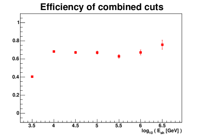
Abbildung 5: Effizienz (links) und Reinheit (rechts) der vorgenommenen Schnitte, aufgetragen über der wahren Schauerenergie.

Bei den gezeigten Ergebnissen handelt es sich um rekonstruierte Neutralstromereignisse. Bei diesem Ereignistyp ist der hadronische Schauer der einzige detektierbare Bestandteil des Endzustandes, und da das Neutrino im Endzustand einen unbekannten Energieanteil trägt, kann für die Primärenergie nur eine untere Grenze in Höhe der Schauerenergie angegeben werden. Anders sieht es bei der Reaktion eines Elektron-Neutrinos über den geladenen Strom aus. Hier geht die gesamte Energie des Primärneutrinos in einen elektromagnetischen und einen hadronischen Schauer über, die mit dem vorliegenden Algorithmus gemeinsam rekonstruiert werden können. Die ermittelte Schauerenergie entspricht dann der Neutrinoenergie, sodass für diesen Ereignistyp nach Schnitten eine Auflösung erzielt werden kann, die einem Faktor 1.4 in der Neutrinoenergie entspricht.
Die hier gezeigten Ergebnisse wurden unter der Annahme einer Sättigung der Elektronik der Photomultiplier bei 200 Photoelektronen (pe) ermittelt. Dieses Sättigungsniveau entspricht der Aufnahme von Wellenformen (WF), welche sehr bandbreiten- und speicherintensiv ist. Die Datennahme in diesem Modus ist mit der Elektronik der Optischen Module zwar möglich, jedoch ist unklar, in wie weit er im fertigen Detektor wirklich genutzt werden wird. Der alternative Aufnahmemodus wäre der so genannte Einzelelektronenmodus (SPE-Modus), bei dem jeweils Amplitude und Zeitpunkt eines Signals aufgezeichnet werden, ohne weitere Informationen über die Wellenform. Dieser Modus verbraucht nur etwa $\frac{1}{40}$ der für Wellenformen benötigten Bandbreite, hat jedoch im Hinblick auf die Schauerrekonstruktion den Nachteil, dass das Sättigungsniveau hier bereits bei etwa 20 pe liegt, und daher der Vergleich zwischen berechneter und gemessener Amplitude bei hohen Energien ungenauer wird. Dies wird in Abbildung 6 deutlich, wo für beide Datennahmemoden der Median des Gesamtwinkelfehlers, vor allen Schnitten, für rekonstruierte Neutralstromereignisse über der Schauerenergie aufgetragen ist.
Die erreichte Auflösung im Bereich bis $\sim 70$ TeV ist für das niedrigere Sättigungsniveau sogar besser als für das höhere, da in diesem Bereich hohe Fluktuation in der Photonenverteilung der einzelnen Ereignissen auftreten können, die durch die niedrigere Sättigung besser unterdrückt werden. Oberhalb von 100 TeV zeigt das niedrigere Sättigungsniveau ein leichte Verschlechterung der Richtungsrekonstruktion um ca. 3^∘ im Vergleich zu einer Sättigung bei 200 pe. Die erreichte Auflösung ist jedoch immer noch gut genug, um eine Richtungsrekonstruktion zu ermöglichen. Zudem zeigt sich in der Energieauflösung kein nennenswerter Unterschied zwischen beiden Moden.

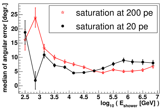
Abbildung 6: Median des Gesamtwinkelfehlers in Abhängigkeit der Schauerenergie, für Sättigung bei 200 pe (WF-Modus, rote Sterne) und bei 20 pe (SPE-Modus, schwarze Kreise), vor allen Schnitten.

Verschiedene Untergrundquellen sind zu berücksichtigen: Zum einen erzeugen radioaktive Zerfälle und Mikroorganismen in der Tiefseeumgebung ein zeitlich und räumlich nur langsam variierendes optisches Rauschen, welches zu unkorrelierten, einzelne Photoelektronen erzeugenden Signalen in den Optischen Modulen führt. Diese Untergrundsignale können durch entsprechend gewählte Kausalitätsbedingungen für die Signalzeitpunkte in verschiedenen Optischen Modulen, sowie die Forderung einer Mindestamplitude, zu großen Teilen unterdrückt werden.
Weitere Untergrundquellen sind atmosphärische Myonen und atmosphärische Neutrinos. Atmosphärische Myonen werden durch die Wechselwirkung kosmischer Wasserstoff- oder anderer Kerne mit der Erdatmosphäre erzeugt und stellen einen gefährlichen, von oben kommenden Untergrund für Schauerereignisse dar, wenn sie nicht eindeutig als Myonen identifiziert werden können. Dies ist dann der Fall, wenn die Myonen durch starke Bremsstrahlungsverluste einen elektromagnetischen Schauer im Detektor induzieren, oder wenn mehrere Myonen gleichzeitig, als so genanntes Myonenbündel, den Detektor passieren. Durch Qualitätsschnitte lassen sich die Myonen, die die Schauerrekonstruktion überlebt haben, zu über 99% unterdrücken. Der durch atmosphärische Myonen erzeugte Untergrund kann zusätzlich reduziert werden, indem nur von unten kommende Ereignisse betrachtet werden.
Atmosphärische Neutrinos werden wie atmosphärische Myonen durch die Wechselwirkung geladener kosmischer Strahlung mit der Erdatmosphäre erzeugt, können jedoch, anders als erstere, auch von unten, durch die Erde hindurch, den Detektor erreichen. Da atmosphärische Neutrinos nicht von kosmischen Neutrinos unterscheidbar sind, kann dieser Untergrund durch einfache Ereignisselektion nicht unterdrückt werden; kosmische Neutrinos können lediglich als Überschuss über dem erwarteten atmosphärischen Neutrinofluss detektiert werden.
Der atmosphärische Myonen-, bzw. Neutrinountergrund dominiert das Signal der kosmischen Neutrinos unterhalb von 20 TeV bzw. 50 TeV. Die Messung eines isotropen diffusen Flusses ist somit nur oberhalb dieser Energien möglich. Für den verbleibenden betrachteten Energiebereich bis ca. 10 PeV werden noch 0.70 atmosphärische Neutrinos pro Jahr erwartet. Nimmt man an, dass tatsächlich während einer einjährigen Messperiode in ANTARES ein einziges Ereignis detektiert worden ist und dass der kosmische Neutrinofluss proportional zu $E_{\nu}^{-2}$ ist, so ergibt sich daraus, mit einem Konfidenzniveau von 90%, eine enegieunabhängige Obergrenze des kosmischen Neutrinoflusses von

$$E_{\nu}^{2}{\Phi_{90\%}}=1.7\times 10^{-7}\,\textrm{GeV cm}^{-2}\,\textrm{s}^{-1}\,\textrm{sr}^{-1}$$

für den betrachteten Energiebereich zwischen 50 TeV und 10 PeV. Dieser Wert ist in Abbildung 7 als durchgezogene rote Linie, im Vergleich zu den für Schauer gemessenen Obergrenzen der Neutrinoexperimente AMANDA [AMA04a] und BAIKAL [Wis05], sowie zu den bei MACRO gemessenen [MAC03], bzw. für ANTARES berechneten [Zor04] (graue Linien) Obergrenzen für Myon-Ereignisse, gezeigt. Die in grün gezeigten atmosphärischen Neutrinoflüsse entsprechen dem Modell von Bartol [Agr96] für verschiedene Einfallwinkel. Die weiteren Eintragungen zeigen verschiedene theoretische Obergrenzen des Neutrinoflusses nach Modellen von Waxman und Bahcall [Bah99, Bah01] (blaue, mit WB und max. extra-galactic p beschriftete Linien; Mannheim, Protheroe und Rachen [Man00] (türkisfarbene, mit MPR beschriftete Kurven); sowie „top-down”-Modelle [Sig98] (violette, mit TD beschriftete Linien).
Betrachtet man nur von unten kommende Ereignisse, so dominiert oberhalb von $\sim 5$ TeV die Neutrinorate über der Rate fälschlicherweise als von unten kommend rekonstruierter atmosphärischer Myonen. Der kosmische Neutrinofluss übersteigt den atmosphärischen bei 50 TeV, und oberhalb dieser Energie ist die erwartete Untergrundrate noch 0.35 pro Jahr. Die insgesamt pro Jahr erwartete Untergrundrate ist also in etwa mit Null verträglich. Unter der Annahme, dass nach einjähriger Messung in ANTARES kein einziges Ereignis gefunden wurde, ergibt sich die energieunabhängige Obergrenze für den kosmischen Neutrinofluss mit einem Konfidenzniveau von 90% zu

$$E^{2}{\Phi_{90\%}}^{auf}=3.6\times 10^{-7}\,\textrm{GeV cm}^{-2}\,\textrm{s}^{-1}\,\textrm{sr}^{-1}.$$

Dieser Wert ist in Abbildung 7 als gestrichelte rote Linie eingezeichnet.

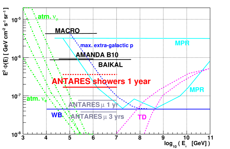
Abbildung 7: Sensitivität für Schauer in ANTARES, die von isotrop einfallenden (durchgezogene rote Linie), bzw. von von unten kommenden Neutrinos (gestrichelte rote Linie) erzeugt wurden, für ein Jahr Messdauer, und im Vergleich dazu Ergebnisse und Erwartungen anderer Ereignisarten und Experimente, welche im Text genauer erläutert werden.

Die vorgelegte Rekonstruktionsstrategie schließt eine große Lücke in der Ereignisrekonstruktion bei ANTARES, da erst durch sie die Rekonstruktion von Ereignissen mit Schauern ermöglicht wird. Damit ist nun prinzipiell die Rekonstruktion aller bei ANTARES auftretenden Ereignistypen möglich. Aufgrund der ohnehin geringen Flüsse der kosmischen Neutrinos ist jede zusätzlich rekonstruierbare Ereignisklasse von großer Bedeutung für die Sensitivität des Experiments.
In einer Weiterentwicklung kann durch die Verbindung dieses Rekonstruktionsalgorithmus mit demjenigen für die Myonrekonstruktion auch eine Verbesserung in der Energierekonstruktion von Myonereignissen erzielt werden, sofern diese so nahe am Detektor stattgefunden haben, dass der hadronische Schauer mit detektiert wurde. In diesem Fall können z.B. die Energien von Myon und Schauer mit den verschiedenen Strategien getrennt rekonstruiert und das Ergebnis dann kombiniert werden.

Contents

1. 1 Introduction
2. 2 Cosmic High-Energy Particles
   1. 2.1 Cosmic Rays: History and Measured Spectrum
      1. 2.1.1 History of Cosmic Ray Detection
      2. 2.1.2 The Cosmic Ray Spectrum
   2. 2.2 Neutrino Physics: Historical Overview
      1. 2.2.1 Postulation of Neutrinos and First Detections
      2. 2.2.2 Solar Neutrinos
      3. 2.2.3 Cosmic Neutrinos
   3. 2.3 Generation of High-Energy Particles in the Cosmos
      1. 2.3.1 Charged Particles
      2. 2.3.2 Generation of Neutral Particles
   4. 2.4 Sources of High-Energy Cosmic Particles
      1. 2.4.1 Supernova Remnants
      2. 2.4.2 Gamma Ray Bursts
      3. 2.4.3 Active Galactic Nuclei
      4. 2.4.4 Microquasars
3. 3 Neutrino Interactions and Detection
   1. 3.1 Neutrino Interactions
      1. 3.1.1 Kinematic Variables of the Interaction
      2. 3.1.2 Interaction Types and Cross Sections
   2. 3.2 Neutrino Detection
      1. 3.2.1 The Cherenkov Effect
      2. 3.2.2 Neutrino Detection Principle
   3. 3.3 Cosmic Neutrino Fluxes
      1. 3.3.1 Effective Volume and Effective Neutrino Area
      2. 3.3.2 Sensitivity Estimates
      3. 3.3.3 Neutrino Flux from Point Sources
      4. 3.3.4 Diffuse Neutrino Flux
4. 4 The ANTARES Experiment
   1. 4.1 Layout of the Experiment
   2. 4.2 The Optical Modules
   3. 4.3 Data Taking in ANTARES
      1. 4.3.1 Data Digitisation and Data-Taking Modes
      2. 4.3.2 The Software Trigger
   4. 4.4 Optical Properties of the ANTARES Site
      1. 4.4.1 Absorption and Scattering
      2. 4.4.2 Refraction Index and Velocity of Light
   5. 4.5 Status of the Experiment
   6. 4.6 Other Experiments
5. 5 Signal Events in ANTARES
   1. 5.1 The Different Event Classes in ANTARES
      1. 5.1.1 Event Classes with a Track
      2. 5.1.2 Event Classes without a Track
      3. 5.1.3 Other Event Classes
      4. 5.1.4 Event Classification
   2. 5.2 Electromagnetic Cascades
      1. 5.2.1 Longitudinal Profile
      2. 5.2.2 Angular Profile
   3. 5.3 Hadronic Cascades
      1. 5.3.1 Longitudinal Profile
      2. 5.3.2 Angular Profile
      3. 5.3.3 Angle Between Neutrino and Hadronic Shower
6. 6 Background
   1. 6.1 Atmospheric Muons
   2. 6.2 Atmospheric Neutrinos
   3. 6.3 Optical Noise in the Deep Sea
   4. 6.4 Suppression of Optical Background
      1. 6.4.1 Filter Conditions for a Signal Hit
      2. 6.4.2 Event-wise Efficiency and Purity
      3. 6.4.3 Hit-wise Efficiency and Purity
7. 7 Reconstruction of Individual Shower Parameters
   1. 7.1 Reconstruction of the Interaction Vertex
      1. 7.1.1 Method
      2. 7.1.2 Calculation of the Centre-of-Gravity of a Shower
      3. 7.1.3 Results for Events without Background
      4. 7.1.4 Results for Events with Optical Background
   2. 7.2 Reconstruction of the Shower Direction
      1. 7.2.1 Method 1: Using the Cherenkov Angle
      2. 7.2.2 Method 2: Amplitude Ratio
   3. 7.3 Energy Reconstruction
8. 8 Combined Reconstruction of Shower Parameters
   1. 8.1 Pattern Matching Algorithm
      1. 8.1.1 Geometrical Situation, OM Efficiency and Attenuation
      2. 8.1.2 Angular Photon Distribution
      3. 8.1.3 Calculation of the Photo-Electron Number from the Hit Amplitudes
      4. 8.1.4 Comparison of the Measured and the Calculated Hit Amplitudes
   2. 8.2 The Maximum Likelihood Fit
      1. 8.2.1 Starting Values for the Fit
      2. 8.2.2 Calculation of Neutrino Energy from the Photo-Electron Number
      3. 8.2.3 Examination of the Likelihood Parameter Space
      4. 8.2.4 Numerical Stability Check
9. 9 Quality Cuts for the Event Selection
   1. 9.1 Suppression of Atmospheric Muons
      1. 9.1.1 Expected and Measured Amplitudes: Quality Cut
      2. 9.1.2 Catastrophic Losses and Multi-Muons in the Remaining Events
   2. 9.2 Comparison of Azimuth from Calculation and Fit
   3. 9.3 Comparison of Energy from Calculation and Fit
   4. 9.4 Large Energies
   5. 9.5 Upgoing Events
   6. 9.6 Cuts Based on Geometrical Considerations
      1. 9.6.1 Events Leaving the Instrumented Volume
      2. 9.6.2 Events Inside the Instrumented Volume
   7. 9.7 Efficiencies and Purities of the Cuts
10. 10 Results of the Reconstruction
    1. 10.1 Reconstruction of NC Events
       1. 10.1.1 Results for SPE Mode
    2. 10.2 Reconstruction of $\nu_{e}$ CC events
    3. 10.3 Effective Volume and Effective Neutrino Area
    4. 10.4 Predictions on Rates and Diffuse Flux Sensitivity
11. 11 Summary and Outlook
12. A ANTARES Event Simulation Packages
    1. A.1 Monte Carlo Event Generation: genhen
    2. A.2 Particle Tracking and Light Generation: geasim
    3. A.3 Hit Selection: Software Filter
    4. A.4 Event Reconstruction: reco
    5. A.5 The Monte Carlo Data Samples
       1. A.5.1 The NC Events
       2. A.5.2 The $\nu_{e}$ CC Events
       3. A.5.3 The Atmospheric Muon Background
13. B Technical Details of the ShowerFitter Package
    1. B.1 Parameters Used for the Reconstruction
    2. B.2 Schematic Description of the Fit
14. C Error Calculations
    1. C.1 Calculation of the Errors on Efficiency and Purity
    2. C.2 Standard Error on the Median

List of Figures

lof

List of Tables

lot

Chapter 1 Introduction

When Wolfgang Pauli postulated the neutrino in 1930, he probably would not have imagined that today, 75 years later, giant instruments for the detection of what he had called a “desperate way out”  of the beta decay puzzle would exist, let alone in such hostile surroundings as the deep sea, or Antarctica. One of these experiments is ANTARES [ANT99], a neutrino telescope that is currently under construction at a depth of 2400 m in the Mediterranean Sea.
The goal of ANTARES is the detection of high-energy neutrinos, i.e. neutrinos with an energy $\gtrsim 50$ GeV, from the cosmos. While neutrinos generated in nuclear power plants and particle accelerators, in the atmosphere of the Earth, and also inside the Sun, have all long been detected in large numbers, the only neutrinos from outside our solar system that have been measured so far are a handful of events from Supernova 1987A [Ale88, Bio87, Hir87] with energies in the 10 MeV range.
Strong evidence exists, however, that high-energy cosmic neutrinos are generated in powerful cosmic particle accelerators, like Supernova Remnants or Gamma Ray Bursts: Air shower experiments on Earth measure high rates of high-energy charged cosmic rays, for which these stellar accelerators are possible sources. As these sources can be associated with dense matter concentrations, it is expected that a part of the accelerated cosmic rays interacts with this dense matter to produce secondary photons and neutrinos. Photons at TeV energies from these sources have already been measured, and astroparticle physicists are therefore convinced that it is only a matter of time until high-energy neutrinos will be detected as well. Theoretical models suggest that the flux of these neutrinos is small, with predicted values around $10^{-6}$ m^-2 s^-1 sr^-1 for energies above 1 TeV. Also, the cross section of neutrinos is very small, because they only interact through the weak force.
The detection efficiency therefore depends crucially on the size of the detector. To enable an experiment to measure a statistically relevant neutrino rate, huge target masses have to be instrumented. This is the reason why neutrino detectors use natural targets like the sea or the Antarctic ice. The transparency of these targets is an important factor for the neutrino detection, because neutrinos can only be detected indirectly, through secondary, charged particles. When travelling faster than the speed of light in the medium, these charged particles produce light, the so called Cherenkov radiation [Che37], which is detected by photomultipliers of the experiment.
Generally, the inelastic neutrino-nucleon interaction cross section exceeds that of the neutrino-electron interaction by several orders of magnitude. When a neutrino interacts inelastically with a nucleon, a hadronic shower and a lepton are produced, the type of the latter depending on the flavour of the incident neutrino ($\nu_{e},\nu_{\mu}$ or $\nu_{\tau}$), and the type of interaction: In charged current reactions, a charged lepton corresponding to the neutrino flavour is produced; in neutral current reactions, the final state lepton equals the incident neutrino. The interaction channels for anti-neutrinos are equivalent, and in the following, if a neutrino channel is mentioned, the respective anti-neutrino channel is always meant as well.
From the detection point of view, the most favourable secondary lepton from a neutrino interaction is the muon, because it can travel over distances up to several km in water, emitting Cherenkov light at a fixed angle along a straight track. This allows for the reconstruction of the muon direction with sub-degree resolution. Therefore, experiments like ANTARES have been optimised for muon detection, and most of the studies conducted so far have specialised on muon reconstruction. This implies, however, the loss of those event classes which are not characterised by an isolated muon track, but instead, by cascades: Hadronic cascades occur in all neutrino-nucleon interactions — in neutral current reactions, the hadronic cascade is even the only detectable part of the interaction; electromagnetic cascades are generated from secondary electrons in the charged current interactions.
This thesis presents the first full and detailed reconstruction strategy inside ANTARES for this class of cascade-, or shower-type events. For the reconstruction of these events, a pattern matching algorithm has been developed. The basic feature of this algorithm is the matching between the amplitudes measured in the photomultipliers of the detector, and their expected values which are calculated assuming a starting value for the energy proportional to the amount of light that is measured in the shower. Under the assumption of a certain position and direction of the shower, and considering the photon directions distributed according to a parameterisation derived from simulations, the expected amplitude for each photomultiplier is calculated. The photon attenuation in water and the angular efficiency of the photomultipliers are taken into account. The matching of the calculated and the measured amplitudes in each photomultiplier is then tested by a likelihood function. Shower direction and energy are varied until the likelihood, and therefore the agreement between expectation and measurement, becomes maximal.
With this algorithm it is possible to reconstruct the direction of a shower in ANTARES with a resolution as good as $2^{\circ}$. The resolution for the reconstruction of the shower energy is usually obtained by fitting a Gaussian to the distribution of ${\log_{10}(E_{reco}/E_{MC})}$. The width $\sigma_{E}$ of the Gaussian describes the logarithmic energy resolution. In this study, a resolution of $\sigma_{E}=0.16$ is reached, which corresponds to a factor of $10^{0.16}\approx 1.4$ in the shower energy. In the case of charged current interactions of electron neutrinos, the shower energy is equivalent to the neutrino energy; for neutral current interactions, the neutrino carries away part of the energy, and the reconstructed shower energy only provides a lower limit on the primary neutrino energy, which introduces an additional bias and error. In comparison, for muon events, resolutions as good as a few tenths of a degree are reached for the reconstruction of the direction, but the muon energy can only be determined within a factor of 2 – 2.5, and provides, as for neutral current events, only a lower limit of the primary neutrino energy.
The content of this thesis is the following: In Chapter 2, a general introduction to the sources and fluxes of cosmic rays is provided, together with a short overview of the history of neutrino physics. Generation mechanisms for high-energy cosmic particles are explained, and a list of the possible or known sources of high-energy neutrinos is given. Chapter 3 illustrates neutrino interactions and the detection of the secondaries and discusses the expected neutrino fluxes. Chapter 4 gives an overview of the ANTARES detector. In Chapter 5, possible event types in ANTARES are presented, and characteristics of electromagnetic and hadronic showers are discussed. In Chapter 6, various background sources, both from atmospheric particles and from optical noise in the deep sea, are described. Different possible algorithms for an individual calculation of the shower position, direction and energy are discussed in Chapter 7. The final strategy for the shower reconstruction is explained in Chapter 8. A set of cuts to separate well reconstructed events from poorly reconstructed ones is described in Chapter 9 which also covers the suppression of atmospheric muon background. The results for different data samples, both neutral current and charged current $\nu_{e}$ events, before and after the cuts, are presented in Chapter 10, together with effective areas and a sensitivity estimate for diffuse neutrino flux. Finally, in Chapter 11, a summary and an outlook to further developments is given.

Chapter 2 Cosmic High-Energy Particles

The cosmic high-energy particles which arrive at Earth can be divided into three classes: Charged particles, denoted cosmic rays for historical reasons, gamma rays, i.e. high-energy photons, and neutrinos.
The detection of cosmic rays, almost 100 years ago, opened the new window of non-optical astronomy and consequently led to the development of stellar acceleration models which predict the generation of high-energy neutrinos. It is therefore appropriate to start this chapter with a short historical introduction on cosmic rays in Section 2.1, together with a description of the measured energy spectrum. Thereafter, a brief overview of the history of neutrino physics follows in Section 2.2. Section 2.3 describes some models for the generation of high-energy particles in the cosmos, while Section 2.4 comments on known and possible sources, with a focus on high-energy neutrinos.

2.1 Cosmic Rays: History and Measured Spectrum

2.1.1 History of Cosmic Ray Detection

The Earth’s exposure to radiation from space was discovered as early as 1912 by the Austrian physicist Victor Hess (1883 - 1964). At that time ionising radiation on Earth had already been detected, but the source of it was still uncertain. It was (correctly) believed that this radiation came from radioactive decays in rocks or other ground matter, and therefore it was expected that with increasing altitudes the radiation would decrease and finally vanish. In an attempt to study this hypothesis, Hess measured the ionisation during several balloon experiments, and found that instead of vanishing, the radiation increased with increasing altitude, which led him to the conclusion that the Earth is exposed to ionising radiation from outside the atmosphere. Hess was awarded the Nobel Prize for this discovery in 1936.
In the decades that followed, cosmic rays were studied mainly with balloon experiments, and later with satellites. However, also ground-based experiments were constructed, the first one by Pierre Auger (1899 - 1993), who discovered extensive air showers, caused by the interaction of high-energy charged primaries with the atmosphere, in 1938. The energy contained in these showers turned out to be several orders of magnitude larger than the energy of the cosmic rays measured with balloons. Starting from 1946, arrays of interconnected detectors to study extended air showers were constructed by groups in the USSR and the USA. It became clear that the cosmic ray flux decreases with increasing energy, according to a power law (cf. Section 2.1.2 and Figure 2.1). Cosmic ray experiments have therefore been built on larger and larger scales, in order to detect particles at highest energies. The largest air shower array to date, the Pierre Auger Observatory [Aug01] which is under construction in Argentina, will cover an area of 3000 km². Its size will allow for the measurement of about 30 cosmic ray events with energies above $10^{20}$ eV a year [Aug01]. The completion of the experiment is expected for mid-2006.

2.1.2 The Cosmic Ray Spectrum

Cosmic rays consist of ionised nuclei, where, for particle energies below some TeV, protons account for the largest fraction, about 90%; helium nuclei make up for about 9% of all cosmic rays, and the rest consists of heavier nuclei up to iron.
The flux of the all-particle spectrum can be described by a power law,

$$\frac{dN}{dE}\propto E^{-\gamma},$$

where $\gamma\approx 2.7$ for energies $\lesssim 4\times 10^{15}$ eV. Figure 2.1 shows the energy spectrum for the all-particle cosmic radiation in an energy range between $10^{6}$ eV and $10^{21}$ eV. Note that the flux shown in this figure was multiplied by $E^{2.5}$, and therefore the spectrum appears less steep. Above about ${4\times 10^{15}}$ eV, the cosmic ray spectrum steepens to $\gamma\approx 3$; because of this change in the slope, the region is referred to as the knee. This effect can be explained phenomenologically by assigning a cut-off energy to the cosmic ray components, proportional to their charge or mass [Hoe04]. This would also explain why at around $4\times 10^{17}$ eV, the slope becomes even steeper, an effect that is called the second knee. This steepening could be caused by the cut-off of heavier elements in the cosmic rays. There are theoretical models [Gai05] which support this explanation by assigning an upper energy limit to some of the cosmic ray sources, so that above a certain energy the proton flux from this source is cut off. Heavier nuclei have larger charges and must therefore be accelerated to larger energies $E$ to achieve the same rigidity $R$ as the protons, ${R=E/(ZeB)}$, where $Ze$ is the charge of the nucleus and $B$ the magnetic field which the nucleus propagates through. Consequently, for heavier elements, the cutoff lies at higher energies. Connected with this suggestion is the assumption that for energies above the knee, heavier nuclei start to dominate over the protons. The exact composition of the cosmic rays at these high energies is very difficult to measure, as experiments on Earth only detect the secondaries of the cosmic rays, after their interaction with the atmosphere. Nevertheless, many important improvements have been achieved during the last years, e.g. by the KASCADE air shower array [KAS03, KAS04].
The cosmic ray spectral index remains stable up to $\sim 10^{19}$ eV. Then the spectrum seems to become harder again, an effect which is called the ankle. A possible explanation [Pet61] for this effect is that an extra-galactic component begins to dominate the spectrum at this energy. However, statistics becomes very small above $10^{19}$ eV, and different experiments are no longer in agreement with each other (see below). From the theoretical point of view, it is expected that protons with an energy of some $10^{19}$ eV start interacting with the Cosmic Microwave Background by formation of $\Delta$-resonances, which would limit their range to $\sim 50$ Mpc. This effect is called the Greisen-Zatsepin-Kuz’min-cutoff (GZK-cutoff) [Gre60, Zat66] and applies to heavier nuclei as well, at the corresponding resonance energies. Additionally, these heavier nuclei lose energy by inducing photo-pair production on the Cosmic Microwave Background. If the GZK-mechanism holds, the sources of the highest-energy cosmic rays measured on Earth must lie within the range of the primary nuclei. As currently no potential source for particles of such high energies is known in the vicinity of our galaxy, a drop in the cosmic ray flux should be observed at the GZK-energy. However, only the measurement of the Fly’s Eye Observatory [Fly99] supports this expectation, whereas the AGASA Experiment [AGA01] observes a flattening of the spectrum, back to smaller values of $\gamma$. The statistics of both experiments are limited; clarification is expected from the new, much larger Pierre Auger Observatory [Aug01] within the next years.

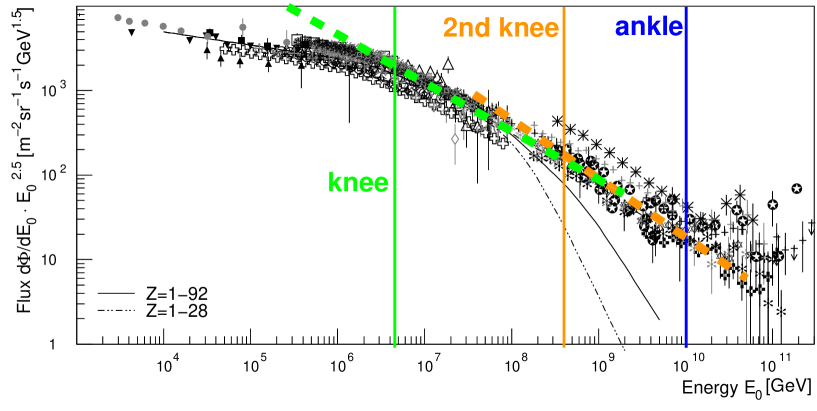
Figure 2.1: All-particle energy spectrum for cosmic rays as measured by different experiments, and according to model calculations (lines marked $Z=1-92$ and $Z=1-28$). Note that the spectrum has been multiplied by $E^{2.5}$. The energies of the knees and the ankle, together with the approximate slope of the distribution, have been marked for better visualisation. After [Hoe05].

2.2 Neutrino Physics: Historical Overview

2.2.1 Postulation of Neutrinos and First Detections

Neutrinos have been postulated by Wolfgang Pauli (1900 - 1958) in 1930 to solve the energy conservation problem in the beta decay of nuclei. In beta decay, the fundamental laws of the conservation of energy, momentum and angular momentum seemed to be violated. Pauli made quite a reckless suggestion to solve the problem, he invented an additional, hitherto unknown particle which would be created in the beta decay and which would carry the missing energy, momentum and spin. This particle would have to be neutral and very light. Pauli suggested to call it neutron; to avoid confusion with the nucleon of the same name, which was discovered two years later (1932) by James Chadwick (1891 - 1974), the name neutrino (“small neutron”) was invented by Enrico Fermi (1901 - 1954). Fermi also formulated a theory for the weak force, based on the neutrino hypothesis.
It took another 14 years, however, until neutrinos, to be more precise, electron anti-neutrinos $\bar{\nu}_{e}$, were finally detected for the first time by Frederick Reines (1918 - 1998) and Clyde L. Cowan, Jr. (1919 - 1974) at the Savannah River Plant. Reines received the Nobel Prize for the detection of the neutrino in 1995. The muon neutrino, $\nu_{\mu}$, was detected only a few years after the electron neutrino, in 1962; it took another 38 years until in 2000 the final direct evidence for the tau neutrino, $\nu_{\tau}$, was found at the Fermilab. Experimental results had indicated before that besides $\nu_{e},\nu_{\mu}$ and $\nu_{\tau}$, no other light neutrinos should exist (here, light means a mass of less than half the mass of the $Z$ boson). The $Z$ boson has been studied extensively at the LEP experiments and its decay width fits very well to the hypothesis of three light neutrino generations [ALE05].

2.2.2 Solar Neutrinos

The dominant nuclear fusion reaction inside the Sun is the $pp$-chain. Neutrinos are produced in this and several other reaction chains at energies ranging from less than 0.1 MeV to 19 MeV. In 1968 the first solar neutrinos were detected by the Homestake experiment [Dav68, Dav94, Hom95]; for a long time they were the only non-terrestrial neutrinos to be measured. A number of large experiments like (Super)Kamiokande [Kos92, SK01] and SNO [SNO00] has been dedicated to the study of solar neutrinos; in 2002, Raymond Davis Jr. (*1914), the initiator of the Homestake experiment, received a Nobel Prize for his studies of the solar neutrinos together with the initiator of the Kamiokande and SuperKamiokande experiments, Masatoshi Koshiba (*1926). Solar neutrino experimentalists were confronted with a big puzzle during long years of thorough studies: The measured flux was significantly smaller than expected from theoretical predictions. Although the surprising solution, neutrino oscillation, was already proposed in the late 1960s [Gri69], the final direct evidence for neutrino oscillations could only be presented in 2001 [SNO02].
Very detailed and precise reviews on solar neutrinos and neutrino oscillations have been written by one of the pioneers of the field, John N. Bahcall (1934 - 2005) [Bah00, Bah04].

2.2.3 Cosmic Neutrinos

Even though neutrinos from the Sun have been studied for several decades, and also detectors for cosmic neutrinos have been planned and built for more than 20 years, cosmic neutrino research is a young and still growing field of studies. An overview of neutrino telescopes is provided in Section 4.6. However, none of these neutrino telescopes has yet been able to identify any cosmic neutrinos. In fact there exists only one proven source of non-terrestrial neutrinos besides the Sun, the Supernova 1987A: On February 23, 1987, around 7:35 UT, the neutrino observatories Kamiokande II, IMB and Baksan have detected a total of 25 neutrinos, with energies in the MeV range, from this Supernova [Hir87, Bio87, Ale88]. The energies and arrival times of the measured signals are shown in Figure 2.2. The experiments had different energy thresholds of 6 MeV (Kamiokande II), 10 MeV (Baksan) and 20 MeV (IMB). There are also uncertainties up to 1 minute in the absolute timing of the experiments; therefore the signals in the plot have been shifted to the same starting point.
Even though the number of detected neutrinos from Supernova 1987A was not large, their detection led to huge activities in the field and a number of new insights, e.g. for the theory of stellar evolution; it was also possible to derive a direct limit of $m_{\nu_{e}}\leq 20$ eV on the electron neutrino mass, from the length of the pulse and the measured neutrino energies [Lon94, p.79].

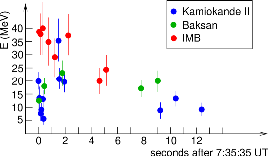
Figure 2.2: Energy and arrival time of the neutrinos from Supernova 1987A [Hir87, Bio87, Ale88]. The signals of the three experiments have been shifted so that they all start at the same time.

2.3 Generation of High-Energy Particles in the Cosmos

2.3.1 Charged Particles

High-energy cosmic rays can be produced either in the “bottom-up” way, by acceleration, or in the “top-down” way, by the decay of super-massive particles. The following explanation of acceleration through the Fermi Mechanism follows the book of Gaisser [Gai90, pp.150-155].

Acceleration: The Fermi Mechanism

The original Second Order Fermi Mechanism, a theory on the acceleration of cosmic rays, was already proposed in the 1940s [Fer49]; it implied, however, the drawback of being too inefficient to allow for an acceleration to high energies. An alternative version of the model was formulated by several authors in the late 1970s [Axf77, Bel78, Bla78, Kry77]: One considers an accumulation of gas through which a shock front moves (caused by a star explosion, for example) with a velocity $\vec{u}$, see Figure 2.3, where the gas is indicated as the light-blue background. The gas in front of the shock is denoted as “upstream” and is considered to be at rest, whereas the shocked gas is denoted “downstream” and has a velocity $-\vec{v}$ relative to the shock front. Therefore, its velocity in the laboratory frame is $\vec{V}=\vec{u}-\vec{v}$. It can be shown that the net energy gain which a particle can receive by moving from upstream to downstream and being reflected by irregularities of the magnetic field in the gas, $\frac{E^{\prime}-E}{E}=\frac{\Delta E}{E}$, is proportional to the relative velocity between shocked and unshocked gas, $\frac{V}{c}=\beta$:

$$\frac{\Delta E}{E}\propto\beta.$$

The acceleration mechanism is therefore called First Order Fermi Mechanism. The particle has to run through the cycle between upstream and downstream gas several 100 times until it is accelerated to TeV energies.
It turns out that the spectral index $\gamma$ for particles accelerated by this mechanism is independent of the absolute magnitude of the gas velocities, but depends instead only on the ratio of the upstream and downstream velocities, and can be approximated as $\gamma\approx 2.1$. The flux at the source should therefore have the same energy dependence for all sources inside which this mechanism holds.
The maximum energy which an accelerated particle can reach through this mechanism depends on the lifetime of the shock front and on the strength of the magnetic fields involved; however, an acceleration to energies above $\sim 100$ TeV – 1 PeV is hard to predict applying the model to the known, mainly galactic, sources.

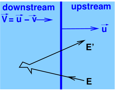
Figure 2.3: Schematic illustration of the First Order Fermi Mechanism: A shock front moves with a velocity $\vec{u}$ through an accumulation of gas; the velocity of the shocked (“downstream”) gas relative to the shock front is $-\vec{v}$. The energy a particle gains when moving from upstream to downstream and being reflected in the magnetic field is proportional to the velocity of the downstream gas in the laboratory frame, $\vec{V}=\vec{u}-\vec{v}$. The cycle between up- and downstream has to be encountered many times for an acceleration to TeV energies. After [Gai90, p.153].

Top-Down Scenarios

A different approach to explain the detection of cosmic particles with energies $>10^{20}$ eV are so called “top-down”  scenarios. In these theories, instead of being accelerated by cosmic objects, the cosmic rays are decay products of super-heavy big-bang relics, which would have masses at the GUT-scale of $10^{24}-10^{25}$ eV. These theories have neither been proven nor disproven, but a fact that seems to contradict them is that one would expect a large number of ultra high-energy gamma rays to be produced in these decays, while studies on the composition of the highest energy cosmic particles conclude that these do not contain of a large fraction of photons [AGA02, Ave02].

2.3.2 Generation of Neutral Particles

Both photons and neutrinos have the advantage compared to cosmic rays that they are electrically neutral and therefore do not undergo deflection in the galactic or extragalactic magnetic fields. Thus, they point back directly to the source where they have been produced.
There are two different mechanism for the production of high-energy gamma rays: Via the decay of neutral pions produced in hadronic interactions, or by electromagnetic interactions, via inverse Compton scattering or bremsstrahlung. Neutrinos, on the other hand, can only be generated in hadronic interactions, and therefore their detection would be a direct proof for hadron acceleration, e.g. according to the Fermi mechanism.

Hadronic Interactions: The Beam Dump Model

The generation of high-energy neutral particles, both neutrinos and photons, in hadronic interactions can be explained by the beam dump model. This model borrows its name from accelerator physics, where the particle beam is “turned off” by deflecting it into a massive target, the beam dump. Hitting the dump, the particles interact with the target matter and produce a large number of secondaries, most of which are absorbed in the dump.
The particles in the cosmic “beam” are the high-energy charged cosmic rays, generated as explained in Section 2.3.1. The cosmic beam dump, and this is the crucial difference to a terrestrial beam dump, consists of a diffuse gas or plasma. Therefore, the range of the mesons produced in the interactions of the “beam” hadrons is long enough to allow them to decay before they are absorbed, yielding neutrinos or photons as decay products.
The most common mesons produced in such a beam dump are charged and neutral pions. The charged $\pi^{\pm}$ produce neutrinos in their decay chains, while the neutral $\pi^{0}$ produces photons (or, to a very small fraction, electrons). The production and decay chains yielding neutrinos (left) and photons (right) are shown in equation (2.1). No distinction has been made here between particles and anti-particles.

$$p+p/\gamma\to \,\pi^{\pm}+ X \hskip 113.81102ptp+p/\gamma\to \pi^{0}+ X$$ (2.1)

$$\hookrightarrow\mu + \nu_{\mu} \hskip 1.42262pt\hookrightarrow\gamma + \gamma$$

$$\hookrightarrow \,e+\nu_{e}+\nu_{\mu}$$

A charged pion decays in 99.99% of all cases into a muon and a muon neutrino; the muon itself decays into an electron, an electron neutrino and another muon neutrino. The $\pi^{0}$ decays in 98.8% of all cases into 2 photons, or else, into an electron-positron pair and a photon.
For the neutrino production chain, it can be seen that for each decaying $\pi$ meson, three neutrinos are produced, with a ratio $\nu_{e}:\nu_{\mu}:\nu_{\tau}=1:2:0$. Due to neutrino oscillations, however, one expects a ratio of $\nu_{e}:\nu_{\mu}:\nu_{\tau}=1:1:1$ on Earth [Ath05].

Electromagnetic Interactions

Contrary to neutrinos, which are only produced in hadronic interactions, high-energy gamma rays can also be generated in electromagnetic interactions: Electrons (and positrons) can be accelerated to very high energies, by the Fermi mechanism described above in Section 2.3.1 or in electromagnetic fields; those electrons produce high-energy gamma rays via bremsstrahlung in the medium that surrounds the source or by inverse Compton scattering, when they transfer a part of their energy to an ambient photon, which then leaves the source as a high-energy gamma ray.
However, the fact that gamma rays interact electromagnetically also limits their range, because they interact with photons in the interstellar medium. The main interaction partners of high-energy gamma rays are photons in the infrared or radio region, and photons from the Cosmic Microwave Background. The latter have a mean energy of the order of $10^{-4}$ eV, so that the cross section for the production of an electron-positron-pair is maximal when the high-energy gamma has an energy of $\sim 10^{15}$ eV. For this energy the mean photon range reaches its minimum of only $\sim 10$ kpc, which is approximately the distance from Earth to the Galactic Centre. Figure 2.4 displays the correlation between the photon range and the photon energy.
Neutrinos, on the other hand, do not interact electromagnetically, and their range is not limited by any interaction partners in the interstellar medium. They could thus be used as messengers even for very distant sources.

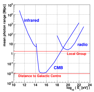
Figure 2.4: Mean photon range over photon energy, and the cosmic interaction partners. As an orientation of the length scale, the distance to the Galactic Centre and the size of the Local Group are shown as well. After [Kou01].

2.4 Sources of High-Energy Cosmic Particles

Generally speaking, all galactic or extragalactic objects where large amounts of energies are released are possible sources of high-energy cosmic particles. The candidate sources listed here have been observed by the photons they emit, which can have all possible wavelengths from radio over visible and X-ray up to wavelengths of $10^{-21}$ m for gamma rays with energies in the range of around 1 PeV, the highest energies which can be measured by ground based gamma ray telescopes using the Imaging Atmospheric Cherenkov Technique, like HESS [HES04]. Gamma rays of even higher energies might have been detected already by air shower experiments, but at these energies, there exists no possibility to clearly identify the type of primary which induced the air shower.
Gamma rays with energies in the GeV range or above cannot be produced any more by thermal processes, they must originate from one of the acceleration mechanisms described above in Section 2.3.2. The sources of such gamma rays are therefore of special interest for neutrino telescopes, as they could be sources for high-energy neutrinos as well, if the acceleration mechanism is of hadronic nature. Recently, the gamma ray experiment HESS has found a TeV gamma ray source with a spectrum favouring a hadronic acceleration process [HES05]. That this is really the case can be proven directly only by measuring neutrinos from the same source.
The most important cosmic accelerators, from the point of view of neutrino detection, are described in the following subsections.

2.4.1 Supernova Remnants

Supernova Remnants are expected to be the main sources of cosmic neutrinos below 1 PeV. A Supernova Remnant is the leftover of a Supernova, the explosion of a massive star at the end of its life. For a short time, the light of this explosion can outshine a whole galaxy. Depending on the mass of the star, the residues of the explosion can either form a neutron star or a black hole. In the common shell-type Supernova Remnants, photons from radio to TeV gamma rays are emitted from an expanding shell. As the recently measured photon energy spectra seem to favour hadronic acceleration processes [HES05], Supernova Remnants are very strong candidates for high-energy neutrinos.
In many cases, a pulsar emerges from a Supernova explosion. Pulsars are stars with a strong magnetic field; they are sources of high-energy gamma rays but the acceleration mechanism is not yet understood. If protons are accelerated inside the magnetic field, neutrinos are produced as well.
It should be mentioned that during the Supernova explosion itself, a large number of neutrinos are produced, but with an energy range of only a few MeV, and thus not detectable for a neutrino telescope like ANTARES.

2.4.2 Gamma Ray Bursts

Gamma Ray Bursts (GRBs) are probably the brightest flashes that exist in the universe. They last only a few seconds and produce an amount of gamma rays which outshines all other gamma sources in the universe for the duration of the explosion.
At present there exist several different GRB models. Some GRBs, but not all, can be associated with an extreme Supernova, a so called Hypernova. A Hypernova is the explosion of a rapidly rotating, very massive star, which collapses into a rapidly rotating black hole surrounded by an accretion disk. Bursts of gamma rays are produced perpendicular to the accretion disc; this is what is detected as the GRB.
GRBs which cannot be associated with a Supernova might be caused by the merging of a binary system of a neutron star and a black hole, two neutron stars or two black holes. This merging would again lead to the formation of a black hole, and an accretion disc with bursts, in the same way as for the Hypernova.
The exact nature and mechanism of the acceleration of particles inside the bursts are still objects of speculations; it is however expected that, associated with the gamma rays, a large amount of neutrinos is produced. If these were detected by a neutrino telescope, a lot of questions on the mechanisms which drive the GRBs could be clarified.

2.4.3 Active Galactic Nuclei

Active Galactic Nuclei (AGN) is the collective term for Seyfert galaxies, radio galaxies, quasars and other high-energy astrophysical objects. These objects have in common that they consist of a galaxy with a super-massive black hole in its centre, and an accretion disc which builds up around the black hole. Highly relativistic jets, which can be up to one Mpc long, are produced perpendicular to the disc. In the special case of one of the jets pointing towards the observer, the AGN is called blazar.
AGNs have been identified as emitters of high-energy gamma rays. If these gamma rays originate from the interactions of accelerated protons in the accretion disc, neutrinos are produced along with them. Production of neutrinos in the jets is expected as well. Theoretical models of AGN are still highly speculative, and therefore the detection of neutrinos from an AGN would be a great step forward in the examination of these objects.

2.4.4 Microquasars

Microquasars are interpreted as galactic binary systems emitting gamma rays in a pattern very similar to that of quasars, but with the scale of emission six orders of magnitude smaller (1 ly, compared to $\sim 10^{6}$ ly for quasars); this is where the name of these objects originates from. Unlike quasars, Microquasars do not consist of a whole galaxy with a black hole or neutron star in its centre, but of a black hole or neutron star of about a solar mass, accompanied by a single star from which it permanently accretes mass. Therefore the relativistic jet which builds up perpendicular to the accretion disc has a much shorter length. Recent calculations [Dis02, Bal03] have shown that Microquasars are very promising candidate sources for high-energy neutrinos. Numbers for the expected neutrino rates of selected Microquasars are provided in Section 3.3.

Chapter 3 Neutrino Interactions and Detection

While the previous chapter was dedicated to the sources and production mechanisms of cosmic neutrinos, this chapter deals with the interactions of neutrinos at (or rather inside) the Earth and the detection of these interactions.
Section 3.1 gives an overview of the possible interactions and the cross sections involved. Section 3.2 explains the principle of a neutrino telescope, and Section 3.3 presents some predictions of neutrino fluxes and equations for the calculation of variables defining the sensitivity of the experiment.

3.1 Neutrino Interactions

Neutrinos are electrically neutral, very light leptons. They interact only through the weak force (and, as all matter, through gravitation). Neutrino cross sections are very small; for example, the $\nu_{\mu}$ on isoscalar nucleon charged current total cross section is $6.77\pm 0.14$ fb/GeV [Eid04]. Therefore, huge target masses are needed for the detection, and the detection can only be indirect, i.e. through the detection of the interaction products.

3.1.1 Kinematic Variables of the Interaction

The reaction of main interest for the neutrino detection in water or other large volumes is the deep inelastic scattering of a neutrino with a target matter nucleon. Figure 3.1 gives a schematic view of the kinematic situation of the interaction.

Figure 3.1: The kinematic situation of the interaction: a neutrino with four-momentum ${p=(E,\vec{p}\,)\approx(|\vec{p}|,\vec{p}\,)}$ interacts with a nucleon with mass $M$ which is at rest before the interaction; the final products are a lepton $l^{\prime}$ and a hadronic shower of momentum $\vec{P}^{\prime}$ and mass $M^{\prime}>M$.

To describe the interaction mathematically, one generally uses the kinematic variables $Q^{2},x$ and $y$. $Q^{2}$ is the negative squared four-momentum transfer between the incoming and the outgoing lepton:

$$Q^{2}:=-(p-p^{\prime})^{2}.$$ (3.1)

For high-energy neutrinos, the interaction partner can be considered to be at rest, so that the rest frame of this particle is equivalent to the laboratory system. For this case, the Bjorken variable $x$ is defined as

$$x:=\frac{Q^{2}}{2M(E-E^{\prime})}\quad.$$ (3.2)

For elastic interactions, $Q^{2}=2M(E-E^{\prime})$, so that $x\equiv 1$. For inelastic reactions, however, $0<x<1$, because in this case ${Q^{2}=2M(E-E^{\prime})+M^{2}-M^{\prime 2}}$. $x$ is therefore a measure for the inelasticity of the interaction [Pov01, p.91]. The hypothetical case of $x\equiv 0$ would be reached if all energy of the neutrino went into the hadronic shower, such that $E^{\prime}=0$. $M^{\prime}$ would then reach its maximum value of ${M^{\prime}=\sqrt{M^{2}+2ME}}$, and $Q^{2}=0$. Therefore, the larger $M^{\prime}$, the smaller $x$. The high-energy neutrino interactions which are subject of this study are deep inelastic, and characterised by $x\ll 1$.
The Bjorken variable $y$ is defined in the laboratory system as

$$y:=\frac{E-E^{\prime}}{E}\quad.$$ (3.3)

$y$ is therefore the relative energy transfer from the neutrino to the hadronic system.

3.1.2 Interaction Types and Cross Sections

Neutrino interactions with matter are to a large extent dominated by the inelastic scattering of the neutrino on a target nucleon, for which the cross section is generally several orders of magnitude larger than for the interaction of a neutrino with an electron. An exception to this, the Glashow resonance, is discussed below.
Neutrinos can interact with a nucleon by exchanging a charged $W^{\pm}$ or a neutral $Z^{0}$ boson. The first interaction type is called Charged-Current interaction, abbreviated CC interaction, while the second type is called Neutral-Current interaction, abbreviated NC interaction. Because of the electro-weak coupling terms which must be taken into account for the neutral current interactions, the NC cross sections are only about one third of the CC cross sections.
There exist several software packages for the calculation of neutrino cross sections which have been compared in detail by [Gan96]. The authors find that the different models agree well up to $\sim 10^{7}$ GeV, while for the highest considered energies of $E_{\nu}=10^{20}$ eV, the uncertainty between the different models is cited as a factor of $2\pm 1$.
The differential cross section for the CC interaction ${\nu_{\mu}+N\to\mu^{-}+anything}$, where $N$ is an isoscalar target nucleon can be expressed in leading order as [Gan96]

$$\frac{d^{2}\sigma}{dxdy}=\frac{2G_{F}^{2}ME_{\nu}}{\pi}\left(\frac{M_{W}^{2}}{Q^{2}+M_{W}^{2}}\right)^{2}[xq(x,Q^{2})+x\bar{q}(x,Q^{2})(1-y)^{2}]$$ (3.4)

where $G_{F}=0.117\cdot 10^{-4}$ GeV^-2 is the Fermi coupling constant (with $\hbar c=1$), $M$ is the mass of the target, $E_{\nu}$ the neutrino energy, $M_{W}$ the mass of the $W$ boson and

$$q(x,Q^{2})=\frac{1}{2}\left(u_{v}(x,Q^{2})+d_{v}(x,Q^{2})\right)+\frac{1}{2}\left(u_{s}(x,Q^{2})+d_{s}(x,Q^{2})\right)$$

$$+s_{s}(x,Q^{2})+b_{s}(x,Q^{2})$$ (3.5)

and

$$\bar{q}(x,Q^{2})= \frac{1}{2}\left(u_{s}(x,Q^{2})+d_{s}(x,Q^{2})\right)+c_{s}(x,Q^{2})+t_{s}(x,Q^{2})$$ (3.6)

are the quark and anti-quark distribution functions, respectively, consisting of the distributions of the valence (indexed $v$) and sea (indexed $s$) quark flavours of the target.
For the NC process ${\nu_{\mu}+N\to\nu_{\mu}+anything}$, the expression for the differential cross section is [Gan96]

$$\frac{d^{2}\sigma}{dxdy}=\frac{G_{F}^{2}ME_{\nu}}{2\pi}\left(\frac{M_{Z}^{2}}{Q^{2}+M_{Z}^{2}}\right)^{2}[xq^{0}(x,Q^{2})+x\bar{q}^{0}(x,Q^{2})(1-y)^{2}]$$ (3.7)

where $M_{Z}$ is the mass of the $Z$ boson, and the NC quark and anti-quark distribution functions are, respectively,

$$q^{0}(x,Q^{2}) =\left(\frac{1}{2}\left(u_{v}(x,Q^{2})+d_{v}(x,Q^{2})\right)+\frac{1}{2}\left(u_{s}(x,Q^{2})+d_{s}(x,Q^{2})\right)\right)\cdot(L_{u}^{2}+L_{d}^{2})$$

$$+\frac{1}{2}\left(u_{s}(x,Q^{2})+d_{s}(x,Q^{2})\right)\cdot(R_{u}^{2}+R_{d}^{2})$$

$$+\left(s_{s}(x,Q^{2})+b_{s}(x,Q^{2})\right)\cdot(L_{d}^{2}+R_{d}^{2})$$

$$+\left(c_{s}(x,Q^{2})+t_{s}(x,Q^{2})\right)\cdot(L_{u}^{2}+R_{u}^{2})$$ (3.8)

and

$$\bar{q}^{0}(x,Q^{2}) =\left(\frac{1}{2}\left(u_{v}(x,Q^{2})+d_{v}(x,Q^{2})\right)+\frac{1}{2}\left(u_{s}(x,Q^{2})+d_{s}(x,Q^{2})\right)\right)\cdot(R_{u}^{2}+R_{d}^{2})$$

$$+\frac{1}{2}\left(u_{s}(x,Q^{2})+d_{s}(x,Q^{2})\right)\cdot(L_{u}^{2}+L_{d}^{2})$$

$$+\left(s_{s}(x,Q^{2})+b_{s}(x,Q^{2})\right)\cdot(L_{d}^{2}+R_{d}^{2})$$

$$+\left(c_{s}(x,Q^{2})+t_{s}(x,Q^{2})\right)\cdot(L_{u}^{2}+R_{u}^{2}).$$ (3.9)

The chiral couplings $L_{u,d}$ and $R_{u,d}$ are defined as

$$L_{u}=1-\frac{4}{3}\sin^{2}\theta_{W},\qquad L_{d}= -1+\frac{2}{3}\sin^{2}\theta_{W}$$

$$R_{u}=-\frac{4}{3}\sin^{2}\theta_{W},\qquad R_{d}= \frac{2}{3}\sin^{2}\theta_{W}$$ (3.10)

where $\sin^{2}\theta_{W}=0.231$ is the weak-mixing angle. From equations (3.4) and (3.7), the total cross sections are determined using standard parton distribution sets like CTEQ6 [Lai95].
For $E_{\nu}>10^{6}$ GeV, the largest contribution to the cross section by far comes from the sea quarks, and the role of the valence quarks becomes small. The limit of $E_{\nu}\to\infty$ corresponds to setting the valence terms in equations (3.1.2),(3.6),(3.1.2) and (3.1.2) to zero; the distribution functions for quarks and anti-quarks are then equivalent, and the cross sections of the anti-neutrino interactions coincide with those of the neutrino interactions.
The total neutrino cross sections are dominated to a very large extent by the deep inelastic scattering reactions of the neutrino on the nucleon. There is, however, one exception: For a $\bar{\nu}_{e}$ with an energy of around 6.3 PeV, the cross section is dominated by the Glashow resonance. At this energy, a $W$ boson is produced resonantly by the CC interaction of the $\bar{\nu}_{e}$ with an electron of one of the target molecules, in the channel $\bar{\nu}_{e}+e^{-}\to W\to anything$.
The cross sections for some selected shower-producing channels ($\nu_{\mu}$ NC, $\bar{\nu}_{\mu}$ NC, $\nu_{e}$ CC and $\bar{\nu}_{e}$ CC) are shown in Figure 3.2. The neutral current interaction of $\nu_{e}$ is expected to be equal to the one of $\nu_{\mu}$.

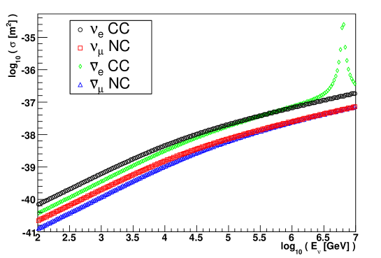
Figure 3.2: Cross sections for neutrino interactions producing showers: neutral current interaction of $\nu_{\mu}$ and $\bar{\nu}_{\mu}$ and charged current interaction of $\nu_{e}$ and $\bar{\nu}_{e}$. The resonance for $\bar{\nu}_{e}$ at 6.3 PeV can be clearly seen. The plot was generated using the values of the CTEQ6 parton distribution functions inside the ANTARES simulation software (see Appendix A.1).

The mean values of $x$ and $y$ are shown in Figure 3.3 as functions of the neutrino energy, for different neutrino interaction types. The values were calculated with the ANTARES simulation software (see Appendix A.1) using the CTEQ6 parton distribution function set [Lai95]. One can see that the mean value of $x$ decreases for higher energies; this poses a challenge to the prediction of neutrino interactions at very high energies, because of the increasing uncertainty of the parton distributions extracted from accelerator experiments. In the case of the Glashow resonance, $x$ is set to zero by the simulation software.
An overview of the interaction products and their characteristics is given in Section 5.1.

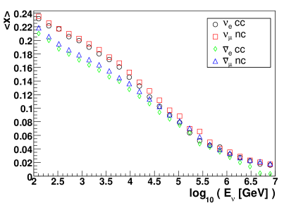
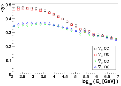
Figure 3.3: Mean values of the Bjorken variables $x$ and $y$ as a function of the neutrino energy. The values were calculated with the ANTARES simulation (see Appendix A.1).

3.2 Neutrino Detection

3.2.1 The Cherenkov Effect

As neutrinos are electrically neutral, they can only be detected by their interaction products. Because of the small neutrino cross sections, neutrino telescopes use a large target mass to register as many neutrino interactions as possible inside, or close to, the detector.
The first generation of neutrino experiments (see Section 2.2), aiming at the detection of low energy neutrinos, used liquid targets of a precisely known chemical composition, and literally counted the number of molecules which had undergone an interaction with a neutrino. A famous example for this type of detector is the Homestake experiment [Hom95].
High-energy neutrino telescopes like ANTARES, AMANDA or others described in Chapter 4, along with other, lower-energy threshold experiments dedicated to the detection of solar and atmospheric neutrinos, like SuperKamiokande [SK01] or SNO [SNO00], are based on a different detection principle. This type of experiment detects the interaction products making use of the Cherenkov effect [Che37]:
When a charged particle moves through a medium, it polarises the atoms along its trajectory, turning them into electric dipoles, as shown symbolically in Figure 3.4a. As long as the particle’s speed $v$ is smaller than the speed of light in the medium, $c/n$ ($n$ being the refraction index of the medium) the dipoles are orientated symmetrically around the particle track, so that the overall dipole moment is zero and no radiation is emitted. However, if the speed of the particle is larger than $c/n$, the symmetry is broken, see Figure 3.4b, and dipole radiation is emitted along the so-called Cherenkov cone. This radiation can be measured in photon detectors.

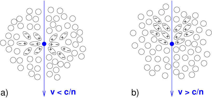
Figure 3.4: a) If the speed $v$ of a charged particle traversing a medium is smaller than the speed of light in the medium, $c/n$, the dipoles induced by polarisation are distributed symmetrically around the particle, and the overall dipole moment is zero. b) If $v>c/n$, the dipole symmetry is broken, and radiation is emitted along the Cherenkov cone. After [Gru93, p.239].

The angle of the Cherenkov cone depends on the refraction index $n$ of the medium and the speed ${v=\beta c}$ of the particle and can be calculated geometrically: During a time $t$, the particle will move a distance $d_{1}=\beta ct$. Light, however, will only move a distance $d_{2}=(c/n)t$. The relation between $d_{1}$ and $d_{2}$ determines the Cherenkov angle $\vartheta_{C}$:

$$\cos\vartheta_{C}=\frac{d_{2}}{d_{1}}=\frac{1}{\beta n}.$$ (3.11)

For reactions of high-energy neutrinos, the interaction products have a velocity $v\approx c$ and thus $\cos\vartheta_{C}\approx 1/n$.

3.2.2 Neutrino Detection Principle

Neutrino telescopes are generally situated deep undersea, underground or under ice, to suppress the high background caused especially by secondary muons from cosmic rays, which produce Cherenkov light in the target material as well. For the ANTARES experiment, the photomultipliers are additionally orientated towards the ground, so that the sensitivity for particles coming from below, which can only be neutrinos, is enhanced. The detection principle is shown schematically in Figure 3.5.

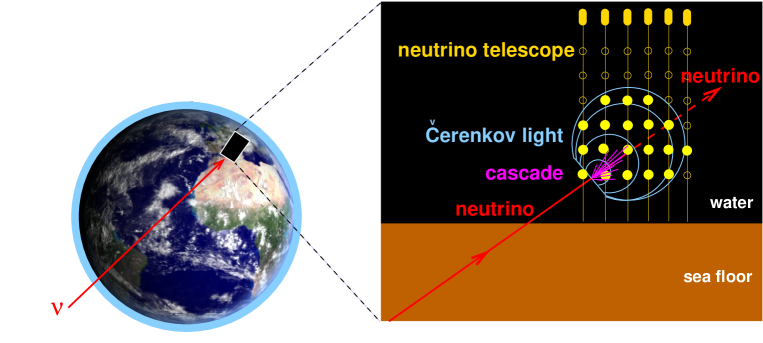
Figure 3.5: Detection principle in a neutrino telescope, shown for the example of a neutral current interaction: The neutrino traverses Earth and interacts somewhere close to the detector. The charged interaction products of the hadronic cascade produce superimposed Cherenkov cones, while the secondary neutrino leaves the detector without producing any signal.

Even though the cross section of neutrino interactions is very small, for neutrino energies above about 1 PeV it becomes large enough to make the Earth opaque for neutrinos. Figure 3.7 shows the interaction length for neutrino-nucleon interactions in terms of km water equivalent, as a function of the neutrino energy. The Earth radius, in the same units, was calculated according to the parameterised Earth density profile [Dzi89] shown in Figure 3.7. One can see that for energies above $\sim 40$ TeV, the neutrino interaction length is smaller than the diameter of the Earth, so that neutrinos with higher energies preferentially enter the detector at larger zenith angles.
Due to the smaller cross section of NC interactions, the corresponding interaction length is larger than the one corresponding to the CC interactions.

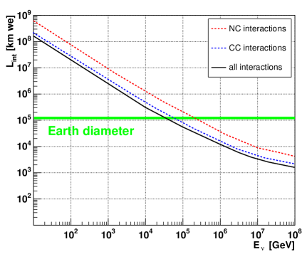
Figure 3.6: Interaction lengths for CC and NC neutrino-nucleon interactions, and total interaction length, given in km water equivalent. The diameter of the Earth, according to the parameterisation in Figure 3.7, is also shown. After [Gan96].

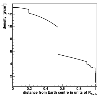
Figure 3.7: Earth density profile, in units of the Earth radius, as parameterised in [Dzi89].

3.3 Cosmic Neutrino Fluxes

In general, one distinguishes between two classes of neutrino fluxes: Diffuse fluxes, i.e. the inseparable superposition of neutrino fluxes from all known or hypothetical sources disregarding their position in space, and fluxes expected from so-called point sources, individual sources of neutrinos which, despite the misleading denomination, may also be extended. Before discussing the two types of fluxes, the variables describing the sensitivity of the experiments are defined.

3.3.1 Effective Volume and Effective Neutrino Area

The effective volume and the effective neutrino area are variables which provide objective measures of the sensitivity of an experiment for a selected reconstruction strategy.
The effective volume $V_{eff}$ is defined as the volume within which the events have been generated, multiplied by the fraction of events that are successfully reconstructed:

$$V_{eff}=V_{gen}\cdot\frac{N_{f}}{N_{gen}}$$ (3.12)

Here, $V_{gen}$ is the generation volume, $N_{gen}$ is the number of events which have been generated inside $V_{gen}$ and $N_{f}$ is the final number of events after the reconstruction or the quality cuts, if any have been applied. The effective volume is generally smaller for shower-type events than for muon-type events, because of the much shorter path length of the showers which limits the interaction volume for detectable event.
The effective neutrino area is the area that a neutrino effectively “sees”  when traversing the instrumented volume. It is calculated by multiplying the effective volume $V_{eff}$ with the number density of molecules in the target matter times the (energy dependent) neutrino interaction cross section and the Earth penetration probability:

$$A_{eff} = \frac{N_{f}}{N_{gen}}\cdot V_{gen} \cdot\rho\cdot N_{A}\cdot\sigma(E)\cdot P_{E}(E,\theta)$$ (3.13)

$$= V_{eff}\quad \cdot\rho\cdot N_{A}\cdot\sigma(E)\cdot P_{E}(E,\theta).$$ (3.14)

In this formula, $\rho$ is the density of the medium inside which the reaction takes place, $N_{A}$ is the Avogadro number (so that $\rho\cdot N_{A}$ is the number of molecules per unit volume in the target), $\sigma(E)$ is the total neutrino-target interaction cross section and $P_{E}(E,\theta)$ is the Earth penetration probability which depends on the zenith angle of the incident neutrino and the neutrino energy, as demonstrated in Figure 3.8 taken from [Lab04]. The Earth absorption was simulated by [Lab04] according to the Earth density profile shown in Figure 3.7 in the previous section.

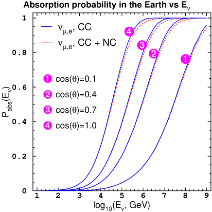
Figure 3.8: Absorption probability for $\nu_{e}$ and $\nu_{\mu}$ when propagating through the Earth, as a function of the incident neutrino energy, for different incident angles. From [Lab04].

3.3.2 Sensitivity Estimates

From the effective neutrino area, the sensitivity for neutrino fluxes from a given source, or for the isotropic diffuse neutrino flux can be predicted. Assuming a flux $\Phi$ which is constant in time and isotropic within the observed angular range, one can calculate the expected number of events $N$ within a given energy range $\{E,E+\Delta E\}$, during the observation period $T$, and within the angular element $\Omega$ as

$$N(E,E+\Delta E)=T\Omega\int_{E}^{E+\Delta E}\Phi(E^{\prime})A_{eff}(E^{\prime})dE^{\prime}.$$ (3.15)

One can invert this equation by assuming that the neutrino flux follows a specific energy spectrum. For cosmic neutrinos, one often assumes that $\Phi(E)=\phi_{0}\cdot E^{-2}$, following the predicted spectrum for the charged particle acceleration in the Fermi mechanism (see Section 2.3.1). The proportionality constant $\phi_{0}$ can then be calculated as

$$\phi_{0}=\frac{N}{T\Omega\int E^{-2}A_{eff}(E)dE}\quad.$$ (3.16)

The sensitivity is then described as the limit on the neutrino flux for a number of events $N$ which is chosen according to the Poissonian statistics for small numbers described in [Fel98]: Depending on the expected background rate, one selects the highest number of events which, at the desired confidence level, is still compatible with the assumption of a background-only detection. The experiment is consequently sensitive to the detection of any neutrino flux causing a higher event rate than the assumed $N$.

3.3.3 Neutrino Flux from Point Sources

A good angular resolution is the crucial factor for the detection of point sources, for two reasons: Firstly, to be able to locate, or even resolve, an individual source as precisely as possible, and secondly, to keep the background as low as possible; as the minimum size of the angular bin increases quadratically with the resolution, so does the rate of background collected within this angular bin. For the ANTARES experiment, theoretical event rates for muons from galactic neutrinos have been estimated for selected source types in [Bal03]. In Figure 3.9 taken from this article, the expected number of events from the two types of sources which are found to be the most promising ones in that article, namely young Supernova Remnants and Microquasars, are shown as examples.
The rates for the young Supernova Remnants were calculated for a theoretical source at 10 kpc distance, 0.1 years after the Supernova explosion. The model used assumes that the whole star has a temperature equal to the surface temperature (“no polar cap heating”); rates for initial pulsar periods of $P_{0}=5$ ms and $P_{0}=10$ ms were calculated. For this theoretical model, the authors arrive at predicted rates of up to 25 detected events per year. For the most promising Microquasar GX339-4, the authors of [Bal03] expect a rate of 6.5 per year.
These predictions seem promising; however, much smaller rates are derived from the measurements of the TeV energy gamma ray experiment HESS [HES04]: For the two strongest TeV gamma ray sources found so far, RXJ0852 and RXJ1317, the detection rates expected for one year of data taking in ANTARES are 0.3 and 0.1 [Kap06], assuming that the neutrino rates at the source are equivalent to the photon rates.
In this context it should also be noted that in a recent study [Hei04] on the potential of detecting point sources in ANTARES using the reaction $\nu_{\mu},\bar{\nu}_{\mu}\to\mu^{\pm}$ it was found that in order to arrive at 50% probability for a $3\sigma$ discovery of an individual source after 2 years of data taking, between 4 (for a source declination of 40^∘) and 8 events (for a source declination of -80^∘) have to be detected from that source.

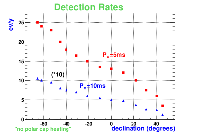
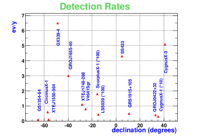
Figure 3.9: Theoretical event rates per year as functions of the absolute source declination in equatorial coordinates, for muons from galactic neutrinos, as calculated for the ANTARES experiment. Left: Event rates from a young Supernova Remnant at 10 kpc distance, for a model with no polar cap heating (see text), and initial pulsar periods of $P_{0}=5$ ms and $P_{0}=10$ ms (the rates for the latter have been multiplied by 10). Right: Event rates for a list of known Microquasars. The rates for ScorpiusX-1 and LS5039 have been multiplied by 100, the rate for CygnusX-1 by 10. From [Bal03].

As the angular resolution for showers is generally poorer than for muon events, the applicability of shower events for point source searches seems doubtful. Exact predictions on the point source sensitivity are beyond the scope of this study and will not be discussed any further. We will only present a very rough estimate on the perspectives, taking into account the following points:

• Angular resolution:
  The angular resolution can be decreased down to $2^{\circ}$ with the help of some quality cuts, as will be shown in Chapter 10. This is still about ten times the angular resolution reached in the reconstruction of muon events. The observational bin would therefore be 100 times larger than for muon events, which means that a priori a correspondingly higher background rate has to be expected. On the other hand, in a study on the expected muon neutrino fluxes from young Supernova Remnants [Pro98], it was found that even if the resolution is only $10^{\circ}$, the muon neutrino flux of a 0.1 year young Supernova Remnant at a distance of 10 kpc, with an initial pulsar period $P_{0}=5$ ms, lies above the atmospheric muon neutrino flux in the ${10^{\circ}\times 10^{\circ}}$ angular bin, for neutrino energies above 10 TeV [Pro98].

• Detectable event classes:
  As will be explained in more detail in Section 5.1, the number of event classes that generate a shower-type event in the detector is larger than the number of event classes which generate a muon event. Taking into account that the cross section for NC interactions is about one third of that of CC interactions (see Section 3.1.2), one can estimate that all 6 NC channels, plus the 2 channels $\nu_{e},\bar{\nu}_{e}+N\to e^{\pm}+X$ produce approximately twice the event rate of the two CC channels $\nu_{\mu},\bar{\nu}_{\mu}+N\to\mu^{\pm}+X$.

• Effective area:
  The effective area tends to be 10 – 15 times smaller for shower events than for muon events. The reason for this is that the much shorter length of the shower (see Figure 5.2 in Section 5.1) leads to a decrease of the effective volume, because only events that are within an absorption length of the instrumented volume can be detected, whereas muons can travel through several km of water towards the detector.

Combining the two latter factors, the sensitivity for shower events deteriorates approximately by a factor of $(2\cdot 0.1)^{-1}=5$. To achieve the same sensitivity as for muons, 5 times more events would be needed; and, taking the first point of the list into account as well, one would expect a 100 times higher background at the same time.
More precise calculations would have to be conducted to retrieve exact predictions on the perspectives of point source searches with shower events in ANTARES; at least from the estimations presented above, the feasibility of such a search seems uncertain.

3.3.4 Diffuse Neutrino Flux

Figure 3.10 shows a collection of theoretical predictions for the diffuse neutrino flux, the superimposed flux of all neutrinos from a certain type of sources. The same plot, with experimental limits added, is shown again at the end of Chapter 4 as Figure 4.15.
The solid blue line marked WB, the upper bound for diffuse neutrino flux calculated by Waxman and Bahcall [Bah99], from now on abbreviated WB bound, is based on the fluxes of cosmic rays measured at Earth at energies from $10^{16}-10^{20}$ eV and on the assumption of a cosmic ray spectrum of $E^{-2}$ at the source, as predicted by the Fermi mechanism, see Section 2.3.1. The predictions are valid for sources which are optically thin for proton photo-meson interactions, in the sense that cosmic rays or photons escape the sources and can be measured at Earth. The WB bound is denoted to be a conservative upper bound by the authors, because it was assumed that the entire energy of the proton is transfered to pions in the photo-meson production, while realistic is a transfer of 20% of the energy. In calculating the upper bound, WB have assumed that only a very small fraction of the cosmic ray flux in the considered energy region is composed of protons and that most of the cosmic ray flux in this energy range comes from heavy nuclei, for which the photo-dissociation cross section is higher than the photo-meson production cross section, so that they cannot account for a large neutrino flux. Assuming that extra-galactic protons yield a higher contribution to the cosmic ray flux than expected, one can exceed the WB bound in the way shown by the dashed blue curve marked “max. extra-galactic $p$” [Bah01], which has however already been partially excluded experimentally, see Figure 4.15 in Section 4.6.
Mannheim, Protheroe and Rachen [Man00] (abbreviated from now on as MPR) do not assume a fixed $E^{-2}$ cosmic ray spectrum at the sources, but take into account source characteristics, like the opacity to neutrons which determines the rate of neutrons which may escape the source. These neutrons would then decay to produce protons which would consequently be measured in the cosmic ray flux. The authors arrive at somewhat higher flux limits, as shown in the cyan coloured lines marked MPR in Figure 3.10. The lower line refers to optically thin sources, i.e. sources that are transparent to neutrons (under the assumption that part of the cosmic rays measured at Earth originate from neutrons that have escaped the source and have then decayed into protons). If one assumes that there exist a lot of optically thick sources, this would mean that the neutrino flux can be much higher than expected from the measured cosmic ray flux because a lot of neutrino sources remain unseen by cosmic ray experiments. The upper, straight line shows the case of optically very thick sources. The actual upper limit on the neutrino flux is expected to be somewhere in between the two lines. Whether the neutrino flux of the lower curve rises again for energies above $10^{9}$ GeV or not depends on the nature of the cosmic rays which have been measured beyond the GZK cutoff. If they are caused by extragalactic sources, their flux is strongly damped by the GZK cutoff, such that the corresponding flux of neutrinos, which do not suffer from attenuation by the GZK mechanism, is expected to be much higher; if, on the other hand, the ultra high-energy cosmic rays are caused by a single strong nearby source, no rise in the neutrino flux is expected; it would stay flat instead, at the limit predicted by WB.
The dashed magenta lines marked TD show the predictions for some top-down models [Sig98]. The limits refer to a model of a GUT particle with an energy of $10^{16}$ GeV, a high universal radio background and a relatively high extra-galactic magnetic field of $10^{-10}$ G. The flux limit marked by the left curve includes supersymmetry, while the right one does not.
The dashed-dotted green curves show the atmospheric neutrino flux, including prompt neutrinos. The two upper lines mark the range of the atmospheric muon neutrino flux, depending on the meson incident angle, while the two lower lines mark the range of the atmospheric electron neutrino flux. The shown flux was simulated inside the ANTARES neutrino interaction simulation (see Appendix A.1); the Bartol model [Agr96] was used to retrieve the conventional flux, and the results of Naumov [Nau01], using the recombination quark-parton model (RQPM) [Bug98], to obtain the prompt neutrino flux. See Section 6.2 for more details on this.

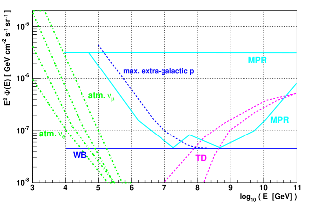
Figure 3.10: Diffuse neutrino fluxes as predicted by different models: Ranges for conventional [Agr96] and prompt atmospheric neutrinos [Nau01]: Green, dashed-dotted lines; Waxman-Bahcall upper limit [Bah99]: Solid blue line marked WB; maximum excess due to extra-galactic protons [Bah01]: Dashed blue line marked max. extra-galactic $p$; Mannheim-Protheroe-Rachen predictions [Man00]: Solid cyan lines marked MPR, upper line for optically thick, lower curve for optically thin sources; top down models [Sig98]: Dashed, magenta lines, with (left) and without (right) SUSY. See text for details.

Chapter 4 The ANTARES Experiment

The ANTARES collaboration was formed in 1996 with the objective to construct and operate a neutrino telescope in the Mediterranean Sea. Currently the collaboration consists of around 150 members from particle physics, astronomy and sea science institutes in 6 European countries. Though the main purpose of the experiment is the detection of high-energy cosmic neutrinos, it is also intended to be used as an experimental platform for studies of the deep-sea environment.
ANTARES is being built in a depth of 2400 m in the Mediterranean Sea, about 40 km South-East of the French coastal city of Toulon. The location of the site is shown in Figure 4.1. As will be discussed in more detail in Chapter 6, the location in the deep sea has the advantage of suppressing to a large extend the background of atmospheric muons produced by cosmic rays. On the other hand, the high water pressure of 240 bar, as well as the aggressive salt water environment, impose strong requirements on the detector components which are designed to have a lifetime of at least 10 years.
A description of the detector components and an overview of the detector layout is given in Section 4.1. The “eyes”  of the detector, i.e. the Optical Modules which actually detect the Cherenkov photons emitted by the charged secondaries produced in neutrino interactions with matter, are described in Section 4.2. The digitisation of the signal is explained in Section 4.3.1. The efficiency of the detector also depends strongly on the optical properties of the environment, i.e. the absorption and scattering length, and the refraction index, all three of them functions of the wavelength. These properties are described in Section 4.4; they are constantly monitored in situ.
During the writing of this thesis, the first out of 12 large detector units (the so-called strings or lines) has been deployed; the completion of the detector is forseen for the year 2007. In Section 4.5, important milestones in the development and construction of the detector are presented, and the current status is reported in more detail.
ANTARES is just one of several experiments aiming at the detection of high-energy cosmic neutrinos. Some of these experiments are already partly or fully operational, others are under construction or in the planning stage. Section 4.6 gives an overview of other neutrino telescopes.

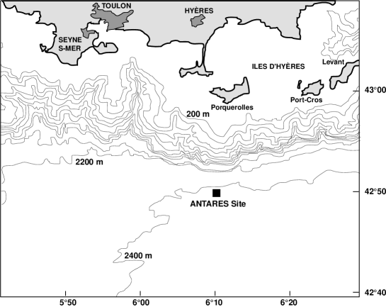
Figure 4.1: Map showing the location of the ANTARES site in the Mediterranean Sea, including the French coast area (in grey) and sea depths. From [ANT99].

4.1 Layout of the Experiment

The ANTARES Optical Modules are mounted on 12 strings, long cables which are fixed to the sea bed by the Bottom String Socket (BSS) and are kept vertically straight by a buoy. The BSS consists of a dead weight, connectors for the cables, an acoustic device to release the string, and the electronics of the String Control Module (SCM). The single elements of the string are both mechanically supported and electrically interconnected by a total of 460 m of Electro-Mechanical Cables (EMC).
One string consists of five sectors, each containing five storeys, so that there are 25 storeys per string. The distance between two storeys is 14.5 m. The unit storey plus corresponding EMC section is called Elementary Segment (ES). Each storey is made up of three Optical Modules (OM) which are supported by the Optical Module Frame (OMF) (see Section 4.2 for a more detailed description of the OMs). The Local Control Module (LCM) is a titanium container placed in the middle of the OMF, housing the data read-out, clock and control electronics for the storey. A schematic view of the string design is given in Figure 4.3, while Figure 4.3 shows an artist’s view of the arrangement of the ANTARES strings [Mon].
Figure 4.4 illustrates the setup of an ANTARES storey in more detail. The figure also shows the hydrophone for the acoustic positioning system and the LED beacon for the time calibration of the photomultipliers. One hydrophone per sector is forseen in each line, and an LED beacon in four of the five sectors of every line. Sound velocimeters required for the acoustic positioning are also planned to be installed on 3 lines. They are not shown in the drawing.
In addition to the 12 detector strings, a 13th string, the Instrumentation Line, is foreseen for the monitoring of environmental parameters. For the first strings, it is planned to use the MILOM, which is already deployed at the ANTARES site, for this task. A more detailed description of the MILOM is given in Section 4.5.
The detector strings are arranged on the sea floor as an octagon, as shown in Figure 4.5. Each string is connected to the Junction Box (JB) by an electro-optical cable. The Junction Box supplies the strings with electrical power and with slow-control and clock signals, and it receives the data taken by the OMs; it contains power converters and the electro-optical interface for data, slow-control and clock transmission. The Junction Box is connected to the shore station located at La Seyne sur Mer by the main electro-optical cable. The shore station houses the control room for the data-taking and the slow-control instruments.

Figure 4.2: Schematic view of an ANTARES string [ANT99]. A full string contains 25 elementary segments (ES). The abbreviations are explained in the text.

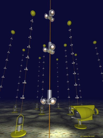
Figure 4.3: Artist’s view [Mon] of the ANTARES detector (not to scale).

Figure 4.4: Schematic view of an ANTARES storey. Mechanical parts are coloured in white, the LCM in grey, the cable in black and the OMs in blue. While the LCM and the OMs are installed on all storeys, the hydrophone (red) and the LED beacon (green) are planned approximately once every five storeys, on separate storeys.

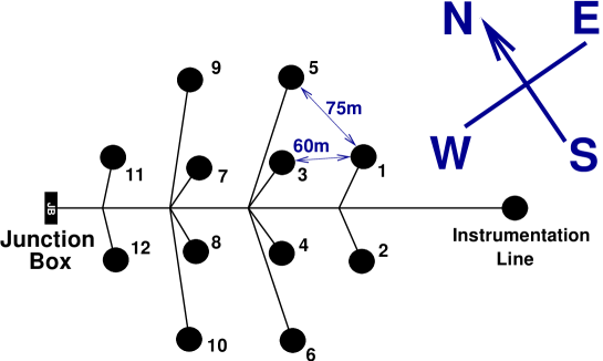
Figure 4.5: Top view of the ANTARES sea floor layout.

4.2 The Optical Modules

The Optical Modules (OMs) are the key elements of the detector. They consist of a pressure-resistant glass sphere of about 43 cm diameter and 15 mm thickness, housing a photomultiplier tube. A photograph of an OM is shown in Figure 4.7. This picture, as well as all other figures in this section, has been taken from [ANT02], where a more detailed description of the OMs can be found.
The photomultiplier tubes (PMTs) ($10^{\prime\prime}$ R7081-20 from Hamamatsu) are glued to the glass spheres with a thin layer of optical silicone gel. A photograph of a PMT is shown in Figure 4.7. A cage made of $\mu$-metal, a nickel-iron alloy with very high magnetic permeability at low field strengths, surrounds the PMT to shield the magnetic field of the Earth. A picture of this cage is shown in Figure 4.8.
The back side of the sphere is painted black to avoid scattered light to reach the PMT from that direction. It houses a penetrator which connects the photomultiplier electronics to the cable leading to the LCM.
The three OMs of one storey are fixed to the OMF with an azimuthal spacing of 120^∘ with respect to each other. In order to increase the sensitivity for upgoing neutrinos, the OMs are looking downward in a 45^∘ angle. The deployment of upward looking OMs would also bear the problem that a layer of sediment material quickly covers the glass spheres; this affects mainly the upper half-sphere, so that a downward looking OM barely encounters any deterioration of sensitivity. The average transmission loss after one year, at 45^∘ from the horizontal, was measured to be around 2% [Pal01b].
Figure 4.9 shows some characteristics of the OM: The quantum efficiency of the PMTs (a) and the measured absorption length of the glass sphere (b) and of the silicone gel (c), all as a function of the wavelength.

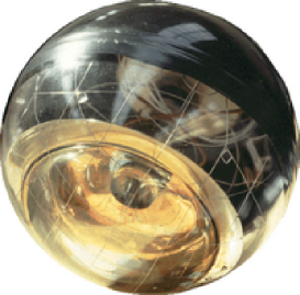
Figure 4.6: Photograph of an OM, taken from [ANT02].

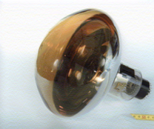
Figure 4.7: Photograph of the $10^{\prime\prime}$ Hamamatsu PMT. From [ANT02].

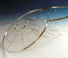
Figure 4.8: The $\mu$-metal cage which is used to shield the Earth’s magnetic field. From [ANT02].

Figure 4.9: Characteristics of the PMTs: quantum efficiency (a), measured absorption length of the glass sphere (b) and of the silicone gel (c). All curves have been plotted as a function of the incident light wavelength. From [ANT02].

4.3 Data Taking in ANTARES

4.3.1 Data Digitisation and Data-Taking Modes

When a photon hits the PMT surface, it produces, with a probability according to the PMT quantum efficiency, a secondary electron which then travels towards the anode; cascades of secondary electrons are produced in the 14 dynodes in-between the photocathode and the anode, yielding an amplification of $10^{7}-10^{9}$ between the cathode and the anode [ANT05d]. The connection between the anode signal, i.e. charge, and the original number of single photo-electrons (pe) can be found in calibration measurements. Figure 4.10 shows such a measurement [ANT05d] for a number of single photo-electron signals (which means that laser pulses with an average number of one photon per pulse were sent to the PMT; with Poissonian probability, also two, three or more photons are present in one pulse. The photo-electrons from the photon pulses are produced according to the quantum efficiency of the PMT.).

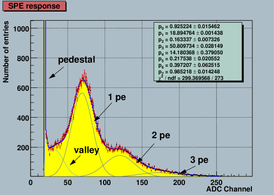
Figure 4.10: PMT response for a single photo-electron signal. The $x$-axis shows the Analogue to Digital Converter (ADC) channel which is proportional to the anode charge; each channel stands for about 0.25 pC charge. The pedestal is the intrinsic noise of the PMT when the signal approaches zero; because of this intrinsic noise, no measurement is possible below a certain threshold, which is usually about 0.3 pe to 0.5 pe (for this study, a minimum pe threshold of 0.3 pe was used). The measured charge for a given number of pe follows a Gaussian probability distribution. The prominent peak in the figure, marked 1 pe, comes from the most probable case that one pe was produced from the photon pulse. The cases where two or three pe were produced can be seen as smaller peaks marked 2 pe and 3 pe. The parameters of a fit function describing the total shape of the histogram are also shown. This figure was taken from [ANT05d].

The conversion of the PMT pulses to digital signals which can be sent to the shore station for further processing and storage is done with the Analogue Ring Sampler (ARS) chip. Each OM is read out by two ARSs, allowing for data-taking in two different modes: The Single Photo Electron (SPE) mode and the Waveform (WF) mode. In SPE mode, charge and time of a single pulse are converted to a digital signal and sent to shore. In WF mode more complex pulse shapes can be recorded; 128 signal samples in 1 ns windows are recorded for one signal in this mode. It therefore requires a much higher band-width, about a factor forty more than the SPE mode. A Pulse Shape Discriminator (PSD) in the ARS is used to switch the data-taking to the WF mode, e.g. in the case of a particularly wide pulse. As will be discussed later, for the detection of shower events, the WF mode is more suitable than the SPE mode, because it allows for a larger dynamical range in the amplitude measurement. In order to obtain a reasonable charge resolution, the ADC settings are chosen such that the maximum number of pe measurable with one ARS in the SPE mode is about 20. For the WF mode, the maximum number of measurable pe, i.e. the saturation level is $\sim$ 200, ten times higher than for the SPE mode.
While registering a signal in SPE mode, an ARS is active for 25 ns. Therefore, if several photons reach the PMT within this time period, they are all integrated as one hit. After these 25 ns, the ARS needs 250 ns to process the data. If another signal reaches the same OM within the dead time, it is recorded by the second ARS. Only the case that both ARSs are in processing mode means dead time for the OM; data-taking is then impossible.
For this study, a saturation of 200 pe was assumed in most cases, because the showers studied in this work generally produce larger amplitudes in the PMTs than muons and are therefore more likely to trigger pulse shapes which would be recorded in WF mode. However, no WF implementation exists in the software at the moment. It was therefore assumed that the signals recorded in the WF mode are taken with the same integration and dead time than in the SPE mode, but at a higher amplitude saturation level.

4.3.2 The Software Trigger

The ANTARES data taking follows the philosophy of “all data to shore”, i.e. all signals recorded in the PMTs are sent to the shore station. The amount of recorded data from the whole detector is about 1 GB per second, depending on the background rate. This data rate is too high to be permanently stored; the aim is therefore to reduce it by several orders of magnitude, selecting those time windows containing physics signals and discarding those containing optical background. This is done by a software algorithm mimicking a hardware trigger, which is thus called Software Trigger [Ren04]. The trigger conditions are based on the assumption that the hits induced in different OMs by a muon or particle shower are correlated, whereas the hits caused by optical background are not. The conditions for correlations are explained in detail in Section 6.4, where they are used as filter conditions for the suppression of the optical background. Correlated hits are collected in so-called clusters. When the cluster has reached its adjustable minimal size (e.g. 4 hits for a background rate of 70 kHz), an event is built by selecting all hits within a time window of 2000 ns around the cluster. If another cluster lies within this time window, the two events are merged. The events are then written to disk. The trigger conditions can be adjusted for a variable background, such that the final storage rate is always about 1 MB/s.

4.4 Optical Properties of the ANTARES Site

4.4.1 Absorption and Scattering

The efficiency of Cherenkov light detection and the accuracy of the muon or shower direction reconstruction depends on the absorption and scattering of the Cherenkov light in the water. These effects are described by the absorption length $\lambda_{abs}$ and the scattering length $\lambda_{scatt}$. $\lambda_{abs}$ and $\lambda_{scatt}$ can be combined to the total attenuation length $\lambda_{att}$, a measure of the overall attenuation of light in water:

$$\frac{1}{\lambda_{att}}=\frac{1}{\lambda_{abs}}+\frac{1}{\lambda_{scatt}}.$$ (4.1)

$\lambda_{att}$ is a function of the wavelength of the light; the relevant wavelength region for the detection of Cherenkov light is between 320 nm and 620 nm, according to the characteristics of the photomultipliers and the glass spheres (see Figure 4.9 in Section 4.2). Measurements in the deep sea have shown that the attenuation length in deep salt water is largest (and therefore, the attenuation itself smallest) at $\sim 460-470$ nm [Pri97]. This is in the region of blue light, and therefore a number of test measurements at the ANTARES site using blue LEDs at a wavelength of 466 nm have been performed [Pal99, Pal01a]. For a detector like ANTARES, the scattered photons are not necessarily lost, and therefore the scattering length is replaced by an effective scattering length which depends on the scattering angle. For the ANTARES site, an effective scattering length between 230 m and 300 m, and an absorption length between 50 m and 69 m for blue light were measured in various sea campaigns [ANT05a]. Figure 4.11 shows absorption length and scattering length, as parameterised in the ANTARES software [Gea00] following the results of the test measurements and a theoretical model for the scattering [Kop83]. Scattering effects are, however, not fully simulated in the software.
For this thesis, attenuation effects were considered at a fixed wavelength of 475 nm, using only the respective absorption length, $\lambda_{abs}\equiv\tau=55$ m.

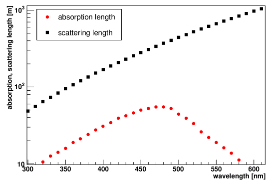
Figure 4.11: Absorption length and scattering length in m at the ANTARES site, as a function of the wavelength, as parameterised in [Gea00].

4.4.2 Refraction Index and Velocity of Light

The refraction index naturally depends on the composition of the medium and hence on the salinity of the water (higher refraction index at higher salinity), its temperature (higher refraction index at lower temperature), and on the water depth (higher refraction index at larger depth, i.e. higher pressure). Typical values of these parameters at the ANTARES site are:

• salinity: $38.44$ ‰;

• temperature: $13.1^{\circ}$C;

• pressure: 200 – 240 bar.

As it connects directly to the velocity of light in water and the Cherenkov angle, a profound knowledge of the refraction index is required. The velocity of light as derived from refraction index measurements is calculated for the ANTARES site in [Pal00]; the value that was found for blue light ($\lambda=466$ nm) is $(0.21755\pm 2\cdot 10^{-5})$ m/ns. The dependence of the refraction index on the various parameters has also been discussed in [Bru00] and is encoded in the Cherenkov light propagation software [Gea00] as a function of the wavelength. Its dependence on the wavelength, for a depth of 2000 m, is shown in Figure 4.12. For this study, a refraction index of 1.3499 was used, which corresponds to a Cherenkov angle of ${\vartheta_{C}=\arccos(1/1.3499)\approx 42.2^{\circ}}$.

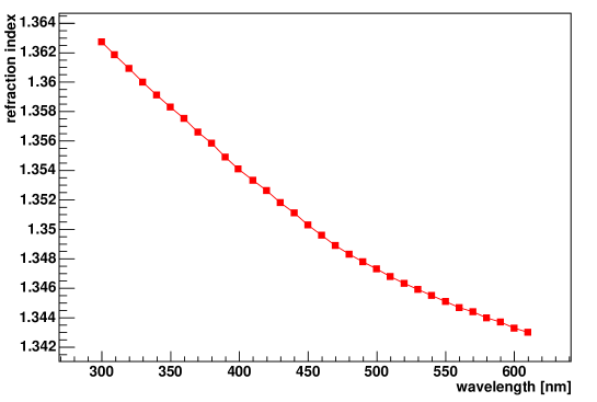
Figure 4.12: Refraction index at the ANTARES site, depending on the wavelength of the Cherenkov radiation, for a depth of 2000 m [Gea00, Bru00].

4.5 Status of the Experiment

Between 1996, the beginning of the ANTARES activities, and 2000, several autonomous lines have been deployed at various sites to measure the optical properties of the water and test the detector components. The most recent of these test lines, recovered in June 2000, also measured signals from atmospheric muons [ANT01].
In October 2001 the main electro-optical cable leading from the ANTARES site to the shore was deployed, followed by the Junction Box, about one year later. Shortly after the Junction Box, a line prototype with five storeys, called Prototype Sector Line (PSL), and the Mini-Instrumentation Line (MIL) were deployed. Both the PSL and the MIL were connected to the Junction Box in March 2003. The MIL was recovered in May 2003 whereas the PSL stayed connected until July 2003.
During that four-month period the PSL took a large amount of data, and the feasibility of the deployment and recovery sea operations was proven. There were some problems, though: Due to a damage of the optical fibre distributing the clock signal, no nanosecond timing was available; also, there was a water leak in the electronics container of the MIL. These problems were thoroughly investigated and eliminated by design modifications. To assure the functionality of the system, two additional test strings, Line 0 and MILOM, were built. Line 0 is a full sized line containing all the mechanical elements of a string, but no electronics. It is used to intensely test the integrity of the mechanical parts of a string during deployment, operation and recovering. MILOM stands for Mini-Instrumentation Line with Optical Modules. The MILOM is an improved version of the MIL; it contains LED beacons for OM calibrations, a hydrophone for acoustic positioning, a sound velocimeter, a conductivity temperature probe, a light transmission meter and a laser beacon. A seismometer is also deployed at 50 m distance, with a connection to the MILOM. Besides these monitoring and control instruments, the MILOM also contains four OMs, three of them arranged on a normal OMF and one of them alone on a separate storey. The smaller buoyancy of the MILOM, as compared to a normal string, is compensated by two buoys. The whole setup is shown in Figure 4.13.

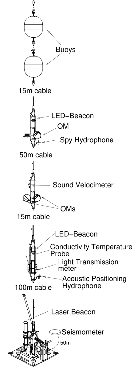
Figure 4.13: Schematic view of the MILOM (Mini-Instrumentation-Line with OMs). See text for more details.

Both Line 0 and MILOM were deployed in March 2005. With the MILOM, a timing resolution better than 1 ns and a positioning resolution of the order of 10 cm was proven [ANT05c]. An example for a measurement of the timing resolution is shown in Figure 4.14. While MILOM is at present still taking data and is foreseen to stay at the ANTARES site to serve as an environmental control instrument for the first complete lines, Line 0 was recovered in May 2005. Leakage tests showed that there were no water leaks in the electronic containers; there were however some optical transmission losses due to an interface problem between EMC penetrators and the LCM. These problems have been understood and solved, and the first complete string has deployed in February 2006 and connected on March, 2nd. The line has been fully functional from the first moment of power-up and the first downgoing muons have been reconstructed. The successful connection of Line 1 is a huge step forward in the completion of the detector planned for the year 2007.

4.6 Other Experiments

The planning of the first neutrino telescopes already started as early as 1975. This section lists high-energy neutrino telescopes of the past, the present and the future, which use the Cherenkov detection technique in water or ice.

• DUMAND
  DUMAND was the pioneering experiment in underwater neutrino detection. It was started in 1975 with the objective to build a neutrino telescope in the deep sea close to Hawaii, USA. Unfortunately, after encountering some technical problems, the experiment was cancelled in 1995 without having taken data. However, the expertise gained in this experiment, theoretically as well as experimentally, has been an extremely useful basis for all later experiments.

• BAIKAL
  The BAIKAL experiment [BAI97] is located at 1070 m depth in Lake Baikal (Russia). It has been the first running high-energy neutrino telescope, with site tests and research and development going on since 1980. The oldest components of the current detector, NT 200+, have been in use since 1993. NT 200+ consists of 8 closely spaced strings plus 3 additional strings in a distance of 100 m to the others. Recently published flux limits of four years of data-taking [Wis05] set a limit of ${E^{2}\Phi<8.1\cdot 10^{-7}\textrm{GeV cm}^{-2}\,\textrm{s}^{-1}\,\textrm{sr}^{-1}}$ for cosmic neutrinos between 10 TeV and 10 PeV (see Figure 4.15).
  The advantage of BAIKAL compared to the other neutrino telescopes is the relatively easy access to the detector. The strings can be deployed and recovered during winter when the surface of the lake is frozen, by melting holes into the ice. It is more easily accessed than the South Pole, and no ship is needed, other than for the experiments in the sea. On the other hand, the optical properties of the water are relatively poor compared to the deep-sea sites in the Mediterranean, with a significantly shorter attenuation length of $\sim 20$ m.

  

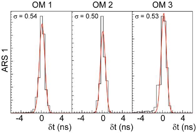
  Figure 4.14: Time distribution of a signal in three OMs of the MILOM, relative to the reference signal of the LED beacon, after subtracting an offset for the light propagation. From [ANT05b].

• AMANDA
  The AMANDA experiment [AMA00] has been built at the South Pole and is operational since 1997. The last stage, AMANDA-II, consists of 677 optical modules mounted on 19 strings which are arranged in concentric circles. The telescope is installed in the glacial ice in depths between 1500 and 2000 m. Using ice instead of water as detector medium has both advantages and disadvantages. In ice, the optical background is very low ($<1$ kHz per optical module) which allows for a lower energy threshold than in water. On the other hand, due to inhomogeneities in the ice, scattering effects are much larger than in water, which deteriorates the resolution, especially for the reconstruction of the neutrino direction. Nevertheless, many important results on neutrino astronomy come from the AMANDA experiment, like stringent limits on diffuse neutrino flux, see Figure 4.15, and for point sources. No evidence for individual sources has been found yet, as can be seen from the recently published results [AMA04b] shown in Figure 4.16. Note that all areas in the plot showing an enhancement of the flux can be explained as statistical fluctuations.
  In spring 2005, the AMANDA experiment has officially become a part of the km³-sized detector IceCube, which is under construction at the same site (see below).

• NESTOR
  NESTOR [NES98] is a neutrino telescope which is being constructed in 4000 m depth off the Greek coast. Other than ANTARES, it uses a rigid structure of towers, each consisting of 12 floors which carry 12 OMs each. The OMs are symmetrically orientated upwards and downwards, which allows for a uniform angular acceptance, such that the background from above can be studied. A first test floor of reduced size has been successfully deployed and operated in 2003 [NES05a, NES05b].
  

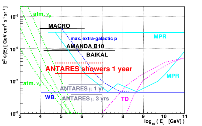
Figure 4.15: Neutrino flux limits reached or expected with different neutrino experiments, and predicted bounds [Bah99, Bah01, Man00, Sig98]. ANTARES expectations from [Zor04], Macro limit from [MAC03], BAIKAL limit from [Wis05], AMANDA limit (for cascades) from [AMA04a]. See Figure 3.10 in Section 3.3 for details on the theoretical predictions.

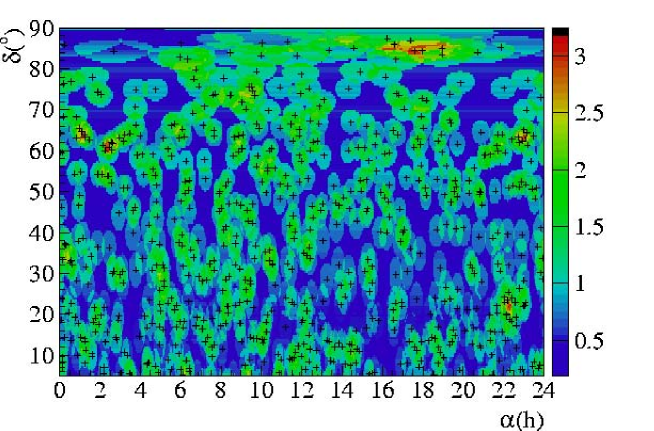
Figure 4.16: AMANDA upper limits (90% C.L.) on the neutrino flux integrated above 10 GeV in equatorial coordinates, declination $\delta>5^{\circ}$ over right ascension $\alpha$ (in hours), in units of $10^{-8}$ cm^-2 s^-1 (colour-coding on the right). The data were taken in the years 2000-2002, and an $E^{-2}$ spectrum has been assumed. The cross symbols represent the observed events. From [AMA04b].

The size of the neutrino telescopes mentioned above, about 0.01 km³, will only allow to measure a few high-energy events per year, because the fluxes are so small. As will be explained in Section 5.1, some types of events, e.g. the tau double bang events, will even be difficult to detect at all, due to their large extension in comparison to the detector size.
To be able to collect data with a higher statistical significance, larger volumes are needed. Therefore, km³-sized detectors are being planned or under construction:

• NEMO
  The NEMO collaboration [NEM05] is doing research and development with regard to a future km³ detector in the Mediterranean. A candidate site for the km³ detector, 70 km off the Sicilian coast in a depth of 3500 m, has been identified and exhibits good optical properties.

• KM3NeT
  KM3NeT is a consortium formed by the members of the three neutrino experiments in the Mediterranean, ANTARES, NEMO and NESTOR, with the objective to build a km³-sized detector in the Mediterranean. The location on the Northern Hemisphere is complementary to the site of Antarctic IceCube detector (see below) to allow for the observation of the Southern sky, including a large part of the Galactic disc and the Galactic Centre, which is barely visible with IceCube.
  The experiment is now in its R&D phase; a design study funded by the European Union is currently being conducted. In the course of this, the technical design will be worked out.

• IceCube
  IceCube [Ice01] is the km³-sized extension to the AMANDA neutrino telescope in the Antarctic Ice. Nine strings have been deployed since the Antarctic summer 2004/2005, and the completion of the detector is expected for 2011. The detector will then consist of 4800 photomultiplier tubes on 80 lines, each of them over 1000 m long, with a horizontal spacing of 125 m to each other. On the surface, an air shower array, IceTop, is being built, which will serve for calibration purposes and as a veto for atmospheric muons.

Chapter 5 Signal Events in ANTARES

This chapter is devoted to the different classes of signal events that occur in the ANTARES detector, with a particular weight on shower-type events.
Section 5.1 provides a closer look at the signatures of the different event classes. In Section 5.2, details on the characteristics of electromagnetic cascades are given. Section 5.3 provides similar information for hadronic cascades.
The Monte Carlo results shown in this chapter are mostly obtained using ANTARES simulation software. See Appendix A for a more detailed description of this software.

5.1 The Different Event Classes in ANTARES

In an electromagnetic field-free environment, charged particles travel along straight lines through the medium until they either decay or interact with the interaction medium. The mean length of the distance travelled is called the path length of the particle and depends on its amount of energy loss in the medium. If the path length exceeds the spatial resolution of the detector, so that the trajectory of the particle can be resolved, one calls the trajectory a particle track. In a neutrino telescope, one can distinguish between two main event classes: events with a track, and events without a track.

5.1.1 Event Classes with a Track

Event classes with a track are

• $\nu_{\mu},\bar{\nu}_{\mu}$ CC:  $(\nu_{\mu},\bar{\nu}_{\mu})+N\to\mu^{\mp}+$ hadronic shower

• $\nu_{\tau},\bar{\nu}_{\tau}$ CC:
   $(\nu_{\tau},\bar{\nu}_{\tau})+N\hskip 1.28036pt\to$ hadronic shower $\hskip 1.13809pt+\,(\tau^{\mp}\to(\nu_{\tau},\bar{\nu}_{\tau})+(\bar{\nu}_{\mu},\nu_{\mu})+\mu^{\mp})$
   $(\nu_{\tau},\bar{\nu}_{\tau})+N\to$ hadronic shower $+\,(\tau^{\mp}\to(\nu_{\tau},\bar{\nu}_{\tau})+(\bar{\nu}_{e},\nu_{e})\,+\,(e^{\pm}\to$ em. shower))  $(\nu_{\tau},\bar{\nu}_{\tau})+N\hskip 1.28036pt\to$ hadronic shower $\hskip 1.13809pt+\,(\tau^{\mp}\to(\nu_{\tau},\bar{\nu}_{\tau})\hskip 2.84526pt+$ hadronic shower).
  

The last two channels only produce tracks within certain energy ranges, see below. In the list, “em. shower” stands for electromagnetic shower. Schematic views of a $\nu_{\mu}$ CC event and of the last of the three $\nu_{\tau}$ CC channels are shown in Figure 5.1. Neutrino and anti-neutrino reactions are not distinguishable; thus, no differentiation between particles and anti-particles is made. Showers occur in all event classes shown in Figure 5.1. However, for $\nu_{\mu}$ and $\bar{\nu}_{\mu}$ CC, often only the muon track is detected, as the path length of a muon in water exceeds that of a shower by more than 3 orders of magnitude for energies above $\sim 2$ TeV (see Figure 5.2). Therefore, such an event might very well be detected even if the interaction has taken place several km outside the instrumented volume, provided that the muon traverses the detector.
Because of its highly relativistic velocity, the muon undergoes a large number of interactions before it decays. For energies above $\sim 2$ TeV, these interactions are dominated by radiation losses.
For the $\tau$, the situation is different: due to the much shorter lifetime, it travels only a few m to a few km, depending on its energy, before it decays again according to one of the possible decay modes given in the list above. Radiation losses, on the other hand, play a much smaller role than for the muon, because of the 17 times larger mass of the $\tau$. Most of the possible $\tau$ decay modes include the generation of a hadronic or electromagnetic cascade. Thus, if the track of the $\tau$ is long enough to distinguish between the primary interaction of the $\nu_{\tau}$ and the decay of the tau, i.e. for a $\tau$ energies above $\sim 1$ PeV (see Figure 5.2), the expected signatures for the $\nu_{\tau}$ and $\bar{\nu}_{\tau}$ CC events are that of a shower, a track and a shower; this signature is called “double bang event”. Alternatively, if the $\tau$ starts or ends outside the instrumented volume, a track and a shower, a “lollipop event”, are detected. Most probably, if events at these high energies are observed in ANTARES at all (the expected event rate above 1 PeV is far below 1 event per year), this latter signature is the only one observable in ANTARES, because the tau path length rapidly exceeds the dimensions of the detector for increasing energies.
If the $\tau$ decays into a muon, a $\nu_{\tau}$ and a $\nu_{\mu}$, the event is presumably not distinguishable from an original $\nu_{\mu}$ CC interaction.

Figure 5.1: Schematic view of the most important event classes in ANTARES, as described in the text: $\nu_{\mu}$ CC (a), $\nu_{\tau}$ CC (“double bang event”) (b), $\nu_{e}$ CC (c) and $\nu$ NC (d).

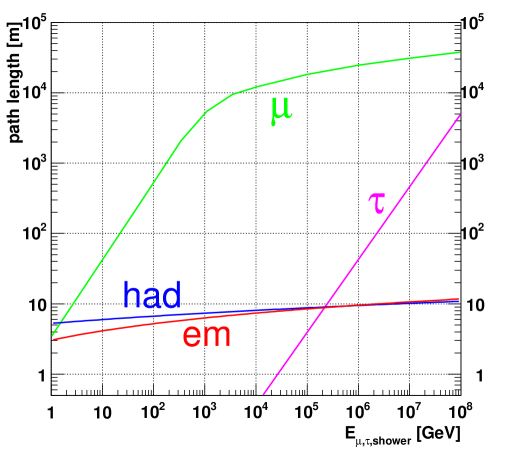
Figure 5.2: Path length of neutrino interaction products in water: muons, taus, electromagnetic and hadronic showers, over their respective energy. The shower lengths are calculated using a shower profile parameterisation and the results of [Nie05], see Section 5.3 for details. Muons and taus after [Iye01].

5.1.2 Event Classes without a Track

Event classes without a track are

• $(\nu_{e},\bar{\nu}_{e})$ CC:  $(\nu_{e},\bar{\nu}_{e})+N\to$ hadronic shower $+\,(e^{\mp}\to$ electromagnetic shower)

• $(\nu,\bar{\nu})$ NC:     $(\nu_{l},\bar{\nu}_{l})+N\to(\nu_{l},\bar{\nu}_{l})+$ hadronic shower

Both event classes are depicted schematically in Figure 5.1. Due to its small mass, the electron has a high probability for energy loss via bremsstrahlung, so that it does not produce a resolvable track in the detector, but interacts immediately after its generation, producing an electromagnetic shower.
The NC channel gives the same signature for all neutrino flavours. In this channel, a part of the interaction energy is always carried away unobserved by the outgoing neutrino, and therefore the error on the reconstructed energy of the primary neutrino increases accordingly. Even though electromagnetic and hadronic showers are different from each other in principle (see Sections 5.2 and 5.3), the $\nu_{e}/\bar{\nu}_{e}$ CC and the $\nu$ NC channels are not distinguishable in reality, because the detector is too sparsely instrumented.
Below $\sim 1$ PeV, also the $\nu_{\tau}$ CC channels, except for the case where the $\tau$ produces a muon, belong to the class of events without a track, because the $\tau$ track cannot be resolved at these energies (see Figure 5.2).

5.1.3 Other Event Classes

The resonance channel of $\bar{\nu}_{e}$ at 6.3 PeV, the Glashow resonance, is a special case which is mentioned here for completeness. The following signatures are possible for this resonance:

• $\bar{\nu}_{e}+e^{-}\to\bar{\nu}_{e}+(e^{-}\to$ electromagnetic shower)

• $\bar{\nu}_{e}+e^{-}\to\bar{\nu}_{\mu}+\mu^{-}$

• $\bar{\nu}_{e}+e^{-}\to\bar{\nu}_{\tau}+(\tau^{-}\to\tau^{-}$ decay modes (see Section 5.1.1) )

• $\bar{\nu}_{e}+e^{-}\to q+\bar{q\,}^{\prime}\to$ hadronic shower

For the energy range examined in this study, between $\sim 100$ GeV and $\sim 100$ PeV, the resonance channel constitutes only a small portion to the overall cross section. It will also not be identifiable as such in the experiment: In the case of $\bar{\nu}_{e}+e^{-}$ or $q\bar{q\,}^{\prime}$ final states, the interaction has the same characteristics as a “normal” shower event without a track. As it is presumably not possible to determine between a track traversing the detector and a track starting inside the detector, neither of the two other channels will be identifiable: In the case of $\bar{\nu}_{\tau}+\tau^{-}$, the interaction would be regarded as a $\bar{\nu}_{\tau}$ CC with the primary neutrino interaction outside the detector and in the case of $\bar{\nu}_{\mu}+\mu^{-}$, the only event type without any shower, it would be interpreted as a $\nu_{\mu}$ CC event happening outside the detector. In a larger, km³ sized detector, this would be different, because it would be possible to determine whether a particle track starts within the instrumented volume or outside of it. For ANTARES, where the majority of the strings are situated at the edge of the detector (see Figure 4.5 in Section 4.1), this seems very improbable.

5.1.4 Event Classification

Figure 5.3 shows two different Monte Carlo events in the ANTARES detector in comparison. On the left, the passage of a muon (blue) through the detector is shown. The muon is travelling from the lower right to the upper left in the shown perspective; its initial energy was 19 TeV. On the right, an NC interaction is shown; the neutrino, marked in black, comes from the upper right and interacts in the middle of the detector, generating a hadronic shower (blue). The energy of the hadronic shower was also 19 TeV. Note that the shower constituents have been extrapolated according to their directions; the length of the lines is not to scale. The events have been visualised using the ANTARES event display A3D [Hei05]. The storeys in the strings are drawn as small dots; the photomultiplier signals, integrated over 25 ns, are shown as squares, with a size proportional to the signal amplitude, and a colour coding according to the arrival time of the photon signal in the photomultipliers (yellow to green to light blue).
One can clearly see that the shower deposits its entire energy in a relatively small volume, while the muon loses only a part of its energy inside the detector.

Figure 5.3: Passage of a muon through the ANTARES detector (left) and an NC interaction inside the detector (right), as visualised by the ANTARES event display A3D [Hei05]. The shower length is not to scale. See text for details.

5.2 Electromagnetic Cascades

The evolution of an electromagnetic cascade can be described in a very simple way: An electron suffers bremsstrahlung and produces photons. Each photon produces an electron-positron pair via pair production. The electron and the positron again produce photons via bremsstrahlung, and so on, until the energy of the constituents falls below the critical energy and the shower production stops; the remaining energy is then dissipated by ionisation and excitation. For electromagnetic showers it can be assumed that all Cherenkov light is emitted isotropically in azimuth $\phi$ from the shower axis, as the lateral extension of an electromagnetic shower is of the order of 10 cm [Eid04] and therefore negligible in comparison to the longitudinal one. Thus, the description of an electromagnetic shower simplifies to describing the longitudinal profile of the shower and the angular profile of the emitted Cherenkov light.

5.2.1 Longitudinal Profile

The longitudinal profile of the energy deposition in the shower can be parameterised as [Eid04]

$$\frac{dE}{dt}=E_{0}b\frac{(bt)^{a-1}e^{-bt}}{\Gamma(a)},$$ (5.1)

where $E_{0}$ is the initial shower energy, $a$ and $b$ are parameters depending on the initial energy and particle type, and $t$ is the distance from the interaction vertex along the shower axis in units of radiation lengths, $t=z/X_{0}$, with $X_{0}=35$ cm in salt water at the ANTARES site [Bru02]. One finds that the maximum of distribution (5.1) is at

$$t_{max}=(a-1)/b.$$ (5.2)

The parameters $a$ and $b$ for electron- and photon-induced interactions in salt water have been determined by various authors [Wie95, Bru02, Nie05]. Their results are listed in Table 5.1, showing good compatibility within the typical precision of around 10%, except for the slightly larger constant offset of [Nie05]. Note that [Nie05] uses a different form of equation (5.2), $t_{max}=D\ln(E/E_{c})+C$, from which the expression for $a$ can be calculated using the values cited for $b$ and a critical energy of $E_{c}=54.27$ MeV. The numbers given here are valid up to $\sim 1$ PeV; above this energy, the LPM effect, a suppression of pair production and bremsstrahlung, has to be taken into account. [Nie05] uses the GEANT4 [Gea05] simulation software to simulate the particle interactions in water, while the other two have done their simulations with the older version GEANT3.21 [Gea93].

	shower parameter $a$		shower parameter $b$
author	$e^{-}$	$\gamma$	$e^{-}$	$\gamma$
[Wie95]	$2.0+0.60\ln(E/\textrm{GeV})$	(not calculated)	0.63	(not calculated)
[Bru02]	$1.9+0.64\ln(E/\textrm{GeV})$	$2.6+0.64\ln(E/\textrm{GeV})$	0.66	0.66
[Nie05]	$2.6+0.69\ln(E/\textrm{GeV})$	$3.4+0.74\ln(E/\textrm{GeV})$	0.69	0.74

Table 5.1: Mean value of the longitudinal shower profile parameters $a$ and $b$ for electrons and photons, as determined by various authors. The value of $b$ cited for [Bru02] was obtained by calculating the mean from the values given for different energies; the author himself used $b=0.64$ to obtain parameter $a$. $b$ is expected to be constant in energy and identical for electrons and photons.

As an example, the longitudinal profiles for electron-induced showers at 100 GeV, 1 TeV, 10 TeV, 100 TeV and 1 PeV, using the values from Table 5.1, are shown in Figure 5.4. The shapes of all distributions are very similar to each other, but the positions of the curves derived from [Nie05] are shifted to higher values of $t$.

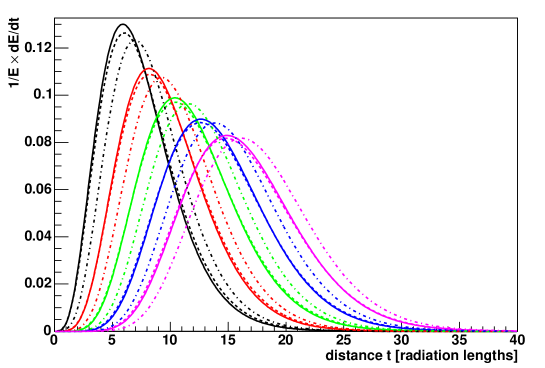
Figure 5.4: Longitudinal profiles of electron-induced showers at energies of 100 GeV (black), 1 TeV (red), 10 TeV (green), 100 TeV (blue) and 1 PeV (magenta), as parameterised by [Wie95] (dashed lines), [Bru02] (solid lines) and [Nie05] (dashed-dotted lines).

The longitudinal profiles are used to parameterise the total shower length as a function of the initial shower energy. The shower length is defined here as the distance within which 95% of the total shower energy has been deposited. Integrating the curves shown in Figure 5.4 numerically, and parameterising the results as linear functions in $\log_{10}(E)$, one obtains the expressions for the shower length listed in Table 5.2; again, the agreement of the results is within 10%.

author	path length $L$ [m]
[Wie95]	$2.93+1.04\log_{10}(E/$GeV )
[Bru00]	$2.79+1.06\log_{10}(E/$GeV )
[Nie05]	$3.04+1.09\log_{10}(E/$GeV )

Table 5.2: Path length $L$ for electron-induced showers as a function of the shower energy, parameterised using the results given by the different authors.

For this study, the values of [Nie05] have been used to retrieve the shower length and the position of the maximum, because they are the most recent ones; the new GEANT4 simulation uses new results for the cross sections at high energies, which makes its output more reliable than that obtained with the older version, GEANT3.21. See Figure 5.2 in Section 5.1 for a graphical representation of the electromagnetic shower length as a function of the shower energy.

5.2.2 Angular Profile

It has been found both by [Wie95] and by [Bru02] that above 1 GeV, the distribution of the Cherenkov photon radiation angle $\vartheta_{C}$ with respect to the shower axis is energy-independent for electromagnetic showers, and very well reproduceable from event to event. It is therefore possible to save computing time during the shower simulation by calculating the total number of emitted Cherenkov photons according to the shower energy and assuming a fixed angular profile for the photons, instead of producing the photons separately for each shower particle. In the ANTARES simulation software (see Appendix A.2), this has been done by parameterising the angular distribution in the region of $\cos\vartheta_{C}<0.4$, i.e. $\vartheta_{C}\gtrsim 66^{\circ}$, following the results of [Bru02] for the simulation of electromagnetic showers. The region of smaller angles is hard-coded in the simulation package, with a bin width of $1\times 10^{-3}$ in $\cos\vartheta_{C}$. The overall distribution obtained that way is shown in Figure 5.5.

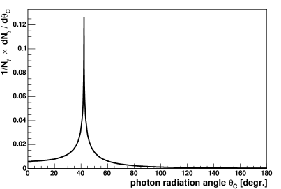
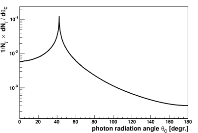
Figure 5.5: Angular distribution of photons in an electromagnetic shower with respect to the shower axis, as parameterised within the ANTARES simulation software (see Appendix A.2), following the studies of [Bru02]. Left: linear $y$-scale, right: logarithmic $y$-scale.

5.3 Hadronic Cascades

The description of hadronic cascades is less straight-forward than that of electromagnetic ones, the main reason being that event-to-event fluctuations are much more important in hadronic showers, since they do not consist only of two particle types like electromagnetic cascades, but of many, and the fraction of the different particle types depends on the shower energy. The dominant secondary particles in a hadronic shower are pions; other hadrons like kaons, protons or neutrons occur in variable fractions. A number of muons can be present, as well; as these usually leave the shower producing long tracks, they contribute significantly to the fluctuations. For increasing shower energy, the electromagnetic component in the hadronic shower increases, because the number of $\pi^{0}$ increases significantly, due to the interactions of the charged pions; at lower energies, these charged pions decay before they can interact, producing mainly muons. $\pi^{0}$ have a much shorter lifetime than charged pions and decay into two photons; these photons are then the origin of an electromagnetic cascade. The percentage of electrons or positrons on the total track length of a hadronic shower exceeds 90% for a shower energy of 1 TeV [Bru02], which means that above this energy, the largest part of the Cherenkov light in the shower is generated by electromagnetic sub-showers.
Figure 5.6 shows the relative abundance of shower particles for different shower energies, as simulated by the ANTARES neutrino interaction package (see Appendix A.1). The output of this simulation consists of all long-lived particles, i.e. particles with a lifetime $\gtrsim 10^{-10}$ s, so that e.g. $\pi^{0}$ occur only through the photons that have been produced in their decays. Consequently, the photon abundance in the shower is very high. Note also that only the primary shower particles are displayed here; e.g. secondary electrons produced during cascading, or Cherenkov photons, are not displayed, as they are not generated at this simulation step, but only in the propagation that follows.

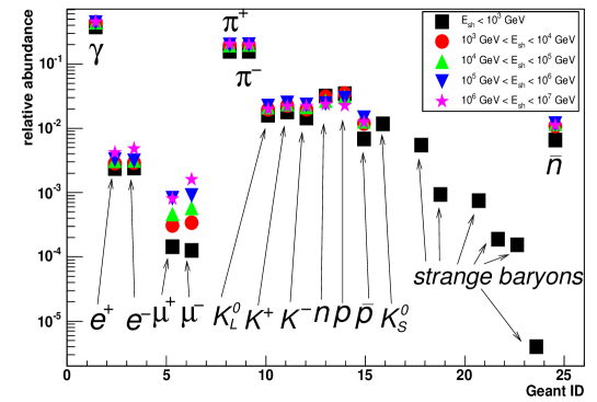
Figure 5.6: Composition of hadronic showers: relative abundance of secondary particles in hadronic showers with different primary energies, as simulated by the ANTARES event simulation software genhen (see Appendix A.1). Note that only long-lived particles are displayed by the simulation software.

5.3.1 Longitudinal Profile

One of the authors mentioned in the previous section, [Nie05], has used his parameterisation for the electromagnetic showers, equation (5.1), also to determine the longitudinal profile of hadronic showers. He simulated the hadronic cascade generated by a primary charged pion at different energies. The values he finds for the parameters $a$ and $b$ are given in Table 5.3. The resulting longitudinal profiles from this parameterisation are shown in Figure 5.7 for shower energies of 100 GeV, 1 TeV, 10 TeV, 100 TeV and 1 PeV, in units of the electromagnetic radiations length in salt water, $X_{0}=35$ cm, to allow for a comparison with the electromagnetic showers. The profiles for electron-induced showers at the same energies, following the results of [Nie05], are shown as dashed-dotted lines in the same figure. Below 100 TeV, the electromagnetic shower has a shorter length than the hadronic shower. While the shower maximum for electromagnetic showers with energies $\geq 100$ TeV lies at a larger distance from the interaction vertex than for hadronic showers, the overall shower length becomes approximately equivalent for both shower types (compare Figure 5.2).
Due to the increasing electromagnetic component, fluctuations in the hadronic shower shape are less dominant at higher energies. [Nie05] finds that the fluctuations with respect to the longitudinal profile are around 10% at some 10 TeV; they exceed 30% in the region of some hundred GeV. The shower parameter $b$ showed no constant behaviour below $\sim 5$ TeV. For shower energies in this energy region, the parameterisations presented here should therefore be used with care.

parameter	$\pi^{\pm}$
$a$	$4.26+0.364\ln(E/\textrm{GeV})$
$b$	0.56 ($E\geq 10$ TeV)

Table 5.3: Mean value of the longitudinal shower profile parameters $a$ and $b$ for charged pions, as determined by [Nie05]. The parameter $b$ is expected to be constant in energy.

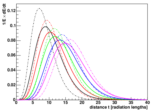
Figure 5.7: Longitudinal profiles for a pion-induced hadronic shower at energies of 100 GeV (black), 1 TeV (red), 10 TeV (green), 100 TeV (blue) and 1 PeV (magenta) (solid lines), as parameterised by [Nie05]. The longitudinal profiles for an electron-induced shower as parameterised by [Nie05] at the same energies are shown as dashed-dotted lines, for comparison.

One can again use the longitudinal profile, as explained in Section 5.2, to parameterise the total shower length. The shower length $L$ was again defined as the distance within which 95% of the total shower energy is deposited. It can be described as

$$L/\textrm{m}=5.28+0.70\log_{10}(E/\textrm{GeV}).$$ (5.3)

The length of a hadronic shower using equation (5.3), in comparison to the electromagnetic shower length and the muon and $\tau$ ranges is shown in Figure 5.2 (Section 5.1).
The maximum of the shower retrieved from Table 5.3 was compared to the shower maximum as calculated in a study that was conducted within the context of this thesis. For this study, the ANTARES simulation tools (see Appendix A) were used to generate a sample of NC events with shower energies between $\sim 40$ GeV and $\sim 100$ PeV. In the following, this event sample will be denoted event sample A (Appendix A.5 gives a detailed description of the different event samples that were used for this work).
The output of the Monte Carlo simulation contains no information about the longitudinal extension of the shower and thus, no information about the position of the shower maximum is available. However, from the timings and positions of the measured hits, one can reconstruct the point from where the largest fraction of Cherenkov photons is emitted, according to an algorithm described in Section 7.1. Here and in the following, the term hit is used to denote a set of photons which reach a photomultiplier within the 25 ns integration time that follow the first photon signal in the photomultiplier (see Section 4.3.1). The number of photo-electrons (pe) in a hit determines the hit amplitude. Taking into account the hit amplitudes for the calculation, by weighting each hit position and time by its amplitude, a centre-of-gravity of the shower, $\vec{r}_{\text{CGA}}$, can be determined as an estimate of the central point of photon emission. This centre-of-gravity is approximately equivalent to the shower maximum, as can be seen from Figure 5.8: On the left hand side, the distance $\Delta r$ between the interaction vertex and $\vec{r}_{\text{CGA}}$, calculated as described above, is shown in red for each event. On the right hand side, the profile of the calculated data points is shown. A straight line that was fitted to this profile is shown in green in both graphs. The length of the line marks the validity range of the fit. For energies below $\sim 1$ TeV, the event-to-event fluctuations begin to dominate the distribution. The fit function is given as

$$\Delta r(E)/\textrm{m}=3.7+0.20\log_{10}(E/\textrm{GeV}).$$ (5.4)

The position of the shower maximum with respect to the interaction vertex, as expected from the simulations of [Nie05], is shown in blue in both graphs. The agreement between the two lines is relatively good, considering the different methods that were used, though the increase of the fit line with energy is not as strong as predicted by [Nie05]. It should also be noted that the shower maximum may not necessarily be equivalent to the point of maximum photon emission.

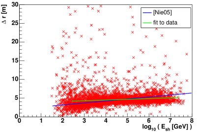
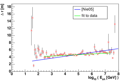
Figure 5.8: Distance between the MC interaction vertex and the amplitude-weighted centre-of-gravity $\vec{r}_{\text{CGA}}$ as calculated for the NC event sample A, a fit to the data (green), and distance between the MC interaction vertex and the position of the shower maximum as predicted by [Nie05] (blue), all as a function of the shower energy. See text for details.

5.3.2 Angular Profile

Same as the longitudinal shower profile, also the angular profile of the Cherenkov photons suffers from large fluctuations for hadronic showers, in particular for low energies. Considering different energies, it also becomes obvious that the angular distribution slightly broadens with increasing energy, which might by due to the increasing total number of particles in the shower. Figure 5.9 shows the angular distribution for showers between $3\times 10^{2}$ and $3\times 10^{7}$ GeV from event sample A; each histogram contains events within one decade in energy. Shown is the angle between the photons which produced a hit in the ANTARES detector and the shower axis. The angle was calculated under the assumption that all photons are emitted from one point in the shower. It will be shown later in Section 7.1 that the position reconstructed by the algorithm used for this study does not refer exactly to the shower maximum, but to a distance to the interaction vertex that can be parameterised using equation (7.8) from Section 7.1. The point of the photon emission was therefore calculated by moving the reference point from the Monte Carlo (MC) interaction vertex according to ${2.8+0.48\cdot\log_{10}(E/\textrm{GeV})}$ along the shower axis. Effects due to detector geometry characteristics can not be fully excluded but are expected to cancel out due to large statistics and an isotropic event sample.
In Figure 5.9, the parameterisation of the angular profile for electromagnetic showers (dashed line) as determined by [Bru02] (see Section 5.2), is also shown for comparison. Close to the Cherenkov peak, the distribution does not differ much the one for hadronic showers; it lies below the histogram of the hadronic showers with the lowest energy, for angles between the maximum and $\sim 100^{\circ}$. This agrees with the expectation that the angular distribution is narrower for an electromagnetic shower than for a hadronic shower, as no energy dependence was found for the distribution of the electromagnetic shower. However, for angles below $\sim 35^{\circ}$ and above $\sim 130^{\circ}$ (depending on the shower energy), the photon yield for the hadronic shower is found to lie below the photon yield for the electromagnetic shower and is therefore probably underestimated with the method used here. This effect is possibly caused by the fact that especially low Cherenkov thresholds of $<1$ MeV were used for electrons and photons in [Bru02], while for the angular distributions of the hadronic showers retrieved in this study, the nominal value in the ANTARES software [Gea00] for the high-energy mode, 500 MeV, was used to save computing time. One should also be aware that what is compared here is on the one side a photon distribution of electromagnetic showers which has been retrieved from the Monte Carlo truth of the Cherenkov photon simulation, and on the other side distributions of photo-electrons from hadronic showers as measured in the detector according to the ANTARES simulation software.

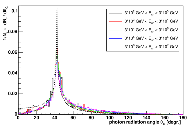
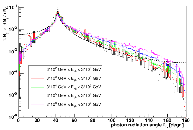
Figure 5.9: Angular distribution of photons from a hadronic shower with respect to the shower axis for different energies. Top: linear vertical scale, bottom: logarithmic vertical scale. The angular distribution for electromagnetic showers as parameterised by [Bru02] is shown as a dashed line for comparison. See text for details.

5.3.3 Angle Between Neutrino and Hadronic Shower

One of the important objectives in reconstructing a neutrino event is to determine the direction of the neutrino. In case of the NC events, one has no information about the outgoing neutrino, so that the only object which can be reconstructed is the hadronic shower. However, the direction of the hadronic shower is very similar to the direction of the incoming neutrino, as can be seen in the upper plot of Figure 5.10 for events from event sample A. Here, the direction of the shower was calculated by summing over the directions of all particles in the shower as given by the simulation (see Figure 5.6), each particle weighted with its respective MC energy. One can see that above $\sim 1$ TeV the angular difference between the shower and the neutrino falls below $2^{\circ}$, which is the best value that the resolution for the direction reconstruction of a shower can reach (see Chapter 10; for energies smaller than 1 TeV, the intrinsic resolution is worse). Therefore, within the acquired precision, one can safely regard the shower direction as identical to the neutrino direction.
In the lower plot of Figure 5.10, the same is shown for the case of $\nu_{e}$ CC events, for a subsample of the event sample described in Appendix A.5.2. In this event class (see Section 5.1), an electromagnetic and a hadronic shower are produced. However, these two are not separable in the detection, and therefore, a common shower axis from all particles in the two showers has been calculated by the method described above. This axis is almost identical to the neutrino axis; for the lower energies, inaccuracies of simulation and method cause the small difference between the neutrino and the common shower axis, while above 1 PeV, the size of the calculated angle reaches the precision of the directions in the event sample, and therefore the distribution flattens. The cutoffs at 100 GeV and 10 PeV mark the energy region within which the neutrinos were produced.

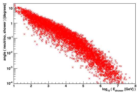
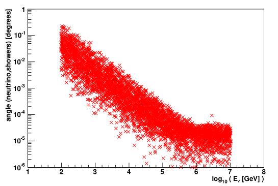
Figure 5.10: Top: Angle between the neutrino and the hadronic shower, in degrees, as a function of the shower energy, for NC interactions. Bottom: Angle between the neutrino and the common axis of electromagnetic and hadronic shower, in degrees, as a function of the neutrino energy, for $\nu_{e}$ CC interactions. See text for details.

Chapter 6 Background

The ANTARES experiment is constructed in the deep sea to suppress as well as possible the background caused by cosmic rays. However, atmospheric muons and neutrinos are present as background at the ANTARES site, and the deep-sea surroundings add additional background sources.
The most dangerous background for $\nu_{\mu}$ CC events (which are reconstructed using the neutrino-induced muon) are atmospheric muons; they can be distinguished well from shower events, so that the latter are much less affected by this background source than $\nu_{\mu}$ CC events, which can only be identified as such if the neutrino comes from below. Atmospheric muons are a potential background for shower events only in two cases: If they experience catastrophic bremsstrahlung losses during their passage through the detector, or if they occur in bundles of several muons crossing the detector at the same time. Atmospheric muons are covered in Section 6.1.
Atmospheric neutrinos, on the other hand, are an irreduceable background for the detection of high-energy cosmic neutrinos, for all event types. Characteristics of atmospheric neutrino fluxes are given in Section 6.2.
A third type of background is the noise from the detector medium itself, the deep sea. Decays of ⁴⁰K nuclei in the salt water produce a constant background rate of one-photon signals; multi-cellular organisms add high bursts erratically. The different types of this optical noise are discussed in Section 6.3, whereas methods for its suppression are introduced in Section 6.4.

6.1 Atmospheric Muons

Atmospheric muons are produced in interactions of high-energy cosmic rays in the atmosphere, through the decay of secondary mesons. The production chain is the same as the one discussed for the production of neutrinos (see equation (2.1) in Section 2.3.2). Atmospheric muons are produced abundantly in the atmosphere, and at energies above $\sim 1$ TeV their free path in water is long enough to reach the detector in 2400 meters depth (see Figure 5.2 in Section 5.1). They present a serious background to the detection of muons from $\nu_{\mu}$ CC interactions, as they exceed the muon rate from atmospheric neutrinos by several orders of magnitude (see Figure 6.3). For the detection of neutrino-induced muons it is therefore necessary to restrict the analysis to events coming from below.
Owing to the different topology of muon events and shower events (see Section 5.1), the situation is different for showers. It is, however, possible that an atmospheric muon suffers a strong radiative loss, a so-called catastrophic energy loss, which means that it radiates a substantial fraction of its energy into one secondary photon, which in turn produces an electromagnetic cascade. If the energy of the cascade exceeds a few 100 GeV, it can be detected and hence be confused with a cascade from a neutrino interaction.
The average energy loss of muons is shown in Figure 6.1 for copper as target medium. One can see that for energies in the TeV region, radiative losses are by far the dominating mechanism.

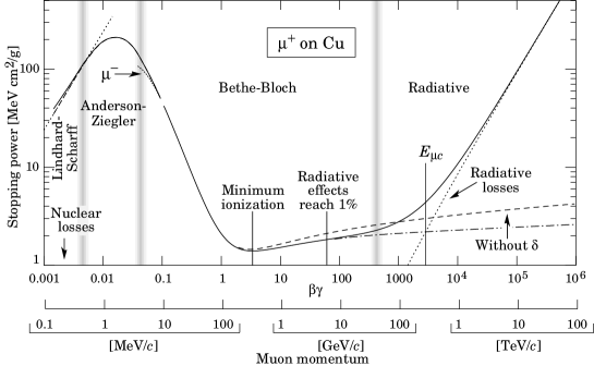
Figure 6.1: Stopping power (i.e. avarage energy loss) of muons in copper. The shape curve is equivalent for other media but shifted in energy; the critical energy $E_{\mu c}$ lies at 1 TeV for water. The dashed line marked “without $\delta$”  refers to the omission of density effect corrections to the ionisation energy loss. From [Eid04].

The second background type caused by atmospheric muons are multi-muon events, where a bundle of muons generated by one primary cosmic ray passes the detector, so that their signals in the detector are causally connected. These events could be misinterpreted as shower-type events as well, especially if the muon multiplicity is high, because in this case a large amount of electromagnetic radiation could be produced, which could then be misinterpreted as a neutrino-induced shower. For protons as primary cosmic rays, the muon multiplicity $M$ at sea level depends on the proton energy $E$ approximately according to a power-law: ${M\propto E^{0.83}}$ [Suk03]. The more energetic the cosmic rays are, the larger is thus the probability that they produce a muon bundle. A similar correlation between multiplicity and primary energy was also found for iron primaries, but with a multiplicity that is about an order of magnitude higher than for the primary protons. It is assumed that the multiplicity distributions for the other primaries with masses between protons and iron are in between these two distributions. The decrease of the muon flux with increasing water depth can be seen in Figure 6.3, for different muon multiplicities, as calculated by [Mar05a]. The fluxes shown in the figure refer to vertical muon bundles from a combined simulation of five different types of primaries. Note that increasing water depth leads to a suppression of the flux, but only to a weak change in the multiplicity ratios. At the depth of the ANTARES detector, marked by the yellow area, the flux of single muons is about a factor of 80 higher than that of bundles with more than four muons.
As these two event types imitate neutrino-induced showers, they will not be recognised as background in the reconstruction, but must be suppressed afterwards. This suppression, together with event rates, will be discussed in Section 9.1. It will be shown there that the relation between single muons and muon bundles is modified significantly in the reconstruction, as the events with a high muon multiplicity are much more likely to pass the event filter and survive the reconstruction. Even after reconstruction and quality cuts, the neutrino rate exceeds the atmospheric muon rate only above $\sim 50$ TeV (see Section 10.4).

Figure 6.2: Flux of atmospheric muons and muons induced by atmospheric neutrinos as a function of the zenith angle $\theta$. This plot was taken from [ANT99].

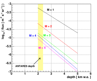
Figure 6.3: Vertical flux of muon bundles for different muon multiplicities $M$, after [Mar05a].

6.2 Atmospheric Neutrinos

Atmospheric neutrinos are produced when high-energy cosmic particles interact in the atmosphere of the Earth and produce charged mesons, which generate neutrinos in their decay. Due to the nature of the meson decay chains (see equation (2.1) in Section 2.3.2), the flux of atmospheric muon neutrinos is about twice as high as that of electron neutrinos, and it also extends to higher energies. Below a meson energy of about 500 TeV, the neutrino production is dominated by the decay of pions and kaons. This is called the conventional atmospheric neutrino flux. Above this energy, the lifetimes of the light mesons become large enough to allow them to interact before they can decay. Short-lived charm particles are the dominant source of atmospheric neutrino production at these higher energies; neutrinos produced in that way are called prompt atmospheric neutrinos.
The atmospheric neutrino flux as a function of the neutrino energy is shown in Figure 3.10 (Section 3.3.4). The marked areas in that plot show flux limits for $\nu_{\mu}$ (upper two lines) and $\nu_{e}$ (lower two lines) for different incident angles, as calculated by the Bartol group [Agr96] (conventional flux) and Naumov [Nau01] (prompt neutrinos), using the recombination quark-parton model (RQPM) [Bug98]. It should be noted that there exist several different models and predictions both for the conventional and the prompt neutrino flux; authors often cited for the conventional flux besides the one mentioned above are [Hon95] and [Vol80]. While the differences between the conventional models are up to $\sim 40\%$ at TeV energies [Mon01], the models for prompt neutrinos can differ more than one order of magnitude [Cos01] due to the lack of high-energy measurements of charm production cross sections in hadron-nucleus collisions.
A priori, atmospheric neutrinos are an irreduceable background in the detector; for the diffuse neutrino flux, one can differentiate between cosmic and atmospheric neutrinos by detecting the cosmic neutrinos as an excess of events in the energy spectrum of the atmospheric neutrinos. The diffuse cosmic neutrino flux is expected to exceed the atmospheric neutrino flux above some 10 – 100 TeV. Searching for individual sources, the usage of a small search window ($\lesssim 1^{\circ}\times 1^{\circ}$) reduces the background from atmospheric neutrinos significantly. On the other hand, the detection of atmospheric neutrinos is an important tool for the calibration of the detector and the fine-tuning of the event classification and reconstruction.

6.3 Optical Noise in the Deep Sea

The Baseline Rate

The noise rate in the deep sea can be divided into two components: the baseline and the bursts. The baseline is a slowly varying rate in each photomultiplier. It is produced partly by the radioactivity of the ⁴⁰K contained in the salt water, which produces a constant noise of $\sim 40$ kHz for the 10” photomultipliers used in ANTARES, and partly by the bioluminescence of micro-organisms which varies with the environmental parameters, like deep-sea current or weather conditions on the surface. This background causes mainly single, uncorrelated photon signals in individual photomultipliers, so that it can be removed to a large extent by a software filter (see Section 6.4).
The baseline rate is defined as the mean of a Gaussian which is fitted to the counting rate distribution measured in a period of 5 minutes [Esc05]. The ANTARES test strings PSL and MILOM (see Section 4.5) have observed baseline rates between 40 and almost 200 kHz; the long-term average is about 60–70 kHz. The baseline rate for a period of 3 days is shown in Figure 6.4, in the upper graph. It should be noted that also the photomultipliers themselves contribute to the baseline by their internal noise; this contribution is about 3 kHz [Esc05].

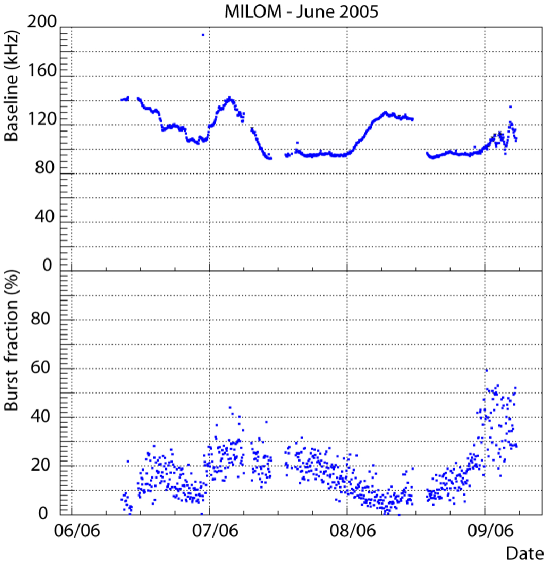
Figure 6.4: Baseline rate and burst fraction as measured by the MILOM between June 6th and 9th, 2005. From [ANT05b].

Bursts

Bursts are caused by all kinds of multi-cellular organisms which emit light: Fluorescent squids, crustaceans or fish. Contrary to the baseline rate, burst signals are very bright flashes lasting up to a few seconds, which cause counting rates up to several MHz in the nearby photomultipliers, but are aperiodic and localised, so that they do not affect the whole detector. The affected photomultipliers, however, have to be excluded from data taking during the burst.
The burst fraction in the optical background is defined as the fraction of time in a 5-minute window during which the counting rate in the photomultiplier exceeds the baseline by more than 20% [Esc05]. As for the baseline, the burst fraction also varies with time; there are periods where it is almost zero, whereas during other periods it rises to more than 40%. There is no direct correlation between a high baseline rate and a high burst fraction. An example for the burst fraction measured by the MILOM during a 3 day period is shown in the lower graph of Figure 6.4.
Figure 6.5 shows the counting rate of one photomultiplier of the PSL, in a 5-minute window. In this example the baseline rate is about 70 kHz, and a number of smaller bursts occur in irregular intervals.

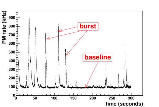
Figure 6.5: Photomultiplier counting rate within a 5-minute time window, as measured with the PSL. One can clearly distinguish the baseline at about 80 kHz and the bursts. The figure was taken from [Esc05] and slightly modified.

6.4 Suppression of Optical Background

The optical noise which causes the baseline rate can be suppressed by using the fact that the hits caused by this background are randomly distributed and uncorrelated. To prevent noise contamination of an event sample, the optical background must be filtered out before the reconstruction (contrary to atmospheric muon background which is removed by quality cuts after the reconstruction). This filtering is done for every single hit of an event by checking its correlation with the other hits. If a hit does not fulfill the filtering conditions listed in the following sections, it will be removed from the event. The first two conditions are taken from the ANTARES Software Trigger [Ren04] where they are used as trigger conditions to determine whether a physics event has been observed in the detector and should be written to disk, whereas the third condition was developed in the context of this thesis.

6.4.1 Filter Conditions for a Signal Hit

Condition 1: Global Causality

Every hit must be causally connected to the largest hit of the event. As the optical background hits are usually single photon hits, the largest hit is considered not to be caused by noise. The difference between the arrival time $t_{i}$ of the considered hit and the arrival time $t_{0}$ of the largest hit in the event must fulfill the condition

$$|t_{i}-t_{0}|\overset{!}{<}d/v+\delta t,$$ (6.1)

where $d$ is the distance of the two photomultipliers that were hit, $v$ is the speed of light in water and $\delta t=100$ ns is an extra time window to account for time measurement inaccuracies and delays due to scattering of the light.

Condition 2: Local Coincidences or Large Amplitude

Every hit must either have an amplitude larger than the adjustable $A_{min}$, or be in local coincidence within $\Delta t=20$ ns to at least one other hit on the same storey. $A_{min}$ was set to 3 photoelectrons (pe) for this study.

Condition 3: Background Coincidence Suppression

To avoid accidental coincidences of two background hits, those hits which have passed Condition 2 because they are in coincidence with another hit (and not because of their large amplitude) must fulfill an additional condition: A second pair of coincident hits on the same string is required. If there are no other coincident hits on the same string, the single pair of coincident hits can still pass the filter condition if at least one of the hits has an amplitude larger than $A_{min,2}$. $A_{min,2}$ is set to 1.5 pe, smaller than $A_{min}$, because the hits which this condition is applied to have already passed the other two conditions and the background has therefore already been reduced.
Conditions 1 and 2 are used in a very similar way in the ANTARES Software Trigger as trigger conditions for physics events; they are further described in [Ren04]. ${A_{min}=3}$ pe of Condition 2 is above the default value of 2.5 used for the Software Trigger, as in general higher amplitudes for showers than for muon events are expected in the individual photomultipliers.
Condition 3 has been implemented additionally in the context of this thesis, in order to prevent accidental coincidences between two background hits on the same storey. These coincidences are not so rare, as one can see from the following consideration:
The $k$-fold coincidence rate $R_{k}$ of $n$ photomultipliers within a coincidence window $\Delta t$ and for a background rate $r$ measured by each photomultiplier, is [Bla99]

$$R_{k}=\frac{n!}{(n-k)!}\cdot r^{2}\cdot\Delta t,$$ (6.2)

where $\frac{n!}{(n-k)!}=k!\begin{pmatrix}n\\ k\end{pmatrix}$ is the number of ordered sequences of $k$ samples taken from a total of $n$ samples, without repetition. For $n=3$ and $k=2$ (coincidence in two out of three photomultipliers on the same storey), and for $r=60$ kHz and $\Delta t=20$ ns, ${R_{k=2}=432}$ s^-1. The number of coincidences $N$ in the whole detector (300 storeys), for a typical event duration $T=2000$ ns, then becomes

$$N=300\cdot R_{k=2}\cdot T=0.26,$$ (6.3)

approximately one background coincidence in every four events. The number of coincidences grows quadratically with increasing background rate.
Only hits of an event which have passed all the conditions are used. These hits are required to be distributed on at least 3 different strings to generate a sufficiently large lever-arm for the reconstruction algorithm. If this is not the case, the event is discarded.

6.4.2 Event-wise Efficiency and Purity

One can define an event-wise efficiency and purity for the filtered events. The efficiency is the ratio of the number of events which have passed the filter conditions to the original number of events. The purity is the ratio of the number of good events which have passed the filter to the total number of events which have passed the filter. Here, good events are defined as events that have passed the filter purely because of signal hits. Therefore, as an estimate for the purity we consider the number of events of a background-free sample which have passed the filter, divided by the number of events of a background-contaminated sample which have passed the filter.
Figure 6.6 shows the efficiency and purity for event sample A (see appendix A.5), a sample of NC events with interactions within the instrumented volume and neutrino energies between 100 GeV and 100 PeV, for different rates of optical background per photomultiplier. For shower energies above 25 TeV the efficiency is practically 100%, whereas for energies smaller than 10 TeV it decreases strongly. At low energies, also many signal hits are cut away by the filter conditions, so that events fail to pass the filter; one can also see that the efficiency in these first three bins increases for higher background rates, which means that some of the background hits contribute to the coincidences and make the event pass the filter. This also shows up in the purity plot: For the lowest energy bin, the purity for the highest background rate of 140 kHz per photomultiplier is 0.65, so that 35% of the events are background-contaminated.
One can conclude that above 10 TeV, the background filter works well.

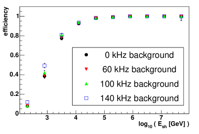
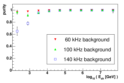
Figure 6.6: Efficiency (left) and purity (right) of the filter conditions described in the text, over shower energy, for event sample A. The error bars are merely statistical, and for most energy bins they are smaller than the points themselves. The calculation of these statistical errors is described separately in Appendix C.1.

6.4.3 Hit-wise Efficiency and Purity

The efficiencies and purities shown in the previous section state whether an event has passed the filter conditions or not; they do not indicate whether the hits remaining in the event after the filter contain only signal, or also a fraction of background. Note that a hit is generated by the photons, both from Cherenkov light and from optical noise, which arrive at a photomultiplier within 25 ns (see Section 4.3.1). We therefore define a signal hit as a hit with a background contribution to the amplitude below 1%. To examine the quality of the hits which pass the filter, the hit-wise efficiency and purity are introduced: The hit-wise efficiency is defined as the ratio of the number of signal hits after the filter to that before the filter. The hit-wise purity is defined as the ratio of the number of signal hits remaining after the filter to the total number of hits that are present after the filter. Note that a purity of e.g. 60% implies that in 40% of the hits a fraction $>1\%$ of the hit amplitude was caused by background. Efficiency and purity have been calculated on an event-by-event basis for a sample of $\sim 330$ events, selecting every 10th event of event sample A, both for 60 kHz and for 140 kHz optical background. The results are shown in figures 6.7 and 6.8. The numbers vary from event to event because the number of hits in an event does not only depend on the shower energy, but also on the position and direction of the shower with respect to the detector (note that the events used all had an interaction vertex inside the instrumented volume).
For the sample contaminated with 60 kHz noise, the hit-wise efficiency for events with a shower energy below 10 TeV is about 60%, increasing to about 90% for the higher energies. The purity for the 60 kHz sample is close to 100% up to $\sim 40$ TeV and decreases to about 70% for higher energies. This is due to the longer duration of the events, which causes a larger total number of background hits.
For the events with 140 kHz background, the results are very similar. There are, however, some additional events below 1 Tev, which have only passed the filter conditions because of the higher background rate.
It should be noted that the decrease in the purity for the highest energies (for both background rates shown) has no impact on the reconstructibility of these events, because the signal amplitudes at these energies are so high that the background only contributes a small fraction to the total hit amplitude. One can see this from Figure 6.9, where the amplitude fraction caused by signal hits with respect to the total amplitude measured in an event is calculated for 140 kHz background contamination, before the filter. The plots was retrieved without simulation of the detector electronics, i.e. the shown hits are the real photon signals, not the signals integrated over the ARS data taking time window (see Section 4.3.1). It is therefore possible to take into account the origin of the single photon signals, from Cherenkov radiation or optical background. One can see that for events above 100 TeV almost 100% of the amplitude is due to signal hits.

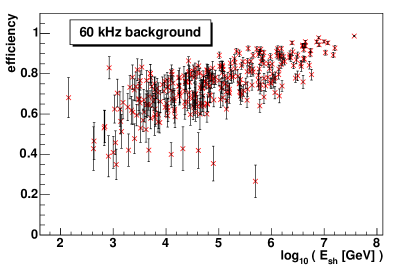
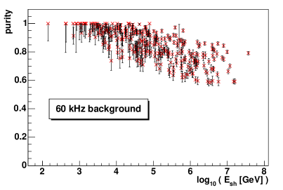
Figure 6.7: Hit-wise efficiency (left) and purity (right) of the filter conditions described in the text vs. the shower energy $E_{sh}$, for events with 60 kHz background per photomultiplier. Each cross stands for one event. Statistical errors calculated according to Appendix C.1 are also shown.

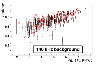
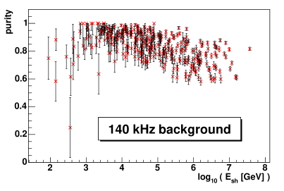
Figure 6.8: Hit-wise efficiency (left) and purity (right) of the filter conditions described in the text vs. the shower energy $E_{sh}$, for events with 140 kHz background per photomultiplier. Each cross stands for one event. Statistical errors calculated according to Appendix C.1 are also shown.

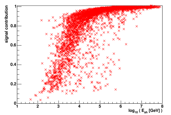
Figure 6.9: Contribution of signal hits to the total amplitude of an event as a function of the shower energy, for 140 kHz background, before the filter.

The studies show that the filter assures a satisfying suppression of the background above 10 TeV, while for lower energies the majority of events is discarded. The pattern matching algorithm for the shower reconstruction (see Chapter 8) yields best results above 10 TeV (see also Chapter 10, where the results for the shower reconstruction are presented). The reconstruction of low-energy events in the region below 10 TeV requires the use of other methods of background suppression, and different reconstruction algorithms, and is outside the scope of this thesis.

Chapter 7 Strategies for the Reconstruction of Individual Shower Parameters

This chapter addresses strategies for the separate reconstruction of individual parameters of a shower: the position, the direction of the shower axis and the shower energy. Some of the algorithms described here are part of the shower reconstruction package ShowerFitter which was created within the context of this thesis. Other algorithms have been developed to check the shower characteristics and are not intended for the use in a more sophisticated analysis.
Section 7.1 describes an algorithm for the reconstruction of the interaction vertex, needed as an auxiliary variable for the reconstruction of direction and energy. The interaction time is reconstructed in the same step but not used for further analysis.
In Section 7.2, strategies for the reconstruction of the shower direction are described. These algorithms are intended to provide a first estimate of the shower direction; the resolution which results from these algorithms is not good enough to qualify them for a precise physics analysis. They can, however, be used to check the consistency of the final fit.
Section 7.3 describes a method to reconstruct the energy of a shower, if its direction and the interaction vertex are known. This method is not used in the final reconstruction, but it provides a good consistency check for the combined reconstruction of direction and energy.
It should be noted that within the context of this work, the shower direction is considered to be identical with the neutrino direction, which is a very good approximation within the precision of a few degrees that can be reached in the direction reconstruction (see Section 5.3.3). For the angular resolution, the reconstructed shower direction will therefore be directly compared to the MC neutrino direction.

7.1 Reconstruction of the Interaction Vertex

7.1.1 Method

The reconstruction of the interaction vertex is based on the simple assumption that a shower is a point-like object, as compared to the granularity of the detector. Therefore, all the light which is produced in a shower is assumed to be emitted from one point. The point which is reconstructed under this assumption is in fact not equivalent to the interaction vertex of the neutrino, but should rather be denoted as OM-centre-of-gravity $\vec{r}_{\text{CG}}$ (the centre-of-gravity of all Optical Modules (OMs) which have been hit in the event). To calculate $\vec{r}_{\text{CG}}$, the point of photon emission is calculated from the time and position of all hits, but neglecting the hit amplitudes. To retrieve the true centre-of-gravity of a shower $\vec{r}_{\text{CGA}}$, as defined in Section 5.3, the amplitudes of the hits are also taken into account. The relation between these two positions will be discussed below.
Under the assumption of a point-like light source, the photon emission point can be reconstructed via a simple triangulation. For an event with hits in $N$ OMs with space-time coordinates $\vec{x}_{i}=(x_{i},y_{i},z_{i},t_{i})$ ($i=1,...,N$) and an unknown space-time position of the shower $\vec{x}=(x,y,z,t)$, the distance $d_{i}$ between $\vec{x}$ and $\vec{x}_{i}$ can be written as

$$d_{i}=\sqrt{(x-x_{i})^{2}+(y-y_{i})^{2}+(z-z_{i})^{2}}=c/n\cdot(t-t_{i})$$ (7.1)

where $c/n$ is the velocity of light in water with the refraction index $n$. The situation is shown schematically for $N=5$ in Figure 7.1. Note that in the ANTARES coordinate system the spacial point (0,0,0) lies in the centre of the detector, with the $x$ axis pointing towards East, the $y$ axis towards North and the $z$ axis vertically upward (see Figure 4.5).

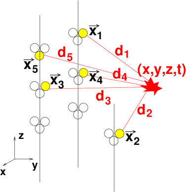
Figure 7.1: Schematic view of the geometric situation for the reconstruction of the shower position $(x,y,z)$ and interaction time $t$.

Equation (7.1) yields a system of $N$ equations which are quadratic in the unknown $\vec{x}$. By pairwise subtraction of these equations, the quadratic terms of the components of $\vec{x}$ cancel out and one is left with an $(N-1)$–dimensional linear equation system of the form

$$x_{i+1}^{2}-x_{i}^{2}+y_{i+1}^{2}-y_{i}^{2}+z_{i+1}^{2}-z_{i}^{2}-(c/n)^{2}t_{i+1}^{2}+(c/n)^{2}t_{i}^{2}$$

$$= 2x\cdot(x_{i+1}-x_{i})+2y\cdot(y_{i+1}-y_{i})+2z\cdot(z_{i+1}-z_{i})-2(c/n)^{2}t\cdot(t_{i+1}-t_{i}).$$ (7.2)

This equation system can be written as

$$A\cdot\vec{x}=\vec{b},$$ (7.3)

where $A$ is a $(N-1)\times 4$ matrix with the components

$$a_{j1} =2\,(x_{j+1}-x_{j})$$

$$a_{j2} =2\,(y_{j+1}-y_{j})$$

$$a_{j3} =2\,(z_{j+1}-z_{j})$$

$$a_{j4} =-2\,(c/n)^{2}(t_{j+1}-t_{j}),$$ (7.4)

and $\vec{b}$ is a vector with the components

$$b_{j}=x_{j+1}^{2}-x_{j}^{2}+y_{j+1}^{2}-y_{j}^{2}+z_{j+1}^{2}-z_{j}^{2}-(c/n)^{2}\cdot(t_{j+1}^{2}-t_{j}^{2}),$$ (7.5)

with $j=1,...,N-1$.
The system (7.3) will normally not have an exact solution; a residual vector ${\vec{r}=A\vec{x}-\vec{b}}$, ${\vec{r}\neq\vec{0}}$ will remain. The best solution $\vec{x}$ of the equation system is given by the condition

$$\sum_{j}r_{j}^{2}=\vec{r}^{T}\vec{r}=(A\vec{x}-\vec{b})^{T}(A\vec{x}-\vec{b})=\text{minimal}.$$ (7.6)

Differentiating equation (7.6) by $\vec{x}$ results in

$$2A^{T}A\vec{x}-2A^{T}\vec{b}=0\leadsto\vec{x}=(A^{T}A)^{-1}A^{T}\vec{b}.$$ (7.7)

This solution for $\vec{x}$ is calculated analytically. There are four unknowns in the $(N-1)$–dimensional equation system (7.3), so $N$ must be at least 5 to constrain $\vec{x}$ unambiguously. As a further condition, it is required that hits occur on at least 3 different strings. This is necessary to ensure that the equation system (7.3) is solvable for all geometries. To ensure numerical stability, the pairwise subtractions in equation (7.1.1) are arranged such that they preferentially involve hits from different strings.

7.1.2 Calculation of the Centre-of-Gravity of a Shower

As mentioned above, the centre-of-gravity of a shower $\vec{r}_{\text{CGA}}$, as introduced in Section 5.3, is defined as the point of photon emission calculated from the amplitude-weighted positions and times of the hits. To calculate $\vec{r}_{\text{CGA}}$ from the physics information that is available after the detector simulation, one has to follow the algorithm introduced in the last section, but the contributions of the respective OMs have to be weighted according to the hit amplitude that the OMs have measured.
However, the resolution achieved when calculating $\vec{r}_{\text{CGA}}$ is not better than the resolution achieved for the calculation of the OM-centre-of-gravity $\vec{r}_{\text{CG}}$. In the combined reconstruction of direction and energy, for which the shower position is needed as an auxiliary parameter, it makes no difference whether the interaction vertex, $\vec{r}_{\text{CG}}$ or $\vec{r}_{\text{CGA}}$ is used as shower position, as long as the same variable is used consistently throughout the reconstruction. It was therefore chosen to use $\vec{r}_{\text{CG}}$ throughout this thesis.

7.1.3 Results for Events without Background

The distance between the interaction vertex and $\vec{r}_{\text{CG}}$ is larger than the distance between the interaction vertex and $\vec{r}_{\text{CGA}}$. This can be seen in Figure 7.2 for event sample A (see Appendix A.5), without optical background and without the usage of the filter for background suppression (see Section 6.4): On the left, the total distance between $\vec{r}_{\text{CG}}$ and the true interaction vertex is shown. The average offset is $\sim 5.4$ m. On the right, the correlation between that distance and the shower energy is shown. A linear function in $\log_{10}E$ (shown in red) has been fitted to the data within the region marked by the endpoints of the line. The numerical values are:

$$\Delta r(E)/\textrm{m}=2.8+0.48\cdot\log_{10}(E/\textrm{GeV}),$$ (7.8)

with $\Delta r(E)=|$$\vec{r}_{\text{CG}}$$-\vec{r}_{\text{MC}}|$, the distance between $\vec{r}_{\text{CG}}$ and the MC interaction vertex. The green line marks the distance between $\vec{r}_{\text{CGA}}$ and the MC interaction vertex, equation (5.4) (cf. Section 5.3). The distance between the interaction vertex and $\vec{r}_{\text{CG}}$ grows more steeply with increasing energy than the distance between the interaction vertex and $\vec{r}_{\text{CGA}}$. This is possibly due to the fact that for increasing energy, a larger amount of Cherenkov light is radiated in a transverse direction (see Figure 5.9), and therefore, the hit amplitude in OMs positioned at larger polar angles with respect to the shower axis increases. This is not taken into account in the calculation of $\vec{r}_{\text{CG}}$, as all OMs are treated in the same way and information regarding the hit amplitude is not used, and therefore the OMs in forward direction have too large an impact on the reconstructed position.
$\vec{r}_{\text{CG}}$and $\vec{r}_{\text{CGA}}$are at the same position at $\sim 40$ TeV, and there is a discrepancy of $\sim 1.5$ m for the highest energies studied.

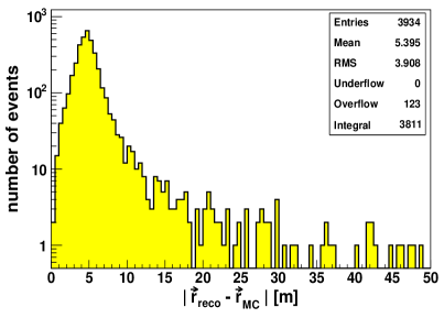
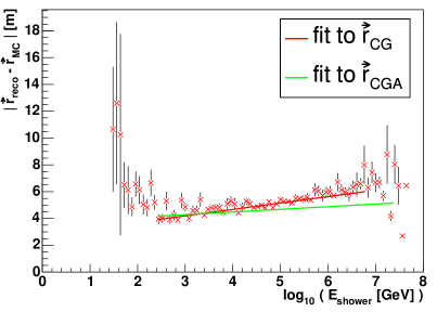
Figure 7.2: Left: Total distance between reconstructed position and Monte Carlo (MC) vertex. Right: Profile of the distance, plotted as a function of the MC shower energy. The green line refers to equation (5.4) from Section 5.3, the red line is a fit to the data shown; the endpoints of the line mark the range of the fit.

Figure 7.3 shows the results of the reconstruction of $\vec{r}_{\text{CGA}}$ for the individual spacial coordinates and the interaction time. The plots show as red lines the resolution of the three spacial coordinates $x,y,z$ after the reconstruction.
As mentioned above, $\vec{r}_{\text{CG}}$ is a suitable auxiliary variable for the reconstruction of direction and energy. If a knowledge of the interaction vertex is desired, its coordinates can be calculated from $\vec{r}_{\text{CG}}$ following equation (7.8), if direction and energy are known (from reconstruction or MC). The results of this calculation, using MC values, is shown as yellow filled histograms in the same figure. The individual coordinates are now in good agreement with the MC values. The resolution reaches values between 3.5 m and 4.5 m.
The slight trend to positive values in the $z$ coordinate, both before and after the correction towards the interaction vertex, is caused by the non-isotropic angular acceptance of the OMs which was not corrected for here. As the OMs are orientated looking downward at a 45^∘ angle (see Section 4.2), they are less sensitive for light coming from above than for light coming from below; however, the position reconstruction assumes an isotropic light detection efficiency, which leads to a slight overestimate of the $z$ coordinate.
Figure 7.3 also shows the resolution of the reconstruction of the interaction time, again before (red lines), and after the correction towards the interaction vertex (yellow areas). The offset $\Delta t\approx 20$ ns before the correction corresponds to the distance $\Delta r$ between the interaction vertex and $\vec{r}_{\text{CG}}$ and is corrected accordingly, assuming that the particle is travelling with the speed of light. For this correction, again the MC values of energy and direction were used. The mean of the time distribution is closer to zero after the correction, though still slightly shifted to times reconstructed too large.
It can therefore be concluded that it is possible to reconstruct $\vec{r}_{\text{CG}}$ and the interaction vertex of the shower with a resolution of a few metres by this method. As mentioned above, the interaction vertex is not needed for the final reconstruction of direction and energy, as $\vec{r}_{\text{CG}}$ is the reconstructed position which is used throughout all following reconstruction steps of the ShowerFitter (see following chapter).
The reconstructed position is an important parameter for the reconstruction of direction and energy, as the fit for direction and energy is likely to fail, if a wrong position is used (see Section 8.2.3).

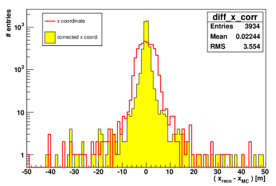
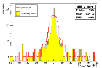
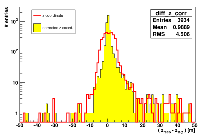
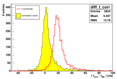
Figure 7.3: Results of the reconstruction of the interaction point. Shown are the differences between the reconstructed spacial coordinates $x,y,z$ and those from the MC, and the difference between the reconstructed and the MC interaction time. The red line shows the results for the reconstruction of $\vec{r}_{\text{CG}}$, the yellow filled histograms those after correcting $\vec{r}_{\text{CG}}$ towards the interaction vertex, using equation (7.8).

7.1.4 Results for Events with Optical Background

Figures 7.2 and 7.3 are the results of the position reconstruction for a background-free event sample. However, at the ANTARES site, signal events always contain optical noise from the deep sea (see Section 6.3). A filter strategy to suppress this background has been described in Section 6.4. The strategy is based on the distinction between physics hits caused by Cherenkov radiation and optical noise hits. However, it is unavoidable that some of the physics hits are also cut away in the filter or that some background hits remain in the sample. Therefore, the results of the position reconstruction will be slightly different for events with background and using the filter conditions.
Figure 7.4 shows the results of the position reconstruction for the same data sample as used above, with neutrino energies between 100 GeV and 100 PeV, but with 60 kHz optical noise added per OM. A fit to the data is shown in black, given by

$$|\vec{r}_{\text{CG}}-\vec{r}_{\text{MC}}|/\textrm{m}=\Delta r(E)/\textrm{m}=3.9+0.36\cdot\log_{10}(E/\textrm{GeV}).$$ (7.9)

The left plot indicates that the resolution has deteriorated, and also that some 660 events, mainly with very small shower energies below 100 GeV (see Figure 7.5), are missing in the event sample because they did not pass the filter conditions. From Figure 7.5 it can be seen that events with a shower energy above $\sim 40$ TeV show very similar results with and without background, which is due to the larger overall number of hits in these events. For events with a lower energy, on the other hand, the offset between the reconstructed and the true position is slightly larger for the sample with than for the sample without background.

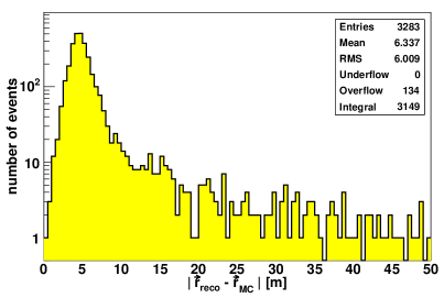
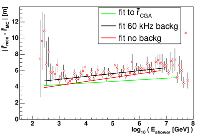
Figure 7.4: Left: Total distance between reconstructed and MC vertex, for an event sample with 60 kHz background. Right: Profile of the distance, plotted as a function of the MC shower energy. The green line again refers to equation (5.4) from Section 5.3, the red line is the fit to the background-free data shown in Figure 7.2, and the black line is a fit to the data shown in this figure.

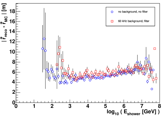
Figure 7.5: Comparison of the results of the position reconstruction for background-free events (blue circles) and the results for the same events with 60 kHz background added and after the filter conditions (red squares).

7.2 Reconstruction of the Shower Direction

7.2.1 Method 1: Using the Cherenkov Angle

An isolated charged particle (e.g. a muon) traversing the detector medium produces Cherenkov light on a cone along its track. The opening angle of this cone depends on the refraction index of the medium and is around $42.2^{\circ}$ at the ANTARES site (see Section 4.4.2). This is also true for the individual charged particles in a shower; however, with respect to the shower axis, the angular distribution of the photons is rather broad, with a peak around the Cherenkov angle (see Section 5.3).
To get a rough estimate of the shower direction, e.g. as a starting value for a later fit, one can assume that all photons are produced on a Cherenkov cone under a fixed angle with respect to the shower axis. One can then develop an algorithm to calculate the shower direction from the position of the hits. This algorithm is very similar to the one described in Section 7.1. For shower reconstruction in ANTARES it has first been described in [Nau03]. Its advantage is that it does not need the reconstructed interaction point as input information.
Consider Figure 7.6, where $\vec{x}=(x,y,z)$ represents the position vector of the interaction and $\vec{v}=(v_{x},v_{y},v_{z})$ the direction vector of the shower. Here, the direction of the shower is approximated by the direction of the neutrino (see Section 5.3).

Figure 7.6: Schematic view of the geometric situation for the reconstruction of the direction. $\vec{v}$ is the direction of the shower, $X$ and $X_{i}$ mark the position of the shower and OM_i, respectively, and $\vartheta_{C}$ is the Cherenkov angle, $42.2^{\circ}$.

A photon emitted under the Cherenkov angle $\vartheta_{C}$ hits OM_i, which has the coordinates $\vec{x}_{i}=(x_{i},y_{i},z_{i})$. The vector $\vec{d}_{i}$ connecting the points $X$ and $X_{i}$ is then defined by ${\vec{d}_{i}=(x_{i}-x,y_{i}-y,z_{i}-z)}$, with

$$\cos\vartheta_{C}=\frac{\vec{v}\cdot\vec{d}_{i}}{|\vec{v}|\cdot|\vec{d}_{i}|}$$ (7.10)

for all hits $i$. The norm of $\vec{d}_{i}$ can be written using the speed of light and the travel time: $|\vec{d_{i}}|=(c/n)(t_{i}-t)$. Suppose $|\vec{v}|\equiv 1$; then equation (7.10) can be rewritten as

$$\cos\vartheta_{C}\cdot(c/n)\cdot(t_{i}-t)=v_{x}\cdot(x_{i}-x)+v_{y}\cdot(y_{i}-y)+v_{z}\cdot(z_{i}-z)$$

for all hits $i$ in the event. Again one can subtract these equations pairwise, thus eliminating the contributions of $\vec{x}$. For $N$ hits one obtains $(N-1)$ equations of the form

$$\cos\vartheta_{C}\cdot(c/n)\cdot(t_{i}-t_{i+1})=v_{x}\cdot(x_{i}-x_{i+1})+v_{y}\cdot(y_{i}-y_{i+1})+v_{z}\cdot(z_{i}-z_{i+1})$$

where $v_{x},v_{y}$ and $v_{z}$ are the unknown quantities. This system of equations can be solved as described in Section 7.1.
This algorithm yields a rough estimate of the shower direction, as shown in Figure 7.7 for event sample A, without background. The resolution is about 36^∘ in zenith angle $\theta$ and 79^∘ in azimuth angle $\phi$. In $\theta$, there is a systematic shift towards small angles which is due to the fact that downgoing events ($\theta>90^{\circ}$) are often misreconstructed as upgoing. This is illustrated in Figure 7.9, where the reconstructed (in green) and the MC values (bold line) of $\theta$ are plotted for each event. While the MC distribution is flat in $\cos\theta$, the reconstructed one shows a clear trend towards smaller values of $\theta$ and therefore tends to reconstruct downgoing events as upgoing. The effect can be explained as schematically shown in Figure 7.9: One side (marked as a blue, dotted line) of the Cherenkov cone cannot be detected because the light hits the OM at an angle where the OM’s angular acceptance is zero. With the information from only one side of the cone, the direction of the shower might as well be the vector marked $\vec{v}^{\prime}$ in the plot. In this case, the reconstructed direction is $2\vartheta_{C}$ off the real direction and is upgoing instead of downgoing. In a real event with hits in more than two OMs, the effect of the missing information is less prominent, and the shift in $\theta$ is about $-35^{\circ}$ on average.
The result of this method depends also on the shower energy. This is demonstrated in Figure 7.10, where the differences between the reconstructed and the MC angles, as shown in Figure 7.7, are plotted versus the MC shower energy. Especially for $\phi$, the resolution deteriorates very strongly for increasing shower energies. This deterioration can be understood from the fact that the distribution of the photon radiation angle with respect to the shower axis becomes broader and broader for higher shower energies (cf. Figure 5.9).

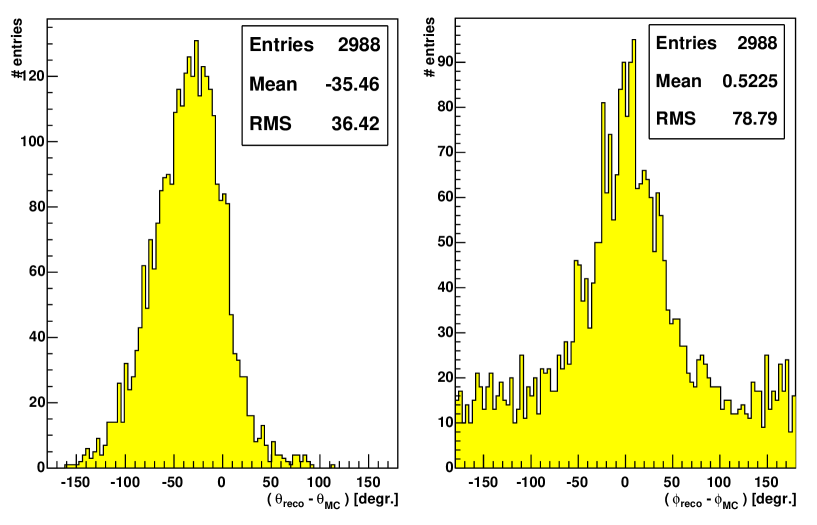
Figure 7.7: Results of the reconstruction of the direction, using the Cherenkov cone condition, for the zenith angle $\theta$ and the azimuth angle $\phi$. Shown are the differences between the reconstructed angles and the true MC angles.

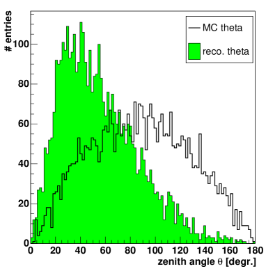
Figure 7.8: MC and reconstructed zenith angle $\theta$. It is clearly visible how the reconstruction tends to misreconstruct downgoing events ($\theta>90^{\circ}$) as upgoing.

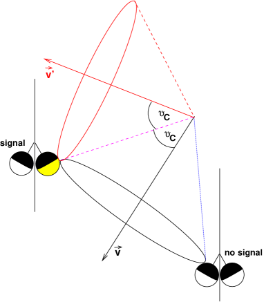
Figure 7.9: Schematic view of a possible misreconstruction: Instead of the true direction $\vec{v}$, the reconstruction produces $\vec{v}^{\prime}$ as a result, due to the unfavourable angle with respect to the OM orientation.

7.2.2 Method 2: Amplitude Ratio

As shown in the previous subsection, the reconstruction of the shower direction with the Cherenkov angle method is not always successful. The knowledge of the neutrino orientation, i.e. whether a neutrino is upgoing or downgoing, is, however, a significant quantity in the reconstruction. Most importantly, it has to be excluded that the event was caused by a downgoing atmospheric muon imitating a shower (see Section 6.1), instead of an upgoing neutrino.
Therefore, a method was developed to be able to quickly distinguish between upgoing and downgoing events. The algorithm is simple: The detector is divided into two regions by placing a horizontal plane, the so-called $Z$-plane, at the $z$-coordinate of the interaction vertex. The assumption is then that for upgoing events, the largest part of the emitted light is measured in OMs which are positioned above the $Z$-plane, while for downgoing events, a larger fraction is measured below the $Z$-plane. A schematic view of the geometric principle is shown in Figure 7.11.
To discriminate between upgoing and downgoing events, the ratio $r_{pe}$ of the amplitudes measured in the two regions, i.e. of the total number of photo-electrons in OMs above the $Z$-plane, $n_{pe}^{>}$, and below the $Z$-plane, $n_{pe}^{<}$, is calculated:

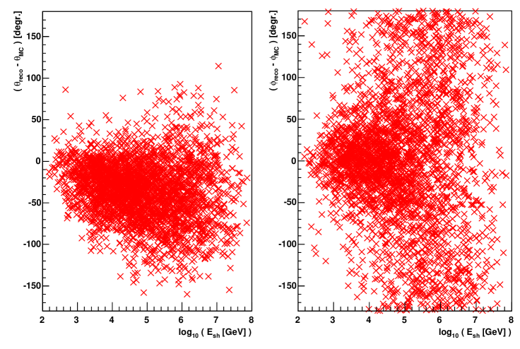
Figure 7.10: Resolution of the zenith angle $\theta$ (left) and the azimuth angle $\phi$ (right) as shown in Figure 7.7, plotted vs. the MC shower energy.

$$r_{pe}=\frac{n_{pe}^{>}}{n_{pe}^{<}}.$$ (7.11)

To avoid edge effects, the regions inside which $n_{pe}^{>}$ and $n_{pe}^{<}$ are evaluated are chosen symmetrically, i.e. the number of storeys used for the calculation is the same for both sides of the $Z$-plane and defined by the minimum number of storeys between the $Z$-plane and the detector top or bottom. By this method, the probability that $r_{pe}$ is affected by edge effects is reduced. Note that $r_{pe}$ can only be calculated if the event occurs well inside the detector, such that $n_{pe}^{<}\neq 0$.
$r_{pe}$ as calculated for MC events from event sample A without background is shown in Figure 7.12 on the left hand side. As expected, $r_{pe}$ is much smaller for downgoing than for upgoing events. By applying a cut on $r_{pe}$, events are classified as downgoing or upgoing, respectively. In the example shown here, the cut was applied at $r_{pe}=3.3$. 88.1% of the upgoing events are above that value, so that the probability to misinterpret an upgoing neutrino as downgoing is 11.9%; on the other hand, 80.7% of the downgoing events have a ratio smaller than 3.3, so that the probability to misinterpret a downgoing neutrino as upgoing is 19.3%.

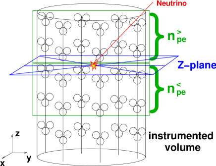
Figure 7.11: Geometric principle of the amplitude ratio method: The instrumented volume is symmetrically divided into two parts by a horizontal plane through the $z$-coordinate of the interaction vertex.

The right hand side of Figure 7.12 shows the improvement which is possible if this method is combined with the one from Section 7.2.1: The red histogram shows the equivalent distribution as in Figure 7.7 (left). The reconstructed values of $\theta$ were then corrected by using $r_{pe}$; if the orientation did not agree with the reconstructed $\theta$, $\theta$ was shifted to $\pi-\theta$. The comparison of the reconstructed and the MC direction after this correction is shown on the right hand side of Figure 7.12 in yellow. Both the mean and the RMS of the distribution are improved by the correction. The number of events shown in Figure 7.12 is smaller than in Figure 7.7, as the events with undetermined $r_{pe}$ (due to $n_{pe}^{<}=0$) have been removed from the sample.

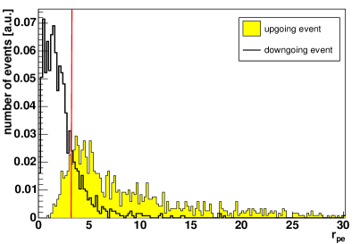
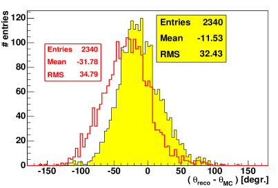
Figure 7.12: Left: Ratio of pe above and below the shower position, for upgoing and downgoing events; both histograms have been normalised to 1. The red line marks the cut proposed at a ratio of 3.3. Right: Distribution of the difference between the reconstructed and the MC $\theta$ angles, before the amplitude ratio correction (red lines) and afterwards (yellow histogram).

7.3 Energy Reconstruction

The algorithm for the reconstruction of the shower energy which is described in this section uses the fact that the total hit amplitude, i.e. the sum of the amplitudes of all hits in an event, corrected according to distance and angle of each hit with respect to the shower, is correlated to the shower energy. The method described here is not used in the final energy determination, but is useful for consistency checks or for the analysis of data with known shower direction and interaction vertex. It uses the simplified assumption that all photons are emitted from one point, $\vec{r}_{\text{CG}}$ (see Section 7.1), marked $X$ in Figure 7.13, and under a fixed polar angle $\vartheta_{C}$ with respect to the shower axis, i.e. along a cone (see Figure 7.13). $\vartheta_{C}$ is defined as:

$$\cos\vartheta_{C}=\frac{\vec{d_{i}}\cdot\vec{v}}{|\vec{d_{i}}|\cdot|\vec{v}|}$$ (7.12)

Assuming that the photons are emitted isotropically in the azimuthal angle $\varphi$, the photon density (in units of length^-1) at a distance $d=|\vec{d}|$ from $\vec{r}_{\text{CG}}$ is proportional to the inverse of the circumference of the cone, and thus proportional to $1/R=1/(d\cdot\sin(\vartheta_{C}))$ (see Figure 7.13). The measured amplitude $a_{i}$ in OM $i$ can therefore be regarded as the photon density times a unit segment of the circle, $a_{i,0}=\rho_{i}\cdot 2\pi R_{0}$; the total number of photons on the circle is then $a_{i}=\rho_{i}\cdot 2\pi R_{i}=a_{i,0}\cdot R_{i}/R_{0}$. The attenuation in water, $\exp(-d/\tau)$, is also taken into account; as scattering is not fully simulated in the light propagation software, the attenuation length $\tau$ is set to 55 m, which corresponds to the absorption length at 475 nm, the wavelength of maximum absorption at the ANTARES site (see Section 4.4.1). Thus, the corrected number of photons $a_{i}^{corr}$ emitted along the cone hitting OM $i$ is $a_{i}^{corr}=a_{i}\exp(d_{i}/\tau)$. The total number of photons $\mathcal{A}$ in an event with $N$ hits is therefore

$$\mathcal{A}=\sum_{i=1}^{N}a_{i}^{corr}=\sum_{i=1}^{N}a_{i,0}\cdot\frac{R_{i}}{R_{0}}\cdot\exp(d_{i}/\tau).$$ (7.13)

Figure 7.13: Schematic view of the geometric situation for the reconstruction of the energy: $\vec{v}$ is the direction of the shower axis, while $\vec{d_{i}}$ is the direction of the photon hitting OM $i$.

For event sample A, without optical background, $\mathcal{A}$ was calculated using the MC direction and $\vec{r}_{\text{CG}}$ calculated according to equation (7.8), using MC values. The distribution of $\mathcal{A}$ versus the MC shower energy $E_{sh}$ is shown in Figure 7.14 on the left hand side.

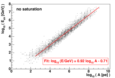
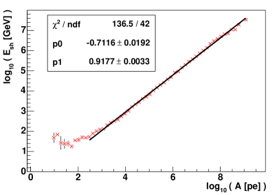
Figure 7.14: Left: Shower energy $E_{sh}$ in GeV vs. total corrected amplitude $\mathcal{A}$ per event. The linear function which has been fitted to the distribution is also shown. Right: Profile of the distribution shown on the left, and fit.

To find a fit curve to this distribution, the profile of the MC shower energy $E_{sh}$ with respect to $\mathcal{A}$ has been considered, and a polynomial has been fit to that profile, as shown on the right hand side of Figure 7.14. This yields the following relation between averaged total amplitude and shower energy:

$$\log_{10}(E_{sh}/{\textrm{GeV}})=0.92\cdot\log_{10}\mathcal{A}-0.71.$$ (7.14)

Something which has not been taken into account for the calculation of the total amplitude $\mathcal{A}$ is the fact that the photomultiplier electronics saturate at a certain amplitude, depending on the data taking mode (see Section 4.3.1). To study the effect of saturation on the energy reconstruction, two values for saturation, 200 pe (equivalent to the WF mode) and 20 pe (equivalent to the SPE mode) have been studied in addition to the non-saturation case shown before. The resulting distributions are shown in Figure 7.15.

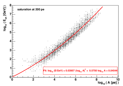
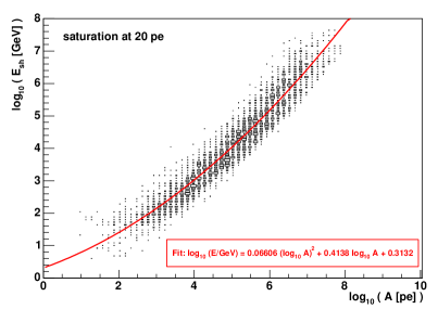
Figure 7.15: Shower energy $E_{sh}$ in GeV vs. total corrected amplitude $\mathcal{A}$ per event, for a saturation at 200 pe (left) and 20 pe (right). The polynomials which have been fitted to the distributions are also shown.

For the saturation at 200 pe, one finds the following parameterisation for the shower energy:

$$\log_{10}(E_{sh}/{\textrm{GeV}})=0.040\cdot(\log_{10}\mathcal{A})^{2}+0.58\cdot\log_{10}\mathcal{A}+0.045;$$ (7.15)

for the saturation at 20 pe, the parameterisation becomes

$$\log_{10}(E_{sh}/{\textrm{GeV}})=0.066\cdot(\log_{10}\mathcal{A})^{2}+0.41\cdot\log_{10}\mathcal{A}+0.31.$$ (7.16)

As this algorithm makes use of the shower position and direction, it can only be used if these two values are at least approximately known.
Results for this energy reconstruction method using the MC values for shower position and direction are shown in figures 7.16, 7.17 and 7.18 for no saturation, saturation at 200 pe, and saturation at 20 pe, respectively. All plots show distributions of the logarithmic difference of the reconstructed and the MC shower energy on the left hand side, and the logarithm of the reconstructed energy versus that of the MC shower energy on the right hand side. The ideal result of a complete agreement is marked by a diagonal line. No event or hit selection of any kind was used in this reconstruction, and the events were background-free.
The best results are obtained in case of no saturation. The overall resolution is $\sim 0.32$, which corresponds to a factor of $10^{0.32}\approx 2.1$ in energy. One can see on the right hand side of Figure 7.16 that the resolution remains approximately constant for all energies.
In the case of saturation at 200 pe, the WF mode, the resolution deteriorates slightly to $0.36$, corresponding to a factor of $10^{0.36}\approx 2.3$ in energy, and for saturation at 20 pe, the SPE mode, the resolution becomes $0.40$, which corresponds to $10^{0.40}\approx 2.5$. The deterioration is not surprising, since the relation between the measured amplitude and the shower energy is smeared by the saturation effects.
For this comparably simple method and keeping in mind the simplifications that have been used in describing the correlation between total amplitude and energy, these results are satisfying. The resolution is already in the same order of magnitude as the resolution achieved for the reconstructed muon energy in ANTARES [Rom03].

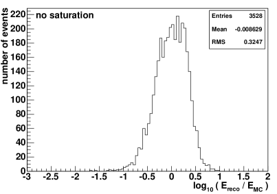
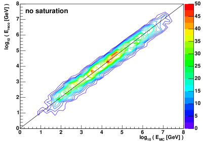
Figure 7.16: Results of the energy reconstruction using the corrected total amplitude, for the case of no saturation: Distribution of the logarithmic quotient of reconstructed and MC shower energy (left), and reconstructed versus MC shower energy as contour plot (right).

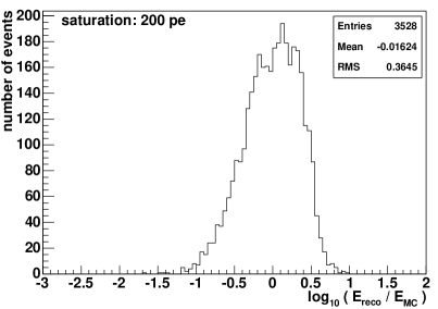
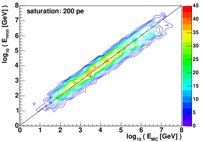
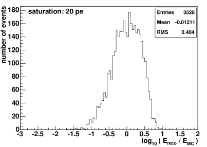
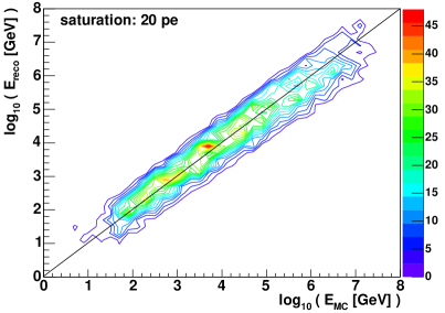
Figure 7.17: Results of the energy reconstruction using the corrected total amplitude, for the WF mode case, saturation at 200 pe: Distribution of the logarithmic quotient of reconstructed and MC shower energy (left), and reconstructed versus MC shower energy as contour plot (right).

Figure 7.18: Results of the energy reconstruction using the corrected total amplitude, for the SPE mode case, saturation at 20 pe: Distribution of the logarithmic quotient of reconstructed and MC shower energy (left), and reconstructed versus MC shower energy as contour plot (right).

Chapter 8 Combined Reconstruction of Shower Parameters using a Maximum Likelihood Fit

The major reconstruction package ShowerFitter, which was developed in the context of this thesis, reconstructs simultaneously the direction and energy of a neutrino-induced shower, using a maximum likelihood fit. This chapter describes the reconstruction algorithm applied, i.e. the matching between the measured and the calculated hit amplitudes in each Optical Module (OM).
In Section 8.1 the calculation of the hit amplitude in an OM is discussed, while Section 8.2 provides further details of the fit, like the determination of the initial parameter values, and a closer examination of the likelihood parameter space with examples for different event topologies.

8.1 Pattern Matching Algorithm

The reconstruction of a hadronic shower in a sparsely instrumented detector like ANTARES is a challenging task, due to fluctuations in the Cherenkov light emission between different showers, and the fact that most of the light is lost in the sparsely instrumented detector. It is therefore important that all relevant information available from the measurements is used. As a consequence, it is not only important for the reconstruction which OMs have been hit (or not hit), but also how large the hit amplitudes are.
The reconstruction strategy presented here is based on pattern matching: For an assumed shower direction and energy, what would be the expected hit amplitude in each OM? And how does this hit pattern compare to the actual measurement?
The variables which are to be determined are the shower direction, i.e. the azimuth angle $\phi$ and the zenith angle $\theta$, and the shower energy. As the pattern matching deals with hit amplitudes, and as the total hit amplitude of an event is directly correlated to the shower energy (see e.g. Figure 8.10), the total hit amplitude, in other words, number of (measured) photo-electrons will be used as third fit parameter. The conversion between the number of photo-electrons and the shower energy will be discussed at the end of this section.

8.1.1 Geometrical Situation, OM Efficiency and Attenuation

To correlate the shower direction with the measured hit amplitudes, some geometrical considerations are needed. The situation is explained schematically in Figure 8.2; the following notations are used:

• $\vec{v}$ = assumed direction of the shower

• $P$ = point from which a photon generating hit $i$ was emitted from the shower

• $Q_{i}$ = position of OM_i which has measured the corresponding hit $i$

• $\overrightarrow{PQ_{i}}$ = direction of the photon

• $\vartheta_{i}$ = angle between $\vec{v}$ and $\overrightarrow{PQ_{i}}$

• $\alpha_{i}$ = opening angle of OM_i, approximated as $\tan\alpha_{i}=R_{OM}/|\overrightarrow{PQ_{i}}|$, with the OM radius $R_{OM}=21.7$ cm

• $\vec{o}_{i}$ = orientation of OM_i

• $\gamma_{i}$ = angle between $\overrightarrow{PQ_{i}}$ and $\vec{o}_{i}$.

In order to obtain the total number of photo-electrons $N$ in the event from the hit amplitude $n_{i}$ in one OM, the relative angular efficiency $a_{i}(\gamma_{i})$ of the OM has to be taken into account. A parameterisation from the ANTARES software [Cas99b] has been used to describe the angular efficiency. The parameterised function $a_{i}$ is shown in Figure 8.2.

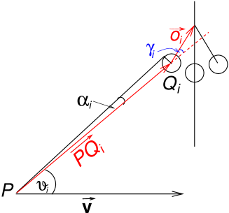
Figure 8.1: Definition of the variables used to calculate the total photo-electron number from the shower direction and the hits in the single OMs.

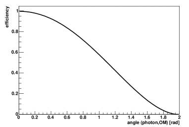
Figure 8.2: Parameterised angular efficiency $a_{i}$ of the ANTARES OMs, from [Cas99b].

One also has to take into account the attenuation $\Lambda_{att}$ of light in water:

$$\Lambda_{att}=e^{-|\overrightarrow{PQ_{i}}|/\tau}.$$

Here, $\tau$ is the attenuation length and has been set to 55 m, corresponding to the maximum absorption length at a wavelength of 475 nm (see Section 4.4.1). Scattering effects are not fully simulated by the light propagation software and are therefore not taken into account here; however, the effective scattering length at the ANTARES site is measured to be about 300 m, such that scattering would only slightly increase the photon attenuation.
Note that for these considerations, the Cherenkov light is assumed to be monochromatic. Because of this, also the quantum efficiency of the OMs is not taken into account as it is equal for all OMs and hence yields only an additional global normalisation factor. The goal of the calculations presented here is not to determine the true number of photons emitted from the shower, but to find a measure for the energy of the shower.

8.1.2 Angular Photon Distribution

It is assumed that the photons emitted by the shower are distributed uniformly in $\varphi$ and according to a distribution in $\vartheta$ obtained from Monte Carlo studies which has been shown in Figure 5.9. The distribution is shown again, together with the parameterisation presented in the following, in Figure 8.4. The distribution is characterised by a large, narrow peak at about 42^∘ and is slightly asymmetric, with a larger tail towards larger angles. It has therefore been parameterised by a Breit-Wigner-distribution with its maximum at the peak position and two Gaussians, one with its mean value approximately at the peak position and one with its mean at about 79^∘ to account for the tail; the parameterisation function $D(\vartheta,E_{sh})$ is given by:

$$D(\vartheta,E_{sh})=p\cdot\left(\frac{p_{0}}{\sqrt{2\pi}p_{1}}\cdot e^{-(\vartheta-p_{2})^{2}/(2p_{1}^{2})}+\frac{p_{3}}{\sqrt{2\pi}p_{4}}\cdot e^{-(\vartheta-p_{5})^{2}/(2p_{4}^{2})}+\frac{p_{6}}{2\pi}\frac{p_{7}}{(\vartheta-p_{8})^{2}+\frac{p_{7}^{2}}{4}}\right)$$ (8.1)

Here and in the following, $\vartheta$ is measured in degrees. The distribution implicitly depends on the shower energy $E_{sh}$, through the parameters $p_{0}$ to $p_{8}$. These parameters have been determined by fitting equation (8.1) to the photon distribution, at 11 different shower energy values between $\sim 560$ GeV and $\sim 56$ PeV, equally distributed in $\log_{10}E_{sh}$. The parameters have than been interpolated as functions of $\log_{10}E_{sh}$ as shown in Figure 8.3. Due to event-to-event fluctuations, it was not always possible to find a fit function for the whole energy range. The values for the parameters found at the lowest energies apparently do not fit to the overall shape of the parameter distributions and were left out in the fits. It will however be shown below that nevertheless, $D(\vartheta,E_{sh})$ describes the photon distribution at these energies well.
The parameterisations for the parameters are:

$$p_{0}= \,0.321 + \,0.0150 \cdot\log_{10}(E_{sh}/\textrm{GeV})$$

$$p_{1}= \,14.304 + \,0.336 \cdot\log_{10}(E_{sh}/\textrm{GeV})$$

$$p_{2}= \,40.791 + \,0.660 \cdot\log_{10}(E_{sh}/\textrm{GeV})$$

$$p_{3}= \,0.0779 - \,0.0137 \cdot\log_{10}(E_{sh}/\textrm{GeV}) +0.0055\cdot(\log_{10}(E_{sh}/\textrm{GeV}))^{2}$$

$$p_{4}= \,15.150 + \,2.843 \cdot\log_{10}(E_{sh}/\textrm{GeV})$$

$$p_{5}= \,78.694 - \,0.0367 \cdot\log_{10}(E_{sh}/\textrm{GeV})$$

$$p_{6}= \,0.688 - \,0.0506 \cdot\log_{10}(E_{sh}/\textrm{GeV})$$

$$p_{7}= \,6.181 - \,0.100 \cdot\log_{10}(E_{sh}/\textrm{GeV})$$

$$p_{8}= \,42.144 + \,0.0677 \cdot\log_{10}(E_{sh}/\textrm{GeV})$$

$D(\vartheta,E_{sh})$ is normalised to 1. The normalisation parameter $p$ is calculated analytically by solving the integral

$$\int_{0^{\circ}}^{180^{\circ}}\frac{D(\vartheta,E_{sh})}{p}\textrm{d}\vartheta\approx \int_{-\infty}^{\infty}\left(\frac{p_{0}}{\sqrt{2\pi}p_{1}}\cdot e^{-(\vartheta-p_{2})^{2}/(2p_{1}^{2})}+\frac{p_{3}}{\sqrt{2\pi}p_{4}}\cdot e^{-(\vartheta-p_{5})^{2}/(2p_{4}^{2})}\right)\textrm{d}\vartheta$$

$$+\int_{0^{\circ}}^{180^{\circ}}\left(\frac{p_{6}}{2\pi}\frac{p_{7}}{(\vartheta-p_{8})^{2}+\frac{p_{7}^{2}}{4}}\right)\textrm{d}\vartheta\qquad=\frac{1}{p}$$ (8.2)

which gives

$$p=(p_{0}+p_{3}+p_{6}/\pi\cdot(\arctan((360^{\circ}-2p_{8})/p_{7})-\arctan(-2p_{8}/p_{7})))^{-1}.$$ (8.3)

Here, the fact that the two Gaussian distributions in $D(\vartheta,E_{sh})$ have their maxima in the middle of the $\vartheta$-parameter space, at $\sim 43^{\circ}$ and $\sim 79^{\circ}$, and fall to very small values beyond $0^{\circ}$ and $180^{\circ}$, is used to allow for the approximate analytical calculation of the normalisation integral.

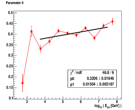
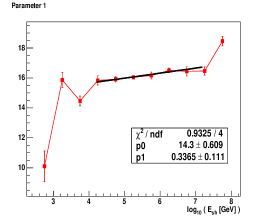
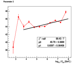
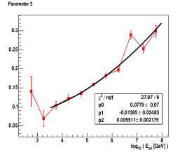
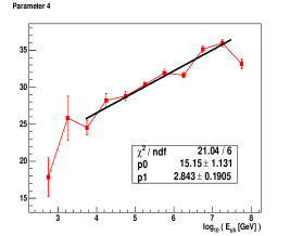
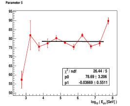
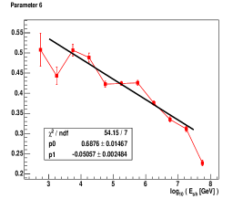
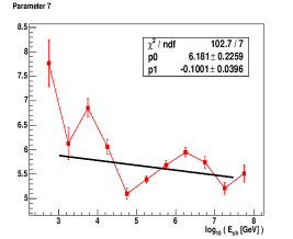
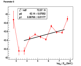
Figure 8.3: Energy-dependent values of the nine parameters in the function describing the $\vartheta$ distribution, $D(\vartheta,E_{sh})$, and fit curves to the values.

The main purpose of the parameterisation of the parameters was to find a fit which is in the ideal case a first degree polynomial, to keep equation (8.1) as simple as possible. The parameterisations presented here suffice to describe the distribution of $\vartheta$ for different energies, as can be seen from Figure 8.4, where the distribution of $\vartheta$ is displayed for the event sample A, together with the parameterisation $D(\vartheta,E_{sh})$, for energies between 300 GeV and 30 PeV (one decade per histogram). Here, $D(\vartheta,E_{sh})$ was calculated at the logarithmic centre of the respective energy bin. For angles $\leq 120^{\circ}$, the agreement between $D(\vartheta,E_{sh})$ and the photon distribution is very good. The slight deviations between $D(\vartheta,E_{sh})$ and the photon distribution at larger angles are insignificant for the calculation of the total photo-electron number.
It should be noted that for these studies the angle $\vartheta$ was calculated with respect to $\vec{r}_{\text{CG}}$, the OM-centre-of-gravity, as calculated in equation (7.8), not the interaction vertex. The reason for this is that this position is the outcome of the position reconstruction, as discussed in Section 7.1. Note also that during the fit, the momentary value of $E_{sh}$ is used for the determination of $D(\vartheta,E_{sh})$.

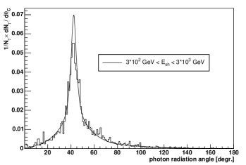
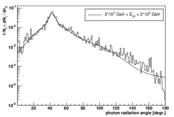
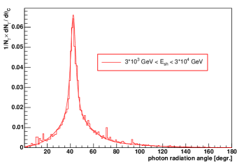
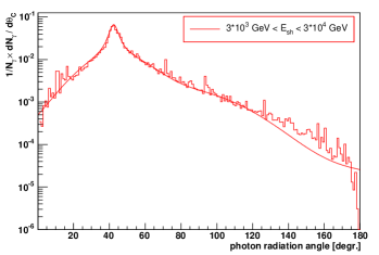
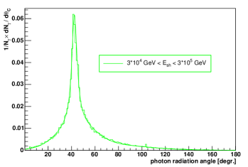
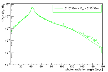
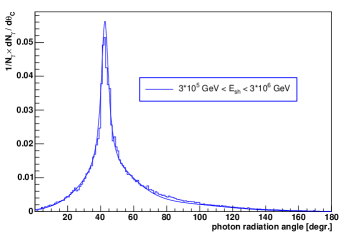
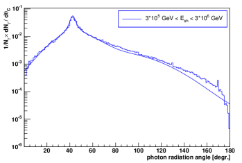
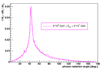
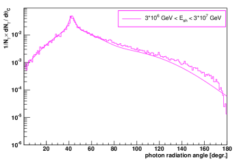
Figure 8.4: Angular distribution of the Cherenkov photons with respect to the shower axis for decades of energy between 300 GeV and 30 PeV, together with the parameterisation function for an energy in the logarithmic centre of the respective energy range (solid lines).

$D(\vartheta,E_{sh})$ has a similar shape also for energies larger or smaller than the ones studied here, so that also in the case of very large or very small energies, the photon distribution is still described approximately. However, it has to be ensured that none of the parameters $p_{0}$–$p_{8}$ becomes negative during the fit, which is achieved here by setting the lower limit of all parameters to $10^{-10}$.

8.1.3 Calculation of the Photo-Electron Number from the Hit Amplitudes

All the variables that are needed to calculate the photo-electron number $N_{i}$ in the event from the hit amplitude $n_{i}$ of hit $i$ in OM_i have now been collected. Starting point is the correction for the angular efficiency $a_{i}(\gamma_{i})$ of the OM:

$$n_{i}^{\prime}=\frac{n_{i}}{a_{i}(\gamma_{i})}.$$

Next, the photon attenuation is taken into account:

$$n_{i}^{\prime\prime}=\frac{n_{i}^{\prime}}{\Lambda_{att}}.$$

In the last step, the photons are distributed isotropically in $\varphi$ and according to $D(\vartheta,E_{sh})$ in $\vartheta$:

$$n_{i}^{\prime\prime\prime}=n_{i}^{\prime\prime}\cdot\frac{360^{\circ}\cdot\sin\vartheta_{i}}{2\alpha_{i}}\cdot\frac{1}{D(\vartheta_{i},E_{sh})\cdot 2\alpha_{i}}\equiv N_{i},$$

where $N_{i}$ is the total number of photo-electrons in the event according to hit $i$.
Altogether, one obtains:

$$N_{i}=\frac{n_{i}}{a_{i}(\gamma_{i})\cdot\Lambda_{att}}\cdot\frac{360^{\circ}\cdot\sin\vartheta_{i}}{2\alpha_{i}}\cdot\frac{1}{D(\vartheta_{i},E_{sh})2\alpha_{i}}.$$ (8.4)

$N_{i}$ is calculated independently for all hits $i$ in the event. After this, the median of all $N_{i}$ is calculated; this value is then used as a starting value for the number of photo-electrons produced by this shower, which is directly proportional to the shower energy. Figure 8.5 shows exemplarily the distribution of the photo-electron numbers calculated once for every hit in an event, for a selection of five events from event sample A with different energies. Though for most events there is a clear trend towards one favourable value for the photo-electron number, the values of the photo-electron numbers calculated from each hit can be very widely spread, mainly due to the angular acceptance $a_{i}(\gamma_{i})$ which decreases to very small values for incident angles larger than $\sim 115^{\circ}$ (see Figure 8.2). Therefore, to obtain one single and reliable value for the photo-electron number in the event, the median was chosen; it is more stable against wide spreads of the values than the arithmetic mean. The MC shower energy plotted versus the median of the photo-electron numbers calculated in the described way is shown in Figure 8.6 for event sample A.

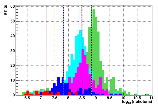
Figure 8.5: Photo-electron number in 5 events as calculated from the hit amplitudes in every hit OM; the values for each event are marked by different colours. The respective values of the medians are also shown as dashed lines.

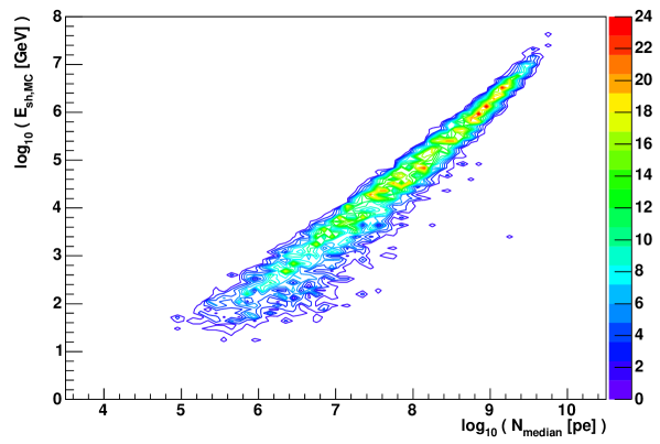
Figure 8.6: Monte Carlo shower energy over the median of the photo-electron numbers $N_{i}$, calculated from the hit amplitude $n_{i}$ in all OMs, as described in the text.

8.1.4 Comparison of the Measured and the Calculated Hit Amplitudes

To calculate the expected amplitude $n_{i,c}$ in OM_i from the total number of photo-electrons $N$, position, direction and energy of the shower are needed. The position is calculated following the algorithm from Section 7.1, and for the shower direction, a starting value is assumed from a scan of the parameter space (see Section 8.2.1). The shower energy can be calculated from the total number of photo-electrons $N$ (see Section 8.2.2). By inverting equation (8.4), $n_{i,c}$ is calculated as

$$n_{i,c}=N\cdot a_{i}(\gamma_{i})\cdot\Lambda_{att}\cdot\frac{2\alpha_{i}}{360^{\circ}\cdot\sin\vartheta_{i}}\cdot D(\vartheta_{i},E_{sh})\cdot 2\alpha_{i}.$$ (8.5)

$n_{i,c}$ can then be compared with $n_{i,meas}$, the actually measured amplitude in OM_i. The lower limit of $n_{i,meas}$ is the SPE threshold (see Section 4.3.1); measured amplitudes below the threshold are considered as noise. For this study, an SPE threshold of 0.3 pe was used. The measurement process in the photomultiplier smears the number of photo-electrons, so that the probability to measure a signal $n_{i,meas}$ when $j$ photo-electrons were generated in the photomultiplier is

$$P_{g}(n_{i,meas},j)=\frac{1}{\sigma_{j}\cdot\sqrt{2\pi}}\cdot e^{-(n_{i,meas}-j)^{2}/(2\sigma_{j}^{2})},\qquad j>0.$$ (8.6)

The width $\sigma_{j}$ depends on the number of photo-electrons $j$. It has been calculated for ${1\leq j\leq 210}$ as proposed by [Kop05]: For each $j$, a measurement is simulated $5\cdot 10^{8}$ times using the ANTARES photomultiplier simulation [Cas99b]. A Gaussian fit is the applied to the resulting distribution of $n_{i,meas}$; the width of the fit is the desired $\sigma_{j}$. The values of $\sigma_{j}$ calculated that way are as shown in Figure 8.7.

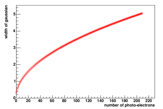
Figure 8.7: Width $\sigma$ of the Gaussian distribution (8.6) for signals between 1 and 210 photo-electrons.

The probability $P_{g}(n_{i,meas},0)$ to measure an amplitude $n_{i,meas}$ if no photo-electrons at all been produced in the OM, i.e. to measure electronics noise, must be taken into account as well. For the analysis of real data, the individual calibration data for each OM would have to be used to determine the noise pedestal (see Figure 4.10). The minimum threshold would have to be adjusted for each event, as is is set according to the current optical noise. For this MC based study, the noise term is estimated as an exponentially decreasing function, with ${P_{g}(n_{i,meas},1)\geq P_{g}(n_{i,meas},0)}$ above the minimum threshold $n_{i,meas}=0.3$:

$$P_{g}(n_{i,meas},0)=0.99\cdot e^{-10\cdot n_{i,meas}}.$$ (8.7)

The factor 0.99 is used to ensure $P_{g}(n_{i,meas},0)<1$.
The relation between the expected amplitude $n_{i,c}$ and the actual photo-electron number $j$ can be described by a Poissonian distribution:

$$P_{p}(n_{i,c},j)=\frac{n_{i,c}^{j}}{j!}\cdot\textrm{e}^{-n_{i,c}}.$$ (8.8)

If the expected amplitude is $n_{i,c}$, the probability $l_{i,j}$, that $j$ photo-electrons have been produced which generate a measured amplitude $n_{i,meas}$, is the product of the two probabilities $P_{p}(n_{i,c},j)$ and $P_{g}(n_{i,meas},j)$:

$$l_{i,j}=P_{p}(n_{i,c},j)\cdot P_{g}(n_{i,meas},j).$$ (8.9)

Summing over all $j$ gives the probability to measure $n_{i,meas}$ if $n_{i,c}$ is expected:

$$L_{i}(n_{i,meas},n_{i,c})=\sum^{j_{max}}_{j=j_{min}}l_{i,j}=\sum^{210}_{j=0}P_{p}(n_{i,c},j)\cdot P_{g}(n_{i,meas},j).$$ (8.10)

The lower limit of the summation represents the case of no photo-electrons being produced in OM_i, while the upper limit of 210 is 10 pe above the saturation of the photomultiplier electronics of 200 pe. In principle, both in simulation and in measurement, a signal of 200 pe can also be caused by more than 200 photo-electrons, such that the upper limit of $j$ could be chosen arbitrarily large. However, both $P_{g}(n_{i,meas},j)$ and $P_{p}(n_{i,c},j)$ decrease rapidly for large $j$, and it is therefore possible to set the upper summation limit slightly above the saturation limit, at 210.
$L_{i}$ is the function which determines the likelihood of the combination $n_{i,meas}$ and $n_{i,c}$ in OM_i. Therefore, the overall probability $\mathcal{P}$ for a hit constellation in the whole detector is given by multiplying the probabilities of the single OMs:

$$\begin{split}\mathcal{P}&=\prod_{i=1}^{900}L_{i}=\prod_{i=1}^{900}\sum^{210}_{j=0}P_{p}(n_{i,c},j)\cdot P_{g}(n_{i,meas},j)\\ &=\prod_{i=1}^{900}\sum^{210}_{j=0}\frac{n_{i,c}^{j}}{j!}\cdot\textrm{e}^{-n_{i,c}}\cdot P_{g}(n_{i,meas},j)\\ &=\prod_{i=1}^{900}\sum^{210}_{j=0}\left(\frac{(N_{i}\cdot a_{i}(\gamma_{i})\cdot\Lambda_{att}\cdot\frac{2\alpha_{i}}{360^{\circ}\cdot\sin\vartheta_{i}}\cdot D(\vartheta_{i},E_{sh})\cdot 2\alpha_{i})^{j}}{j!}\right.\\ &\hskip 45.52458pt\left.\cdot\,\textrm{exp}\{-(N_{i}\cdot a_{i}(\gamma_{i})\cdot\Lambda_{att}\cdot\frac{2\alpha_{i}}{360^{\circ}\cdot\sin\vartheta_{i}}\cdot D(\vartheta_{i},E_{sh})\cdot 2\alpha_{i})\}\cdot P_{g}(n_{i,meas},j)\right).\end{split}$$ (8.11)

8.2 The Maximum Likelihood Fit

The shower direction and energy are determined by maximising the likelihood in equation (8.11). In this process, the log likelihood $\ln\mathcal{P}$ is considered instead of $\mathcal{P}$. By multiplying the expression with $-1$, the maximisation problem is replaced by a minimisation. The final expression to be minimised becomes therefore

$$\mathcal{L}=-\ln\mathcal{P}=\sum_{i=1}^{900}(-\ln(L_{i})).$$ (8.12)

To minimise $\mathcal{L}$, the fitting software MINUIT [Jam98] which was developed at CERN is used. The technical details of the minimisation are explained in appendix B, where also a chart of all steps of the reconstruction can be found.

8.2.1 Starting Values for the Fit

To start the fit, suitable values for the three parameters $\theta,\phi$ and $E_{sh}$ are needed. They are determined by scanning the whole parameter space. The scan is done by calculating the value of the likelihood function for a selectable number of data points. For the results shown in the following, 15 points were used for $\theta$ and $\phi$ each, and 5 for the photo-electron number, so that the likelihood was calculated at $15\times 15\times 5$ points. The 15 points of the directional variables were equally distributed, between $-\pi$ and $\pi$ in $\phi$ and between $-1$ and $1$ in $\cos\theta$. The 5 points for the photo-electron number were equally distributed between $\log_{10}(N_{m})-2$ and $\log_{10}(N_{m})+2$, where $N_{m}$ is the median of the total photo-electron numbers calculated for all hits in the event, as described in Section 8.1.3. The reconstructed position of the shower, calculated as described in Section 7.1, and the shower direction, calculated under the assumption that all photons are emitted from the shower under the same angle $\vartheta_{C}$, as described in Section 7.2.1, were used as input variables for the calculation of $N_{m}$.
The parameter values for which the likelihood is smallest are then used as starting values for the actual fit. These starting values are often already quite close to the MC values, as can be seen from Figures 8.8 and 8.9, where the values of $\theta,\phi$ and the photo-electron number from the scan are plotted versus the respective MC values. While the bins for the likelihood calculation are visible in $\theta$ and $\phi$, for the photo-electron number this is not the case, because $N_{m}$ is different in each event.

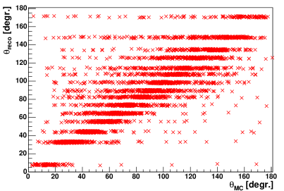
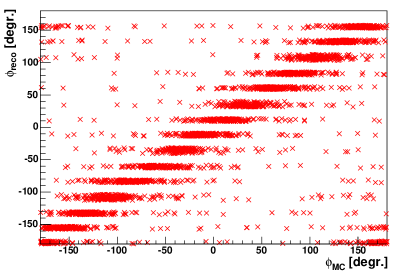
Figure 8.8: Fit variables $\theta$ and $\phi$ as determined by a scan of the likelihood parameter space drawn over their respective MC values. One can see that the algorithm is sufficient in most cases to find a parameter value close to the MC value.

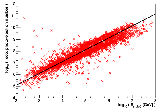
Figure 8.9: The fit variable “photo-electron number” as determined by a scan of the likelihood parameter space, vs. the MC shower energy. The linear function (8.13) which is used to calculate the shower energy from the photo-electron number is also shown.

8.2.2 Calculation of Neutrino Energy from the Photo-Electron Number

A formula to calculate the energy of the hadronic shower from the reconstructed photo-electron number was determined from successfully reconstructed events, by comparing the reconstructed photo-electron number to the MC shower energy. Here, a sample of 140000 NC events between 10 GeV and 10 PeV was used (event sample B, see Appendix A.5.1). The events were reconstructed by minimising equation (8.12); Figure 8.10 shows the distribution of those events for which the direction was reconstructed with an error smaller than $10^{\circ}$, and a parameterisation of the correlation between photo-electron number and MC energy,

$$\log_{10}(E_{sh}/\textrm{GeV})=-3.03+0.99\cdot\log_{10}N.$$ (8.13)

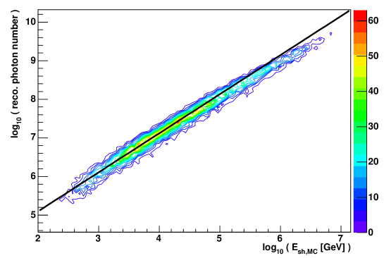
Figure 8.10: MC shower energy over reconstructed photo-electron number, for events with an angular error $<10^{\circ}$, together with the fit from equation (8.13).

Function (8.13) is valid within the energy range of $10^{3}$ GeV$\leq E_{sh}\leq 10^{5.2}$ GeV. For lower and higher shower energies, the distribution is bent towards smaller photo-electron numbers.
The shower energy can thus be calculated from the photo-electron number. However, to retrieve the neutrino energy is not straight-forward, as for NC events a fraction of $(1-y)$ of the primary neutrino energy (where $y$ is the Bjorken variable, see Section 3.1.1) goes into the secondary neutrino. Therefore, the shower energy as calculated from the reconstructed photo-electron number only yields a lower limit on the primary neutrino energy. On the other hand, in the CC reaction of $\nu_{e}$, all neutrino energy goes into showers, and the signature of this event type will not be distinguishable from that of NC events, so that in the end the energy calculated using equation (8.13) is to be regarded as the neutrino energy. The comparison with the MC neutrino energy should then, for a combined sample of shower-type events, lead to a narrow peak at ${E_{sh}=E_{\nu}}$ for the $\nu_{e}$ CC events, with a long tail towards the region of a reconstructed energy that is smaller than the MC neutrino energy, as shown in Figure 8.11. For this plot, events with an angular error smaller than $10^{\circ}$ were selected from event sample B (NC events) and from the $\nu_{e}$ CC event sample (see Appendix A.5.2).

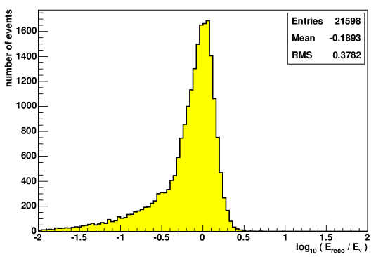
Figure 8.11: Error in reconstructed neutrino energy for a mixed sample of shower-type events reconstructed with an angular error smaller than $10^{\circ}$.

8.2.3 Examination of the Likelihood Parameter Space

From the description of the likelihood function given in the above sections it is in principle possible to reconstruct any kind of shower-type event producing hits in the detector. In reality, however, it is important for the success of the reconstruction where, with respect to the instrumented volume, an interaction took place, and whether this position is well reconstructed or not. In this section, several different event topologies are presented. The list of topologies is by no means exhaustive, but it gives an overview of the possible problems that might be encountered in the event reconstruction.

The Ideal Event

The ideal shower-type event is that of a neutrino which interacts inside the detector, so that the whole shower is right in the middle of the instrumented volume. In Figures 8.12, 8.13 and 8.14, the shape of the likelihood function for three well-reconstructible events is shown. The log likelihood is calculated for the variation of one of the three fit parameters, keeping the other two parameters constant at their true values or at their final values from the fit. The true MC value and the reconstructed value are also shown. The events shown in Figures 8.12 and 8.13 had similar shower directions, but different shower energies of $E_{sh}=3.7$ TeV and $E_{sh}=19$ TeV, respectively. The event shown in Figure 8.14 had a shower energy of $E_{sh}=269$ TeV. For the variation of the photo-electron number, the shape of the likelihood is similar in all three events, and very smooth. For the variation of $\theta$ and $\phi$, the likelihood shows larger fluctuations; a clear global minimum is visible in all cases, but a number of local minima is present as well. The neutrino shown in Figure 8.14 had a large zenith angle, i.e. it came from above; it interacted not far away from the upper edge of the detector. Even though the resolution for the reconstruction of downgoing events is generally worse than for upgoing events (due to the orientation of the photomultipliers, see also Section 9.5), this example shows that a good reconstruction is also possible for this event type (total angular error in this case: $1.65^{\circ}$).
Snapshots of the three events in the ANTARES event display [Hei05] are shown in Figure 8.15. For better visibility, only hits passing the filter conditions (see Section 6.4) are displayed.

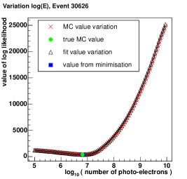
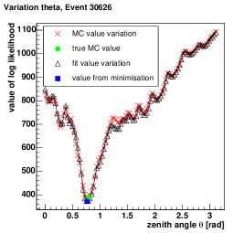
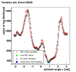
Figure 8.12: Values of the likelihood function for the variation of the photo-electron number (left), the zenith angle $\theta$ (middle) and the azimuth angle $\phi$ (right), for a well-reconstructible event. The plots show the log likelihood calculated for the variation of one of the three fit parameters, keeping the other two parameters constant at their true values (red crosses) or their final values from the fit (black triangles). The true MC value (green circle) and the reconstructed value (blue square) are also shown.

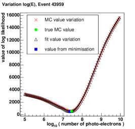
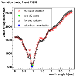
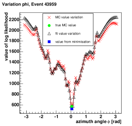
Figure 8.13: Values of the likelihood function for the variation of the photo-electron number (left), the zenith angle $\theta$ (middle) and the azimuth angle $\phi$ (right), for a well-reconstructible event. See Figure 8.12 for details.

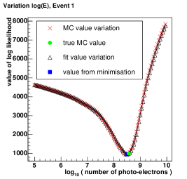
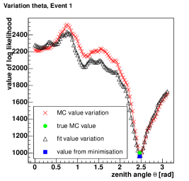
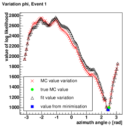
Figure 8.14: Values of the likelihood function for the variation of the photo-electron number (left), the zenith angle $\theta$ (middle) and the azimuth angle $\phi$ (right), for a well-reconstructible event induced by a downgoing neutrino. See Figure 8.12 for details.

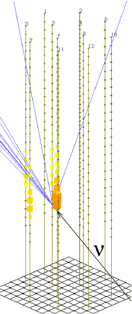
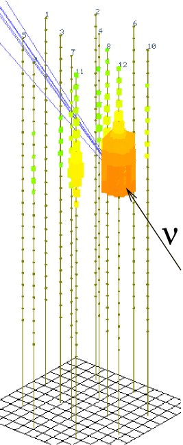
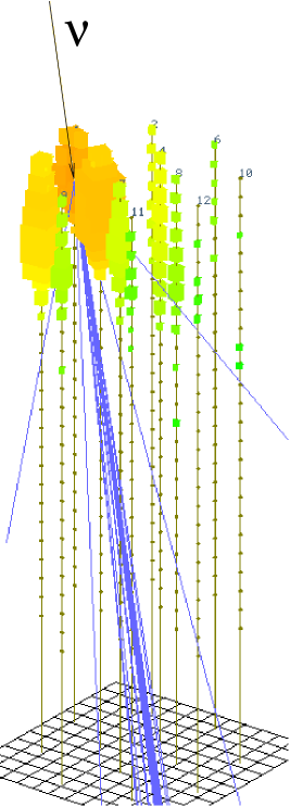
Figure 8.15: Events from Figures 8.12, 8.13 and 8.14 as seen in the ANTARES event display. The detector strings are shown as numbered lines, with dots marking the different storeys. The incident neutrino is shown in black, the blue lines mark the particle tracks of the shower (not to scale), and the squares show the photo-electron signals, integrated over 25 ns. The size of the squares is proportional to the hit amplitude, and their colour coding is according to the arrival time of the first photon in the photomultiplier, from red over yellow to green.

Impacts of Shifts in the Shower Position

The success of the direction and energy depends on the accuracy of the reconstructed position of the shower. If the position is wrong by several ten metres (e.g. inside the instrumented volume instead of outside), the shape of the likelihood function can change significantly, and a correct reconstruction of direction and energy is not possible. Even if the position is only wrong by a few metres, the reconstruction can end up with totally different results. As examples, the well reconstructed event shown above in Figure 8.14 is displayed again in Figure 8.16, for varied positions, as explained below. The event takes place inside the instrumented volume (i.e. it is contained). Figure 8.17, on the other hand, displays an event whose interaction vertex is outside the instrumented volume, a so called non-contained event. The latter yields a large angular error after reconstruction. For both events, the likelihood function was calculated varying one of the three parameters, as above, and keeping the others constant at their MC values. The true value of the respective parameter is again marked by a green circle. The other two distributions show the values of the likelihood, again varying one parameter and keeping the others at their MC values, but with a position that is shifted 6 m along the MC shower axis, once forward in shower direction, and once backward, against the shower direction. For the contained event, the shape of the likelihood varies slightly with these shifts, but the position of the global minimum remains relatively stable. For the non-contained event, however, there is a second minimum in the likelihood for the variation of $\theta$, which becomes deeper than the one containing the MC value, if the position is shifted in forward direction. Though the shower reconstruction algorithm describes the event correctly, which can be seen from the fact that the MC values are located in the global minimum of the parameter space, the ambiguities are large enough to create a second, deep local minimum which can become global for slight shifts in the position. It should also be noted that the difference between the two minima in $\theta$ is approximately twice the Cherenkov angle of $42^{\circ}$.

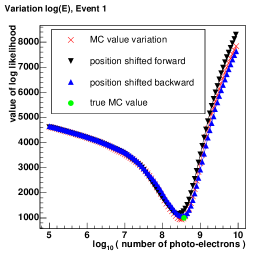
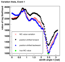
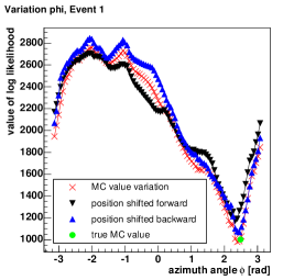
Figure 8.16: Values of the likelihood function using the true position and two positions shifted along the shower axis, varying the photo-electron number (left), the zenith angle $\theta$ (middle) and the azimuth angle $\phi$ (right), for a well-reconstructed event.

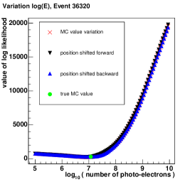
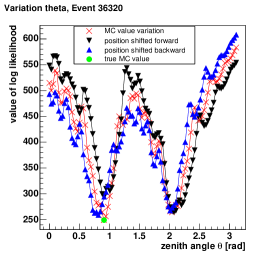
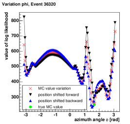
Figure 8.17: Values of the likelihood function using the true position and two positions shifted along the shower axis, varying the photo-electron number (left), the zenith angle $\theta$ (middle) and the azimuth angle $\phi$ (right), for a non-contained event.

Non-contained Events

Because of the directional characteristics of showers, non-contained events, i.e. events whose interaction vertex lies outside the instrumented volume, are very difficult to reconstruct, as the fact that only one side of the detector measures incident photons induces a bias in the signal. What adds to this is that for these events the position reconstruction as described in Section 7.1 is more likely to fail. In such a case it is almost impossible to get good results from the reconstruction of direction and energy, as the fit then minimises the likelihood using wrong assumptions. As an example for this, the shape of the likelihood function for a badly reconstructed event is shown in Figure 8.18. For this event, the interaction vertex lies outside the instrumented volume at the point (-82, 120, -160) in the ANTARES coordinate system, where (0, 0, 0) lies right in the centre of the detector, and the detector edge lies approximately at $(\pm 100,\pm 100,\pm 175)$. The position was reconstructed at (-56, 72, -136), inside the instrumented volume, with a large positional error. For the reconstructed position, the measured hit amplitudes in the individual OMs do not match the true direction of the shower. The azimuth angle $\phi$ is flipped to the opposite direction. As the $z$ coordinate is reconstructed 24 m too large, the shower seems to be downgoing (i.e. $\theta>\pi/2$); consequently, the zenith angle $\theta$ is reconstructed too large. Because of the worse acceptance of the OMs for downgoing photons, also the shower energy is overestimated, as can be seen from the left plot of Figure 8.18.

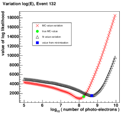
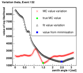
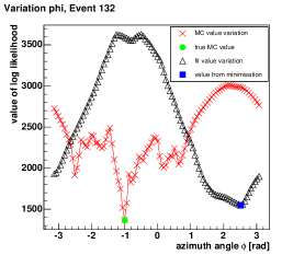
Figure 8.18: Values of the likelihood function for the variation of the photo-electron number (left), the zenith angle $\theta$ (middle) and the azimuth angle $\phi$ (right), for a non-contained, poorly reconstructed event.

Events Close to the Detector Edge

Neutrinos which produce showers at the edge of the detector, such that the largest part of the signal is measured by a few strings at one side of the detector, are not as problematic as non-contained events. However, also these events cannot always be reconstructed well. The reason for this is that the likelihood description sometimes lacks the necessary information for a successful reconstruction, because only one side of the shower or even less is visible for the detector. However, the fact that the shower is happening close to the detector edge does not necessarily mean that this event will be badly reconstructed. In fact, quite a number of such events are still reconstructed well, so that it is difficult to decide from the reconstructed position or other criteria if the result of a reconstruction is unreliable and the event should be discarded.
An example for the variation of the likelihood function of a well reconstructed edge event are shown in Figure 8.20. The event display for this event is shown in Figure 8.20. As before, again the values of the likelihood function is shown in Figure 8.20, varying one of the parameters, and keeping the others either at their MC or at their reconstructed values. One can see from the upmost plot of Figure 8.20 that the energy of this event is relatively large; this is the reason for the large detector signal, despite the fact that the neutrino is pointing to the outside the instrumented volume. The shapes of the likelihood function using the MC or the reconstructed values are very similar. The distributions are characteristical for an edge event: They display only one minimum, as there is only one possible orientation of the shower with respect to the measured hit pattern; and the minimum is relatively broad for $\theta$ and $\phi$, because the information obtained from the measurement is not as precise as would be the case for an interaction in the middle of the detector.

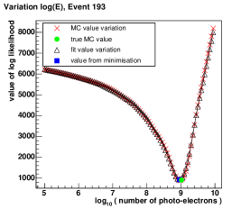
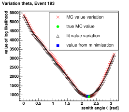
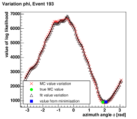
Figure 8.19: Values of the likelihood function for the variation of the photo-electron number (top), the zenith angle $\theta$ (middle) and the azimuth angle $\phi$ (bottom), for an edge event.

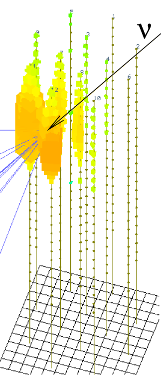
Figure 8.20: Edge event from Figure 8.20 as seen in the ANTARES event display. Only the hits passing the filter conditions are shown.

8.2.4 Numerical Stability Check

Steps or jumps in the likelihood function can prevent the fit from converging, because the gradient cannot be calculated at these likelihood values and therefore the fit does not “know”  in which direction to continue. The steps can be caused e.g. if fit parameters have a limited validity range. The likelihood function therefore has to be carefully checked for instabilities. Additionally, the numerical precision of the calculation is an intrinsic feature which can cause problems if the precision of the fit parameters becomes equal or higher, which would let the fit run into numerical noise, causing uncontrolled, random steps and preventing any further convergence. It is therefore important to ensure that all values in the function are calculated with double precision. This is usually not guaranteed just by setting all the user’s variables to double precision, as the single precision could also be used in an external function over which the user does not have control.
A safe way to ensure that neither steps caused by limits of the likelihood parameter space nor jumps caused by numerical noise lead to problems in the fit is to examine the likelihood parameter space by keeping all but one of the fit parameters constant at the minimum of the likelihood function and varying the remaining parameter in very small intervals around the minimum.
Examples for this are shown in figures 8.21 and 8.22 for the variation of two variables of the same event. In these figures, the size of the interval inside which the likelihood was calculated is decreased by a decade for each subsequent plot. In Figure 8.21, the likelihood was calculated at the fixed fit values for $\phi$ and the photo-electron number, and $\theta$ was varied around the fit value in the steps given in the header of the respective graph. Plotted in the graphs is the difference between the varied value of $\theta$ and the value reached as the final result of the fit. Down to a precision of $10^{-6}$, which was the chosen precision of the minimisation for this example, the fit value, marked by the blue square, always lies at the lowest point of the graph, as expected. Numerical noise only starts at a precision of $10^{-11}$, and besides this noise there are no other steps visible in the graphs. The same is true for Figure 8.22, where $\phi$ was varied instead of $\theta$.
The calculations shown in this subsection have been done for a several dozen events with different characteristics, i.e. different shower directions and energies. It was concluded that stability problems do not influence the fit.

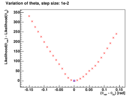
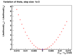
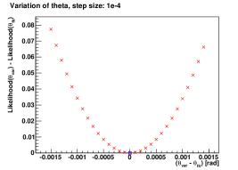
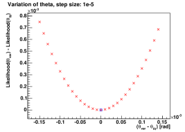
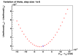
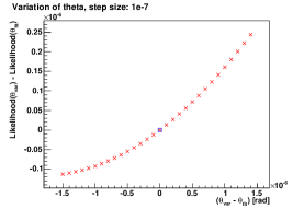
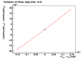
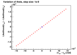
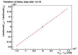
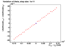
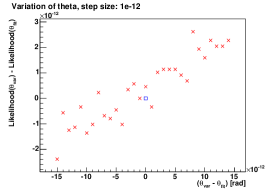
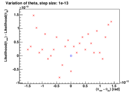
Figure 8.21: Values of the likelihood function for variations of $\theta$ around the fit value.

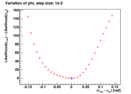
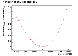
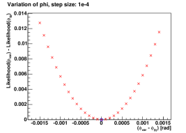
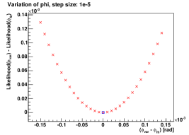
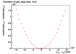
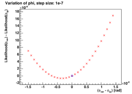
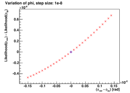
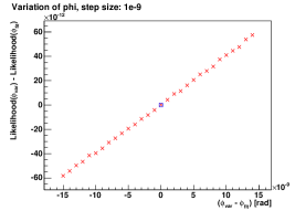
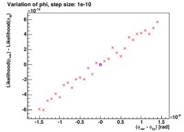
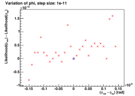
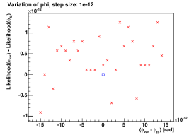
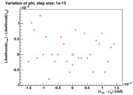
Figure 8.22: Values of the likelihood function for variations of $\phi$ around the fit value.

Conclusion

In this chapter, a method has been described which allows the combined reconstruction of the direction and energy of a shower, using the shower position as calculated in Section 7.1 together with directional and energy estimates from a scan of the likelihood parameter space as starting values. Studies of the likelihood parameter space show that the introduced pattern matching algorithm describes the shower very well (see also Chapter 10, where results both for NC events and for $\nu_{e}$ CC events are presented). Not all events can be reconstructed equally successfully; unfortunate event topologies will sometimes prevent a good result. Quality cuts to distinguish poorly reconstructed events from well reconstructed ones will be discussed in the following chapter.

Chapter 9 Quality Cuts for the Event Selection

Clearly, not all shower-type events are reconstructible with the same precision, and some events are not usable for physics analysis. If there is a problem with the convergence of the minimisation, the fit program itself will notice this, and the reconstruction will be aborted. However, sometimes events cannot be reconstructed well because their shape does not agree with the assumed model. This is the case e.g. if an event has touched only the edge of the detector, producing enough hits to pass the filter conditions but not enough information in the hits to allow for a good reconstruction, or if the position of the shower has been miscalculated and therefore the likelihood function does not have a minimum close to the true values of the parameters (cf. Section 8.2.3).
Quality cuts are used to separate the poorly reconstructed events from the well reconstructed ones, and to separate off events which are no shower events at all. The latter refers especially to atmospheric muon events which might be misinterpreted as shower events if they consist of several muons in a bundle, or if the muon undergoes a catastrophic bremsstrahlung loss and thereby produces an electromagnetic cascade (see Section 6.1).
In Section 9.1, the suppression of this atmospheric muon background is discussed. Sections 9.2 to 9.6 discuss quality cuts that are intended to allow for the separation of well reconstructed events from poorly reconstructed ones. Note that only the cuts introduced in Sections 9.1.1, 9.3 and 9.4 are used as final quality cuts on the events, as they showed the best efficiencies and purities. Efficiencies and purities of all the cuts introduced here are summarised in Section 9.7
Within this chapter, a separation of events according to the angular misreconstruction of the shower direction with respect to the MC shower axis will be made. Events with a deviation $\Delta\alpha<10^{\circ}$ will be considered as good events, those with ${10^{\circ}\leq\Delta\alpha<30^{\circ}}$ as moderate events and those with $\Delta\alpha\geq 30^{\circ}$ as bad events. As the quality of the reconstruction also depends on the shower energy, the events will be grouped in three different energy bins: $E_{sh}<10$ TeV, 10 TeV $\leq E_{sh}<1$ PeV and $E_{sh}\geq 1$ PeV, where $E_{sh}$ is the MC shower energy. The shower energy and the neutrino direction are strongly correlated; therefore, a badly reconstructed direction will in many cases go along with a badly reconstructed energy.
The effects of the cuts will be shown for two different data samples, namely, a sample of 140000 NC events (event sample B, see Appendix A.5.1), and a sample of $\nu_{e}$ CC events of about the same size (see Appendix A.5.2). About 18000 events (13.0%) of the NC sample, and 31000 events (22.5%) of the $\nu_{e}$ CC sample remain in the sample after the optical background filter and the reconstruction. The number of events passing filter and reconstruction highly depends on the neutrino energy (see Figure A.2) and the generation volume, which exceeded the instrumented volume by one absorption length ($\sim 55$ m). The reason for the higher efficiency for the $\nu_{e}$ CC events is that for these events the entire energy of the primary neutrino is transfered into the electromagnetic and hadronic shower, while for NC events the average fraction of the primary energy which is transfered to the hadronic shower is only between $\sim 32\%$ and $\sim 46\%$, depending on the neutrino energy (see Figure 3.3 in Section 3.1.1).
The numbers of events for the different energy bins and reconstruction qualities, before all cuts, are shown in Table 9.1. See Figure A.2 and Tables A.1 and A.2 (Appendix A.5) for more details.

NC events	good	moderate	bad	total
$E_{sh}<10$ TeV	3318	2527	3568	9413
10 TeV $\leq E_{sh}<1$ PeV	4082	2113	1943	8138
$E_{sh}\geq 1$ PeV	382	152	144	678
total	7782	4792	5655	18229

$\nu_{e}$ CC events	good	moderate	bad	total
$E_{sh}<10$ TeV	6201	4148	6317	16666
10 TeV $\leq E_{sh}<1$ PeV	6135	3103	2759	11997
$E_{sh}\geq 1$ PeV	1480	523	495	2498
total	13816	7774	9571	31161

Table 9.1: Number of well, moderately and badly reconstructed events in three energy bins, before all cuts (see text for definitions).

9.1 Suppression of Atmospheric Muons

For the investigation of atmospheric muons, a CORSIKA [Hec98] simulation with protons as primary cosmic rays was used. Protons are the dominating contributors to the cosmic radiation, at least up to the “knee”  at about 4 PeV [Hoe05]. Muons produced by the interaction of the protons in the atmosphere can produce a signal in the ANTARES detector. The event sample used for this study was taken from the ANTARES MC data repository (see Appendix A.5.3 for more details on the data sample).
Those events of the muon sample that arrived at the instrumented volume and produced hits in the detector were processed through the shower reconstruction. For a large number of these atmospheric muon events, the fit does not converge; those events are thus not reconstructed.

9.1.1 Expected and Measured Amplitudes: Quality Cut

For the rejection of the atmospheric muons remaining after the reconstruction, it is useful to consider the correlation between the amplitudes expected in each OM according to the result of the direction and energy reconstruction, and the measured amplitudes. Even though those atmospheric muons which survive the reconstruction have an event signature similar to that of shower events, there are significant differences in the hit pattern, as muons produce hits with small amplitudes along the muon trajectory, whereas showers produce relatively localised, large hits.
As a measure for the difference between the amplitude $n_{i,c}$ expected for the reconstructed direction and energy, and the measured amplitude $n_{i,meas}$ in each OM, a variable $\xi$ is defined:

$$\xi=\frac{1}{N}\sum_{i=1}^{N}\frac{(n_{i,c}-n_{i,meas})^{2}}{{n_{i,c}}^{2}}.$$ (9.1)

Here, $N$ is the number of OMs for which $n_{i,c}$ or $n_{i,meas}$ are above the minimum threshold of 0.3 pe. The variable $\xi$ is expected to be distributed very differently for muon events than for shower events, because of the large number of small amplitude hits that a muon produces in OMs where no signal is expected by the shower reconstruction strategy.
Figure 9.1 shows the distribution of $\xi$ for shower events on the left hand side, and for muons on the right hand side. The distributions for shower events have their maximum at ${\log_{10}\xi\approx 0}$, i.e. $\xi\approx 1$, for all reconstruction qualities. However, the distribution of the poorly reconstructed events (green histogram in Figure 9.1) extends to larger values of $\xi$, because the agreement between the calculated and the measured amplitudes is worse for these events, compared to the moderately and well reconstructed ones. The plot shown here was generated using NC events; for $\nu_{e}$ CC events, the distribution is very similar, as can also be seen from the event numbers after a cut on $\log_{10}\xi<0.2$ (see Table 9.2). The cut applied at ${\log_{10}\xi<0.2}$ keeps $66\%$ of the well and moderately reconstructed shower-type events in the data sample, while $80\%$ of the poorly reconstructed shower events are suppressed.
The atmospheric muon events, on the right hand side of Figure 9.1, are distributed towards much larger values of $\xi$, with a peak around ${\log_{10}\xi\approx 4}$. Most of the muon events are rejected by the cut at ${\log_{10}\xi<0.2}$.
Figure 9.2 displays the distribution of $\xi$ versus the reconstructed shower energy. Due to the increasing number of large hits for higher energies, the $\xi$ distribution of the shower events decreases with increasing energy. For the atmospheric muons, the opposite is the case: For the highest energies, almost no events remain in the sample.
Table 9.3 lists the numbers of muon events remaining in different angular and energy bins after the reconstruction and the cut. A comparison between the remaining atmospheric muon event rate and that of the neutrino signal is given in Section 10.4.

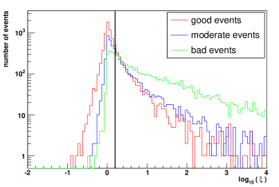
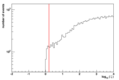
Figure 9.1: Variable $\xi$ as defined in equation (9.1), for the NC event sample B (left), and for the atmospheric muons (right). The position of the cut is also indicated.

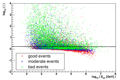
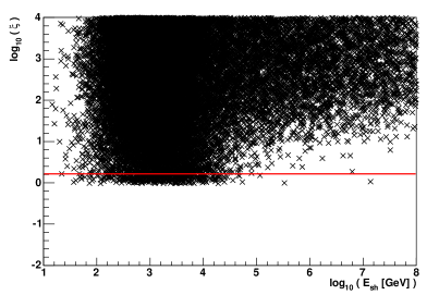
Figure 9.2: $\xi$ over the reconstructed shower energy, for the NC event sample B (left), and for the atmospheric muons (right). The position of the cut is also indicated.

NC events	good	moderate	bad	total
$E_{sh}<10$ TeV	2135 (64.3%)	1071 (42.4%)	540 (15.1%)	3746 (39.8%)
10 TeV $\leq E_{sh}<1$ PeV	3356 (82.2%)	1424 (67.4%)	657 (33.8%)	5437 (66.8%)
$E_{sh}\geq 1$ PeV	347 (90.8%)	120 (78.9%)	61 (42.4%)	528 (77.9%)
total	5838 (75.0%)	2615 (54.6%)	1258 (22.2%)	9711 (53.3%)

$\nu_{e}$ CC events	good	moderate	bad	total
$E_{sh}<10$ TeV	3758 (60.6%)	1576 (38.0%)	772 (12.2%)	6106 (36.6%)
10 TeV $\leq E_{sh}<1$ PeV	4914 (80.1%)	2053 (66.2%)	863 (31.3%)	7830 (65.3%)
$E_{sh}\geq 1$ PeV	1385 (93.6%)	434 (83.0%)	224 (45.3%)	2043 (81.8%)
total	10057 (72.8%)	4063 (52.3%)	1859 (19.4%)	15979 (51.3%)

Table 9.2: Number of good, moderate and bad shower events in the three energy bins, after the cut on $\log_{10}\xi<0.2$; the percentages were calculated with respect to the number of events after the reconstruction, as displayed in Table 9.1.

angle	$0^{\circ}-60^{\circ}$
primary energy [TeV/nucleon]	1-10	10-100	100-105
generated events	$10^{8}$	$10^{7}$	$10^{7}$
events producing hits	917045	419280	2383537
events after reconstruction	966	2002	76803
events after $\xi$ cut	11	32	472
event rate after cut	7.51 h-1	7.73 h-1	2.187 h-1

angle	$60^{\circ}-85^{\circ}$
primary energy [TeV/nucleon]	1-10	10-100	100-105
generated events	$10^{8}$	$10^{7}$	$10^{7}$
events producing hits	8147	30831	492487
events after reconstruction	66	525	27676
events after $\xi$ cut	0	3	218
event rate after cut	$\lesssim 20$ h${}^{-1\,*}$	0.858 h-1	0.737 h-1

Table 9.3: Numbers of events in the different energy and angular bins of the atmospheric muon event sample, after the reconstruction and the quality cut on $\xi$. The event rate after the $\xi$ cut is also shown. The upper limit given in the bin containing 0 events after the cut (marked with an asterisk) corresponds to the 90% confidence level.

The characteristics of the atmospheric muon events remaining in the sample after the shower reconstruction and the cut on $\xi$ will be discussed in the following.
In Figure 6.3 it has been shown that the flux of single muons at the ANTARES site is about a factor 80 higher than the flux of muon bundles with more than 4 muons. This can be compared to Figure 9.4, where the muon multiplicities (i.e. number of muons in an event) for the primary proton events that were examined in this study are shown, in green for those events producing hits in the detector, in red for those remaining after the reconstruction and in black for those events remaining after the reconstruction and the $\xi$ cut. The entries of the histograms have been weighted with to the respective event weights, so as to reproduce the expected energy spectrum of the primaries. The histograms have both been normalised to 1. As expected, the relative muon multiplicity has increased after the reconstruction. However, after the cut on $\xi$, those events with a very large muon multiplicity $\gtrsim 40$ are not present in the sample anymore; the percentage of single muon events is larger than after the reconstruction, which points to the fact that those event passing the cut are due to muons undergoing a catastrophic energy loss.
Figure 9.4 shows the fraction of the total hit amplitude which originates from electromagnetic contributions, again before the reconstruction (green), after the reconstruction (red) and after the reconstruction and the cut on $\xi$ (black). The entries of the histograms have been weighted as described above, and the histograms have both been normalised to 1. The electromagnetic contribution can be considered as a measure for the energy that has been deposited into electromagnetic showers, i.e. bremsstrahlung losses. Before the reconstruction, the electromagnetic contribution shows a very large peak at zero and another peak at 1; in-between, the distribution is relatively flat, decreasing towards larger electromagnetic contributions. The very large contributions at 0 and 1 are caused by events with very few hits in the detector, which were either totally muonic or totally electromagnetic. Such events fail to pass the filter conditions which precede the shower reconstruction.
After the reconstruction, the electromagnetic contribution is shifted to values of 40% or higher; the mean of the distribution is at 0.76. After the cut on $\xi$, the electromagnetic fraction is distributed to even larger values: All remaining events have an electromagnetic contribution of 55% or higher, and the mean is at 0.92.

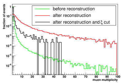
Figure 9.3: Muon multiplicity before the reconstruction (green), after the reconstruction (red) and after the reconstruction and the cut (black). The histograms have been normalised to 1.

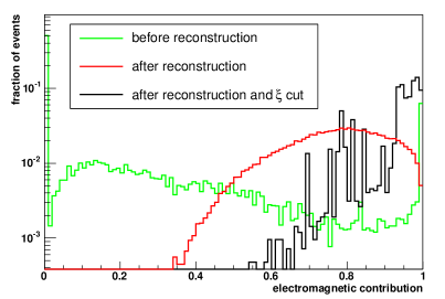
Figure 9.4: Electromagnetic contribution before the reconstruction (green), after the reconstruction (red) and after the reconstruction and the cut (black). The histograms have been normalised to 1.

9.1.2 Catastrophic Losses and Multi-Muons in the Remaining Events

To determine whether those events with large electromagnetic contributions tend to be caused by muon bundles with a large multiplicity or not, the sample of events remaining after the cut is divided into two classes: those with an electromagnetic contribution larger than 75%, and those with a smaller contribution than this value. 653 of the events remaining in the sample had an electromagnetic contribution larger than 75%; all but one of the remaining 83 events have a muon multiplicity of at least two and can therefore be considered multi-muon events. Figure 9.5 shows the muon multiplicity of the two classes of events. Again, the entries to both histograms have been weighted according to the primary proton flux, and both curves have been normalised to 1. One can see that the muon multiplicity for the events with large electromagnetic contributions is much smaller than for the other events, which leads to the conclusion that the events of the first category are indeed characterised by catastrophic losses of single muons.

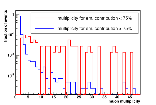
Figure 9.5: Muon multiplicity for those events with an electromagnetic contribution larger than 75% (blue) and for those with a smaller contribution (red). Both histograms have been normalised to 1.

Even though the atmospheric muon event rate has been suppressed significantly by the cut described above, it is still very high compared to the expected neutrino-induced shower rates. The following sections discusses several cuts for the differentiation between well reconstructed events and poorly reconstructed ones. It will be shown that with these cuts, also a suppression of the muon events, at least above a certain energy threshold, is possible.

9.2 Comparison of Azimuth from Calculation and Fit

An algebraic method to calculate a rough estimate of the neutrino direction was introduced in Section 7.2.1. Using the method presented there, the azimuth angle $\phi$ can be reconstructed with a RMS of $79^{\circ}$. Even though this is a poor resolution, the results of this calculation and of the fit are correlated, as can be seen from Figure 9.6: Here, the azimuth angle resulting from the fit, $\phi_{reco}$, is plotted versus the azimuth angle from the calculation, $\phi_{calc}$, for well reconstructed events (upper plot), moderately reconstructed ones (middle plot) and poorly reconstructed ones (lower plot), for event sample B. The black lines mark the regions of ${|\phi_{calc}-\phi_{reco}|<50^{\circ}}$ and ${|\phi_{calc}-\phi_{reco}|>320^{\circ}}$. The results for the well reconstructed events are correlated. The correlation between $\phi_{calc}$ and $\phi_{reco}$ weakens for the moderate events, and the majority of the poorly reconstructed events lie outside the regions marked by the black lines. Events will therefore be discarded if they do not fulfil the conditions ${|\phi_{calc}-\phi_{reco}|<50^{\circ}}$ or ${|\phi_{calc}-\phi_{reco}|>320^{\circ}}$.

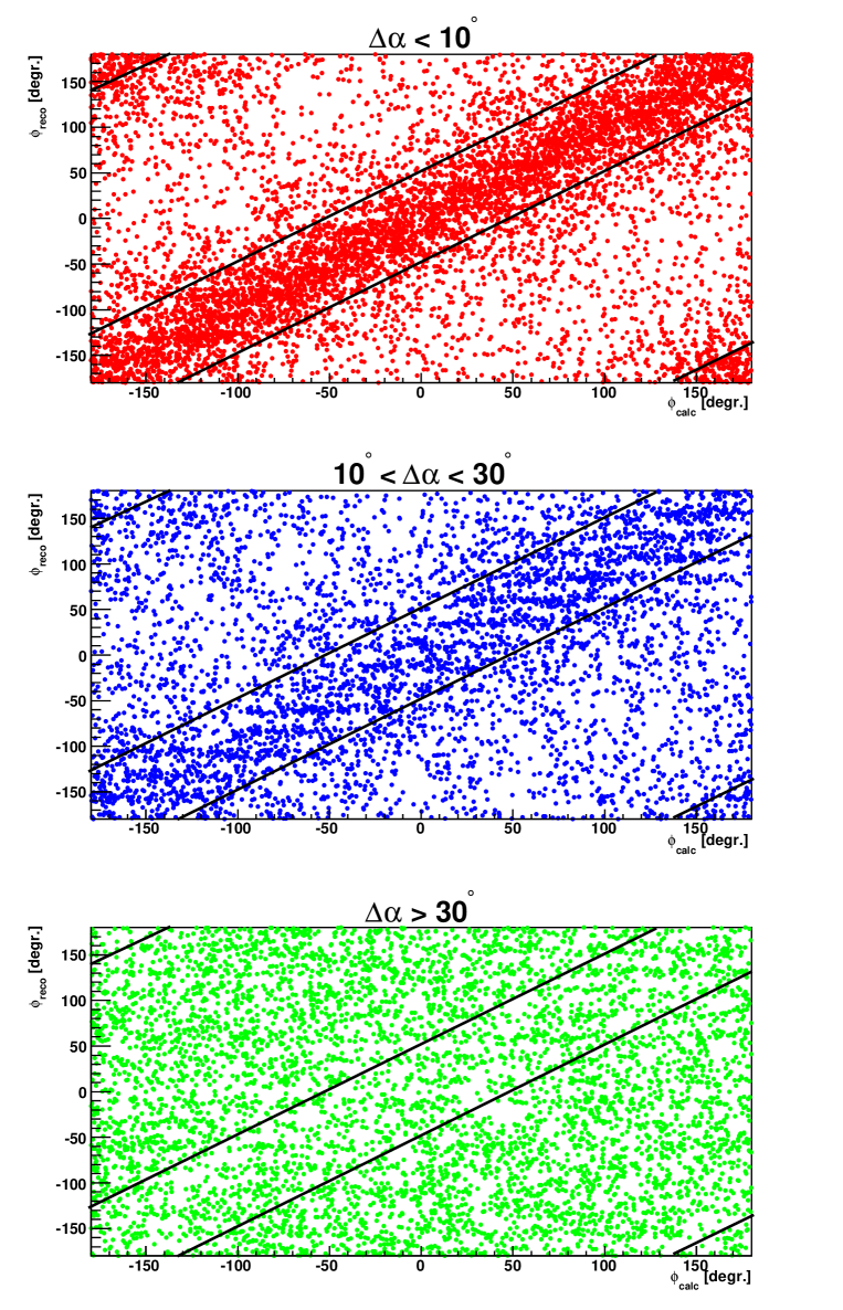
Figure 9.6: Azimuth angle obtained from the fit, $\phi_{reco}$, vs. the azimuth angle calculated as described in Section 7.2.1, $\phi_{calc}$, for well (top), moderately (middle) and poorly (bottom) reconstructed events. The region of event selection is marked by the black lines.

In principle, this cut could also be applied for the zenith angle $\theta$. However, as can be seen from Figure 7.7 in Section 7.2.1, the algebraic method tends to shift the zenith angle towards smaller angles, i.e. to an upward orientation; therefore, the correlation between $\theta_{calc}$ and $\theta_{reco}$ is not as clear as for $\phi$.
The results for the $\phi$ cut are listed in Table 9.4, in absolute numbers and in percentages with respect to the number of events after the reconstruction. The cut has a relatively high purity, as can be seen from the small percentages of poorly reconstructed events remaining in the sample. However, for the highest energy bin also the number of suppressed good events is relatively high, which is due to the fact that the calculation of the azimuth yields its best results for energies below 10 TeV, as was demonstrated in Section 7.2.1 in Figure 7.10. Due to this poor efficiency, the cut is not used for the final event selection.
Around 60% of the atmospheric muon events remaining after the cut on $\xi$ are suppressed by this cut. The numbers of atmospheric muon events in the individual bins after the different cuts are listed at the end of the chapter in Table 9.10.

NC events	good	moderate	bad	total
$E_{sh}<10$ TeV	2675 (80.6%)	1690 (66.9%)	950 (26.6%)	5315 (56.5%)
10 TeV $\leq E_{sh}<1$ PeV	2275 (55.7%)	570 (27.0%)	326 (16.8%)	3171 (39.0%)
$E_{sh}\geq 1$ PeV	110 (28.8%)	10 (6.58%)	32 (22.2%)	152 (22.4%)
total	5060 (65.0%)	2270 (47.4%)	1308 (23.1%)	8638 (47.4%)

$\nu_{e}$ CC events	good	moderate	bad	total
$E_{sh}<10$ TeV	4921 (79.4%)	2690 (64.9%)	1795 (28.4%)	9406 (56.4%)
10 TeV $\leq E_{sh}<1$ PeV	3120 (50.9%)	656 (21.1%)	471 (17.1%)	4247 (35.4%)
$E_{sh}\geq 1$ PeV	349 (23.6%)	40 (7.65%)	68 (13.7%)	457 (18.3%)
total	8390 (60.7%)	3386 (43.6%)	2334 (24.4%)	14110 (45.3%)

Table 9.4: Number of good, moderate and bad events in the three energy bins, after the cut on $|\phi_{p}-\phi_{f}|$. The percentages were calculated with respect to the number of events after the reconstruction, as displayed in Table 9.1.

9.3 Comparison of Energy from Calculation and Fit

For the energy, an analogous method to that introduced above in Section 9.2 can be applied. In Section 7.3, an algorithm was described to reconstruct the shower energy to a factor of about $2.3$ (for WF mode). This method assumes that all photons are emitted under a fixed angle and uses the position and direction of the shower, calculated according to the descriptions in Sections 7.1 and 7.2.1.
The parameterisation of the angular photon distribution $D(\vartheta)$ is not used for the calculation. Therefore the calculated energy is not directly correlated to the result from the likelihood minimisation (though the same values for the shower position are used), and thus, a comparison between the reconstructed energy from the fit, $E_{reco}$, and the energy from the calculation, $E_{calc}$, can be used to assess the consistency of the results. The correlation between $E_{calc}$ and $E_{reco}$ is shown in Figure 9.7, for the NC event sample B. Events pass the cut if they lie within the region marked by the two bold lines, i.e. if the difference between $\log_{10}E_{calc}$ and $\log_{10}E_{reco}$ is not larger than 0.6.

The events remaining in the sample after this cut are listed in Table 9.5. The percentages given refer to the number of events that remained in the sample after the reconstruction, as given in Table 9.1. The efficiency of this cut is high. It was therefore selected as one of the final cuts on the event samples.
For the muon suppression, this cut is almost as effective as the cut on the azimuth angles introduced in the previous section. About 51% of the atmospheric muons remaining in the sample after the cut on $\xi$ are suppressed by this cut. Detailed numbers are given in Table 9.10.

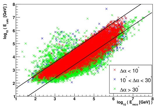
Figure 9.7: $E_{calc}$ vs. $E_{reco}$ for good, moderate and bad events, and the cut conditions (bold lines).

NC events	good	moderate	bad	total
$E_{sh}<10$ TeV	3197 (96.4%)	2219 (87.8%)	2224 (62.3%)	7640 (81.2%)
10 TeV $\leq E_{sh}<1$ PeV	3349 (82.0%)	1072 (50.7%)	817 (42.0%)	5238 (64.4%)
$E_{sh}\geq 1$ PeV	277 (72.5%)	69 (45.4%)	91 (63.2%)	437 (64.5%)
total	6823 (87.8%)	3360 (70.1%)	3132 (55.4%)	13315 (73.0%)

$\nu_{e}$ CC events	good	moderate	bad	total
$E_{sh}<10$ TeV	5982 (96.5%)	3599 (86.8%)	4078 (64.6%)	13659 (82.0%)
10 TeV $\leq E_{sh}<1$ PeV	4896 (79.8%)	1425 (45.9%)	1155 (41.9%)	7476 (62.3%)
$E_{sh}\geq 1$ PeV	1113 (75.2%)	244 (46.7%)	288 (58.2%)	1645 (65.9%)
total	11991 (86.8%)	5268 (67.8%)	5521 (57.7%)	22780 (73.1%)

Table 9.5: Number of good, moderate and bad events in the three energy bins, after the cut on $|\log_{10}(E_{calc}/E_{reco})|$. The percentages were calculated with respect to the number of events after the reconstruction, as displayed in Table 9.1.

9.4 Large Energies

Due to the larger total number of hits and the larger hit amplitudes, the pattern matching algorithm improves for energies in the TeV region or higher. Also, the suppression of the optical background shows the best efficiency at high energies; and finally, the atmospheric muon background decreases significantly if only high-energy events are considered. Therefore, a cut is proposed at a minimum reconstructed shower energy of 5 TeV.
The results of this cut are shown in Table 9.6. As expected, nearly all events with a true shower energy above 10 TeV pass the cut. Most of the events remaining in the lowest energy bin have true shower energies above 5 TeV, though there are a few misreconstructed events with lower true energies which pass the cut (see Figures 9.9 and 9.10 at the end of the chapter).

NC events	good	moderate	bad	total
$E_{sh}<10$ TeV	964 (29.1%)	603 (23.9%)	1155 (32.4%)	2722 (28.9%)
10 TeV $\leq E_{sh}<1$ PeV	4071 (99.7%)	2046 (96.8%)	1655 (85.2%)	7772 (95.5%)
$E_{sh}\geq 1$ PeV	382 (100%)	150 (98.7%)	140 (97.2%)	672 (99.1%)
total	5417 (69.6%)	2799 (58.4%)	2950 (52.2%)	11166 (61.3%)

$\nu_{e}$ CC events	good	moderate	bad	total
$E_{sh}<10$ TeV	2009 (32.4%)	991 (23.9%)	1827 (28.9%)	4827 (29.0%)
10 TeV $\leq E_{sh}<1$ PeV	6113 (99.6%)	3037 (97.9%)	2360 (85.5%)	11510 (95.9%)
$E_{sh}\geq 1$ PeV	1479 (99.9%)	519 (99.2%)	490 (99.0%)	2488 (99.6%)
total	9601 (69.5%)	4547 (58.5%)	4677 (48.9%)	18825 (60.4%)

Table 9.6: Number of good, moderate and bad events in the three energy bins, after the cut on $E_{reco}>5$ TeV. The percentages were calculated with respect to the number of events after the reconstruction, as displayed in Table 9.1.

9.5 Upgoing Events

For energy regions where the atmospheric muon background cannot be suppressed sufficiently by the cut on $\xi$ described above, it is necessary to consider only events which have been reconstructed as upgoing. As the photomultipliers in the ANTARES experiment look downwards, the resolution for events from above is generally worse than for those from below. However, because of the photomultiplier orientation, the event vertices tend to be reconstructed too high, i.e. with a too large $z$ coordinate (see Figure 7.2 in Section 7.1). In such cases, a downgoing direction is favoured in the pattern matching. Events with a large positional error are therefore often reconstructed as downgoing. $12\%$ of the upgoing, but only $5\%$ of the downgoing events were reconstructed with a wrong orientation, i.e. downgoing instead of upgoing or vice-versa.
The results of selecting only events which have been reconstructed as upgoing from the shower event samples are listed in Table 9.7. As the primary neutrinos were generated isotropically in $4\pi$, one can see that up to 1 PeV the upgoing events are reconstructed more efficiently than the downgoing ones: The percentage of remaining good or moderate events is larger than that of the remaining bad events.
Considering the atmospheric muon sample, it turns out that 18% of the events remaining in the sample after the muon reconstruction are reconstructed as upgoing by the shower reconstruction strategy (see Table 9.10). Therefore, even if only upgoing events are studied, the background contamination is still considerably high, at least below $\sim 5$ TeV, as will be shown in Chapter 10. Furthermore, the advantage of neutrino-induced showers to be able to study downgoing events, would be lost by such a cut.

NC events	good	moderate	bad	total
$E_{sh}<10$ TeV	2182 (65.8%)	1463 (57.9%)	1696 (47.5%)	5341 (56.7%)
10 TeV $\leq E_{sh}<1$ PeV	2351 (57.6%)	927 (43.9%)	768 (39.5%)	4046 (49.7%)
$E_{sh}\geq 1$ PeV	187 (49.0%)	69 (45.4%)	68 (47.2%)	324 (47.8%)
total	4720 (60.7%)	2459 (51.3%)	2532 (44.8%)	9711 (53.3%)

$\nu_{e}$ CC events	good	moderate	bad	total
$E_{sh}<10$ TeV	4143 (66.8%)	2410 (58.1%)	3054 (48.3%)	9607 (57.6%)
10 TeV $\leq E_{sh}<1$ PeV	3515 (57.3%)	1348 (43.4%)	1128 (40.9%)	5991 (49.9%)
$E_{sh}\geq 1$ PeV	700 (47.3%)	255 (48.8%)	240 (48.5%)	1195 (47.8%)
total	8358 (60.5%)	4013 (51.6%)	4422 (46.2%)	16793 (53.9%)

Table 9.7: Number of good, moderate and bad events in the three energy bins, after checking if the neutrino was reconstructed as upgoing. The percentages were calculated with respect to the number of events after the reconstruction, as displayed in Table 9.1.

9.6 Cuts Based on Geometrical Considerations

In this section, the results on studies of the suppression of poorly reconstructed events by selecting events by their position and direction with respect to the instrumented volume are presented. Even though events with an interaction vertex outside the detector, or events pointing to the outside of the detector, are generally more difficult to reconstruct, there are actually a lot of events which show very satisfying results. It turns out that, attempting to suppress events which are geometrically unfavourable for the reconstruction, also a large fraction of well reconstructed events are rejected. A reason for this is that, due to the usage of the filter conditions on all events (see Chapter 6.4), those events which really produce only a small signal, because of their disadvantageous position and direction with respect to the detector, are not considered for the reconstruction in the first place.
In the following two subsections, selection criteria for geometrically unfavourable events are introduced. Due to the unsatisfying efficiency of these cuts, none of them were used in the final event selection.

9.6.1 Events Leaving the Instrumented Volume

As has been discussed in Section 8.2.3, the conditions for a successful reconstruction are fulfilled if the shower is contained inside the instrumented volume of the detector or points right into it. A means to check for these geometrical criteria in an event is to verify whether a point at a distance $d$ from the reconstructed position $X$, along the reconstructed direction $\vec{v}$, lies a can of selectable size around the instrumented volume. The principle of this selection criterion is demonstrated in Figure 9.8: The can inside which the point must lie is marked in black, the instrumented volume in light blue: Event 1 in green fulfils the criterion, while event 2 in red does not.

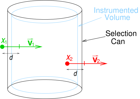
Figure 9.8: Geometrical principle of the cut on events leaving the detector. The green event labelled 1 is accepted, while the red one labelled 2 is rejected.

The results of this cut, for a chosen distance $d=20$ m and a can which extends 10 m beyond the instrumented volume, are shown in Table 9.8. For the chosen sizes of $d$ and the can, the efficiency of this cut is still above 50% for the good events, but on the other hand, also half of the poorly reconstructed events remains in the sample. This number could be decreased by decreasing the selected can size, but that would consequently also lead to a stronger suppression of the well reconstructed events and is therefore not favourable.

NC events	good	moderate	bad	total
$E_{sh}<10$ TeV	2785 (83.9%)	2098 (83.0%)	2276 (63.8%)	7159 (76.1%)
10 TeV $\leq E_{sh}<1$ PeV	2391 (58.6%)	808 (38.2%)	751 (38.7%)	3950 (48.5%)
$E_{sh}\geq 1$ PeV	205 (53.7%)	34 (22.4%)	64 (44.4%)	303 (44.7%)
total	5381 (69.1%)	2940 (61.4%)	3091 (54.7%)	11412 (62.6%)

$\nu_{e}$ CC events	good	moderate	bad	total
$E_{sh}<10$ TeV	5162 (83.3%)	3437 (82.9%)	4164 (65.9%)	12763 (76.6%)
10 TeV $\leq E_{sh}<1$ PeV	3488 (56.9%)	1076 (34.7%)	974 (35.3%)	5538 (46.2%)
$E_{sh}\geq 1$ PeV	714 (48.2%)	138 (26.4%)	195 (39.4%)	1047 (41.9%)
total	9364 (67.8%)	4651 (59.8%)	5333 (55.7%)	19348 (62.1%)

Table 9.8: Number of good, moderate and bad events in the three energy bins, after the cut on the pointing direction of the reconstructed shower. The percentages were calculated with respect to the number of events after the reconstruction, as displayed in Table 9.1.

9.6.2 Events Inside the Instrumented Volume

A method that is very similar to the one described in the previous subsection is to check if the reconstructed position of an event lies within the instrumented volume, i.e. if the event is contained. An event passes this cut if its radial distance from the centre of the detector is smaller than 100 m, and if its vertical distance to the horizontal plane through the detector centre is less than 175 m.
As this method does not check for the direction of the shower, it is less efficient than the one introduced above; also the purity is lower (see plots at the end of the chapter).
The results of the cut on contained events can be seen from Table 9.9.

NC events	good	moderate	bad	total
$E_{sh}<10$ TeV	2369 (71.4%)	1831 (72.5%)	2173 (60.9%)	6373 (67.7%)
10 TeV $\leq E_{sh}<1$ PeV	1978 (48.5%)	741 (35.1%)	686 (35.3%)	3405 (41.8%)
$E_{sh}\geq 1$ PeV	174 (45.5%)	28 (18.4%)	59 (41.0%)	261 (38.5%)
total	4521 (58.1%)	2600 (54.3%)	2918 (51.6%)	10039 (55.1%)

$\nu_{e}$ CC events	good	moderate	bad	total
$E_{sh}<10$ TeV	4346 (70.1%)	2959 (71.3%)	3936 (62.3%)	11241 (67.4%)
10 TeV $\leq E_{sh}<1$ PeV	2845 (46.4%)	999 (32.2%)	903 (32.7%)	4747 (39.6%)
$E_{sh}\geq 1$ PeV	603 (40.7%)	114 (21.8%)	177 (35.8%)	894 (35.8%)
total	7794 (56.4%)	4072 (52.4%)	5016 (52.4%)	16882 (54.2%)

Table 9.9: Number of good, moderate and bad events in the three energy bins, after the cut on containment. The percentages were calculated with respect to the number of events after the reconstruction, as displayed in Table 9.1.

9.7 Efficiencies and Purities of the Cuts

The quality of a cut depends on two factors: How many of the good events remain in the sample after the cut, and how many of the bad events are removed. The efficiency $\mathcal{E}$ of a cut is defined as the ratio between the number of good events after the cut, $n^{good}_{c}$, and the number of good events before the cut, $n^{good}$:

$$\mathcal{E} = \frac{n^{good}_{c}}{n^{good}}.$$

The purity $\mathcal{P}$, on the other hand, is defined as the number of good events after the cut, $n^{good}_{c}$, divided by the total number of events after the cut, $n_{c}$:

$$\mathcal{P} = \frac{n^{good}_{c}}{n_{c}}.$$

For the plots shown in the following, a good event is defined as described at the beginning of this chapter: an event reconstructed with a total angular error smaller than $10^{\circ}$. For this discussion, only good, and not also the moderate events, contribute to a high efficiency and purity, as those events with a small angular error below $10^{\circ}$ are of the primary importance for the analysis.
For the sample of NC events that was used in this chapter, event sample B, the efficiencies and purities for the different cuts are given in Figure 9.9, together with the statistical errors (see appendix C.1 for details on the error calculation). The efficiencies and purities of the cuts applied to the $\nu_{e}$ CC sample are shown in Figure 9.10. For the analysis of measured shower events, which will consist of both types of shower events without a possibility to distinguish between them, the chosen cuts should be effective on both data samples. All cuts have a very similar effect both to NC and $\nu_{e}$ CC events, as can be seen from the figures.
Apart from the cut on $\xi$ (see Section 9.1.1), which suppresses the atmospheric muon background very efficiently, it was decided to use the cut on the energy comparison (see Section 9.3), because it shows a very high efficiency throughout the whole energy range, combined with a satisfying purity which exceeds 50% above $\sim 5$ TeV. As the energy region above 5 TeV is the region of main interest, it is also advisable to restrain on events with a reconstructed energy above 5 TeV, as proposed in Section 9.4. The combined efficiency and purity of these three cuts are displayed in Figure 9.11 for NC events, and in Figure 9.12 for $\nu_{e}$ CC events. The low energy region has been omitted for these plots.

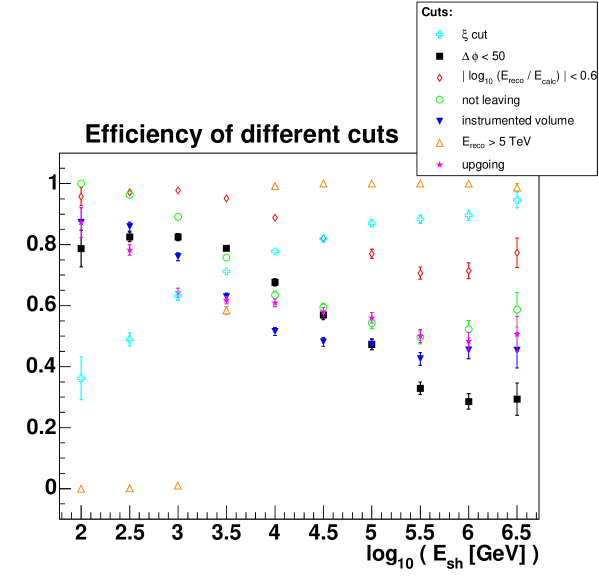
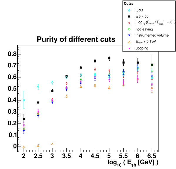
Figure 9.9: Efficiency (top) and purity (bottom) of the cuts described in the text, for the NC sample.

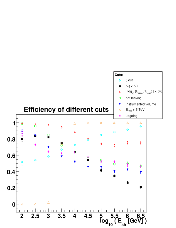
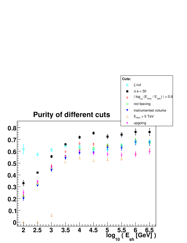
Figure 9.10: Efficiency (top) and purity (bottom) of the cuts described in the text, for the $\nu_{e}$ CC sample.

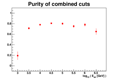
Figure 9.11: Combined efficiency (left) and purity (right) of the selected cuts (see text), for the NC sample.

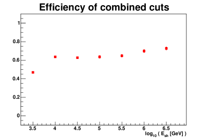
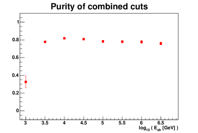
Figure 9.12: Combined efficiency (left) and purity (right) of the selected cuts (see text), for the $\nu_{e}$ CC sample.

Table 9.10 lists the numbers of events remaining in the different bins of the atmospheric muon sample after the cuts described above. The event rates after some of the cuts will be presented in the next chapter, together with the respective neutrino rates, in Figure 10.13 in Section 10.4.

angle	$0^{\circ}-60^{\circ}$
primary energy [TeV/nucleon]	1-10	10-100	100-105
$|\Delta\phi<50^{\circ}|$	3 (27.3%)	11 (34.4%)	178 (37.7%)
$|\log_{10}(E_{calc}/E_{reco})|<0.6$	5 (45.5%)	14 (43.8%)	223 (47.2%)
$E_{reco}>5$ TeV	0 (0%)	6 (18.75%)	127 (26.9%)
upgoing	2 (18.2%)	4 (12.5%)	73 (15.5%)
not leaving	11 (100%)	28 (87.5%)	357 (75.6%)
instrumented volume	10 (90.9%)	27 (84.3%)	330 (69.9%)

angle	$60^{\circ}-85^{\circ}$
primary energy [TeV/nucleon]	1-10 ∗	10-100	100-105
$|\Delta\phi<50^{\circ}|$	0 ∗	1 (33.3%)	95 (43.6%)
$|\log_{10}(E_{calc}/E_{reco})|<0.6$	0 ∗	1 (33.3%)	132 (60.6%)
$E_{reco}>5$ TeV	0 ∗	0 (0%)	33 (15.1%)
upgoing	0 ∗	2 (66.7%)	42 (19.3%)
not leaving	0 ∗	2 (66.7%)	178 (81.7%)
instrumented volume	0 ∗	2 (66.7%)	164 (75.2%)

Table 9.10: Numbers of events in the different energy and angular bins of the atmospheric muon event sample, after the cuts described in Sections 9.2 to 9.6.2. The percentages were calculated with respect to the number of events after the cut on $\xi$, as displayed in Table 9.3. The lowest energy horizontal bin, marked with an asterisk, contained zero events after the cut on $\xi$.

Chapter 10 Results of the Reconstruction

In this chapter, the results for the reconstruction of different shower-type event samples are presented. The results are based on the assumption that the saturation in the photomultiplier electronics is reached at 200 pe, i.e. that data are taken in WF mode, except for the results presented in Section 10.1.1, which were obtained under the assumption of data taking in SPE mode. In the first section, Section 10.1, results for the reconstruction of NC events are presented; results for the reconstruction of $\nu_{e}$ CC events follow in Section 10.2. The results are shown after the cut on a reconstructed shower energy $>5$ TeV (see Section 9.4), and after the additional cuts on the variable $\xi$ comparing expected and measured hit amplitudes (see Section 9.1.1) and on the comparison between reconstructed and calculated energy (see Section 9.3).
Sections 10.3 and 10.4 show the effective areas obtained with the reconstruction algorithm presented in this thesis, together with calculations of the sensitivity of the ANTARES experiment to the diffuse cosmic neutrino fluxes, using neutrino-induced showers.

10.1 Reconstruction of NC Events

The results shown in this section were obtained reconstructing event sample B which contains 140000 NC events (see Appendix A.5.1 for details). Some 18000 events remain in the sample after the reconstruction. In Figures 10.1 and 10.2, results after the appliance of the cut selecting events with a reconstructed shower energy above 5 TeV are shown. Figure 10.1 shows the total angular error $\Delta\alpha$ between the neutrino direction and the reconstructed direction, in degrees, on the left hand side for all energies, and on the right hand side the median of $\Delta\alpha$ for different bins in the MC shower energy.
In Figure 10.2 the distribution of the logarithmic error on the reconstructed shower energy is shown on the left hand side, and the distribution of the logarithmic error on the neutrino energy is shown on the right. As the fraction of the primary neutrino energy which is transferred into the hadronic shower is not known, only a lower limit can be given for the reconstructed neutrino energy (see comments in Section 8.2.2). The RMS of the logarithmic error on the shower energy corresponds to a factor ${10^{0.4}\approx 2.5}$ between the reconstructed and the true shower energy, though the peak is narrower, with a width of $\sim 0.17$, obtained from the Gaussian fit marked by the red line in Figure 10.2. This width corresponds to a factor of 1.5. The RMS of the logarithmic error on the shower energy, calculated within different MC energy regions, is displayed in Figure 10.3.

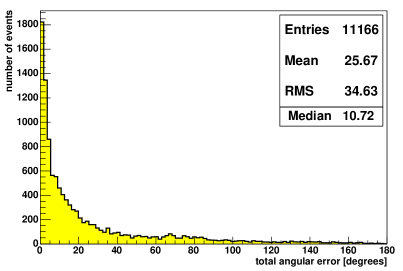
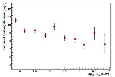
Figure 10.1: Total angular error $\Delta\alpha$ between neutrino and reconstructed direction, after the cut on $E_{reco}>5$ TeV: Distribution for all energies (left), and median of total angular error for different MC shower energy bins (right). The error bars mark the statistical standard errors whose calculation is described in Appendix C.2.

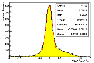
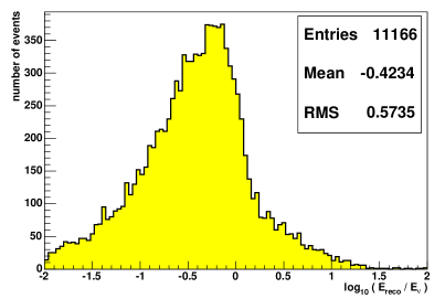
Figure 10.2: Distribution of the logarithmic difference between reconstructed energy and MC shower energy (left), and between reconstructed energy and neutrino energy (right), after the cut on $E_{reco}>5$ TeV. A Gaussian distribution shown in red has been fitted to the peak of the shower energy error.

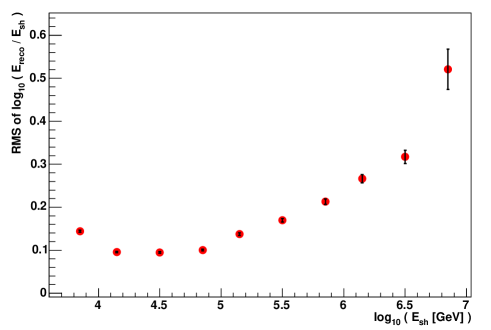
Figure 10.3: RMS of the logarithmic error on the shower energy, for different bins in the MC shower energy, after the cut on $E_{reco}>5$ TeV.

In addition to the cut on the reconstructed shower energy, two more cuts were chosen according to their efficiencies and the purities, one cutting on a variable $\xi$ (see Section 9.1.1) and one on a comparison between reconstructed and calculated shower energy (see Section 9.3). 43% of the events passing the reconstruction and having a reconstructed shower energy $>5$ TeV survive these additional cuts. The results for the error on direction and energy after these cuts are shown in figures 10.4 and 10.5. Both the angular and the energy resolution have improved significantly, from a median of $10.7^{\circ}$ to $3.5^{\circ}$ in the direction, with values of about $2^{\circ}$ around 100 TeV (see right plot of Figure 10.4), and an improvement from 0.40 to 0.20 in the RMS of the logarithmic shower energy resolution. The peak of this distribution has a width of 0.14, which means a resolution correspoding to a factor of $1.4$.

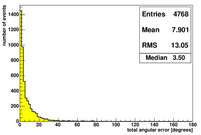
Figure 10.4: Total angular error between neutrino and reconstructed direction for all energies (left), and median of total angular error for different MC shower energy bins (right), with statistical errors, after all three cuts.

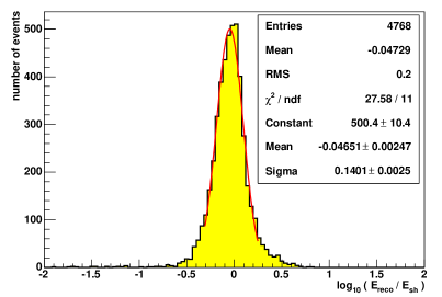
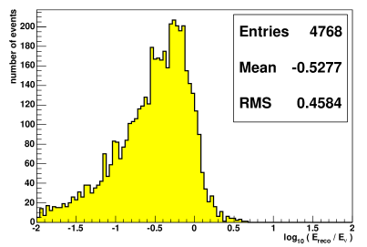
Figure 10.5: Distribution of the logarithmic error between reconstructed energy and MC shower energy (left), and between reconstructed energy and neutrino energy (right), after all three cuts.

10.1.1 Results for SPE Mode

The default value for the saturation of the photomultiplier electronics in the ShowerFitter is the value of the WF mode, 200 pe. However, as discussed in Section 4.3.1, data taken in the WF mode need forty times more bandwidth and storage capacity than in the SPE mode, which has a saturation at 20 pe. It is therefore not sure if the ANTARES detector will take a large number of runs in the WF mode. The effect of a lower saturation level has therefore been examined using the smaller NC event sample A. Note that in comparison to event sample B, this sample contains only events with interaction vertices inside the instrumented volume, and is therefore expected to produce better results in the reconstruction than event sample B.
Event sample A has been reconstructed twice, once in WF mode and once in SPE mode. As the main principle of the fit is the matching of measured and calculated amplitudes, it is expected that the results deteriorate when the saturation level is set to a smaller value, since this means an information loss.
Shown as results for the SPE mode are the total angular error $\Delta\alpha$ in Figure 10.6, for all energies (left), and the median of $\Delta\alpha$ for the different energy bins (right). The total number of reconstructed events is smaller than the number of the reconstructed events in the WF mode, 2767 compared to 2908 events. This is mainly caused by failures of the fit for high-energy events in the SPE mode, if no satisfying result is found in the minimisation. The results for the reconstruction of the same sample using the WF mode are shown as the red lines on the left, and as red stars on the right of Figure 10.6. For shower energies below $\sim 70$ TeV, the resolution for the SPE mode is even slightly better than for the WF mode, because the statistical fluctuations in the photon distributions which occur at these smaller energies are damped by lower amplitude saturation. For higher energies, the resolution for the SPE mode deteriorates, but not much. For the WF mode, a deterioration of the resolution due to the saturation effects is observed as well, but starting at higher energies.
For the reconstruction of the shower energy, the resolution is equivalent in WF and SPE mode, see left plot of Figure 10.7; the distribution obtained in SPE mode is shifted to energies reconstructed too low, as expected for a lower saturation (note that the calculation of the shower energy from the number of photo-electrons in an event was optimised for the WF mode). The reconstructed neutrino energy shows deteriorations only slightly, see right plot in the same figure.
From this comparison, it can be concluded that, even though the saturation level is significantly smaller for the SPE mode, the deterioration of the resolution is not large. A good reconstruction of shower events is therefore possible also for data taken in the SPE mode.

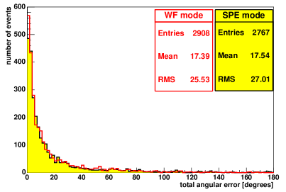
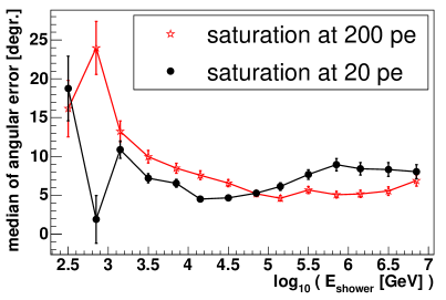
Figure 10.6: Total angular error between neutrino and reconstructed direction, for all energies (left), and median of total angular error for different MC shower energy bins (right), with statistical errors, before all cuts, for SPE and WF mode. On the left plot, the events from WF mode are drawn with a red line, as is their statistics, while the events from SPE mode are represented by the yellow histogram.

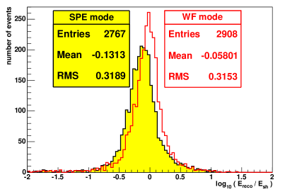
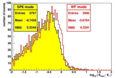
Figure 10.7: Distribution of logarithmic error between reconstructed energy and MC shower energy (left), and between reconstructed energy and neutrino energy (right), before all cuts, for SPE and WF mode. The events obtained in WF mode are drawn in red, those obtained in SPE mode are filled in yellow. The offset for the SPE mode in the left plot is caused by the fact that the calculation of the shower energy from the photon number is optimised for the WF mode.

10.2 Reconstruction of $\nu_{e}$ CC events

In principle, the event topology of $\nu_{e}$ CC events is different to that of NC events, because of the higher electromagnetic contribution (see Section 5.2). However, the electromagnetic component of a hadronic shower grows with increasing shower energy and exceeds 90% already at 1 TeV (cf. Section 5.3). Therefore, a large amount of photons and electrons is present in NC events, and additionally, $\nu_{e}$ CC events are always accompanied by a hadronic shower. Thus it is well possible to reconstruct NC and $\nu_{e}$ CC events with the same reconstruction strategy. In a sparsely instrumented detector like ANTARES, it will most probably not be possible to distinguish between the two event types, because of their similar topologies.
The crucial difference between the two event types is in the energy reconstruction. While in NC events a (mostly larger) part of the energy of the primary neutrino is carried away unseen by the outgoing neutrino, in $\nu_{e}$ CC events all energy goes into showers and can therefore be detected. It is therefore expected that for these events the resolution of the neutrino energy reconstruction is much better than for NC events.
In the following, results for a sample of 138500 $\nu_{e}$ CC events are shown. The energy and angular distributions of the primary neutrinos are the same as in the NC sample. The $\nu_{e}$ CC data sample is described in more detail in Appendix A.5.2.
The results obtained are very similar to those shown for the NC sample. The overall angular resolution $\Delta\alpha$ after the cut on $E_{reco}>5$ TeV, as shown in Figure 10.8, has a median of $9.5^{\circ}$, almost the same as for the NC sample shown in Figure 10.1, where the median is $10.7^{\circ}$. It should be noted that due to the kinematics, the $\nu_{e}$ CC events are a factor of 2 – 3 more energetic than the NC events, with respect to the shower energy, and therefore the contribution of lower energy events in the sample is smaller than for the NC events, which leads to a slight overall improvement of the results.
Figure 10.9 shows the resolution of the shower energy, which in this case is equivalent to the neutrino energy, after the cut on $E_{reco}>5$ TeV, on the left hand side. The RMS of the distribution is 0.41, with a width of 0.19 in the Gaussian fitted peak. This width corresponds to a factor of 1.5 in the energy resolution, which is again very similar to that of the NC events shown in Figure 10.2 (left).
The same additional two cuts that were applied to the NC sample above (see Section 9.1.1 and Section 9.3) were also applied to this sample. 37% of the events which have passed the reconstruction and the cut on the reconstructed shower energy remain after these cuts. The right hand side of Figure 10.9 shows the energy resolution after the cuts. The RMS has improved from 0.41 to 0.21 with a width of the peak of around 0.16, which corresponds to a factor of ${1.4}$ in the energy reconstruction. The result for the total angular resolution after the cuts is shown in Figure 10.10. The overall median has improved to $3.0^{\circ}$, and the best resolution, reached at about $100$ TeV, is below $2^{\circ}$.

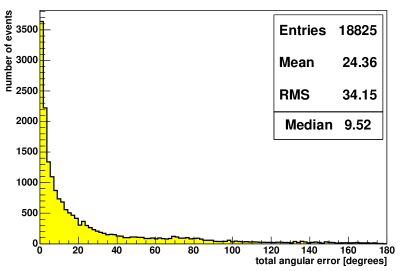
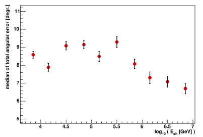
Figure 10.8: Total angular error between neutrino and reconstructed direction, for all energies (left), and median of total angular error for different MC shower energy bins, with statistical errors (right), after the cut on the reconstructed shower energy, for $\nu_{e}$ CC events.

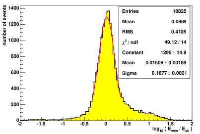
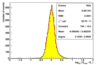
Figure 10.9: Logarithmic error between reconstructed and MC shower (=neutrino) energy for $\nu_{e}$ CC events, after the cut on the reconstructed shower energy (left), and after the additional two cuts (right).

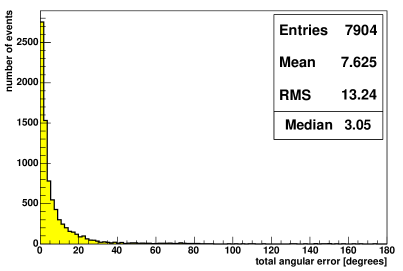
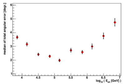
Figure 10.10: Total angular error between neutrino and reconstructed direction,for all energies (left), and median of total angular error for different MC shower energy bins (right), with statistical errors, after the cuts.

It can therefore be concluded that the reconstruction algorithm presented in this thesis is suitable both for NC and for $\nu_{e}$ CC events, which is of extreme importance for its applicability to real data, because a distinction between the two event types may not be possible. From these results the expected resolution for a shower-type event after the shown cuts is about $3^{\circ}$–$4^{\circ}$, with an energy resolution corresponding to a factor of 1.4.

10.3 Effective Volume and Effective Neutrino Area

To give an estimate on the sensitivity of the ANTARES experiment to cosmic neutrino flux, the effective volume and effective neutrino area of the detector are determined as described in Section 3.3.1.
Figure 10.11 shows the results for the NC sample. The figure shows effective volume (left) and effective area (right) over the MC neutrino energy, after the reconstruction (black line) and after the three cuts (red line, see Sections 9.1.1, 9.3 and 9.4). Before the cuts, the effective area corresponds roughly to 1/10th of the effective muon neutrino area reached for $\nu_{\mu}$ CC events without cuts [Bai01].

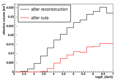
Figure 10.11: Effective volume (left) and effective neutrino area (right) for the reconstruction of NC events presented in Section 10.1, after the reconstruction (black) and the cuts (red).

In Figure 10.12, the effective volume (left) and effective area (right) for the $\nu_{e}$ CC events are shown. Results for these events were presented in Section 10.2. The colour coding is the same as for Figure 10.11. Above 100 TeV, the effective volume before the cuts reaches a plateau which corresponds to the generation volume of the events, pointing at the fact that practically all events above this energy pass the reconstruction. The values of effective volume and effective area after the cuts are slightly larger than those reached for the NC events, as the showers induced in $\nu_{e}$ CC events are more energetic with respect to the neutrino energy, and therefore more likely to pass the reconstruction.

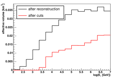
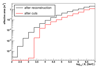
Figure 10.12: Effective volume (left) and effective neutrino area (right) for the reconstruction of $\nu_{e}$ CC events presented in Section 10.2, after the reconstruction (black) and the cuts (red).

10.4 Predictions on Rates and Diffuse Flux Sensitivity

Expected rates of shower-type events for the ANTARES detector have been estimated from the events remaining in the NC sample B and the $\nu_{e}$ CC sample after the reconstruction and the cuts. For the cosmic neutrino event rate, a hypothetical flux corresponding to the Waxman-Bahcall limit [Bah99] was assumed:

$$E_{\nu}^{2}\Phi_{cosmic}=4.5\times 10^{-8}\,\textrm{GeV s}^{-1}\,\textrm{sr}^{-1}\,\textrm{cm}^{-2}.$$ (10.1)

It was assumed that, due to oscillations, the cosmic neutrino ratio at Earth is the same for all flavours, $\nu_{e}:\nu_{\mu}:\nu_{\tau}=1:1:1$. As the event rates for the NC sample correspond to one of six possible channels of the type

$$(\nu_{l},\bar{\nu}_{l})+N\to(\nu_{l},\bar{\nu}_{l})+\textrm{hadronic shower},$$

the rates for the sample were multiplied by six to retrieve the event rates for all-flavour NC interactions, assuming identical cross sections for anti-neutrinos and neutrinos. This simplification leads to an overestimation of the rates of $\sim 18\%$ at 50 TeV, decreasing to almost zero for 1 PeV where the cross sections can be regarded as identical (see Section 3.1). Likewise, the rates retrieved for the cosmic neutrinos from the $\nu_{e}$ CC sample were multiplied by two to take into account the $\bar{\nu}_{e}$ CC channel as well. Here, the assumption of identical cross sections for electron neutrinos and anti-neutrinos leads to an overestimation of $\sim 10\%$ at 50 TeV which decreases to almost zero for energies above 300 TeV. Note that the Glashow resonance for the $\bar{\nu}_{e}$ CC channel at 6.3 PeV, which causes an increase of the cross section at the resonance energy, was not taken into account here.
For the atmospheric neutrino background, it was assumed that no tau neutrinos occur. Shower events can then be induced by muon neutrinos in a NC interaction, or by electron neutrinos in a NC or CC interaction. To estimate the total rate for NC interactions, the muon neutrino rate was calculated from the event weights for atmospheric neutrinos in event sample B (see Appendix A.5.1); those event weights were calculated during the production according to the Bartol flux [Agr96]. The expected rate for atmospheric electron neutrinos was calculated estimating that the rate of atmospheric electron neutrinos is 16 times smaller than that of atmospheric muon neutrinos for energies below 10 TeV and identical to the atmospheric muon neutrino rate above 1 PeV (see e.g. Figure 10.16); in between, the difference $\Delta\Phi_{\nu_{\mu}:\nu_{e}}$ between the two fluxes was parameterised as

$$\log_{10}\Delta\Phi_{\nu_{\mu}:\nu_{e}}=-0.45\cdot\log_{10}E_{\nu}/{\textrm{GeV}}+2.7,\quad 10^{4}\,{\textrm{GeV}}\leq E_{\nu}\leq 10^{6}\,{\textrm{GeV}}$$ (10.2)

To this approximated rate for NC events, the rate for $\nu_{e}$ CC had to be added. The results from the $\nu_{e}$ CC event sample (see Appendix A.5.2) were used for this. As for the cosmic neutrinos, the rates were again considered to be the same for neutrinos and anti-neutrinos.
The rates thus determined can be considered as the total expected rates for shower-type events from atmospheric and cosmic neutrinos in ANTARES. The resulting rates per year after reconstruction and cuts are plotted for isotropic fluxes in Figure 10.13, vs. the reconstructed energy. The cosmic neutrino rates exceeds the atmospheric neutrino rate above $\sim 50$ TeV.
The rate of atmospheric muons, again versus the reconstructed energy, is shown in blue, after the cuts which were also applied to the neutrino samples. The rate drops to zero above $\sim 20$ TeV, since no events remain in the sample above this energy. This may be due to statistics; note, however, that especially the high-energy atmospheric muons are very strongly suppressed by the cut on $\xi$ (see Figure 9.2). Nevertheless, the atmospheric muon rate may be underestimated.
In Figure 10.14, the rates for events which were reconstructed as upgoing are shown. For the selected energy region of $E_{reco}>5$ TeV, the neutrino flux exceeds the atmospheric muon flux in all energy bins shown. It can therefore be concluded that a reliable detection of neutrino-induced shower events will be possible in this energy region.

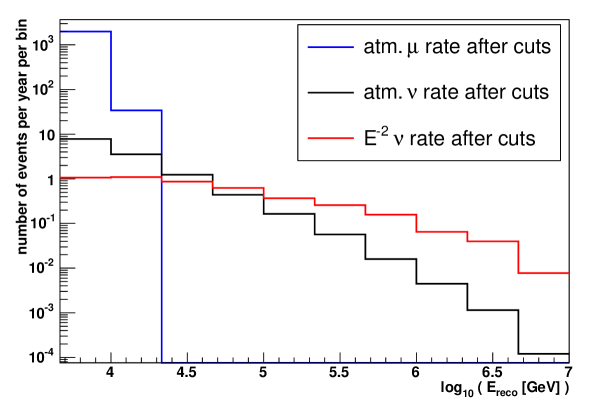
Figure 10.13: Rates for isotropic shower events: atmospheric muons (blue) and atmospheric (black) and cosmic (red) neutrinos versus the reconstructed energy.

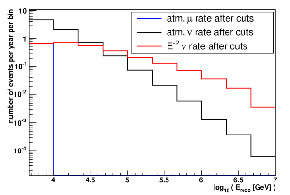
Figure 10.14: Rates for upgoing shower events: atmospheric muons (blue) and atmospheric (black) and cosmic (red) neutrinos versus the reconstructed energy.

From the background rates shown in Figure 10.13, one can deduce an upper limit of the experiment for a diffuse flux, as has been described in Section 3.3.2. Above 20 TeV, no atmospheric muons are present in the sample. The cosmic neutrino rate exceeds the atmospheric neutrino rate above 50 TeV. The atmospheric neutrino rate above this energy is 0.70/year. The number of events to reject the background-only hypothesis at a 90% confidence level for the expected background rate is [Fel98] $N=3.77$. A parameterisation of the total effective area for shower events as a function of the neutrino energy, needed for the calculation of the flux limit, is shown in Figure 10.15. Assuming a cosmic neutrino flux proportional to $E^{-2}$, one receives, according to equation 3.16 and the quoted number of events, a flux limit of

$$E_{\nu}^{2}{\Phi_{90\%}}=1.7\times 10^{-7}\,\textrm{GeV cm}^{-2}\,\textrm{s}^{-1}\,\textrm{sr}^{-1}$$ (10.3)

after the cuts mentioned above.

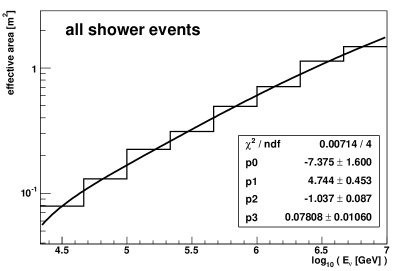
Figure 10.15: Total effective area for isotropic shower events, and fit used for flux limit estimations.

The result from equation (10.3) can be compared to the flux limit to shower events of the AMANDA detector [AMA04a], where the expected background above $\sim 50$ TeV is $0.90^{+0.69}_{-0.43}$ atmospheric muon events, and $0.06^{+0.09}_{-0.04}$ atmospheric neutrinos, assuming a different model for the conventional flux [Lip93] and disregarding the prompt neutrino flux because of its large uncertainties [Kow04]. In the analysed data taken in 2000, one event remains after the cuts. The authors derive from this an upper limit for the flux of neutrinos of all flavours in AMANDA of

$$E_{\nu}^{2}{\Phi_{90\%}}^{\textrm{AMANDA}}=8.6\times 10^{-7}\,\textrm{GeV cm}^{-2}\,\textrm{s}^{-1}\,\textrm{sr}^{-1},$$ (10.4)

at 90% confidence level, assuming a mean background of 0.96 events. This limit is approximately a factor of 5 higher than the result retrieved in this study, which may point to an underestimation of the atmospheric muon flux; however, also the effective areas presented in this study are larger by about a factor of 2 than those shown in [AMA04a].
The flux limit derived here is shown in comparison to other measured and expected rates in Figure 10.16. It is around a factor 2.2 above the flux limit for charged $\nu_{\mu}$ events expected in ANTARES for the same measurement period [Zor04] (grey line marked “ANTARES $\mu$ 1 year”). See Figure 4.15 in Section 4.6 for an explanation of the experimental limits, and Figure 3.10 in Section 3.3.4 for a description of the theoretical predictions.

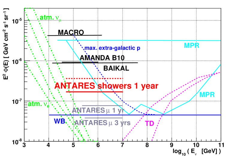
Figure 10.16: Flux limits for isotropic (drawn red line) and upgoing (dashed red line) shower events in ANTARES, as determined in this study, in comparison to results for other event types or experiments. See Figure 4.15 in Section 4.6 for a description of the other limits.

As the angular resolution of the shower reconstruction is about $2^{\circ}$ above some 10 TeV after the cuts, only upgoing events can be considered as well. Both the events from sample B and the $\nu_{e}$ CC events were produced with isotropic neutrino distributions, and therefore, the original number of upgoing neutrinos was considered to be half of the total number of events produced. The effective areas for upgoing events can then be determined, and from this and from the expected background rates, the expected flux limit for upgoing events can be calculated. The effective areas from which the upgoing flux limit was retrieved are shown in Figure 10.17, for NC events (left) and $\nu_{e}$ CC events (right), in comparison to the effective areas of isotropic events. While the effective area for neutrino energies below $\sim 100$ TeV is slightly larger for upgoing events because of their better reconstructibility, above this value, the effective area flattens because of the opaqueness of the Earth (see Section 3.2.2). Consequently, also the flux limit for the highest energy bins, as well as the overall flux limit, will be worse for the upgoing events than for the events distributed isotropically.

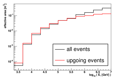
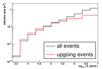
Figure 10.17: Effective areas for NC events (left) and $\nu_{e}$ CC events (right), for isotropic events (black lines) and for upgoing events (red lines).

As for the isotropic events, the energy-independent flux limit of the upgoing events was calculated by parameterising the effective area in the relevant energy region. The parameterisation function of the total effective area for upgoing shower events as a function of the neutrino energy, for energies above 5 TeV, is shown in Figure 10.18.

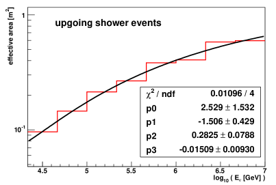
Figure 10.18: Total effective area for upgoing shower events, and fit used for flux limit estimations.

From Figure 10.14, the expected atmospheric neutrino background above 50 TeV is 0.35 events per year, and the atmospheric muon background above 50 TeV is negligible, so that the case of zero measurement can be considered, which yields a maximum number of 2.12 events for the expected background rate at 90% confidence level [Fel98]. For this case, one receives an energy-independent flux limit of

$$E_{\nu}^{2}{\Phi_{90\%}}^{up}=3.6\times 10^{-7}\,\textrm{GeV cm}^{-2}\,\textrm{s}^{-1}\,\textrm{sr}^{-1},$$ (10.5)

a slightly larger value than for the isotropic neutrino flux, and around a factor 4.7 larger than the expected ANTARES flux limit for $\nu_{\mu}$ CC events. The flux limit for upgoing events is shown in Figure 10.16 as dashed lines.

Conclusion

The feasibility of reconstructing neutrino-induced showers with a precision of down to $2^{\circ}$ in angular resolution has been demonstrated. A number of cuts had to be applied to sufficiently suppress the atmospheric muon background; the flux expected from this background lies now below the neutrino flux, for energies above 20 TeV for isotropic, and above 5 TeV for upgoing events, so that it is possible to study the diffuse neutrino flux above these energies. Sensitivities both for isotropic and upgoing shower events have been calculated, and they are found to be around a factor 2–5 above the flux limit for charged $\nu_{\mu}$ events expected in ANTARES for the same measurement period [Zor04] (grey line marked “$\mu$ one year” in Figure 10.16). This ratio agrees well with the rough flux limit estimation given in Section 3.3.3, where a deterioration of a factor 5 was predicted. It can therefore be concluded that the shower reconstruction strategy adds an important, independent contribution to the measurable neutrino flux in ANTARES.

Chapter 11 Summary and Outlook

This thesis is devoted to the reconstruction of shower-type events with the ANTARES detector, a neutrino telescope that is currently being installed in a depth of 2400 m in the Mediterranean Sea. The main objective of ANTARES is the detection of high-energy cosmic neutrinos that are presumably produced in astrophysical objects like Supernova Remnants, Active Galactic Nuclei or Gamma Ray Bursts. The detection of these neutrinos will permit a new insight into the physics of these objects. Neutrinos are detected by measuring the Cherenkov light signal that is caused by the charged secondary particles of a neutrino interaction with matter, in this case, the water of the deep sea. The amplitudes and timings of the light signals are measured in photomultiplier tubes inside Optical Modules, which are installed covering a volume of $\sim 0.03$ km³. From the signals, the direction and energy of the neutrinos are to be reconstructed.
Depending on the type of neutrino interactions, different secondaries can be generated, and different strategies must be used to reconstruct them. This thesis deals with the reconstruction of neutrino-induced showers, both hadronic and electromagnetic. Showers are present in all neutrino interactions, and there are two types of reactions for which they are the only detectable objects: Neutral current (NC) interactions and charged current (CC) electron neutrino interactions. It has been shown in this thesis that both event types can be reconstructed using the same strategy.
Neutrino telescopes are usually optimised on the reconstruction of muons from CC muon neutrino interactions. In these events, a muon and a hadronic shower are produced in the interaction of the neutrino with the ambient matter. For the considered energies above a few 100 GeV, the muon has a path length of 1 km or more and its direction can be reconstructed to a precision of a few tenth of a degree. Showers, on the other hand, occur on a relatively small scale with respect to the spacing of the Optical Modules in the detector – the typical length of a shower is 10 m, while the distance between the Optical Modules of the detector is 14.5 m in vertical, and 60 to 75 m in horizontal direction. Therefore, the directional characteristics of a shower cannot be resolved well in the ANTARES detector, so that a sub-degree angular resolution, as reached for muons, is not achievable for showers. On the other hand, since the showers have considerably small dimensions, almost the entire amount of light produced in the shower can be detected, which makes the reconstruction of the shower energy much less problematic.
A strategy to reconstruct the shower direction together with the shower energy has been developed in the context of this thesis. The first reconstruction step is the determination of the position of the shower maximum, which is calculated assuming an isotropic emission of light. Direction and energy are then determined using a pattern matching algorithm: The signal amplitudes that have been measured in the Optical Modules of the detector are compared to those that are calculated assuming specific values for shower direction and energy, taking into account the angular efficiency of the photomultipliers, the absorption of the photons in water and the energy dependent angular distribution of the photons with respect to the shower axis. Direction and energy are then determined using log-likelihood optimisation.
The reconstruction of the shower events yields an overall median of the directional error of the shower about $10^{\circ}$, both for NC and $\nu_{e}$ CC events, for reconstructed energies above 5 TeV. The width of the peak in the logarithmic shower energy resolution is $\sim 0.19$ which means that the shower energy can be determined to a factor of ${10^{0.19}\approx 1.5}$. Some additional quality cuts which proved to have a high combined efficiency and purity have been applied to the data samples. The combined efficiency of all cuts it at about 70%. After the cuts, the reconstruction of the shower energy improves to a factor of ${10^{0.16}\approx 1.4}$. The directional resolution improves to $3.5^{\circ}$, with values at $2^{\circ}$ for energies of about 100 TeV. Since the background dominates the neutrino signal below $\sim 50$ TeV (see below), the reconstruction algorithm is optimised to the energy region above this value.
When deducing the neutrino energy from the shower energy, it must be taken into account that for NC events, a part of the primary neutrino energy is carried away by the outgoing neutrino. This fraction could be determined statistically, but as NC events will not be distinguishable in the experimental data from $\nu_{e}$ CC (for which the shower energy is equivalent to the neutrino energy), it was preferred for this study to regard the reconstructed shower energy a priori as a lower limit for the primary neutrino energy.
The results presented here were obtained assuming the saturation of the photomultiplier electronics at 200 photo-electrons. However, the data taking mode which would enable this high saturation level is very bandwidth-consuming. It has been found that under the assumption of a saturation at 20 photo-electrons, which is the saturation level corresponding to the default data taking mode in ANTARES, the resulting resolution below 70 TeV is slightly better than for a higher saturation, because the large fluctuation effects that occur at these smaller energies are damped by the lower amplitude saturation. For higher energies, the lower saturation leads to a slight deterioration in the angular resolution, which becomes about $3^{\circ}$ larger than the resolution achieved for the saturation at 200 pe. The energy resolution shows very similar results for both saturation levels.
As the ANTARES detector is not built in a sterile surrounding, but in natural salt water, the Optical Modules are exposed to constant optical noise from ⁴⁰K decays and from bacteria bioluminescence. The background can be suppressed by applying filter conditions on the signals in the individual Optical Modules, concerning the causal connection of the signal with the signals in the other Optical Modules, and the size of the signal amplitude. The filter works most efficiently for events with shower energies above $\sim 10$ TeV.
A second type of background originates from high-energy particle interactions caused by atmospheric muons and atmospheric neutrinos.
Atmospheric muons are a dangerous background to neutrino-induced showers if they cannot be clearly identified as muons, either because they undergo strong bremsstrahlung losses from which an electromagnetic cascade is produced, or because they occur as multi-muon bundles. Over 99% of the atmospheric muon background are suppressed by some quality cuts; the background becomes negligible above 20 TeV.
Atmospheric neutrinos are an insuppressible background to cosmic neutrinos; the latter can only be identified by detecting an excess of events over the atmospheric neutrino spectrum.
Due to the background of atmospheric neutrinos, which dominates the signal of shower events from cosmic neutrinos below $\sim 50$ TeV, the detection of an isotropic, diffuse cosmic flux is only possible above this energy. The expected isotropic rate for atmospheric neutrinos above this energy was determined as 0.70/year. At a 90% confidence level and under the assumption of the detection of one background event, this yields an energy-independent upper limit on the cosmic neutrino flux of

$$E_{\nu}^{2}{\Phi_{90\%}}=1.7\times 10^{-7}\,\textrm{GeV cm}^{-2}\,\textrm{s}^{-1}\,\textrm{sr}^{-1}$$

for one year of data taking in ANTARES, assuming that the cosmic neutrino flux is proportional to $E^{-2}$. If only upgoing events are considered, the atmospheric muon background (consisting of downgoing events which have been misreconstructed as upgoing) above 5 TeV is negligible, and the atmospheric neutrino rate is 0.35/year. The corresponding upper limit on the cosmic neutrino flux for one year of data taking in ANTARES, assuming no event detection at all, becomes then

$$E_{\nu}^{2}{\Phi_{90\%}}^{up}=3.6\times 10^{-7}\,\textrm{GeV cm}^{-2}\,\textrm{s}^{-1}\,\textrm{sr}^{-1}.$$

These flux limits are about a factor 2–5 larger than those predicted for the CC muon neutrinos in ANTARES, due to the smaller effective area for shower events.
While all other reconstruction strategies for the ANTARES detector are intended for CC muon neutrino events, the strategy introduced here allows now to also reconstruct shower events. It therefore closes an important gap in the ANTARES event reconstruction, as now the reconstruction of all event topologies is possible, and the access to events which were unreconstructible until now is permitted. The detectable neutrino flux for the ANTARES detector has therefore been significantly increased.
The shower reconstruction could also lead to an important improvement in the reconstruction of the neutrino energy for $\nu_{\mu}$ CC events, if the event has taken place close enough to the instrumented volume for the hadronic shower to be detected as well. In this case, the muon and the hadronic shower could be reconstructed separately and the results could be combined afterwards.
In principle, the strategy introduced here is adaptable to other experiments as well; the parameterisations used have been tuned to the ANTARES detector, but could be tuned to other detectors as well. For experiments at sites with a significantly shorter scattering length, like IceCube, the strategy is probably not applicable, because the directional characteristics of the Cherenkov photons of the shower are deteriorated too strongly to permit a reconstruction.

Appendix A ANTARES Event Simulation Packages

In this appendix, the software chain for the production of ANTARES Monte Carlo (MC) events is described, as far as it was used for the presented study. The MC production is usually divided into four parts: The interaction of the neutrino, which is simulated with genhen, see Section A.1; the propagation of secondaries and the production of Cherenkov light, for which geasim is used in the case of non-muonic events, see Section A.2; the selection of physics hit from noise hits, for which a software filter is used, see Section A.3; and finally the event reconstruction, which is done with reco, see Section A.4.
The chapter closes with a description of the different data samples used for this study in Section A.5.
A more detailed summary of the ANTARES simulation tools can be found in [Bru03]. As the main part of this work, the ShowerFitter, a reconstruction package for showers, was developed within the reco frame. The physical and mathematical background of this shower reconstruction is described separately in Chapter 8.

A.1 Monte Carlo Event Generation: genhen

Genhen [Bai00, Kuz04] is an event generator for ANTARES events written in Fortran. From version v6 upwards, the generation of events from all neutrino flavours is supported. To generate NC or $\nu_{e}$ CC events using genhen, the user defines a cylindrical object called can within which the events are generated. Depending on the event type, the can extends up to a few hundred metres beyond the instrumented volume, but for the generation of shower events, which have a relatively short range, an extension of a few absorption lengths is sufficient. If a $\nu_{\mu}$ CC event is generated, the shower that accompanies the $\mu$ is only written into the genhen output if it occurs close enough to the detector to be measured; else, only the single muon is displayed.
The neutrino interactions are simulated using the LEPTO [Ing97] package for the deep inelastic scattering and the RSQ [Bar87] package for resonant and quasi-elastic events. The CTEQ parton distribution functions [Lai95] are used as default; the most recent version which can be used is CTEQ6D. The hadronisation is done using PYTHIA/JETSET [Sjo94]. The neutrino energy range in genhen is valid from the lower energy threshold of the detector, a few dozen GeV, up to 1 EeV. However, due to uncertainties in the structure functions, the total uncertainty in the neutrino cross section exceeds 10% at 100 PeV; and for neutrino energies above 1 PeV, also the results from PYTHIA and JETSET, which are originally intended for particle accelerator physics, and therefore tuned for lower energies, might be wrong.
The output of genhen consists of the primary neutrino, its kinetic properties and the position of the interaction vertex, plus the position, direction and energy of the long-lived secondaries that were produced by the interaction. For secondaries with a lifetime $\lesssim 10^{-11}$ s, the respective decay products are displayed in the output instead.
The program also calculates and displays event weights which take into account the absorption probability of neutrinos on their passage through the Earth, and gives event rates for an assumed neutrino flux.

A.2 Particle Tracking and Light Generation: geasim

In the ANTARES software chain, the tracking of particles other than muons is done with the geasim package [Gea00] which is based on GEANT 3.21 [Gea93]. All relevant physics processes that can occur during the passage of particles through a medium are taken into account. At each tracking step of each particle, a Cherenkov cone is produced; if an OM lies within the rays of light from the cone, a hit is produced, whose amplitude is calculated according to the photon density on the cone, using Poissonian statistics. The the characteristics of the PMTs, like quantum efficiency, angular efficiency or the transmission coefficient of the glass sphere are taken into account as well, as is the wavelength-dependent attenuation of light in water (see Section 4.4). However, scattering effects are not simulated; the number of photons is only damped according to the attenuation length.
The radial size of the shower is neglected in geasim as it is only a few cm. Monte Carlo studies have shown that the angular distribution of the Cherenkov light with respect to the shower axis is not energy-dependent for electromagnetic showers (see Section 5.2). Therefore, this distribution has been parameterised to save CPU time. For hadronic showers, however, the distribution is energy-dependent; it is subject to large fluctuations and therefore no parameterisation is done. It is thus necessary to track every single particle in the shower down to the Cherenkov level. This is very time-consuming, and the CPU time rises exponentially with energy, as can be seen in Figure A.1, where the average CPU time for the processing of one event is shown. The average CPU time was determined by processing 10 mono-energetic events for each decade of energy, so fluctuations are possible, but the trend is clearly visible.

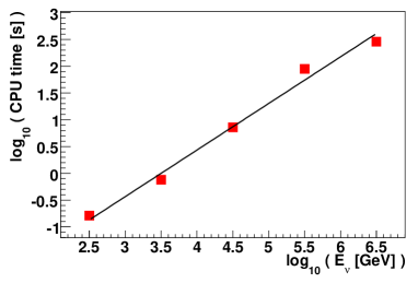
Figure A.1: CPU usage of one event in geasim as a function of the neutrino energy.

This high consumption of time makes the production of events above $\sim 10$ PeV a tedious business. There are also some known errors in the cross sections from GEANT 3.21. The authors of geasim therefore do not recommend the usage above 100 TeV, although events have been produced within this work up to energies of 100 PeV without displaying any obvious flaws other than technical ones.
After the event processing, the output of geasim is added to the event file generated by genhen. The geasim output consists of a list of all OMs which have been hit, the amplitude of the hits, their timing, particle of origin and track of origin. The hit digitisation in the PMTs is simulated by producing the so called raw hits from the hits. For this, data taking characteristics (see Section 4.3.1) like the ARS integration time of 25 ns, the number of ARSs and the dead times are taken into account. The timing information can be smeared by a Gaussian (as was done for the data used in this study) or a Laplace distribution. The raw hits do not contain any MC information any more, as they are intended to be in the same format as measured signal hits.
In geasim, it is also possible to add optical background. To do this, the user defines the required background frequency; geasim will then add random single photon hits to the events according to that frequency.

A.3 Hit Selection: Software Filter

For real data, a software trigger will be used to decide whether the detector has measured a physics event or only noise. This trigger collects hits that are causally connected and/or have a sufficiently large amplitude; when the trigger conditions are fulfilled, a physics event is built. The selection criteria can also be used as a filter to eliminate noise hits in a MC event sample, as has been described in the chapter on different sources of background, in Section 6.4. In this case, only the hits passing the filter conditions will be used for further analysis. If an event, after the filter has been applied to it, does not contain a sufficient number of hits for reconstruction, it will be discarded. In the final version of the event simulation, the filter conditions will be applied to the events in a stage between the hit generation and the reconstruction. For this study, the filter conditions were part of the reconstruction code that is described in the next section.

A.4 Event Reconstruction: reco

Reco is the ANTARES reconstruction package within which different reconstruction algorithms, the so called strategies, can be placed and run. The software in its current form was re-written from the previously existing code in 1999 by [Cas99a]. Information on the code structure and a collection of documentation can be found on the reco home-page [Sto05]. There exists also a handbook on different reco strategies [Rom01] which describes some of the algorithms and their implementation in the code.
Almost all reconstruction algorithms which have been developed for the ANTARES detector until now are intended for the reconstruction of $\nu_{\mu}$ CC events. There is one strategy called BrightPointFitter which reconstructs the position of a point source of light by calculating the centre-of-gravity of all hits in an event. The same algorithm is also used for the reconstruction of the vertex in a shower event, as described in Section 7.1. A reconstruction strategy for showers has been developed in 2000 by [Ber00] but it was never integrated into the official ANTARES reconstruction code.

General Remark on the Data Format

At the writing of this thesis, the standard format of the event files was in ASCII code. However, work is going on to change this into the ROOT [Bru96] format, and this process will probably be completed within the first half of 2006. The new data format forsees a stricter separation between physics characteristics of an event and characteristics that are caused by the detector properties. For example, the conversion from hits to raw hits, and the addition of optical background, will not be done any more within the simulation of the particle tracking and light production, but in a separate program devoted for digitisation and triggering.

A.5 The Monte Carlo Data Samples

This section describes the different MC data samples that were used for this thesis. Both NC events and $\nu_{e}$ CC events have been studied. Atmospheric muon background was studied as well, using events which were produced within the ANTARES collaboration. This section summarises the characteristics of the used samples: the neutrino energy range and spectrum, the angular distribution of the neutrino, the optical background that was added and the remaining event numbers after the different steps of the reconstruction.

A.5.1 The NC Events

Event Sample A

The Monte Carlo distributions and some of the results shown in this note are based on a $\nu_{e}$ NC data sample of 4776 events between $10^{2}$ and $10^{8}$ GeV, called event sample A within this thesis. The neutrino energy spectrum of this production is $E^{-1}$ and the angular distribution is isotropic over $4\pi$. The sample is available without optical background and with different rates of optical background, between 60 kHz and 140 kHz, as well. Note that 60 kHz is the default background rate used with this sample, as long as no other background rate is implicitly mentioned in the text. The can inside which the events were produced was of about the size of the instrumented volume of the ANTARES detector, thus the events can be considered to be contained events.

Event Sample B

Because the statistics of the above-mentioned event sample A are rather limited, $\nu_{\mu}$ NC events that were part of a $5\times 10^{5}$ events mass production of shower-type events were used where larger statistics were required. These events are denoted as event sample B. The events were produced with a neutrino energy between $10^{2}$ and $10^{7}$ GeV, an energy spectrum of $E^{-1}$ and inside a generation volume that exceeds the instrumented volume by one absorption length ($\sim 55$ m). The primary neutrinos were distributed isotropically in the whole $4\pi$ solid angle. An optical background of 60 kHz was added to these events as well. The numbers of events in event sample B, after the different stages of event production as described in the first four sections of this chapter, are given in Table A.1. Figure A.2 (top) shows these numbers in relation to the number of originally generated events, again for the different energy bins. As expected, the percentage of events that survive all production stages increases with increasing energy, because the number of produced photons is proportional to the shower energy, and the filter and reconstruction stages become more efficient for larger numbers of hits. It should also be noted that the filter efficiency is worse than for the events shown in Figure 6.6 in Section 6.4.2, because the events shown there are contained events.

neutrino energy [GeV]	generated (Section A.1)	producing hits (Section A.2)	filtered (Section A.3)	reconstructed (Section A.4)
$10^{2}-10^{3}$	99633	67266 (67.5%)	1935 (1.94%)	1747 (1.75%)
$10^{3}-10^{4}$	22623	20000 (88.4%)	5541 (24.5%)	5142 (22.7%)
$10^{4}-10^{5}$	10318	10000 (96.9%)	5939 (57.6%)	5486 (53.2%)
$10^{5}-10^{6}$	5040	5000 (99.2%)	4085 (81.1%)	3739 (74.2%)
$10^{6}-10^{7}$	2465	2457 (99.7%)	2288 (92.8%)	2115 (85.8%)
total events	140079	104723 (74.8%)	19788 (14.1%)	18229 (13.0%)

Table A.1: Numbers of events in event sample B, after the different production stages. The percentages given refer to the original number of events (first column).

The sample also contains event weights for the atmospheric neutrino flux, according to the Bartol model [Agr96], which were calculated during the simulation (see Section A.1). Beside the conventional neutrino flux, prompt neutrinos were taken into account as well, according to the studies of [Nau01] and using the recombination quark-parton model (RQPM) [Bug98].

A.5.2 The $\nu_{e}$ CC Events

The $\nu_{e}$ CC events which were used for this study were produced within the same mass production and with the same simulation parameters as event sample B of the NC events (see above). The energy of the primary neutrino lies between $10^{2}$ and $10^{7}$ GeV. The energy spectrum used for the production is $E^{-1}$, and the events were produced inside a generation volume that exceeds the instrumented volume by one absorption length ($\sim 55$ m). The primary neutrino was distributed isotropically in the whole $4\pi$ solid angle. A optical background of 60 kHz was added. As for event sample B, event weights for the atmospheric neutrino flux according to the Bartol model [Agr96] and including prompt neutrinos [Nau01] were added as information to each event.
The event sample was chosen from the mass production to be originally of about the same size as event sample B of the NC events; as all energy of the primary neutrino goes into showers for this event type, the showers in these events are actually more energetic than the those in the NC events from the same mass production, and thus, a larger number of events than for the NC events remains in the sample after the different production stages. The numbers of events for the different energy bins and the different stages of production are given in Table A.2. Figure A.2 (bottom) shows these numbers in relation to the number of originally generated events over the shower energy of the respective bin. The percentage of events that survive all production stages rises with increasing energy; however, the fraction of actually reconstructed events is lower in the highest energy bin than than in the second-highest one, an evidence for the fact that for some of the events, saturation effects in the OMs keep the reconstruction from converging.

neutrino energy [GeV]	generated (Section A.1)	producing hits (Section A.2)	filtered (Section A.3)	reconstructed (Section A.4)
$10^{2}-10^{3}$	100270	85068 (84.8%)	8326 (8.30%)	7610 (7.59%)
$10^{3}-10^{4}$	20506	20000 (97.5%)	9774 (47.7%)	9056 (44.2%)
$10^{4}-10^{5}$	10007	10000 (99.9%)	8224 (82.2%)	7514 (75.1%)
$10^{5}-10^{6}$	5000	5000 (100%)	4926 (98.5%)	4483 (89.7%)
$10^{6}-10^{7}$	2757	2757 (100%)	2757 (100%)	2499 (90.6%)
total events	138540	122825 (88.7%)	34007 (24.5%)	31162 (22.5%)

Table A.2: Numbers of events in the $\nu_{e}$ CC event sample, after generation, hit production with geasim, the filter conditions, and the reconstruction. The percentages given refer to the original number of events (first column).

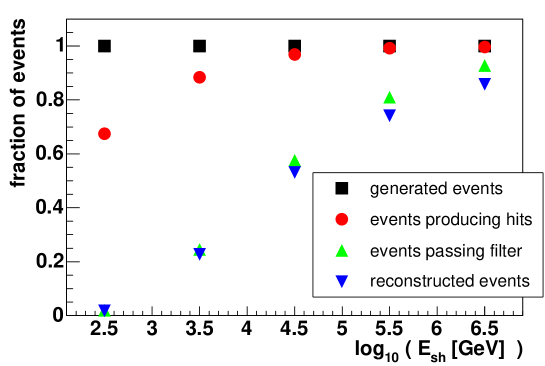
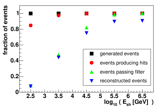
Figure A.2: Number of NC events from sample B (top) and number of $\nu_{e}$ CC events (bottom) after the different stages of production as listed in tables A.1 and A.2, over the shower energy. The event numbers have been normalised to the respective numbers of generated events.

A.5.3 The Atmospheric Muon Background

For the studies on the suppression of the atmospheric muon background that are discussed in Section 9.1, a sample of atmospheric muons produced in 2005 at Bologna for the ANTARES collaboration was used. The whole data sample is described in more detail in [Mar05b]. It contains events with protons, helium, nitrogen, magnesium or iron as primaries interacting in the atmosphere, produced within different energy and zenith angle ranges. For the results shown here, only the proton events were used.
For the higher energies, due to the high amount of CPU usage, only about 10% of the whole production were used.
Table A.3 shows the numbers of events in the different energy and angular bins for the used data sample.

zenith angle	$0^{\circ}-60^{\circ}$			$60^{\circ}-85^{\circ}$
energy [TeV/nucleon]	1-10	10-100	100-105	1-10	10-100	100-105
primary protons	$10^{8}$	$10^{7}$	$10^{7}$	$10^{8}$	$10^{7}$	$10^{7}$
approx. equiv. lifetime	$\sim 1$ h	$\sim 2.6$ h	$\sim 6$ days	$\sim 1$ h	$\sim 2.6$ h	$\sim 6$ days

Table A.3: Numbers of events in the different energy and angular bins of the atmospheric muon event sample.

The primary spectrum used was $E^{-2}$; the air showers from the primaries were produced using the CORSIKA package [Hec98], version 6.203. After the production of secondaries in CORSIKA, the secondary muons were propagated to the detector with MUSIC [Ant97], and the detector response was simulated using km3 [Nav99]. A optical background of 60 kHz was also added to the data sample.

Appendix B Technical Details of the ShowerFitter Package

B.1 Parameters Used for the Reconstruction

Table B.1 lists the fixed parameters that were used in the reconstruction, and their values.

Parameter	Value	Source/comment
refraction index $n$	1.3499	[Cas99b]
photon wavelength $\lambda$	475 nm	minimal absorption
absorption length $\tau$	54.9451 m	for $\lambda=475$ nm, [Cas99b]
PM saturation	200 pe / 20 pe	WF mode / SPE mode
minimum pe threshold	0.3 pe
filter parameters (see Section 6.4.1):
causality time window $\delta t$	100 ns	condition 1
minimum amplitude $A_{min}$	3 pe	condition 2
coincidence time window	20 ns	condition 2
number of coincidences on one string	2	condition 3
minimum amplitude $A_{min,2}$	1.5 pe	condition 3
minimum number of hit strings	3	filter condition

Table B.1: List of the values of environmental and data acquisition parameters used in the ShowerFitter.

B.2 Schematic Description of the Fit

A schematic process chart of the whole ShowerFitter strategy, its parameters and the references to the descriptions of the respective steps in the chapters of this work, is provided in Figure B.1.

Figure B.1: Reconstruction Scheme of the ShowerFitter. The parameters that are determined in the respective reconstruction step are listed in the boxes on the right of the figure.

Appendix C Error Calculations

C.1 Calculation of the Errors on Efficiency and Purity

Efficiency and purity are both functions of the form $f(n,n_{1})=\frac{n_{1}}{n}$. As $n_{1}$ is a subsample of $n$, and therefore not independent from it, the error propagation rules cannot be used directly. Instead, one defines $n\equiv n_{1}+n_{2}$. The function $f$ becomes then $f(n_{1},n_{2})=\frac{n_{1}}{n_{1}+n_{2}}$ with the two independent variables $n_{1}$ and $n_{2}$. The error on $f,\,\sigma_{f}$, can then be calculated following the Gaussian error propagation rules:

$$\sigma_{f} =\sqrt{\left(\frac{df}{dn_{1}}\right)^{2}\sigma_{n_{1}}^{2}+\left(\frac{df}{dn_{2}}\right)^{2}\sigma_{n_{2}}^{2}}$$ (C.1)

$$=\sqrt{\left(\frac{n_{2}}{(n_{1}+n_{2})^{2}}\right)^{2}\cdot n_{1}+\left(\frac{-n_{1}}{(n_{1}+n_{2})^{2}}\right)^{2}\cdot n_{2}}$$

$$=\sqrt{\frac{(n_{2})^{2}n_{1}}{(n_{1}+n_{2})^{4}}+\frac{(n_{1})^{2}n_{2}}{(n_{1}+n_{2})^{4}}}$$

$$=\sqrt{\frac{n_{1}n_{2}(n_{2}+n_{1})}{n^{4}}}$$

$$=\frac{\sqrt{n_{1}(n-n_{1})n}}{n^{2}}.$$ (C.2)

If the subsample $n_{1}$ is equal to $n$ (and therefore, $n_{2}=0$), one can no longer assume that the statistical error of the variable $n_{2}$ is $\sqrt{n_{2}}$ (this would always result in $\sigma_{f}=0$, no matter how large or small $n$ is). Instead, one has to take into account Poissonian statistics: For a $1\sigma$ error, (100 - 68 = 32)% of the events lie outside the $1\sigma$ area. For the case of $n_{1}=n$, only the error in one direction has to be considered; the other one is really zero. Therefore, one has to define the Poisson distribution such that 32% / 2 = 16% of the events lie outside of the curve. 84% should thus lie inside. The normalised Poisson distribution thus should solve to

$$\int_{0}^{t}P(x,0)=\int_{0}^{t}\frac{x^{0}e^{-x}}{0!}=\int_{0}^{t}e^{-x}=-e^{-t}+e^{0}=1-e^{-t}=0.84$$ (C.3)

$$\leadsto t=-\ln 0.16\approx 1.83=\sigma_{n_{2}}.$$ (C.4)

Equation (C.1) therefore becomes

$$\sigma_{f}=\sqrt{\left(\frac{-n}{n^{2}}\right)^{2}\sigma_{n_{2}}^{2}}=\frac{\sigma_{n_{2}}}{n}=1.83/n.$$ (C.5)

C.2 Standard Error on the Median

For the calculation of the standard error on the median, the derivation from the book of Kendall and Stuart [Ken63, pp.236-237] was used:
A frequency distribution can be described by quantiles, i.e. the $(m-1)$ values which divide a frequency distribution into $m$ equal parts (i.e. with an equal number of entries). The most common quantile is the median, which divides a frequency distribution into 2 equal parts.
If a sample of $n$ values distributed according to a frequency distribution $f(x)$ is considered, with a fraction of $pn$ values below and a fraction of $qn$ values above the quantile $x_{1}$, it can be shown that the variance $V(x_{1})$ is given by

$$V(x_{1})=\frac{pq}{nf(x_{1})^{2}}.$$ (C.6)

In the case of the median, $p=q=\frac{1}{2}$, and therefore $V(x_{m})=\frac{1}{4nf(x_{m})^{2}}$, where $x_{m}$ is the value of the median. Assuming that the distribution is normal with a variance $\sigma^{2}$, the standard error on the median $\sigma_{m}$ becomes

$$\sigma_{m}=\sigma\cdot\sqrt{V(x_{m})}=\sigma\cdot\frac{1}{2\sqrt{n}f(x_{m})}.$$ (C.7)

As $x_{m}=0$ for the normal distribution, ${f(x_{m})=\frac{1}{\sqrt{2\pi}}\exp\{-\frac{1}{2}x_{m}^{2}\}=\frac{1}{\sqrt{2\pi}}\approx 0.399}$. The standard error on the median becomes therefore

$$\sigma_{m}=1.253\cdot\frac{\sigma}{\sqrt{n}}.$$ (C.8)

Danksagung

Eine Vielzahl von Menschen hat zum Gelingen dieser Arbeit beigetragen, und ich bin allen zu großem Dank verpflichtet.
Zuallererst danke ich meinem Betreuer, Prof. Dr. U. Katz, dafür, dass er es mir ermöglichte, meine Arbeit zu einem so interessanten Thema zu schreiben, und mir während meiner Zeit als Doktorandin unermüdlich mit Rat und Tat zur Seite stand.
Prof. Dr. E. Steffens hat sich freundlicherweise bereit erklärt, das Zweigutachten zu meiner Arbeit zu schreiben, wofür ihm herzlicher Dank gebührt.
I would like to thank the ANTARES collaboration for the friendly and fruitful atmosphere that I have experienced while being a member of the collaboration. I especially thank Jürgen Brunner for his prompt answers to my emails and his help in all technical and software questions.
Ich danke allen Kollegen der Erlanger ANTARES-Gruppe für die angehme Arbeitsatmosphäre und die gute Zusammenarbeit, und auch den Nicht-ANTARESianern von Abteilung 1 und 4 für die gute Gesamtstimmung im Institut, ob beim gemeinsamen Gang zur Mensa (die dort gereichte Kost wäre ohne Gesellschaft jedenfalls nicht auf Dauer auszuhalten!), bei der Kaffeerunde oder auf diversen Festivitäten.
Besonderer Dank gebührt Alexander Kappes, der nicht nur die Arbeit gründlich Korrektur gelesen hat, sondern sich auch immer die Zeit genommen hat, physikalische Fragen zu diskutieren und technische Probleme zu lösen, sowie Felix Fehr und Kay Graf für das sorgfältige Korrekturlesen meiner Arbeit. Bei Kay Graf bedanke ich mich außerdem für den seelischen und moralischen Beistand insbesondere während der arbeitsreichen Zeit des Zusammenschreibens ♡.

LEBENSLAUF

Persönliches
Name: Bettina Diane Hartmann Adresse: Gerhart-Hauptmann-Straße 11 91058 Erlangen Telefon: 09131 – 16 06 79 E-Mail: hartmann@physik.uni-erlangen.de Geburtsdatum: 14. Februar 1977 Geburtsort: Stuttgart

beruflicher Werdegang
Bildung 1987 – 1996 Hölderlingymnasium Stuttgart August – Oktober 1993 Bexley Highschool, Columbus, Ohio, USA Oktober 1996 – Juni 2002 Universität Karlsruhe (TH): Physik (Diplom) September 2002 – März 2006 Universität Erlangen–Nürnberg: Promotion Prüfungen Juni 1996 Abitur, Note: 1,3 Oktober 1998 Vordiplom, Note: 2,5 Juni 2002 Diplom, Note: 1,4 Juni 2006 Promotionsprüfung Diplomarbeit: Mai 2001 – Juni 2002 am Institut für Experimentelle Kernphysik Karlsruhe bei Prof. Dr. W. de Boer Thema: Suche nach einem leichten Higgsboson im $WH$-Kanal bei CDF mit neuronalen Netzen Doktorarbeit: seit September 2002 am Physikalischen Institut I der Universität Erlangen-Nürnberg bei Prof. Dr. U. Katz Praktika September & Oktober 1999 Praktikum am Institut für angewandte Physik an der Technischen Universität Kaunas, Litauen Juli & August 2000 Sommerstudentin am Forschungszentrum CERN (Genf, Schweiz) Oktober 2000 Wissenschaftliche Ausstellungsbetreuerin am Deutschen Elektronen-Synchrotron DESY, Hamburg

References

- [AGA01] The AGASA Collaboration, M. Chikawa et al., “Cosmic Ray Energy Spectrum above eV Observed with AGASA”, Proc. 27th ICRC, Hamburg, Germany (2001) 333
- [AGA02] The AGASA Collaboration, M. Chikawa et al., “Upper Limit on Gamma-Ray Flux above eV Estimated by the Akeno Giant Air Shower Array Experiment”, Astrophys. J. 571 (2002) L117
- [Agr96] V. Agrawal et al., “Atmospheric neutrino flux above 1 GeV”, Phys. Rev. D 53 (1996) 1314
- [ALE05] The ALEPH, DELPHI, L3, OPAL, SLD Collaborations, the LEP Electroweak Working Group, the SLD Electroweak and Heavy Flavour Groups, “Precision Electroweak Measurements on the Z Resonance”, to be published in Phys. Rep., hep-ex/0509008 (2005)
- [Ale88] E. N. Alexeyev et al., “Detection of the Neutrino Signal from SN 1987A in the LMC Using the INR Baksan Underground Scintillation Telescope”, Phys. Lett. B 205 (1988) 209
- [AMA00] The AMANDA Collaboration, E. Andrés et al., “The AMANDA Neutrino Telescope: Principle of Operation and First Results”, Astropart. Phys. 13 (2000) 1
- [AMA04a] The AMANDA Collaboration, M. Ackermann et al., “Search for Neutrino-Induced Cascades with AMANDA”, Astropart. Phys. 22 (2004) 127
- [AMA04b] The AMANDA Collaboration, M. Ackermann et al., “Search for Extraterrestrial Point Sources of Neutrinos with AMANDA-II Using Data Collected in 2000-2002”, submitted to Phys. Rev. Letters Rapid Communications, astro-ph/0412347 (2004)
- [ANT99] The ANTARES Collaboration, E. Aslanides et al., “A Deep Sea Telescope for High Energy Neutrinos”, astro-ph/9907432 (1999), http://antares.in2p3.fr/
- [ANT01] The ANTARES Collaboration, L. Thompson et al., “Recent results from the ANTARES deep-sea neutrino telescope”, Nucl. Phys. B Proc. Suppl. 91 (2001) 431
- [ANT02] The ANTARES Collaboration, P. Amram et al., “The ANTARES Optical Module”, Nucl. Instr. Meth. A 484 (2002) 369
- [ANT05a] The ANTARES Collaboration, J. A. Aguilar et al., “Transmission of light in deep sea water at the site of the ANTARES neutrino telescope”, Astropart. Phys. 23 (2005) 131
-
[ANT05b]
ANTARES status and news web site: “MILOM : a new major step”,
http://antares.in2p3.fr/News/MilOM/doc/index.html - [ANT05c] The ANTARES Collaboration, E. Falchini et al., “Status report on the ANTARES high energy neutrino detector”, Proc. 29th ICRC, Pune, India 00 (2005) 101
- [ANT05d] The ANTARES Collaboration, J. A. Aguilar et al., “Study of Large Hemispherical Photomultiplier Tubes for the ANTARES Neutrino Telescope”, Nucl. Instr. Meth. A 555 (2005) 132
- [Ant97] P. Antonioli et al., “A Three-Dimensional Code for Muon Propagation Through the Rock: MUSIC”, Astropart. Phys. 7 (1997) 357
- [Ath05] H. Athar, C. S. Kim and J. Lee, “The intrinsic and oscillated astrophysical neutrino flavor ratios”, hep-ph/0505017 (2005)
-
[Aug01]
The Pierre Auger Collaboration, J.W. Cronin et al.,
“Survey of the Pierre Auger
Observatory”, Proc. 27th ICRC, Hamburg, Germany (2001) 699,
http://www.auger.org/index.html - [Ave02] M. Ave et al., “Constraints on the ultrahigh-energy photon flux using inclined showers from the Haverah Park array”, Phys. Rev. D 65 (2002) 063007
- [Axf77] W. I. Axford, F. Leer and G. Skadron, Proc. 15th ICRC, Plovdiv, Bulgaria 11 (1977) 132
- [Bah99] J. Bahcall and E. Waxman, “High Energy Neutrinos from Astrophysical Sources: An Upper Bound”, Phys. Rev. D 59 (1999) 023002
- [Bah00] J. Bahcall, “How the Sun Shines”, published online at the site of the Nobel e-Museum: http://nobelprize.org/physics/articles/ and as astro-ph/0009259 (2000)
- [Bah01] J. Bahcall and E. Waxman, “High Energy Astrophysical Neutrinos: The Upper Bound is Robust”, Phys. Rev. D 64 (2001) 023002
- [Bah04] J. Bahcall, “Solving the Mystery of the Missing Neutrinos”, published online at the site of the Nobel e-Museum: http://nobelprize.org/physics/articles/ (2004)
- [BAI97] The BAIKAL Collaboration, I. A. Belolaptikov et al., “The BAIKAL Underwater Neutrino Telescope: Design, Performance and First Results”, Astropart. Phys. 7 (1997) 263
- [Bai00] D. Bailey, “Genhen : Extension of “genneu” for high energy neutrino interactions”, ANTARES-Soft/2000-5 (2000)
- [Bai01] D. Bailey, “Calculating effective areas for neutrinos”, ANTARES-Phys/2001-011 (2001)
- [Bal03] A. Balenzano, F. Burgio and T. Montaruli, “Review of Models of Galactic Sources and Rate Estimates in ANTARES: Young Supernova Remnants, Plerions, Magnetars and Microquasars”, ANTARES-Phys/2003-006 (2003)
- [Bar87] G. Barr, “The separation of signals and background in a nucleon decay experiment”, PhD-Thesis, Keble College, University of Oxford (1987)
- [Bel78] A. R. Bell, “The acceleration of cosmic rays in shock fronts I”, Mon. Not. R. Astr. Soc. 182 (1978) 147
- [Ber00] F. Bernard, “Caractérisation des performances d’un télescope sous-marin à neutrinos pour la détection de cascades contenues dans le cadre du projet ANTARES”, PhD-Thesis, University of Marseille, CPPM-T-2000-02 (2000)
- [Bio87] R. M. Bionta et al., “Observation of a Neutrino Burst in Coincidence with Supernova 1987A in the Large Magellanic Cloud”, Phys. Rev. Lett. 58 (1987) 1494
- [Bla99] R. Bland et al., “Trigger Calculations”, ANTARES-Elec/1999-004 (1999)
- [Bla78] R. D. Blandford and J. P. Ostriker, “Particle acceleration by astrophysical shocks”, Astrophys. J. 2 221 (1978) L29
- [Bru96] R. Brun and F. Rademakers, “ROOT - An Object Oriented Data Analysis Framework”, Nucl. Instr. Meth. A 389 (1997) 81, http://root.cern.ch/
- [Bru00] J. Brunner, “The Refraction Index at the ANTARES Site”, ANTARES-Site/2000-001 (2000)
- [Bru02] J. Brunner, “Cherenkov light from HE showers”, ANTARES-Soft/2002-015 (2002)
- [Bru03] J. Brunner, “Antares simulation tools”, ANTARES-Soft/2003-009 (2003)
- [Bug98] E. V. Bugaev et al., “Atmospheric muon flux at sea level, underground, and underwater”, Phys. Rev. D 58 (1998) 054001
-
[Cas99a]
Franca Cassol,
“Reconstruction re-organisation: RECO version 2.0”,
ANTARES-Soft/1999-004 (1999) - [Cas99b] F. Cassol, “ANTCC 1.0: a Library for ANTARES C++ Codes”, ANTARES-Soft/1999-008 (1999)
- [Che37] P. A. Cherenkov, “Visible Radiation Produced by Electrons Moving in a Medium with Velocities Exceeding that of Light”, Phys. Rev. 52 (4) (1937) 378
- [Cos01] C.G.S. Costa, “The prompt lepton cookbook”, Astropart. Phys. 16 (2001) 193
- [Dav68] R. Davis, Jr., D. S. Harmer, and K. C. Hoffman, “Search for Neutrinos from the Sun”, Phys. Rev. Lett. 20 (1968) 1205
-
[Dav94]
R. Davis, Jr.,
“A Review of the Homestake Solar Neutrino Experiment”,
Prog. Part. Nucl. Phys. 32 (1994) 13 - [Dis02] C. Distefano et al., “Neutrino Flux Predictions for Known Galactic Microquasars”, Astrophys.J. 575 (2002) 378-383
- [Dzi89] A. Dziewonski, “Earth Structure, Global”, The Encyclopedia of Solid Earth Geophysics, D. E. James, ed., Van Nostrand Reinhold, New York (1989) 331, as cited in [Gan96].
- [Eid04] S. Eidelman et al., “Review of Particle Physics”, Physics Letters B 592 (2004) 1
- [Esc05] S. Escoffier, “Bioluminescence studies with the ANTARES Prototype Sector Line”, ANTARES-Site/2005-001 (2005)
- [Fel98] G. Feldman and R. Cousins, “Unified approach to the classical statistical analysis of small signals”, Phys. Rev. D 57 (1998) 3873
- [Fer49] E. Fermi, “On the Origin of the Cosmic Radiation”, Phys. Rev. 75 (1949) 1169
-
[Fly99]
The Fly’s Eye Collaboration, T. Abu-Zayyad et al.,
“The Fly’s Eye Experiment”,
Proc. 26th ICRC Salt Lake City, USA, 3 (1999) 264,
http://www.cosmic-ray.org/reading/flyseye.html - [Gai90] T. Gaisser, “Cosmic Rays and Particle Physics”, Cambridge University Press (1990)
-
[Gai05]
T. Gaisser,
“Air Shower Phenomenology”,
lecture held at the VIHKOS-CORSIKA-School 2005, Lauterbad, Germany,
http://www-ik.fzk.de/corsika/corsika-school/program.htm - [Gan96] R. Gandhi et al., “Ultrahigh-energy Neutrino Interactions”, Astropart. Phys. 5 (1996) 81
- [Gea93] GEANT program manual, CERN program library long writeup W5013, CERN (1993)
-
[Gea00]
Geasim, full detector simulation and tracking (2000),
http://antares.in2p3.fr/internal/software/geasim.html - [Gea05] Geant4, a toolkit for the simulation of the passage of particles through matter, http://geant4.web.cern.ch/geant4/
- [Gre60] K. Greisen, “End to the Cosmic-Ray Spectrum?”, Phys. Rev. Lett. 16 (1966) 748
- [Gri69] V. Gribov and B. Pontecorvo, “Neutrino astronomy and lepton charge”, Phys. Lett. B 28 (1969) 493
- [Gru93] C. Grupen, “Teilchendetektoren”, BI-Wissenschaftsverlag (1993)
- [Hal02] F. Halzen and D. Hooper, “High-Energy Neutrino Astronomy: The Cosmic Ray Connection”, Rept. Prog. Phys. 65 (2002) 1025
- [Har05] B. Hartmann and A. Kappes, “ShowerStrategy: An Algorithm for the Reconstruction of Hadronic Showers in ANTARES”, ANTARES-Soft/2005-004 (2005)
-
[Hec98]
D. Heck et al.,
“CORSIKA: A Monte Carlo Code to Simulate Extensive Air Showers”,
FZKA 6019, Forschungszentrum Karlsruhe (1998),
http://www-ik.fzk.de/corsika/ - [Hei03] A. Heijboer, “A new method for point source searches with ANTARES”, ANTARES-Phys/2003-005 (2003)
- [Hei04] A. Heijboer, “Track Reconstruction and Point Source Searches with Antares”, PhD-Thesis, University of Amsterdam (2004)
- [Hei05] A. Heijboer, “A3D, an ANTARES event display”, http://www.nikhef.nl/~ t61/a3d/
-
[HES04]
The HESS Collaboration, J.A. Hinton et al.,
“The Status of the H.E.S.S. Project”,
New Astron.Rev. 48 (2004) 331,
http://www.mpi-hd.mpg.de/hfm/HESS/HESS.html - [HES05] The HESS Collaboration, F. A. Aharonian et al., “A detailed spectral and morphological study of the gamma-ray supernova remnant RX J1713.7-3946 with H.E.S.S.”, to be published in Astronomy and Astrophysics (2005)
- [Hir87] K. Hirata et al., “Observation of a Neutrino Burst from the Supernova SN1987A”, Phys. Rev. Lett. 58 (1987) 1490
- [Hoe04] J. R. Hörandel, “Models of the Knee in the Energy Spectrum of Cosmic Rays”, Astropart. Phys. 21, 241 (2004)
- [Hoe05] J. R. Hörandel, “A review of experimental results at the knee”, Talk held at the “Workshop on Physics of the End of the Galactic Cosmic Ray Spectrum”, Aspen, USA, 2005, astro-ph/0508014 (2005)
- [Hom95] The Homestake Collaboration, B. T. Cleveland et al., “Update on the Measurement of the Solar Neutrino Flux with the Homestake Chlorine Detector”, Nucl. Phys. B Proc. Suppl. 38 (1995) 47
- [Hon95] M. Honda et al., “Calculation of the flux of atmospheric neutrinos”, Phys. Rev. D 52 (1995) 4985
- [Ice01] The IceCube Collaboration, J. Ahrens et al., “The IceCube Detector”, Proc. 27th ICRC, Hamburg, Germany (2001) 1237, http://icecube.wisc.edu/
- [Ing97] G. Ingelman, A. Edin and J. Rathsman, “LEPTO 6.5 – A Monte Carlo generator for deep inelastic lepton-nucleon scattering”, Comput. Phys. Commun. 101 (1997) 108, http://www3.tsl.uu.se/thep/lepto
- [Iye01] S. Iyer Dutta et al., “Propagation of muons and taus at high energies”, Phys. Rev. D 63 (2001) 094020
- [Jam98] F. James, “MINUIT - Function Minimization and Error Analysis, Version 94.1”, CERN Program Library Long Writeup D506 (1994)
- [Kap06] A. Kappes, to be published
- [KAS03] The KASCADE Collaboration, T. Antoni et al., “The Cosmic ray experiment KASCADE”, Nucl. Instrum. Meth. A 513 (2003) 490
- [KAS04] The KASCADE Collaboration, K. H. Kampert et al., “Cosmic ray energy spectra and mass composition at the knee: Recent results from KASCADE”, Nucl. Phys. Proc. Suppl. 136 (2004) 273
- [Ken63] M. G. Kendall and A. Stuart, “The Advanced Theory of Statistics Vol. I”, Ch. Griffin & Co. Ltd. (1963)
- [Kop83] O. V. Kopelevich, “Low-parametric model of seawater optical properties”, Ocean Optics I: Physical Ocean Optics, A. S. Monin, ed., (Moskow, Nauka 1983) 208
- [Kop05] C. Kopper, “Energierekonstruktion von hochrelativistischen Myon-Neutrinos mit dem Wasser-Čerenkov-Detektor ANTARES”, Diploma Thesis, FAU Erlangen, FAU-PI1-DIPL-05-001 (2005)
- [Kos92] M. Koshiba, “Observational Neutrino Astrophysics”, Phys. Rep. 220 (1992) 229
- [Kou01] A. Kouchner, “Possibilité d’observation, par le télescope ANTARES, de neutrinos de haute énergie associés aux sursauts gamma et validation des techniques de détection à l’aide d’un prototype”, PhD-Thesis, University of Paris 7 (2001)
- [Kow04] M. Kowalski, “Search for Neutrino-Induced Cascades with the AMANDA-II Detector, PhD-Thesis, Humboldt-University Berlin (2004)
- [Kuz04] K. Kuzmin, T. Montaruli, I. Sokalski, “GENHEN v6r3: Implementation of the Glashow resonance and of MUSIC transport code”, ANTARES-Soft/2004-012 (2004)
- [Kry77] G. F. Krymsky, Dokl. Akad. Nauk. SSSR 234 (1977) 1306; Sov. Phys. Dokl. 22 (1977) 327 (translation)
- [Lab04] A. L’Abbate, T. Montaruli and I. Sokalski, “GENHEN v6: ANTARES neutrino generator extension to all neutrino flavors and inclusion of propagation through the Earth”, ANTARES-Soft/2004-010 (2004)
- [Lai95] H. L. Lai et al., “Global QCD analysis and the CTEQ parton distributions”, Phys. Rev. D 51 (1995) 4763
- [Lip93] P. Lipari, “Lepton spectra in the earth’s atmosphere”, Astropart. Phys. 1 (1993) 195
- [Lon94] M. S. Longair, “High energy astrophysics Vol. 2”, Cambridge University Press (1994)
- [MAC03] The MACRO Collaboration, M. Ambrosio et al., “Search for Diffuse Neutrino Flux from Astrophysical Sources with MACRO”, Astropart. Phys. 19 (2003) 1
- [Man00] K. Mannheim, R. J. Protheroe and J. P. Rachen, “Cosmic Ray Bound for Models of Extragalactic Neutrino Production”, Phys. Rev. D 63 (2000) 023003
- [Mar05a] A. Margiotta, M. Sioli and M. Spurio, “A parameterization of the multiple muon flux and energy spectrum in the deep water”, ANTARES-Phys/2005-003 (2005)
- [Mar05b] A. Margiotta, “New atmospheric muon simulation: Status report of the propagation to the can and through the sensitive volume”, ANTARES-Soft/2005-007 (2005)
- [Mon] F. Montanet, CPPM/IN2P3/CNRS-Univ. Mediterranee, montanetin2p3.fr
- [Mon01] T. Montaruli and A. Romeyer, “Conventional and prompt atmospheric neutrino fluxes”, ANTARES-phys/2001-15 (2001)
- [Nau03] C. Naumann, “Untersuchungen zu Detektion und Rekonstruktion von Elektronneutrinos mit dem ANTARES-Experiment”, Diploma Thesis, FAU Erlangen, FAU-PI4-DIPL-03-001 (2003)
- [Nau01] V. A. Naumov, “Atmospheric muons and neutrinos”, Proc. 2nd Workshop on Methodical Aspects of Underwater/Underice Neutrino Telescopes, Hamburg, hep-ph/0201310 (2001)
- [Nav99] S. Navas and L. Thompson, “KM3 User Guide and Reference Manual”, ANTARES-Soft/1999-011 (1999)
- [NEM05] The NEMO Collaboration, P. Piattelli et al., “The Neutrino Mediterranean Observatory Project”, Nucl. Phys. B Proc. Suppl. 143 (2005) 359, http://nemoweb.lns.infn.it
- [NES98] The NESTOR Collaboration, L. Trascatti et al., “NESTOR: An Underwater Neutrino Observatory in the Ionian Sea”, Nucl. Phys. B Proc. Suppl. 70 (1999) 442, http://www.nestor.org.gr/
- [NES05a] The NESTOR Collaboration, G. Aggouras et al., “Operation and performance of the NESTOR test detector”, Nucl. Instr. Meth. A 552 (2005) 420
- [NES05b] The NESTOR Collaboration, G. Aggouras et al., “A measurement of the cosmic-ray muon flux with a module of the NESTOR neutrino telescope”, Astropart. Phys. 23 (2005) 377
- [Nie05] V. Niess, “Détection acoustique sous-marine de neutrinos de ultra haute énergie dans le cadre de l’experience ANTARES”, PhD-Thesis, University of Marseille (2005)
- [Pal99] N. Palanque-Delabrouille, “Light transmission in the ANTARES site (blue light)”, ANTARES-Site/1999-003 (1999)
- [Pal00] N. Palanque-Delabrouille, “Light Velocity in the ANTARES Site”, ANTARES-Site/2000-004 (2000)
- [Pal01a] N. Palanque-Delabrouille, “Blue and UV transmission in the ANTARES site (Test3’)”, ANTARES-Site/2001-002 (2001)
- [Pal01b] N. Palanque-Delabrouille, “Sedimentation and Fouling of Optical Surfaces at the ANTARES Site”, ANTARES-Site/2001-006 (2001)
- [Pet61] B. Peters, “Primary Cosmic Radiation and Extensive Air Showers”, Nuovo Cimento 22 (1961) 800
- [Pov01] B. Povh, K. Rith, Ch. Scholz and F. Zetsche, “Teilchen und Kerne”, Springer-Verlag (2001)
- [Pri97] P. B. Price, “Implications of optical properties of ocean, lake, and ice for ultrahigh-energy neutrino detection”, Appl. Optics 36 (1997) 1965
- [Pro98] R. J. Protheroe, W. Bednarek and Q. Luo, “Gamma-rays and neutrinos from very young supernova remnants”, Astropart. Phys. 9 (1998) 1
- [Ren04] B. A. P. van Rens, “The Software Trigger in ANTARES”, ANTARES-Soft/2004-001 (2004)
- [Rom01] A. Romeyer and Th. Stolarczyk, “Reconstruction algorithms : a handbook for developers”, ANTARES-Soft/2001-001 (2001)
- [Rom03] A. Romeyer, R. Bruijn and J. D. Zornoza, “Muon Energy Reconstruction in ANTARES and its Application to the Diffuse Neutrino Flux”, Proc. 28th ICRC, Tsukuba, Japan (2003), hep-ex/0308074 (2003)
- [Sig98] G. Sigl et al., “Probing Grand Unified Theories with Cosmic-Ray, Gamma-Ray, and Neutrino Astrophysics”, Phys. Rev. D 59 (1998) 043504
- [Sjo94] T. Sjöstrand, “High-energy-physics event generation with PYTHIA 5.7 and JETSET 7.4”, Comput. Phys. Commun. 82 (1994) 74
- [SK01] Super-Kamiokande Collaboration, S. Fukuda et al., “Solar 8B and hep Neutrino Measurements from 1258 Days of Super-Kamiokande Data”, Phys. Rev. Lett. 86 (2001) 5651
- [SNO00] The SNO Collaboration, J. Boger et al., “The Sudbury Neutrino Observatory”, Nucl. Instr. Meth. A 449 (2000) 172
- [SNO02] The SNO Collaboration, Q. R. Ahmad et al., “Direct Evidence for Neutrino Flavor Transformation from Neutral-Current Interactions in the Sudbury Neutrino Observatory”, Phys. Rev. Lett. 89 (2002) 011301
-
[Sto05]
Th. Stolarczyk,
“The Reconstruction home page”,
http://antares.in2p3.fr/users/stolar/internal/recoco/ - [Suk03] F. Sukowski, “Luftschauersimulation zur Bestimmung des myonischen Untergrunds für das ANTARES-Neutrinoteleskop,”Diploma Thesis, FAU Erlangen, FAU-PI1-DIPL-03-001 (2003)
- [Vol80] L. V. Volkova, “Energy spectra and angular distributions of atmospheric neutrinos”, Yad. Fiz. 31 (1980) 1510; Sov. J. Nucl. Phys. 31 (1980) 784 (translation)
- [Wie95] C. Wiebusch, “The Detection of Faint Light in Deep Underwater Neutrino Telescopes”, PhD-Thesis, RWTH Aachen, PITHA 95/37 (1995)
- [Wis05] R. Wischnewski, “Search for a diffuse flux of high-energy neutrinos with the NT200 neutrino telescope”, Proc. 29th ICRC, Pune, India, astro-ph/0507712 (2005)
- [Zat66] G. T. Zatsepin and V. A. Kuz’min, “Upper Limit of the Spectrum of Cosmic Rays”, JETP Lett. 4 (1966) 78
- [Zor04] J. D. Zornoza and J. Zuniga, “Analysis of the ANTARES sensitivity to diffuse fluxes of high energy cosmic neutrinos”, ANTARES-Phys/2004-004 (2004)