X-ray Spectroscopy of the Contact Binary VW Cephei

Abstract

Short-period binaries represent extreme cases in the generation of stellar coronae via a rotational dynamo. Such stars are important for probing the origin and nature of coronae in the regimes of rapid rotation and activity saturation. VW Cep ($P=0.28$ d) is a relatively bright, partially eclipsing, and very active object. Light curves made from Chandra/HETGS data show flaring and rotational modulation, but no eclipses. Velocity modulation of emission lines indicates that one component dominates the X-ray emission. The emission measure is highly structured, having three peaks. Helium-like triplet lines give electron densities of about $3-18\times 10^{10}\,\mathrm{cm^{-3}}$. We conclude that the corona is predominantly on the polar regions of the primary star and compact.

1 Introduction

VW Cep (catalog ) (HD 197433 (catalog )), one of the X-ray-brightest of contact binaries, is a W-type W UMa system — one in which the more massive and larger star has lower mean surface brightness such that the deeper photometric eclipse occurs during the occultation of the smaller star. VW Cep has an 0.28 d (24 ks) orbital period, is partially eclipsing ($i=63^{\circ}$), and has component spectral types of K0 V and G5 V (Hill, 1989; Hendry & Mochnacki, 2000), or, according to Khajavi, Edalati & Jassur (2002), F5 and G0.

Among the coronally active binaries, activity is strongly correlated with the rotation rate, and in particular, the Rossby number, which is a measure of the relative importance of Coriolis forces in the convective layer, which is in turn related to the magnetic dynamo strength (Pallavicini, 1989). At periods below one day, activity saturates (Vilhu & Rucinski, 1983; Cruddace & Dupree, 1984). Since the activity level, as defined by $L_{x}/L_{\mathrm{bol}}$, actually decreases with increasing rotation rate, this trend has been referred to as “super-saturation” (Prosser et al., 1996; Randich, 1998; Jardine & Unruh, 1999; James et al., 2000; Stȩpień, Schmitt & Voges, 2001). The saturation level of $\log(L_{x}/L_{\mathrm{bol}})\sim-3$ extends down to periods of 0.4 days. For contact binaries with periods between $0.2$ to $0.4$ days, the median $L_{x}/L_{\mathrm{bol}}$ is lower by a factor of four. Buzasi (1997) showed that in rapidly rotating low-mass stars, magnetic loops would be swept to the poles. Super-saturation may occur because loops are large and are unstable to the Coriolis forces as they exceed the co-rotation radius: extended loops get swept to the poles (Jardine & Unruh, 1999). Or loops could be compact (relative to the stellar radius), and the dynamics of surface flows clear equatorial regions (Stȩpień, Schmitt & Voges, 2001). The two scenarios are similar in that activity is predominantly polar, but they differ in an important respect: X-ray sources are either large volume and rarefied or low volume and dense. Assuming correlation between photospheric spots and coronal emission, optical light curve modeling is consistent with either scenario: Doppler image maps of VW Cep (Hendry & Mochnacki, 2000) showed large polar spots. X-ray light curve modeling has been difficult because of the high probability of confusion by flaring, lack of phase redundancy, and the unavailability of high-resolution spectral diagnostics.

Previous high-energy observations have characterized the coronae of VW Cep. Choi & Dotani (1998) analyzed ASCA spectra, and found a flux of about $1\times 10^{-11}$ $\mathrm{ergs\,cm^{-2}\,s^{-1}}$, and two component model temperatures of $7$ and $22\times 10^{6}$K ($\log T\sim 6.8$ and $7.3$) with about equal emission measures. They obtained significantly reduced abundances of Fe, Si, Mg, and O, but a Solar value for Ne. A flare also occurred during the observation, with a factor of three increase in the count rate. They used the flare emission measure and loop-scaling models to estimate a density of about $5\times 10^{10}\mathrm{cm^{-3}}$. The Ginga observations (Tsuru et al., 1992) showed a thermal plasma temperature in excess of $10^{8}\,$K, a flux similar to that determined by Choi & Dotani (1998), no rotational modulation, and Fe K flux lower than expected.

The value of $L_{x}/L_{\mathrm{bol}}\sim-3.6$ places VW Cep in the super-saturated regime (using the bolometric value implied by Stȩpień, Schmitt & Voges (2001)).

2 Observations and Reduction of High Resolution X-Ray Spectra

We observed VW Cep for 116 ks with the Chandra High Energy Transmission Grating Spectrometer (HETGS) on August 29-30, 2003 (observation identifier 3766). The instrument has a resolving power ($E/\Delta E$) of up to 1000 and wavelength coverage from about 1.5 Å to 26 Å in two independent channels, the High Energy Grating (HEG), and Medium Energy Grating (MEG). For more details on the HETGS, see Canizares et al. (2005).

VW Cep has also been observed in X-rays with the Chandra Low Energy Transmission Grating Spectrometer (Hoogerwerf, Brickhouse & Dupree, 2003), and with the XMM-Newton X-ray observatory (Gondoin, 2004b). The only other contact binary observed with HETGS is 44 Boo (Brickhouse, Dupree & Young, 2001). Observations with the HETGS provide the improved spectral resolution and sensitivity required to better determine line fluxes, wavelengths, and profiles. Ultimately, we wish to determine which coronal characteristics are truly dependent upon fundamental stellar parameters. Combination of VW Cep data with that from LETGS and XMM-Newton, as well as with results for other short period systems (e.g., 44 Boo, ER Vul) will help us to understand the basic emission mechanisms.

Data were calibrated with standard CIAO pipeline and response tools (CIAO 3.2 Thursday, December 2, 2004 / ASCDS version number). The updated calibration database geometry file provided a significant improvement in wavelength scales which resulted in good agreement between HEG and MEG as well as between positive and negative diffraction orders. This was important for line centroid analysis.

Line, emission measure, and temporal analyses were done in ISIS (Houck & Denicola, 2000; Houck, 2002) and with custom code written in the S-Lang scripting language using ISIS as a development platform.

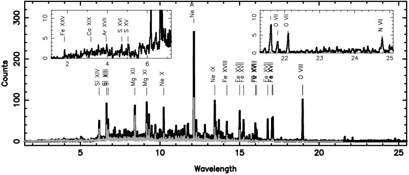
Figure 1: HETGS spectrum of VW Cep, 116 ks exposure. MEG (16433 counts) is the black line, and HEG (5269 counts) the gray. Insets show detail of the HEG spectrum (left) and MEG O VII triplet and N VII region (right).

Figure 1 shows the counts spectrum obtained from the HETGS full exposure. The spectrum is qualitatively typical of coronal sources: a variety of emission lines from highly ionized elements formed over a broad temperature region, from O VII, N VII, Ne IX, and Fe XVII ($\log T\sim 6.3$–$6.7$), up to high temperature species like S XV, S XVI, Ca XIX, and Fe XXV ($\log T\sim 7.2$–$7.8$). It is apparent that iron has a fairly low abundance relative to neon, given the relative weakness of the 15Å and 17Å Fe XVII lines relative to the Ne IX 13Å lines. The observed flux in the 2–25 Å is $8.4\times 10^{-12}\,\mathrm{ergs\,cm^{-2}\,s^{-1}}$, and the luminosity (for a distance of 27.65 pc (Perryman et al., 1997) is $7.7\times 10^{29}\,\mathrm{ergs\,s^{-1}}$.

3 Analysis

3.1 Light and Phase Curves

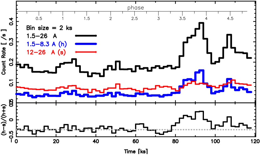
Figure 2: Count rates of VW Cep in 2 ks bins. In the upper panel are light curves extracted from all diffracted photons (1.5-26Å; upper heavy curve), a “soft” band (12-26Å; lower, thinner curve), and a “hard” band (1.5-8.3Å; lower, thicker curve (blue)). The lower panel shows a hardness ratio (solid histogram), and the median of the hardness for the first 70 ks (light dotted line). We defined the non-flare state as the first 80 ks. At the top we show an axis in which the integer part gives the number of rotations and the fractional part is the phase.

The exposure lasted for five revolutions without interruption. Such phase redundancy is important to discriminate intrinsic variability from that caused by rotational or eclipse modulation (for example, see the UV and X-ray monitoring studies of AR Lac, Neff et al. (1989); Huenemoerder et al. (2003b)). Figure 2 shows light curves of diffracted photons (HEG and MEG, orders $-3$ to $3$, excluding zeroth) covering the entire HETGS spectrum as well as for two wide bands covering short (“hard”, 1.5–8.3Å) and long (“soft”, 12–26Å) wavelength regions. The hardness counts ratio (defined as $(hard-soft)/(hard+soft)$) shows that the large increase after 80 ks is probably a flare: proportionally more flux was emitted at shorter wavelengths, which are very sensitive to high temperatures through thermal continuum emission. Conversely, the bump in count rate between 20-30 ks does not show in hardness, and likely is due to rotational modulation.

We assume that flares are hot and will thus show a change in hardness, and that changes in volume alone will primarily show a change in count rate. More complicated scenarios are possible, such as extended loops with temperature gradients rotating in and out of view and causing both hardness and count-rate variability on the time scale of a rotation. However, we know that flares — defined as hot, impulsive events with a gradual decay, in analogy to flares resolved on the Sun — are frequent on most active stars, and we will adopt the assumption as our working hypothesis.

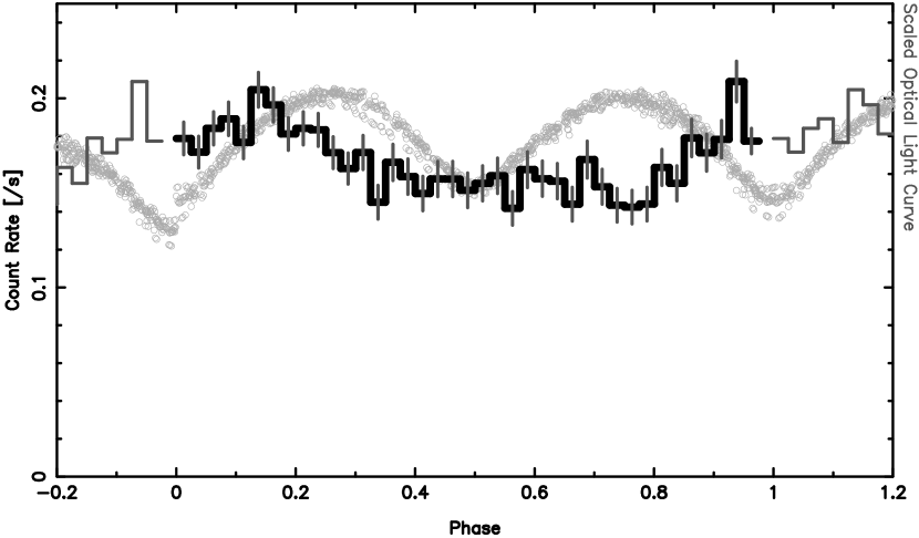
Figure 3: The dark, solid histogram is the phase-folded X-ray count-rate curve of VW Cep, excluding flare times. Bins are $\Delta\phi=0.025$, or 600 s, with a cumulative exposure per bin of 1800 to 2400 s, depending on the phase. Errorbars on the histogram are the $1\sigma$ statistical uncertainties. The gray points are a scaled visual intensity light curve to show the very different character of the optical and X-ray light spatial distributions (Visual photometric data are with permission from T. Pribulla at http://www.astro.sk/$\sim$pribulla/lc/vwcep.dat.)

Rotational modulation is apparent in the phase-folded curve of the non-flare times, which covers about three orbital periods. Figure 3 shows this curve, using the ephemeris of Pribulla et al. (2002). No eclipses are obvious but there is gradual modulation on the orbital period with an amplitude of 20%. The difference between the maximum and minimum, given the $1\sigma$ statistical errors shown, is about $5\sigma$. The visual light curve (Pribulla, Parimucha & Vanko, 2000) has a similar amplitude but is very different qualitatively, having strong minima at phases 0.0 and 0.5, and continuous variability in between (a trademark of W UMa systems). The optical phase modulation is primarily dependent upon the system geometry and inclination.

Without additional information, the X-ray light curve is not sufficient for localizing emission to one star or another. All we can say is that there is some asymmetric distribution, and possible occultation of longitudinally extended structures. It does not appear that there is significant emission from the smaller star, since there is no secondary eclipse at phase 0.0. The X-ray light has a distribution very different from the optical light.

3.2 Velocity Modulation

In the high-resolution spectrum, additional information is available in the line positions which can help localize the emission by means of a determination of the mean radial velocity of the emitting plasma. In any single feature, even the strongest, Ne X (12.1 Å), the line position is poorly constrained in phase bins small enough to sample the orbital velocity. Huenemoerder & Hunacek (2005) showed that the Ne X mean Doppler velocity followed the primary’s orbital radial velocity except for a sharp rise and fall across the secondary eclipse. This “flip-flop” is known as the Rossiter effect (Rossiter, 1924) if it is due to resolution of the rotational velocity profile of the star through occultation of velocity ranges during a transit. Given the low signal level available in a single line, this interpretation was not firm.

We have improved upon that measurement by accumulating signal from many lines and constructing a composite line profile. This mixes resolutions and line shape since long-wavelength lines have higher velocity resolution than shorter wavelengths, but it does have the advantage of increasing signal greatly. Since HEG and MEG have different resolutions and coverage, we kept their composites separate. To avoid blending, we chose only fairly isolated features, and these are flagged in the “Use” column of Table 1 with an “H” or an “M”.

We accumulated spectra into 24 phase bins for each of the HEG and MEG positive and negative first orders (96 distinct spectra). We then transformed about 15 lines in each spectrum from wavelength to a common velocity scale and summed them. Finally, we combined plus and minus orders over a range of phase bins (to further improve the signal) and fit Gaussians to the composite profiles’ cores (defined to be where the counts were greater than the maximum divided by $2e$) separately for each of HEG and MEG. This method is similar to that used by Hoogerwerf, Brickhouse & Mauche (2004). We found that using five phase bins (a running average over $\Delta\phi=0.2$) was adequate to provide enough phase resolution and signal without losing too much sensitivity to velocity changes. To quantify the significance of the fitted velocity centroid, we computed the 90% confidence intervals ($1.6\sigma$) for the velocity.

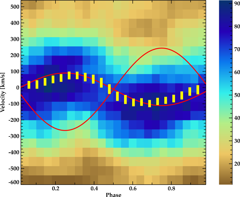
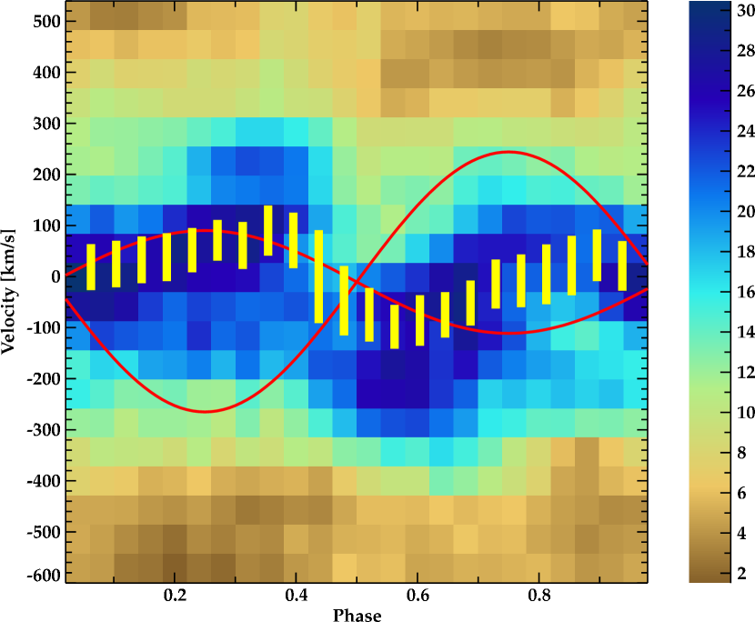
Figure 4: Composite line profile for the MEG spectrum (top) and HEG (bottom). Yellow bars are the 90% confidence intervals of the centroid of the composite profile. The red sinusoidal curves are the center-of-mass velocities of the binary components. The background is an intensity map of the composite profiles’ counts. The bar to the right of each image gives the counts-to-color mapping for the image. The systematic deviations from the primary’s (more massive star) velocity are clear in the HEG for phases 0.5-1.0. The centroids are correlated since they were measured in phase bins of width 0.2. The red curves were also averaged over the same phase intervals as the data.

Figure 4 shows the results. The composite line profiles make the background image, with velocity on the $y$-axis, and phase on the $x$-axis, and the darker shading is for higher intensity as indicated by the color-bar to the right, mapping color to counts. The yellow error bars are the 90% confidence limits of the composite profiles centroid averaged over 5 phase bins ($\Delta\phi=0.2$). The red curves show the stellar center of mass velocities, also averaged over the same phase range as the data.

The composite velocity centroid very closely follows the radial velocity of the primary (more massive) star. The preliminary sharp velocity transition at $\phi=0.5$ seen in neon (Huenemoerder & Hunacek, 2005) is not apparent in the MEG curve, but the background HEG image does have a hint of a transition sharper than that due to the stellar radial orbital velocities.

There are significant systematic deviations from the orbital velocities apparent near $\phi=0.8$. Given the statistical uncertainties shown are 90% ($1.6\sigma$), the deviations from the expected velocity are about $2.5\sigma$ for each grating.

Note that the instrumental resolution is approximately $500\,\mathrm{km\,s^{-1}}$ FWHM at 12Å for the MEG, and about half that for the HEG. We are able to determine centroids to much higher precision ($\sim 25\,\mathrm{km\,s^{-1}}$ for MEG; $\sim 45\,\mathrm{km\,s^{-1}}$ for HEG) because have accumulated signal over multiple profiles, and because each profile is over-sampled by the spacecraft dither which randomizes line placement with respect to pixel boundaries. Hoogerwerf, Brickhouse & Mauche (2004) achieved precision of about $\sim 15\,\mathrm{km\,s^{-1}}$ from MEG spectra, and also quote a statistical verification of the precision of a Gaussian fitted centroid. Also for comparison, Ishibashi et al. (2006) using different techniques on HETGS spectra of Capella, a low-orbital velocity sytem, obtained $3\sigma$ velocity uncertainties of about $20\,\mathrm{km\,s^{-1}}$ which is about $11\,\mathrm{km\,s^{-1}}$ for 90% confidence. It is not surprising that our precision is somewhat less given the lower signal per phase bin and given more velocity smearing in phase for this short period system.

The implications of the velocity centroid variations with regard to geometric distribution of the emitting plasma will be discussed in Section 4.1 in conjunction with light curve variability, emission measure, and density determinations.

3.3 Line Fluxes

Line fluxes, which are required for differential emission measure ($DEM$) analysis, were measured by fitting a the sum of a continuum model and a number of Gaussians to narrow regions of the counts spectra. The parameters of the fits were the Gaussian centroids and fluxes. The continuum and Gaussian widths were determined a priori. For the continuum, we used a plasma model determined iteratively from the emission measure solution (see Section 3.4). For the first iteration, we fit a two-temperature plasma model to relatively line-free regions, as determined by the model and instrument response. Since lines were measurably broader than the instrumental resolution, we determined the amount of excess line width required at one wavelength for a strong, relatively isolated line (Mg XII 8.4Å), then scaled the width with wavelength, under the assumption that the broadening is due to either rotational or orbital effects. However, we simply treated the broadening as a Gaussian, which was adequate for the purposes of obtaining good fits to line fluxes and positions. The excess required was equivalent to about $200\,\mathrm{\,km\,s^{-1}}$ of turbulent broadening.

All fits were done by convolving the model with the instrument response, using effective areas and line-responses made with CIAO tools (mkgarf and mkgrmf; see Section 2). Positive and negative orders were combined dynamically (that is, in memory, with no new counts or response files created on disk), and the HEG and MEG spectra were fit jointly in regions were there were sufficient counts in each.

Line identification and blending were determined iteratively with the $DEM$ solution. Given the plasma model, blended components were added and removed from the fits according to whether the model showed that resolved blends were important or negligible.

The measurement methods used here are similar to those described by Huenemoerder et al. (2003b). All the line fitting was done with scripts programmed in ISIS version 1.2.8.

The resulting counts spectrum and convolved model are shown in detail in Figure 5.

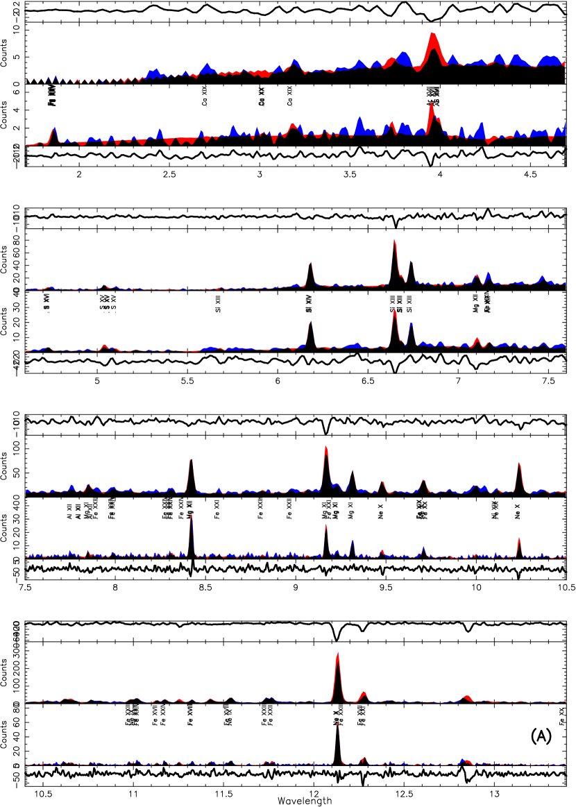
Figure 5: Detailed spectrum and synthetic spectrum from the $DEM$ and abundance fit. The inner two panels of each box show the MEG (upper) and HEG spectra. The counts are shown in dark color (blue), the folded model in lighter color (red). The overlap is filled with black. The very top and bottom panels of each box are counts residuals for each spectrum. Lines from Table 1 are marked. Spectra were binned by two and Gaussian smoothed, except for the 1.7–4.7 Å region where both HEG and MEG were grouped by 4 bins, the 4.6–7.6 Å and $>13$ Å regions where HEG was grouped by 4 bins.

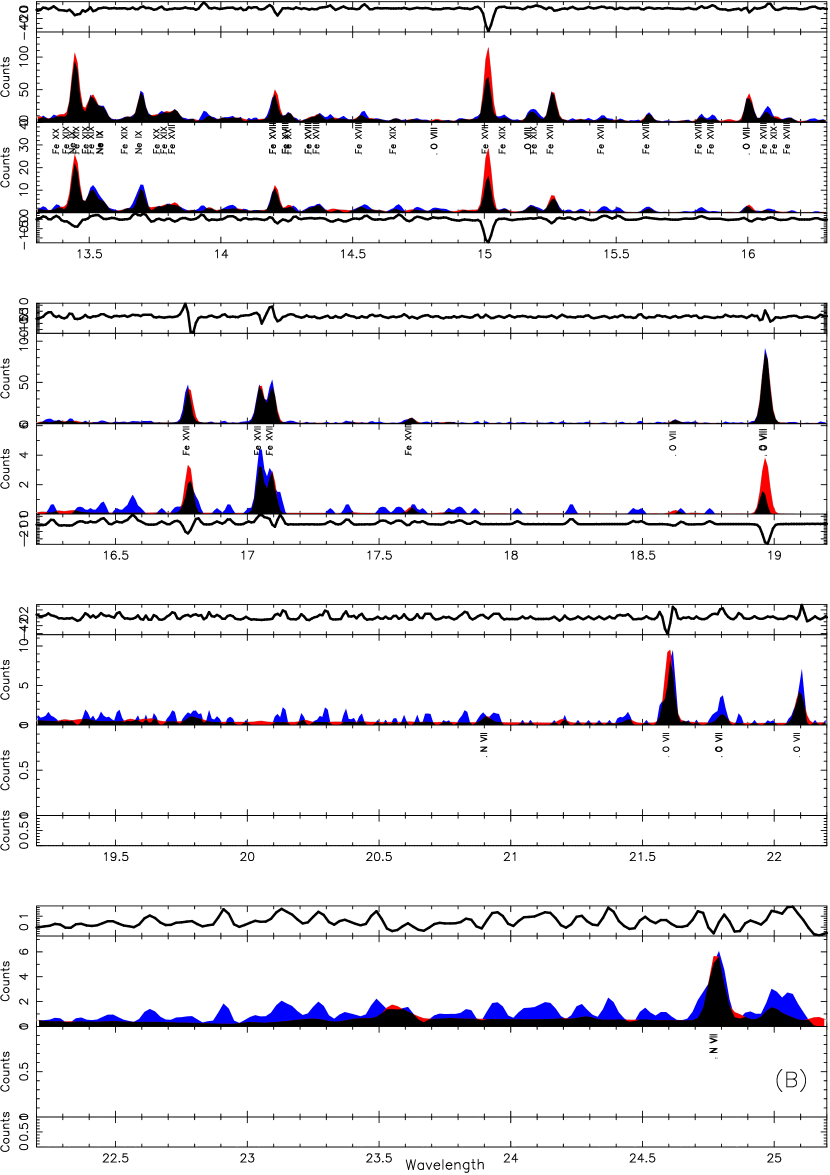
Figure 6: Detailed spectrum, part B; see Figure 5

All the line measurements are given in Table 1. We list more features than were used in analysis. Some were rejected because they had large wavelength residuals and so are misidentified or are strongly blended. Some were rejected because they had large flux residuals and so are misidentified or have poor atomic data. For example, the Fe xvii 15 Å line is nearly always under-predicted, which may be due to deficiencies in the atomic data (Laming et al., 2000; Doron & Behar, 2002; Gu, 2002). Some lines were fit simply to provide a good determination of the flux and wavelength of a nearby “interesting” feature. The “Use” column of Table 1 indicates which lines were used in emission measure reconstruction, or for composite line profiles. The density sensitive He-like triplet inter-combination and forbidden lines were not used in $DEM$ reconstruction.

3.4 Emission Measure

The differential emission measure is a one dimensional characterization of a plasma, and can be defined as $N_{e}^{2}\,dV/dT$, in which $N_{e}$ is the electron density, $V$ is the emitting volume, and $T$ the temperature. The $DEM$ is an important quantity because it represents the radiative loss portion of the underlying heating mechanism. An emission measure can be derived from measurements of line fluxes and some assumptions about the homogeneity and ionization balance of the emitting plasma. Derivation of the emission measure relies on detailed knowledge of fundamental atomic parameters. Even given accurate emissivities, the contribution functions versus temperature are broad so the emission integral cannot be formally inverted. Hence there are many methods to regularize the solution to obtain the emission measure and elemental abundances.

Huenemoerder & Hunacek (2005) used a simple method described by Pottasch (1963), in which the $DEM$ is approximated by a ratio of line luminosity to average line emissivity at the temperature of the maximum emissivity. Here we improve upon that by simultaneously fitting the $DEM$ and abundances using a method similar to that described by Huenemoerder et al. (2003b), who also discussed some of the caveats of emission measure reconstruction and gave relevant citations. Briefly, the relation between emissivity and flux is an ill-posed problem. To obtain a unique solution, under assumptions of the model, a regularization term of some form must be included. Here we have replaced explicit smoothing of the $DEM$ in our prior work with a regularization term, so that the functional form of the statistic we minimize is

$$\chi^{2} =\sum_{l}\frac{1}{\sigma_{l}^{2}}\left[L_{l}-A_{Z(l)}\sum_{t}{\delta_{t}\epsilon_{lt}D_{t}}\right]^{2}+qP(D),$$ (1)

in which $l$ is a spectral feature index and $t$ is the temperature index. The measured quantities are the line luminosities, $L_{l}$, with uncertainties $\sigma_{l}$. The a priori given information are the emissivities, $\epsilon_{lt}$ as defined by Raymond & Brickhouse (1996), $\delta_{t}$ is the logarithmic bin size, and the source distance (which is implicit in $L$). The minimization provides a solution for the differential emission measure, $D$, and abundances of elements $Z$, $A_{Z}$. To naturally constrain the $DEM$ to be positive, we actually fit $\ln D_{t}$. $P(D)$ is a regularization term (or “penalty function”) which is only a function of the model, and $q$ is a scale factor which specifies the relative importance of the regularization. For $P$, we used the sum-squared second derivative of the $DEM$ with respect to $\log T$, and a multiplier to make the two terms of the statistic comparable. This form imposes a minimum smoothness on the solution; the $DEM$ cannot have large changes in curvature. We did not impose any regularization on the abundances, since we have no intuitive bias on their functional form.

The $DEM$ fitting was done with custom software in ISIS. While ISIS has no built-in $DEM$ reconstruction, it does have sophisticated plasma database access and evaluation functions permitting efficient lookup and computation of emissivities. It also provides for user-defined fit functions and statistics, which made it straightforward to develop a $DEM$ model within its fitting and modeling infrastructure.

As an initial guess, we assumed cosmic abundances and a boxcar $DEM$; the amplitude of the central temperature region was chosen to approximately produce the observed line counts, and the ends were set to a very low value. The reason for leaving the $DEM$ at the temperature extrema low is that the $DEM$ is not well constrained physically there by lines, but the hot portion does strongly affect the continuum. Hence, we preferred a solution in which emission weights are increased only if required by the fit to lines alone. The normalizations outside our regime of temperature sensitivity, roughly $\log T=6.4$ (O vii) to $7.8$ (Fe xxv; the tail of Si xvi), were artificially constrained to have negligible emissivity. The line-to-continuum ratio was fit post facto by scaling the normalization of the $DEM$ and abundances.

The model $DEM$ was obtained iteratively. For each trial $DEM$, we generated a new continuum model and re-fit the lines. After the second such iteration, we reviewed line residuals and excluded those which were very large (greater than $3\sigma$), under the assumption that they were misidentified or blended. The final fit included only the selected lines, and was post facto renormalized to reproduce the observed line-to-continuum ratios in the 8-11 Å range. The line fluxes predicted by the $DEM$ and abundance model are listed in Table 1, along with the residuals from the parametric fit, and their $\delta\chi$ value (last three columns). The “Use” column flags lines used in the $DEM$ reconstruction with an “E”. Due to the iterative nature of the model, the measured line fluxes are slightly dependent upon the $DEM$ solution through the definition of the continuum.

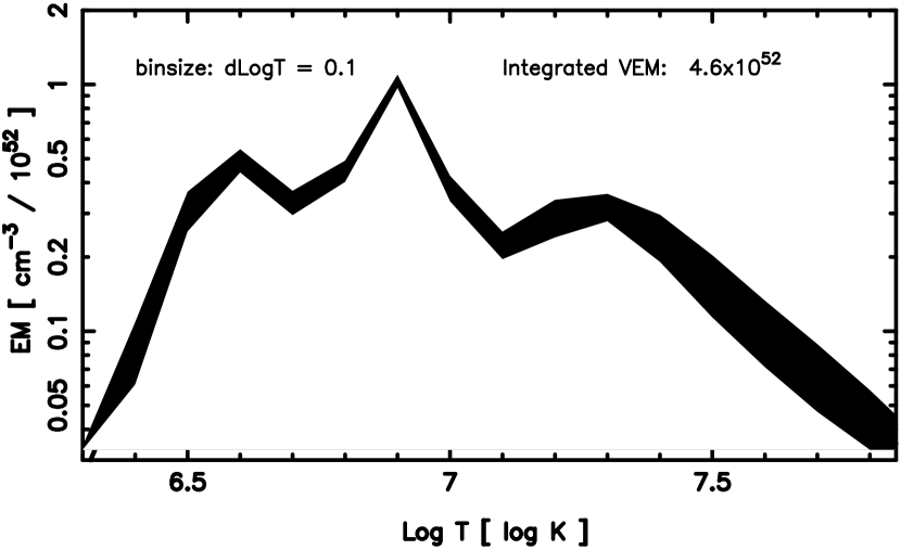
Figure 7: In this reconstructed emission measure distribution, the width of the filled region is the 1-standard-deviation range as determined from a Monte-Carlo run in which the observed line fluxes were randomized according to their statistical uncertainty. The fit is physically unconstrained at the highest and lowest temperatures plotted, but was artificially constrained to have a negligible value at the extrema. The integrated emission measure is about $4.6\times 10^{52}\,\mathrm{cm^{-3}}$.

Figure 7 shows our final emission measure (integrated over logarithmic bins of width 0.1 dex), using the Astrophysical Plasma Emission Database (APED, Version 1.3.1) for line emissivities (Smith et al., 2001), the ionization balance of Mazzotta et al. (1998), and Solar abundances from Anders & Grevesse (1989). The envelope shown was determined by computing the deviation in solutions over a Monte-Carlo run of about 100 fits in which the line fluxes were varied according to their measured statistical uncertainties, assuming a Gaussian distribution about their fitted values. This assumption would actually result in an enlarged uncertainty bounds, since the data are an estimate of the true mean, and the random perturbation would sometimes be toward the true mean, and sometimes away, perhaps further than the the measured uncertainty and truth would allow.

Other sources of systematic error, the uncertainties in the atomic physics and in the instrumental calibration, were not included, and probably accounts for a similarly sized envelope. While systematic uncertainties in atomic data are difficult to incorporate explicitly, Huenemoerder et al. (2003b) applied an approximate method, in which they set a global lower limit on the line flux uncertainty of 25% (regardless of the statistical uncertainty) and repeated the $DEM$ reconstruction. They found a similar shaped distribution, but proportionally larger uncertainty. The important quantity for understanding coronal activity is the overall shape of the $DEM$, which seems reliable under the current assumptions and calibration uncertainties.

There is sharp structure in the $DEM$ with a large peak at $\log T=6.9$, a second peak at 6.6, and hot tail from about 7.2 to 7.8. This is qualitatively similar to the simple provisional $DEM$ of Huenemoerder & Hunacek (2005), but with sharper structure as expected from an iterative solution.

Figure 8: The reconstructed abundances relative to Solar are plotted against their first ionization potential (FIP). Error bars are the one standard deviation range from the Monte-Carlo emission measure and abundance reconstruction, or in the cases of Ni and Ca, from a post facto fit of abundances given the $DEM$.

The fitted coronal abundances, relative to Solar (since we do not know the stellar photospheric values), are shown in Figure 8. The uncertainties are the $1\sigma$ range as determined by the Monte-Carlo iteration, except for Ni and Ca. The latter two were not included in the $DEM$ solution since they were weak and were not fit with parametric profiles as were the strong lines (and so they do not appear in Table 1). Instead, we fit them post facto by using the $DEM$ and abundance solution to define a plasma model, then adjusted the abundance of Ca by minimizing the residuals between the binned counts and synthetic spectrum in the Ca XIX He-like triplet near 3.2 Å as a function of Ca abundance. There is a blend of Ar XVII here, but given the $DEM$, it is expected to be about an order of magnitude weaker than Ca. For Ni, we similarly fit the Ni XIX lines at 14.043 and 14.077 Å, and Ni XIX 12.435 Å. In each region, blended Fe lines had model fluxes 5-10 times weaker than the nickel lines. The Ca abundance uncertainty is large because there are few counts and a relatively strong continuum. The Ni has smaller uncertainty because there are more counts and weaker continuum.

3.5 Density

The helium-like triplets are well known as density sensitive diagnostics, particularly the ratio of the forbidden ($f$) to inter-combination ($i$) line fluxes, commonly known as the $R$-ratio, $R=f/i$ (Gabriel & Jordan, 1969; Porquet & Dubau, 2000; Porquet et al., 2001; Ness et al., 2001). A mildly temperature sensitive diagnostic is the $G$-ratio, which is the sum, $f+i$, divided by the resonance line ($r$) flux. The critical density increases with atomic number. In the HETGS range, the ions of interest for coronal diagnostics are O VII, Ne IX, and Mg XI.

The O VII triplet ratios are relatively straightforward to determine since the lines are well separated, unblended, and the continuum is low. Ne IX is a difficult case since it is blended with several line of Fe XIX and Fe XX, in addition to having a significant continuum. Ness et al. (2003a) performed a thorough analysis of this region in Capella at different resolutions, and showed that HEG resolution is necessary for accurate modeling. The Mg XI region is of intermediate difficulty; it contains blends with the Ne X Lyman-like series, which converges near the inter-combination line. Neon is often overabundant in stellar coronae, making the contribution possibly significant.

We have determined $R$ and $G$ ratio confidence contours for O VII and Ne IX by directly fitting the line ratios to the spectra. Fits were done similarly to the lines (see Section 3.3), but with the addition of parameter functions to define fit-parameters for the ratios themselves.

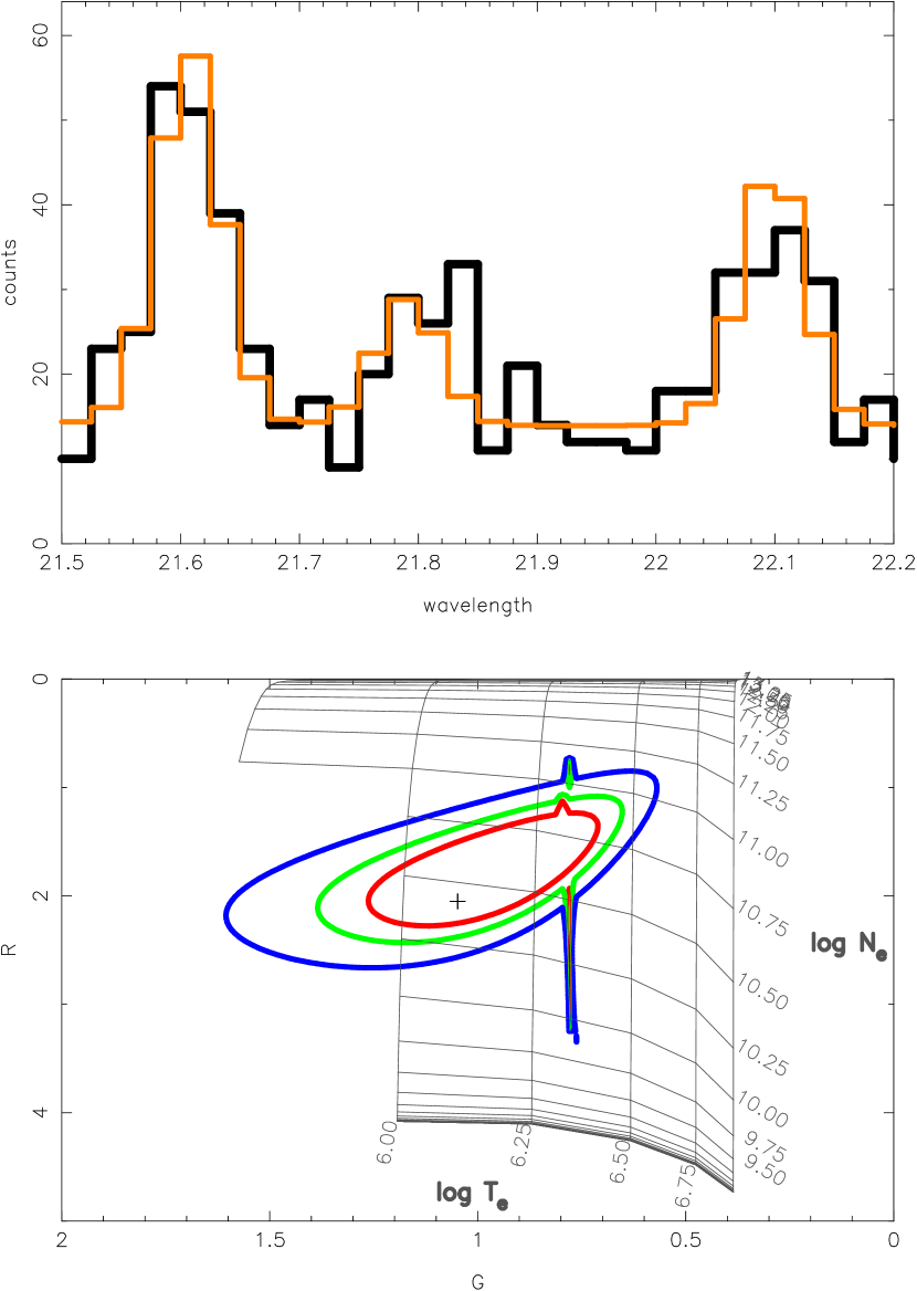
Figure 9: The LETGS O VII spectral region (top, dark histogram), model (top, light histogram), and the confidence contours (bottom, colored ovals) for the $G$ and $R$ ratios. The theoretical isothermal, isodensity $G-R$ ratio grid is plotted in gray, and labeled with the logarithmic density and temperature values. The best fit density is about $\log N_{e}=10.5$. The HETGS data give a similar result, but with larger contour regions. (The vertical spike in the contours is a numerical artifact.)

Figure 9 shows the result for oxygen. Here we have decided to use the LETGS data (observation ID 2559), since it has better signal at O vii, and the contours are smaller than for the HETGS. Though at a different epoch, the solutions from HETGS and LETGS are equivalent. We have plotted the axes reversed, since the temperature and density increase inversely with the ratios. The contours show the one-, two-, and three-sigma confidence intervals, with the best fit marked with a “plus” sign. The underlying grid shows the theoretical ratios’ lines of constant temperature and density (density dependent tables are from Brickhouse, private communication). We also show the counts spectrum and best fit model. The $R$ ratio contours clearly show a density above the low-density limit; the best fit value is $\log N_{e}=10.5$, with the $1\sigma$ confidence interval ranges from 10.3 to 10.8. The $G$-ratio spans a broad range but is not inconsistent with the reconstructed $DEM$.

For the Ne IX region, we included nine resolved lines of Fe XVII, Fe XIX, and Fe XX. There is an unresolved blend of Fe XIX and Fe XX with the inter-combination line. From fits to the neighboring lines, the $DEM$ model and APED, we can estimate the contribution of iron to the Ne $i$-line of about 15%. This was included as a frozen component in the ratio fit. We show the counts, Ne IX, and Fe model in Figure 10 for both HEG and MEG, since resolution is critical. The figure also shows the model continuum, and Table 1 flags the resolved iron blends included.

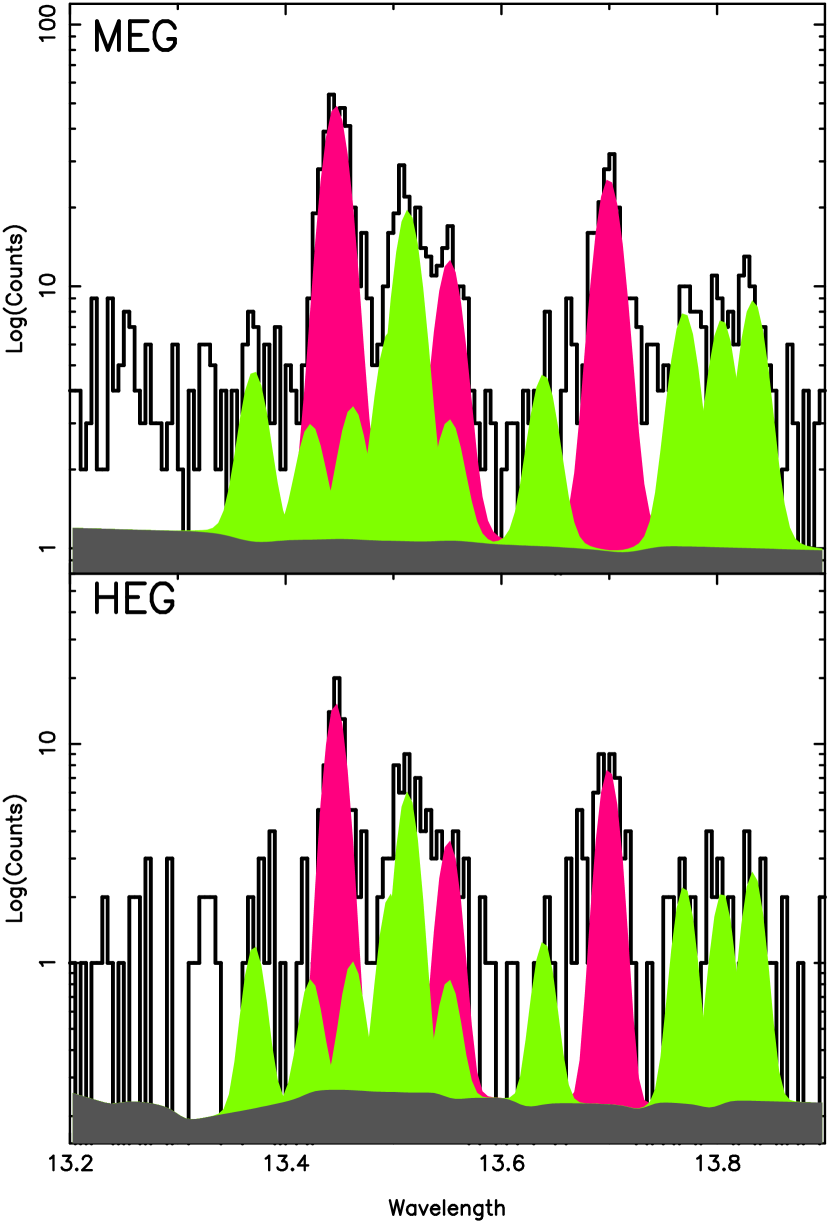
Figure 10: Ne IX region for MEG (top) and HEG (bottom), showing the counts (dark histogram), the Ne IX components (red-filled Gaussians), the iron components (green-filled Gaussians), and the continuum model (gray-filled region). The relative intensity of the iron line blended with the Ne IX inter-combination line was determined from neighboring iron lines. Note that the counts scale is logarithmic.

For the unresolved blends, we give the identifying information from the APED, which labels lines uniquely by the element, ion, upper ($u$), and lower ($l$) levels: Fe XIX $\lambda 13.551$ ($u=65$, $l=1$); Fe XX $\lambda 13.535$ ($u=109,107$, $l=7$), $\lambda 13.558,13.565$ ($u=110,109$, $l=8$).

In Figure 11, we show the resulting $G-R$ contours and spectra with best-fit model. Here, it is not clear that the density is above the critical value; the best fit is $\log N_{e}=11.25$, and the one-sigma range is 10.0-11.4. The $G$-ratio contours extend to low temperatures, but the range is not inconsistent with the $DEM$.

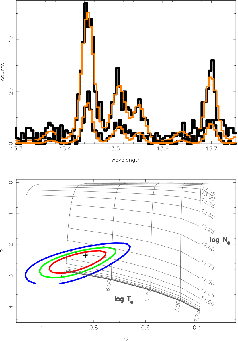
Figure 11: Ne IX spectral region (top, dark histogram), model (top, light histogram), and the confidence contours (bottom, colored ovals) for the $G$ and $R$ ratios. The theoretical isothermal, isodensity $G-R$ ratio grid is plotted in gray, and labeled with the logarithmic density and temperature values. The best-fit density is about $\log N_{e}=11.25$.

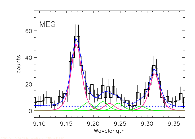
Figure 12: Mg XI region for the MEG, showing the counts (dark histogram), And individual ionic components as smooth curves: Mg XI (red), Ne X and Fe  (green)

We also fit the Mg XI ratios. The ratio and uncertainty gives $R=2.7\pm 0.5$. The theoretical low-density ratio is 2.9. Hence, we are well below the limit of density sensitivity (the critical density is about $\log N_{e}=13$). We included the high-$n$ Ne X Lyman-like series and iron blends in the triplet region (Testa, Drake & Peres, 2004), which we show in Figure 12.

4 Discussion

There is no question that coronal activity saturates at short periods, and that super-saturation occurs at even shorter periods. Why saturation occurs is still an open question among hypotheses of dynamo suppression by tidal interactions, coronal stripping via Coriolis forces, filling factors near unity, or other effects. With high resolution X-ray spectra, we cannot yet solve this problem, but we can provide additional details from individual case studies. We can make several deduction from the VW Cep light curves, line velocities, emission measures, and density diagnostics. We will also consider the similar super-saturated W UMa system, 44 Boo.

4.1 Coronal Geometry

From visual inspection of the VW Cep X-ray light curve, we see that X-rays vary in brightness quasi-sinusoidally at the period of the binary with a modulation of about 20%. The shape is very different from the optical curve, which is determined primarily by the geometric configuration of two stars with nearly equal surface brightnesses (tidally distorted spheroids which undergo partial eclipses) and secondarily by inhomogeneous brightness distributions (gravity darkening and starspots). Since we do not see obvious eclipses in X-rays (which could have a phase duration of about 0.2), we infer that the regions obscured probably do not contribute significant X-ray emission within our detection sensitivity. Since the inclination is $63^{\circ}$, and the primary has about twice the radius of the secondary, the regions covered are roughly the southern hemispheres of each star. The north-polar region of each star is always visible, roughly within co-latitude of $30^{\circ}$, so any emission from this region on either star will contribute a constant emission component (within projected area affects). The non-uniform emitting material can thus be roughly constrained to latitudes of $0-60^{\circ}$, in one hemisphere only, with more emission measure seen near phase 0 (larger star in front).

If we now consider the X-ray composite radial velocity curve, we can rule out significant emission from the secondary (smaller) star, at the limit of about 30%. The ratio of photospheric surface areas is about 2:1. If we had 30% of the X-ray line flux originating from the secondary, it would have been apparent in the composite line profiles, but we do not see it (see Figure 4). We explored the limits of the secondary’s signature in the composite profiles through simulations. We simulated spectra using the same model emission measure for each star, but doing a weighted sum at each phase, with each spectrum redshifted according to the phase. We used the same exposure times from each bin of the observed phase curve as well as ones 100 times larger. We considered relative weights, primary to secondary of 0.7:0.3 (the ratio of areas), 0.8:0.2, and 1:0. After the simulated data were produced, the composite lines were formed and measured in exactly the same way as for the observation.

For the 0.7:0.3 weighting, modulation in the composite centroid is reduced to an undetectable size. For 0.8:0.2, modulation is reduced by about 50%, to about the maximum deviation seen in the HEG near phase 0.8. For all emission from the primary, the curve follows the primary radial velocity, as expected. Thus, we find most emission at most phases can be attributed to the primary. At some phases, approximately 0.75–1.0, we may have about 20% from the secondary. Since there is no apparent eclipse of the secondary (at phase 0.0, the primary eclipse), the emission from the secondary must be at high latitudes on the trailing hemisphere, but not polar or we would have a larger velocity centroid perturbation near phase 0.25.

We can next apply emission measure and density information to estimate coronal extent, under some simplifying assumptions about the emitting plasma’s geometry. If we assume that the 20% light curve intensity modulation is caused by a random distribution of identical coronal structures of constant cross-section, then we can have about 25 structures, based purely on counting statistics. Using the scaling relation of Huenemoerder, Canizares & Schulz (2001), an integrated emission measure of $4.6\times 10^{52}\,\mathrm{cm}^{-3}$ and a density range of $\log N_{e}=10.5$ to $11.25$, and assuming all emission comes from the primary of radius $0.9\,R_{\odot}$, then the structure height is about 0.06 to 0.2 stellar radii. Such a corona would thus be fairly compact, which is self consistent; if it were very extended, flux modulation could be much less. A single such structure could have a height from 0.2 to 0.6 stellar radii and could probably be placed to create the same intensity modulation. We prefer the multiple structure hypothesis, but this is by no means a unique requirement of the data. If we spread the emitting volume more uniformly over a hemisphere, then for the above density range the fractional height is 0.02 to 0.03. We probably have a compact, polar corona.

Gondoin (2004b) reported an X-ray eclipse seen XMM-Newton light curves obtained 10 months prior to the CXO observations and concluded that both components were X-ray emitters. If the dip in XMM-Newton rate were really an eclipse, then this would indicate rather large and rapid changes in coronal structure. The XMM-Newton observation, however, did not cover a single continuous orbit, and the dip is offset from phase 0.0, so the interpretation is not definitive. Also contrary to our results, Gondoin (2004b) derived loops quite large in comparison to the stellar radii (20-80%), but admittedly by methods which are not self-consistent.

4.2 Temperature Distribution, Heating, Opacity

The differential emission measure (Figure 7) is similar to other active stars, being highly structured and spanning a broad range in temperature. Sanz-Forcada, Brickhouse & Dupree (2002, 2003) show a large collection of $DEM$ distribtions with a variety of peaks, bumps, and tails. In our analysis, we included the flare times and this no doubt produces the bump above $\log T=7.1$, similarly to the results for II Peg (Huenemoerder, Canizares & Schulz, 2001) and Proxima Cen (Güdel et al., 2004), which were modeled at different activity levels.

The most prominent peak in the VW Cep $DEM$ is well defined and narrow, with a slope approximately proportional to $T^{4}$. Such a feature has also been observed in other stars of different types (Brickhouse et al., 2000; Sanz-Forcada, Brickhouse & Dupree, 2002). The $DEM$ can give us some insights into the underlying physics. A possible interpretation of this recurrent feature is linked to the spatial location and temporal distribution of coronal heating. Testa, Peres & Reale (2005) have proposed a hydrodynamic model of loops undergoing pulsed heating at their foot-points, which is able to reproduce the presence of a peak and the steep rise of the $DEM$ observed in these active stars. Whatever the mechanism, the heating in VW Cep does not look radically different from other coronal sources, at least as manifested in the $DEM$.

The abundances do not show any strong trend with the first ionization potential (FIP). While Ar looks unusually abundant in Figure 8, the statistical uncertainty is large. Furthermore, the measurement is also subject to systematic uncertainty in placement of the continuum. The Ar abundance is probably not significantly different from Ne. The overall distribution looks very similar, for example, to that of the RS CVn binary, AR Lac (Huenemoerder et al., 2003a). The Ne:O ratio which we derived from the iterative emission measure and abundance reconstruction is $0.35\pm 0.03$. This is comparable to the rather robust active star mean of $0.41$ found by Drake & Testa (2005) from temperature-insensitive line ratios. From the abundance analysis, we again have no reason to think that the corona of a W UMa system, though super-saturated, differs from other coronally active stars.

We examined line ratios which have been used for opacity diagnostics. Fe xvii has been problematic, because the ratios systematically differ from theoretical values (Laming et al., 2000; Doron & Behar, 2002; Gu, 2002). VW Cep is no exception; its Fe xvii 15.01 Å line is over-predicted. We find no significant differences in ratios from typical optically thin values shown in Testa et al. (2004) or Ness et al. (2003b).

4.3 Comparison to 44 Boo

44 Boo is a contact binary system which is very similar to VW Cep, having similar period, mass ratio, and spectral types. Its fundamental characteristics are given by Hill, Fisher & Holmgren (1989) and a velocity curve by Lu, Rucinski & Ogłoza (2001). Brickhouse, Dupree & Young (2001) have analyzed HETGS spectra and concluded that most emission is at high latitudes, compact, that there is a very compact emitting region on the smaller star (the secondary) which causes a very brief dip in X-ray brightness when it momentarily rotates out of view, and a larger emitting region near the pole of the primary which gives rise to a quasi-sinusoidal brightness modulation, but which isn’t eclipsed. Gondoin (2004a) presented XMM-Newton observation of 44 Boo which covered on orbital period. Based on the absence of eclipses, he concluded that the corona must be extended, though he presented other arguments which led to compact loops.

Using the same techniques applied to VW Cep, we have extracted the X-ray light and phase curves and a composite line velocity curve from the same HETGS observation used by Brickhouse, Dupree & Young (2001) (Observation ID 14). The light curve in Figure 13 shows three flares. The rise in the final 10 ks, identified as a flare by Brickhouse, Dupree & Young (2001), shows no increase in hardness, so we accept it into the phased curve.

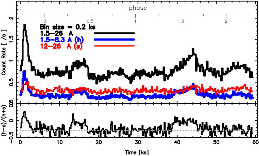
Figure 13: Count rates of 44 Boo in 200 s bins. In the upper panel are light curves extracted from all diffracted photons (1.5-26Å; upper heavy curve), a “soft” band (12-26Å; lower, thinner curve), and a “hard” band (1.5-8.3Å; lowest, thicker curve). Near the top is an axis giving the orbital phase plus a rotation count. The lower panel shows a hardness ratio (solid histogram), and the median of the hardness for the middle flat section (light dotted line). We defined the three high hardness regions as flares and excluded them from the phase curve (0-5, 12-18, and 38-46 ks).

Our phased X-ray light curve (Figure 14) is qualitatively different from Brickhouse, Dupree & Young (2001).

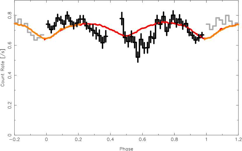
Figure 14: The dark, solid histogram is the phase-folded X-ray count-rate curve of 44 Boo, excluding flare times. Bins are $\Delta\phi=0.025$, or 462 s, with a cumulative exposure per bin of about 460 to 1400 s, depending on the phase. The gap near phase 0.4 is from missing data, due to flare-time filtering. The smooth curve is a scaled $B$ light curve to compare optical and X-ray light spatial distributions. Photometric $B$ data are from T. Pribulla (http://www.astro.sk/$\sim$pribulla/lc/44boo.jpg.)

Since W UMa stars undergo period variations, we were careful to reference the ephemeris to light-curves from the same epoch (Pribulla et al., 2001). We also obtained a $B$ photometric light curve from the same epoch and scaled it to arbitrary relative intensity to display over the X-ray curve. We do find strong evidence for the primary eclipse in the broad dip in X-ray flux in good correspondence with the $B$ intensity. The rest of the curve is qualitatively similar to the VW Cep X-ray curve (Figure 3), having a rather broad depression with no obvious eclipse. The gap beginning near phase 0 is due missing data due to the exclusion of flares. We do not find a very narrow dip nor require a very small near-polar emitting region as hypothesized by Brickhouse, Dupree & Young (2001). These differences are probably primarily due to our forming the histogram in phase bins, weighting the counts by the exposure function (which ranges from zero to 2 ks), and in our flare discrimination using a hardness ratio.

Figure 15 shows our composite line profiles and centroid, which is qualitatively similar to the velocity curve of Brickhouse, Dupree & Young (2001).

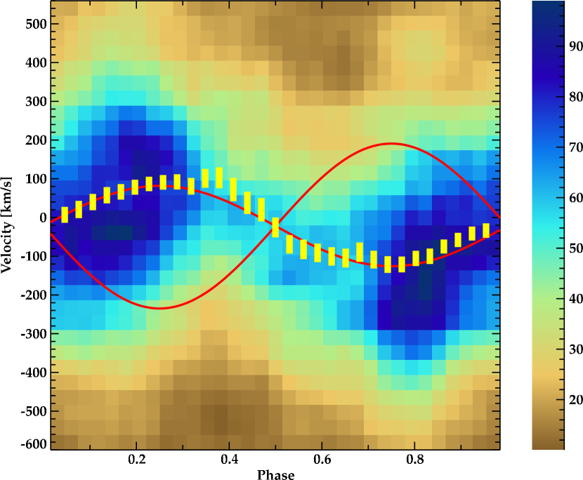
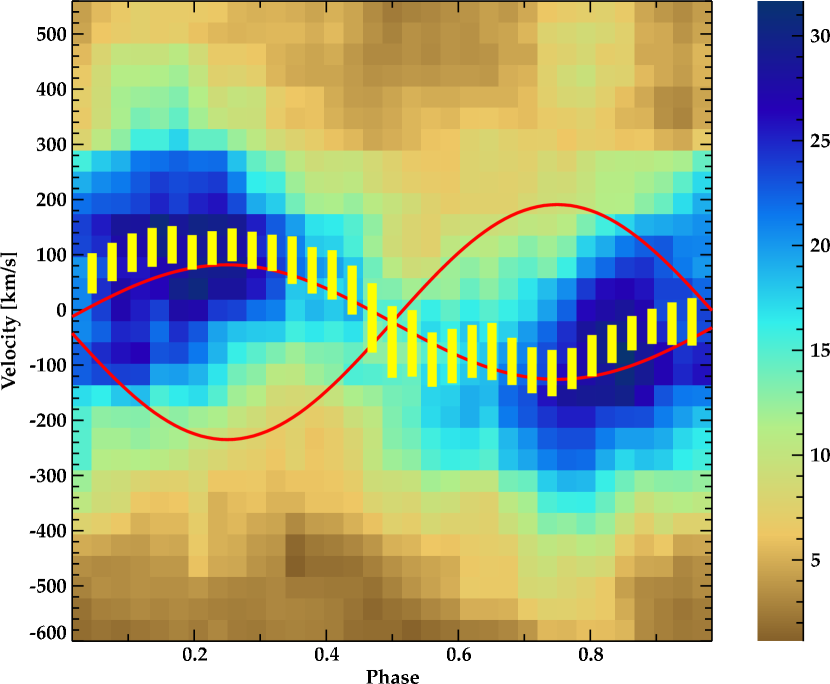
Figure 15: Composite line profile for the MEG spectrum (top) and HEG (bottom) for 44 Boo. Yellow bars are the 90% confidence intervals of the centroid of the composite profile. The red sinusoidal curves are the center-of-mass velocities of the binary components. The background is an intensity map of the composite profiles’ counts. The bar to the right of each image gives the counts-to-color mapping for the image. The centroids are correlated since they were measured in phase bins of width 0.2. The red curves were averaged over the same intervals.

The primary clearly dominates the composite line centroid. However, the distortions and wings also hint at some contribution from the secondary, particularly between phases 0.6–0.9 where the centroid is systematically shifted to more positive velocities. The secondary cannot contribute as much as half the light, however, or the composite profile centroid would be strongly biased toward zero. Given the presence of the primary eclipse, the broadening in the profile wings, slight distortions in the HEG centroid, and simulations, we estimate that the secondary contributes no more than about 20% of the X-ray flux during some phases.

Were it not for the primary eclipse, the 44 Boo situation would be very much like VW Cep: quasi-sinusoidal light curve with a minimum near phase 0.5, 20% contribution from the secondary at some phases. 44 Boo is at a slightly higher inclination than VW Cep, $73^{\circ}$ vs. $63^{\circ}$. This does give it a higher probability of eclipsing compact coronal emission concentrated at high latitudes. On the other hand, it is highly possible that the size and location of the coronal emission migrates, as do the photospheric spots (see, for example, Hendry & Mochnacki (2000)). At future epochs, it is possible that VW Cep will show X-ray eclipses.

5 Conclusions

Super-saturation, at least in the cases of VW Cep and 44 Boo, appears to be manifested in small area of coverage by compact, near-polar structures. Given roughly a factor of two for coronal structures occurring in only one hemisphere, and a factor of two in expected emission per area (the secondary is weak relative to the primary), the X-ray flux can be significantly depressed below the saturated limit of $L_{\mathrm{x}}/L_{\mathrm{bol}}\sim 10^{{}^{-3}}$. Why this occurs is still unexplained, but we favor the general scenario of (Stȩpień, Schmitt & Voges, 2001) which forms polar, but compact, structures.

Given the small area of corona on the secondary, we predict that the secondary’s coronal signature be highly changeable with phase over different epochs. This would show as changes in the depth of primary eclipse and phase of perturbation in the velocity profile. The HETGS is the only X-ray spectrograph currently capable of making these measurements. Obtaining high signal-to-noise per phase bin is of utmost importance to surface geometry reconstruction techniques. Further multi-orbit spectroscopy of these or other short period systems is certainly important to determination of transient or common features. A factor of 10 increase in exposure would permit line profile diagnostics in a single line (Ne x) and greatly facilitate modeling.

Table 1: Line Measurements

Mnemonic	Use	Ion	$\overline{\log T}$	$\lambda_{t}$	$\lambda_{o}$	$f_{l}$	$f_{t}$	$\delta f$	$\delta\chi$
Fe25HeLa	E	Fe xxv	7.81	1.861	1.867 (4.5)	3.10 (1.88)	2.24	0.86	0.5
Ar17HeLar	-	Ar xvii	7.36	3.949	3.948 (15.0)	0.34 (0.54)	2.12	-1.78	-3.3
Ar17HeLai	-	Ar xvii	7.31	3.968	3.970 (3.5)	1.75 (0.79)	0.60	1.15	1.5
S16HLbB	-	S xvi	7.53	3.992	3.995 (8.6)	0.84 (0.71)	0.50	0.34	0.5
S16HLa	E	S xvi	7.57	4.730	4.730 (6.7)	2.57 (0.86)	2.31	0.26	0.3
S15HeLar	E	S xv	7.20	5.039	5.040 (2.5)	4.40 (1.20)	4.06	0.34	0.3
S15HeLai	E	S xv	7.16	5.065	5.072 (5.6)	1.47 (1.05)	0.98	0.49	0.5
S15HeLaf	E	S xv	7.17	5.101	5.106 (6.0)	2.95 (1.20)	1.43	1.52	1.3
Si13HeLb	E	Si xiii	7.06	5.681	5.688 (5.5)	1.90 (1.10)	1.61	0.28	0.3
Si14HLa	EHM	Si xiv	7.39	6.183	6.183 (1.0)	9.00 (0.83)	8.72	0.28	0.3
Si13HeLar	EH	Si xiii	7.03	6.648	6.647 (0.7)	14.72 (1.00)	13.71	1.01	1.0
Si13HeLai	-	Si xiii	6.99	6.687	6.687 (2.5)	2.91 (0.59)	2.70	0.21	0.4
Si13HeLaf	-H	Si xiii	7.01	6.740	6.739 (0.8)	8.58 (0.75)	5.73	2.85	3.8
Mg12HLb	E	Mg xii	7.22	7.106	7.107 (2.7)	2.46 (0.46)	2.91	-0.45	-1.0
Al13HLaB	-	Al xiii	7.36	7.171	7.171 (1.7)	3.03 (0.50)	2.07	0.96	1.9
Al12HeLar	E	Al xii	6.98	7.757	7.758 (2.2)	3.30 (0.64)	0.99	2.30	3.6
Al12HeLai	-	Al xii	6.89	7.805	7.804 (7.1)	0.59 (0.49)	0.35	0.24	0.5
Mg11HeLb	E	Mg xi	6.87	7.850	7.853 (2.5)	3.19 (0.73)	2.77	0.42	0.6
Al12HeLaf	E	Al xii	6.89	7.872	7.872 (—)	0.34 (0.40)	0.96	-0.62	-1.6
Fe23w7.90	E	Fe xxiii	7.24	7.901	7.899 (3.7)	2.77 (0.63)	0.33	2.44	3.9
Fe24w7.986	-	Fe xxiv	7.43	7.986	7.972 (3.4)	1.39 (0.68)	0.97	0.41	0.6
Fe24w7.996	E	Fe xxiv	7.43	7.996	7.992 (5.0)	1.72 (0.64)	0.50	1.22	1.9
Fe24w8.28	E	Fe xxiv	7.40	8.285	8.285 (—)	0.58 (0.56)	0.20	0.38	0.7
Fe23w8.30	E	Fe xxiii	7.25	8.304	8.302 (4.0)	1.66 (0.59)	1.20	0.45	0.8
Fe24w8.32	E	Fe xxiv	7.42	8.316	8.316 (—)	1.38 (0.57)	1.09	0.29	0.5
Fe24w8.38	-	Fe xxiv	7.40	8.376	8.369 (—)	1.39 (0.51)	0.43	0.96	1.9
Mg12HLa	EHM	Mg xii	7.19	8.422	8.421 (0.6)	24.46 (1.41)	22.53	1.93	1.4
Fe21w8.57	E	Fe xxi	7.06	8.574	8.574 (2.9)	3.13 (0.85)	1.05	2.08	2.5
Fe23w8.81	E	Fe xxiii	7.23	8.815	8.815 (—)	1.94 (0.66)	1.26	0.68	1.0
Fe22w8.97	-	Fe xxii	7.13	8.975	8.983 (6.8)	3.22 (0.73)	1.57	1.65	2.3
Mg11HeLar	EHM	Mg xi	6.83	9.169	9.169 (0.7)	23.78 (1.50)	23.14	0.64	0.4
Fe21w9.19	-	Fe xxi	7.07	9.194	9.200 (3.3)	4.17 (0.86)	0.78	3.39	3.9
Mg11HeLai	-	Mg xi	6.80	9.230	9.230 (4.1)	4.72 (0.82)	3.77	0.95	1.2
Mg11HeLaf	-HM	Mg xi	6.81	9.314	9.314 (0.9)	12.81 (1.22)	11.04	1.77	1.5
Ne10HLd	E	Ne x	7.01	9.481	9.479 (1.8)	5.68 (0.86)	3.12	2.56	3.0
Fe19w9.69	-	Fe xix	6.93	9.695	9.681 (2.6)	2.43 (0.67)	1.00	1.43	2.1
Ne10HLg	EHM	Ne x	7.00	9.708	9.708 (1.3)	9.18 (1.00)	7.10	2.07	2.1
Fe20w9.73	-	Fe xx	7.00	9.727	9.742 (2.6)	0.93 (0.62)	0.96	-0.03	-0.1
Ni19w10.11	E	Ni xix	6.84	10.110	10.108 (2.8)	3.67 (0.84)	0.86	2.82	3.4
Fe20w10.12	-	Fe xx	6.99	10.120	10.134 (—)	1.09 (0.63)	1.08	0.02	0.0
Ne10HLb	EHM	Ne x	6.99	10.239	10.239 (0.8)	19.50 (1.45)	22.77	-3.27	-2.3
Fe23w10.98	E	Fe xxiii	7.24	10.981	10.978 (2.3)	5.78 (1.22)	6.55	-0.77	-0.6
Ne9HeLg	E	Ne ix	6.66	11.001	10.997 (5.0)	4.39 (1.24)	4.02	0.38	0.3
Fe23w11.02	-	Fe xxiii	7.24	11.019	11.020 (2.4)	9.57 (1.42)	4.31	5.26	3.7
Fe24w11.03	E	Fe xxiv	7.38	11.029	11.041 (4.0)	4.01 (1.24)	4.75	-0.74	-0.6
Fe17w11.13	E	Fe xvii	6.74	11.131	11.133 (2.2)	4.85 (1.09)	6.37	-1.51	-1.4
Fe24w11.18	E	Fe xxiv	7.38	11.176	11.174 (1.6)	10.20 (1.35)	8.59	1.61	1.2
Fe18w11.33	E	Fe xviii	6.85	11.326	11.325 (1.6)	10.35 (1.44)	6.54	3.81	2.6
Fe18w11.53	E	Fe xviii	6.85	11.527	11.522 (3.4)	6.77 (1.73)	4.50	2.27	1.3
Ne9HeLb	E	Ne ix	6.64	11.544	11.545 (2.6)	16.76 (1.82)	12.81	3.95	2.2
Fe23w11.74	E	Fe xxiii	7.22	11.736	11.741 (1.8)	16.89 (1.91)	14.17	2.72	1.4
Fe22w11.77	E	Fe xxii	7.13	11.770	11.772 (1.9)	17.33 (2.03)	14.85	2.48	1.2
Ne10HLa	EHM	Ne x	6.95	12.135	12.133 (0.3)	180.70 (5.71)	175.97	4.73	0.8
Fe23w12.16	-	Fe xxiii	7.22	12.161	12.176 (1.1)	5.99 (1.61)	7.95	-1.96	-1.2
Fe17w12.27	-	Fe xvii	6.73	12.266	12.261 (2.6)	11.38 (2.26)	22.54	-11.16	-4.9
Fe21w12.28	EHM	Fe xxi	7.05	12.284	12.286 (1.0)	30.82 (2.84)	34.78	-3.96	-1.4
Fe20w13.38	-t	Fe xx	6.99	13.385	13.370 (2.3)	9.51 (2.14)	5.52	4.00	1.9
Fe19w13.42	Et	Fe xix	6.92	13.423	13.423 (—)	4.22 (3.53)	3.51	0.70	0.2
Ne9HeLar	EHM	Ne ix	6.61	13.447	13.446 (1.4)	104.60 (5.02)	103.70	0.90	0.2
Fe19w13.46	Et	Fe xix	6.92	13.462	13.462 (—)	6.08 (4.70)	7.98	-1.89	-0.4
Fe19w13.50	Et	Fe xix	6.92	13.497	13.497 (—)	17.00 (3.51)	14.00	3.00	0.9
Fe19w13.52	Et	Fe xix	6.92	13.518	13.515 (1.8)	39.88 (4.36)	30.86	9.02	2.1
Ne9HeLai	-	Ne ix	6.58	13.552	13.552 (2.8)	29.57 (3.54)	16.02	13.55	3.8
Fe19w13.64	Et	Fe xix	6.92	13.645	13.639 (8.3)	8.54 (2.41)	4.94	3.60	1.5
Ne9HeLaf	HM	Ne ix	6.59	13.699	13.699 (1.2)	61.51 (4.97)	51.80	9.71	2.0
Fe20w13.77	-t	Fe xx	6.99	13.767	13.770 (3.1)	16.66 (3.07)	4.70	11.96	3.9
Fe19w13.80	-t	Fe xix	6.92	13.795	13.805 (3.1)	15.70 (2.98)	12.35	3.35	1.1
Fe17w13.82	-t	Fe xvii	6.74	13.825	13.833 (2.6)	19.22 (3.15)	17.50	1.72	0.5
Fe18w14.21	EHM	Fe xviii	6.84	14.208	14.202 (1.4)	68.89 (5.49)	76.59	-7.70	-1.4
Fe18w14.26	E	Fe xviii	6.84	14.256	14.246 (5.5)	15.39 (3.97)	14.73	0.66	0.2
Fe20w14.27	E	Fe xx	6.98	14.267	14.269 (6.3)	12.91 (3.43)	7.70	5.21	1.5
Fe18w14.34	E	Fe xviii	6.84	14.343	14.341 (6.4)	11.11 (3.55)	9.10	2.01	0.6
Fe18w14.37	E	Fe xviii	6.84	14.373	14.376 (3.6)	22.49 (4.08)	19.52	2.97	0.7
Fe18w14.53	-HM	Fe xviii	6.84	14.534	14.542 (2.4)	24.93 (—)	14.83	10.10	—
Fe19w14.66	E	Fe xix	6.92	14.664	14.670 (5.6)	15.86 (3.53)	9.31	6.55	1.9
O8HLd	E	O viii	6.74	14.821	14.821 (8.7)	9.56 (3.07)	8.08	1.47	0.5
Fe17w15.01	-HM	Fe xvii	6.71	15.014	15.011 (0.7)	148.70 (9.49)	236.47	-87.77	-9.2
Fe19w15.08	E	Fe xix	6.91	15.079	15.068 (4.2)	21.43 (4.28)	10.48	10.95	2.6
O8HLg	EHM	O viii	6.73	15.176	15.175 (2.4)	28.34 (4.33)	18.32	10.02	2.3
Fe19w15.20	E	Fe xix	6.92	15.198	15.202 (3.9)	18.81 (3.80)	8.60	10.21	2.7
Fe17w15.26	EHM	Fe xvii	6.71	15.261	15.259 (1.1)	74.11 (6.65)	66.83	7.28	1.1
Fe17w15.45	E	Fe xvii	6.70	15.453	15.453 (4.2)	16.77 (3.31)	8.61	8.16	2.5
Fe18w15.62	EM	Fe xviii	6.83	15.625	15.625 (2.6)	26.75 (4.29)	20.25	6.50	1.5
Fe18w15.82	E	Fe xviii	6.83	15.824	15.824 (3.2)	16.17 (3.39)	12.38	3.79	1.1
Fe18w15.87	E	Fe xviii	6.83	15.870	15.870 (3.8)	16.17 (3.86)	6.57	9.60	2.5
O8HLbB	-M	O viii	6.71	16.006	16.005 (1.5)	77.16 (7.96)	58.41	18.75	2.4
Fe18w16.07	-M	Fe xviii	6.83	16.071	16.072 (1.9)	54.65 (6.77)	28.36	26.29	3.9
Fe19w16.11	E	Fe xix	6.92	16.110	16.117 (8.8)	10.30 (4.41)	13.65	-3.35	-0.8
Fe18w16.16	E	Fe xviii	6.83	16.159	16.159 (5.5)	13.63 (4.76)	11.30	2.33	0.5
Fe17w16.78	EM	Fe xvii	6.71	16.780	16.772 (1.2)	106.30 (9.32)	107.63	-1.33	-0.1
Fe17w17.05	EM	Fe xvii	6.71	17.051	17.048 (1.3)	125.30 (10.79)	128.13	-2.83	-0.3
Fe17w17.10	E	Fe xvii	6.70	17.096	17.092 (1.1)	133.70 (11.20)	119.46	14.24	1.3
Fe18w17.62	E	Fe xviii	6.83	17.623	17.618 (5.9)	21.98 (5.51)	20.35	1.63	0.3
O7HeLb	E	O vii	6.37	18.627	18.627 (7.2)	18.04 (5.75)	13.66	4.38	0.8
O8HLa	EM	O viii	6.66	18.970	18.967 (0.8)	456.00 (26.06)	439.97	16.03	0.6
N7HLb	-	N vii	6.53	20.910	20.925 (9.9)	19.66 (8.64)	7.61	12.05	1.4
O7HeLar	E	O vii	6.35	21.602	21.607 (3.8)	98.15 (18.26)	106.51	-8.36	-0.5
O7HeLai	-	O vii	6.32	21.802	21.799 (9.8)	38.19 (15.20)	13.50	24.69	1.6
O7HeLaf	-	O vii	6.32	22.098	22.099 (6.1)	74.15 (23.12)	56.00	18.15	0.8
N7HLa	E	N vii	6.48	24.782	24.788 (6.6)	68.02 (17.33)	59.21	8.81	0.5

Note. — Values given in parentheses are the one standard deviation uncertainties on the preceding quantity. If the uncertainty has a value of “—”, then either the confidence did not converge, or the parameter was frozen. “Unused” features were fit in order to obtain a good fit to a region and determine values for nearby interesting lines.

References

- Anders & Grevesse (1989) Anders, E., & Grevesse, N., 1989, Geochim. Cosmochim. Acta, 53, 197
- Brickhouse et al. (2000) Brickhouse, N. S., Dupree, A. K., Edgar, R. J., Liedahl, D. A., Drake, S. A., White, N. E., & Singh, K. P., 2000, ApJ, 530, 387
- Brickhouse, Dupree & Young (2001) Brickhouse, N. S., Dupree, A. K., & Young, P. R., 2001, ApJ, 562, L75
- Buzasi (1997) Buzasi, D. L., 1997, ApJ, 484, 855
- Canizares et al. (2005) Canizares, C. R., et al., 2005, PASP, 117, 1144
- Choi & Dotani (1998) Choi, C. S., & Dotani, T., 1998, ApJ, 492, 761
- Cruddace & Dupree (1984) Cruddace, R. G., & Dupree, A. K., 1984, ApJ, 277, 263
- Doron & Behar (2002) Doron, R., & Behar, E., 2002, ApJ, 574, 518
- Drake & Testa (2005) Drake, J. J., & Testa, P., 2005, Nature, 436, 525
- Güdel et al. (2004) Güdel, M., Audard, M., Reale, F., Skinner, S. L., & Linsky, J. L., 2004, A&A, 416, 713
- Gabriel & Jordan (1969) Gabriel, A. H., & Jordan, C., 1969, MNRAS, 145, 241
- Gondoin (2004a) Gondoin, P., 2004a, A&A, 426, 1035
- Gondoin (2004b) Gondoin, P., 2004b, A&A, 415, 1113
- Gu (2002) Gu, M. F., 2002, ApJ, 579, L103
- Hendry & Mochnacki (2000) Hendry, P. D., & Mochnacki, S. W., 2000, ApJ, 531, 467
- Hill (1989) Hill, G., 1989, A&A, 218, 141
- Hill, Fisher & Holmgren (1989) Hill, G., Fisher, W. A., & Holmgren, D., 1989, A&A, 211, 81
- Hoogerwerf, Brickhouse & Dupree (2003) Hoogerwerf, R., Brickhouse, N. S., & Dupree, A. K., 2003, AAS/High Energy Astrophysics Division, 35,
- Hoogerwerf, Brickhouse & Mauche (2004) Hoogerwerf, R., Brickhouse, N. S., & Mauche, C. W., 2004, ApJ, 610, 411
- Houck (2002) Houck, J. C., 2002, in High Resolution X-ray Spectroscopy with XMM-Newton and Chandra, ed. G. Branduardi-Raymont
- Houck & Denicola (2000) Houck, J. C., & Denicola, L. A., 2000, in ASP Conf. Ser. 216: Astronomical Data Analysis Software and Systems IX, Vol. 9, 591
- Huenemoerder et al. (2003a) Huenemoerder, D. P., Boroson, B., Buzasi, D. L., Preston, H. L., Schulz, N. S., Kastner, J. H., & Canizares, C. R., 2003a, in IAU Symposium
- Huenemoerder et al. (2003b) Huenemoerder, D. P., Canizares, C. R., Drake, J. J., & Sanz-Forcada, J., 2003b, ApJ, 595, 1131
- Huenemoerder, Canizares & Schulz (2001) Huenemoerder, D. P., Canizares, C. R., & Schulz, N. S., 2001, ApJ, 559, 1135