Line-of-sight velocity dispersions and a mass distribution model of the Sa galaxy NGC 4594

Abstract

In the present paper we develop an algorithm allowing to calculate line-of-sight velocity dispersions in an axisymmetric galaxy outside of the galactic plane. When constructing a self-consistent model, we take into account the galactic surface brightness distribution, stellar rotation curve and velocity dispersions. We assume that the velocity dispersion ellipsoid is triaxial and lies under a certain angle with respect to the galactic plane. This algorithm is applied to a Sa galaxy NGC 4594 = M 104, for which there exist velocity dispersion measurements outside of the galactic major axis. The mass distribution model is constructed in two stages. In the first stage we construct a luminosity distribution model, where only galactic surface brightness distribution is taken into account. Here we assume the galaxy to consist of the nucleus, the bulge, the disc and the stellar metal-poor halo and determine structure parameters of these components. Thereafter, in the second stage we develop on the basis of the Jeans equations a detailed mass distribution model and calculate line-of-sight velocity dispersions and the stellar rotation curve. Here a dark matter halo is added to visible components. Calculated dispersions are compared with observations along different slit positions perpendicular and parallel to the galactic major axis. In the best-fitting model velocity dispersion ellipsoids are radially elongated with $\sigma_{\theta}/\sigma_{R}\simeq 0.9-0.4$, $\sigma_{z}/\sigma_{R}\simeq 0.7-0.4$, and lie under the angles $\leq 30\degr$ with respect to the galactic equatorial plane. Outside the galactic plane velocity dispersion behaviour is more sensitive to the dark matter density distribution and allows to estimate dark halo parameters. For visible matter the total $M/L_{B}=4.5\pm 1.2$, $M/L_{R}=3.1\pm 0.7$. The central density of the dark matter halo is $\rho_{\rm DM}(0)=0.033~{}\mathrm{M_{\sun}pc^{-3}}$.

1 Introduction

The study of the dark matter (DM) halo density distribution allows us to constrain possible galaxy formation models and large scale structure formation scenarios (Navarro & Steinmetz, 2000; Khairul Alam, Bullock & Weinberg, Khairul Alam et al.2002; Gentile et al., 2004). For this kind of analysis, it is necessary to know both the distribution of visible and dark matter. Without additional assumptions rotation curve data alone are not sufficient to discriminate between these two kinds of matter (Dutton et al., 2005). It does not suffice either to use additionally velocity dispersions along the major axis.

Realistic mass and light distribution models must be consistent, i.e. the same model must describe the luminosity distribution and kinematics. Three main classes of self-consistent mass distribution models can be discriminated: the Jeans equations based models, the specific phase space density distribution models and the Schwarzschild orbit superposition based models.

Mass distribution models based on solving the Jeans equations have an advantage that the equations contain explicitly observed functions – velocity dispersions. On the other hand, there are three equations, but at least five unknown functions (three dispersion components, centroid velocity and the velocity dispersion ellipsoid orientation parameter) and thus the system of equations is not closed. In addition, the use of the Jeans equations neglects possible deviations of velocity distributions from Gaussians and does not garantee that the derived dynamical model has non-negative phase density distribution everywhere. However, within certain approximations the Jeans equations are widely used for the construction of mass distribution models. In the case of spherical systems with biaxial velocity dispersion ellipsoids, such models have been constructed, for example, by Binney & Mamon (1982), Merritt (1985), Gerhard (1991), Tremaine et al. (1994). In the case of flattened systems with biaxial velocity dispersion ellipsoids, a general algorithm for the solution of the Jeans equations was developed by Binney, Davies & Illingworth (1990), Cinzano & van der Marel (1994). Another algorithm in the context of the multi-Gaussian expansion (MGE) formalism was developed by Emsellem et al. (1994). An approximation for cool stellar discs (random motions are small when compared with rotation) has been developed by Amendt & Cudderford (1991).

Dynamical models with a specific phase density distribution have the advantage that velocity dispersion anisotropy can be calculated directly. On the other hand, due to rather complicated analytical calculations, only rather limited classes of distribution functions can be studied. Spherical models of this kind have been constructed by Carollo, de Zeeuw & van der Marel (1995), Bertin et al. (1997). In the case of an axisymmetric density distribution, velocity dispersion profiles have been calculated for certain specific mass and phase density distribution forms by van der Marel, Binney & Davies (1990), Evans (1993), Dehnen (1995), de Bruijne, van der Marel & de Zeeuw (1996), de Zeeuw, Evans & Schwarzschild (1996), Merritt (1996), An & Evans (2006) and others. A special case is an analytical solution with three integrals of motion for some specific potentials: an axisymmetric model with a potential in the Stäckel form (Dejonghe & de Zeeuw, 1988), isochrone potential (Dehnen & Gerhard, 1993).

Probably the most complete class of dynamical models has been developed on the basis of the Schwarzschild linear programming method (Schwarzschild, 1979). Thus, it is not surprising that just for this method most significant developments occured in last decade. Rix et al. (1997) and Cretton et al. (1999) have developed this method in order to calculate line-of-sight velocity profiles. Thereafter, Cappellari et al. (2002) and Verolme et al. (2002) generalized it for an arbitrary density distribution linking it with MGE method. A modification of the least-square algorithm was done by Krajnović et al. (2005). Interesting comparisons of the results of the Schwarzschild method with phase density calculations within a two-integral approximation have been made by van der Marel et al. (1998) and Krajnović et al. (2005).

At present, nearly all dynamical models have been applied for one-component systems. However, the structure of real galaxies is rather complicated – galaxies consist of several stellar populations with different density distribution and different ellipticities. In addition, in different components velocity dispersions or rotation may dominate.

In our earlier multi-componental models (see Tenjes, Haud & Einasto, 1994, 1998; Einasto & Tenjes, 1999) we approximated flat components with pure rotation models and spheroidal components with dispersion dominating kinematics. For spheroidal components mean velocity dispersions were calculated only on the basis of virial theorem for multi-componental systems. These models fit central velocity dispersions, gas rotation velocities and light distribution with self-consistent models.

In the present paper, we construct a more sophisticated self-consistent mass and light distribution model. We decided to base it on the Jeans equations. For all visible components, both rotation and velocity dispersions are taken into account. The velocity dispersion ellipsoid is assumed to be triaxial and line-of-sight velocity dispersions are calculated. Mass distribution of a galaxy is axisymmetric and inclination of the galactic plane with respect to the plane of the sky is arbitrary.

In order to discriminate between DM and visible matter, it is most complicated to determine the contribution of the stellar disc to the galactic mass distribution. Quite often the maximum disc approximation is used. In the present paper, we attempt to decrease degeneracy, comparing calculated models with the observed stellar rotation curve, velocity dispersions along the major axis and in addition, along several cuts parallel to the major and minor axis. In the case of two-integral models for edge-on galaxies this allowed to constrain possible dynamical models (Merrifield, 1991).

First measurements of velocity dispersions along several slit positions were made by Kormendy & Illingworth (1982) and Illiingworth & Schechter (1982). Later, similar measurements were performed by Binney et al. (1990), Fisher, Illingworth & Franx (1994), Statler & Smecker-Hane (1999), Cappellari et al. (2002). In recent years, with the help of integral field spectroscopy, complete 3D velocity and dispersion fields have been measured already for several tens of galaxies.

We apply our model for the nearby spiral Sa galaxy M 104 (NGC 4594, the Sombrero galaxy). This galaxy is suitable for model testing, being a disc galaxy with a significant spheroidal component. The galaxy has a detailed surface brightness distribution and a well-determined stellar rotation curve. M 104 has a significant globular cluster (GC) subsystem. And as most important in our case, the line-of-sight velocity dispersion has been measured along the slit at different positions parallel and perpendicular to the projected major axis.

We construct the model in two stages. First, a surface brightness distribution model is calculated. Here we distinguish stellar populations and calculate their structure parameters with the exception of masses. In the second stage, we calculate line-of-sight velocity dispersions and the stellar rotational curve and derive a mass distribution model.

Sections 2 and 3 describe the observational data used in the modelling process and construction of the preliminary model. In Section 4 we present the line-of-sight dispersion modelling process. Section 5 is devoted to the final M 104 modelling process. In Section 6 the discussion of the model is presented.

Throughout this paper all luminosities and colour indices have been corrected for absorption in our Galaxy according to Schlegel, Finkbeier & Davis (1998). The distance to M 104 has been taken 9.1 Mpc, corresponding to the scale 1 arcsec = 0.044 kpc (Ford et al., 1996; Larsen, Forbes & Brodie, 2001; Tonry et al., 2001). The angle of inclination has been taken 84°.

2 Observational data used

By now a surface photometry of M 104 is available in $UBVRIJHK$ colours. In the present study, we do not use the $U$-profile, as this profile has a rather limited spatial extent and is probably most significantly distorted by absorption. In certain regions also the $B$-profile is probably influenced by absorption, but the $B$-profile has the largest spatial extent and we decided to use it with some caution outside prominent dust lane absorption. The $JHK$-profiles have a rather limited spatial extent and resolution and we decided not to use them in here. In this way the surface brightness profiles in $BVRI$ colours were compiled. Different colour profiles help to distinguish stellar populations and allow to calculate corresponding $M/L$ ratios, and thereafter, colour indices of the components. Table 1 presents references, the faintest observed isophotes ($\mathrm{mag~{}arcsec^{-2}}$), and the colour system used. Different $R$ colour system profiles are transferred into the Cousins system, using the calibration by Frei & Gunn (1994). The observations by Spinrad et al. (1978) were made without absolute calibration. They were calibrated with the help of other $R$ colour observations. Hes & Peletier (1993) observed M 104 in $BVRI$ colours but in their paper only colour indices are given and we cannot use them in here.

Table 1: Photometrical data

Reference	Faintest	Colour
	isophote	system
Spinrad et al. (1978)		$R$
Burkhead (1979)	28.2	$B$
Boroson (1981)	24.7	$B$
Hamabe & Okamura (1982)	22.7	$B$
Beck et al. (1984)	27.3	$B$
Jarvis & Freeman (1985)	25.0	$V$
Burkhead (1986)	23.1	$BVRI$
Kent (1988)	23.3	$R$
Kormendy (1988)	19.2	$V$
Crane et al. (1993)	17.4	$B$
Emsellem et al. (1994)	18.5	$R$
Emsellem et al. (1996)	17.8	$V$

The composite surface brightness profiles in the $BVRI$ colours along the major and/or the minor axes were derived by averaging the results of different authors. Due to dust absorption lane, surface brightnesses only on one side along the minor axis have been taken into account. All the surface brightness profiles obtained in this way belong to the initial data set of our model construction. To spare space, we present here the surface brightness distributions in $B$ and $R$ only (Fig. 1 upper panels), and the axial ratios (the ratio of the minor axis to the major axis of an isophote) (Fig. 1 lower panel) as functions of the galactocentric distance.

The observed surface density distribution of GC candidates was derived by Bridges & Hanes (1992), Larsen et al. (2001) and Rhode & Zepf (2004). The derived distributions were averaged, taking into account different background levels. The resulting surface density distribution of GC candidates is given in Fig. 2 by filled circles and was used to constrain stellar metal-poor halo parameters. Line-of-sight velocities of GCs were measured by Bridges et al. (1997) and the calculated mean velocity dispersion of GC subsystem $\sigma_{\mathrm{GC}}=\mathrm{255~{}km~{}s^{-1}}$ was derived.

Rotation velocities of stars and line-of-sight velocity dispersion profile along the major axis in very good seeing conditions (0.2–0.4 arcsec) for the central regions was obtained by Kormendy et al. (1996) with HST and CFHT. In addition, the central regions were measured by Carter & Jenkins (1993), Emsellem et al. (1996). In the central and intermediate distance interval, dispersions and stellar rotation have been measured by Kormendy & Illingworth (1982), Hes & Peletier (1993) and van der Marel et al. (1994). We averaged the stellar rotation velocities at various distance intervals with weights depending on seeing conditions and velocity resolution, and derived the stellar rotation curve presented by filled circles in Fig. 3. Averaged in the same way line-of-sight velocity dispersions along the major axis are presented by filled circles in Fig. 4.

In addition, Kormendy & Illingworth (1982) derived dispersion profiles along several slit positions (at 0, 30, 40, 50 arcsec parallel and at 0, 50 arcsec perpendicular to the major axis) in the bulge component. We use them in mass distribution model calculations (filled circles in Figs. 10, 11).

Figure 1: Upper panels: the averaged surface brightness profiles of M 104 in the $B$ and $R$ colours. Filled circles – observations, solid line – model, dashed lines – models for components (n – the nucleus, b – the bulge, h – the metal-poor halo, d – the disc). Lower panel: the axial ratios of M 104 isophotes as a function of the galactocentric distance.

Figure 2: The surface density distribution of GCs in M 104. The observations are presented by filled circles. The continuous line gives our best-fitting model distribution for the halo.

Figure 3: The rotation curve of M 104 on the basis of stellar rotation velocities. Filled circles – observations, solid line – model, dashed lines – models for components.

Figure 4: Observed line-of-sight velocity dispersions of M 104 along the major axis. Filled circles – observations, solid line – model.

Figure 5: Calculated circular velocity for the best-fitting model of M 104 (solid line). Dashed lines give circular velocities for components (dm – dark matter). Observed gas velocities are given by filled circles. Only outermost points are given where stellar motions are not known.

Ionized gas radial velocities were obtained and the rotation curve was constructed by Schweizer (1978) and Rubin et al. (1985). HI velocities at 11.4 arcsec (0.5 kpc) resolution were obtained by Bajaja et al. (1984). Unfortunately, we have no detailed information about the gas velocity dispersions. When using gas rotation velocities, often an assumption is made that gas dispersions are small when compared with rotation velocities, and in this way, rotation velocities are taken to be circular velocities. However, in the case of M 104, up to distances  $\sim 3$ kpc, rotation velocities of stars and gas are comparable and thus we may expect also dispersions to be comparable, and therefore, gas dispersions cannot be neglected. For this reason, we cannot use gas rotation velocities directly in fitting the model. We use gas rotation only to have an approximate mass distribution estimate at large galactocentric distances where stellar rotation and dispersion data do not extend. In these outer parts, the velocities from different studies were averaged and the resulting gas rotation velocities are given by filled circles in Fig. 5.

3 Surface brightness distribution model of the M 104

To construct a model of the M 104 galaxy, we limit the main stellar components to the central nucleus, the bulge, the disc and the metal-poor halo. To construct a dynamical model in the following sections, a DM component – the dark halo – must be added to visible components.

To construct the light distribution model, the surface luminosity distribution of components is usually approximated by the Sérsic formula (Sérsic, 1968). If, in addition to the photometrical data, kinematic data are also used, the corresponding dynamical model must be consistent with the photometry, i.e. the same density distribution law must be used for rotation curve modelling (and for the velocity dispersion curve, if possible). For spherical systems, an expression for circular velocity with an integer Sérsic index can be derived (Mazure & Capelato, 2002). For a non-integer index and ellipsoidal surface density distribution, a consistent solution for rotation curve calculations is not known.

In the present paper, the density distribution parameters are determined by the least squares method and may have any value. In addition, our intention is to use the model also for velocity dispersion calculations.

For the reasons given above, we decided to construct models starting from a spatial density distribution law for individual components, which allows an easier fitting simultaneously for light distribution and kinematics.

In such models, the visible part of a galaxy is given as a superposition of the nucleus, the bulge, the disc and the metal-poor halo. The spatial density distribution of each visible component is approximated by an inhomogeneous ellipsoid of rotational symmetry with the constant axial ratio $q$ and the density distribution law

$$l(a)=l(0)\exp[-(a/(ka_{0}))^{1/N}],$$ (1)

where $l(0)=hL/(4\pi qa_{0}^{3})$ is the central density and $L$ is the component luminosity; $a=\sqrt{R^{2}+z^{2}/q^{2}}$, where $R$ and $z$ are two cylindrical coordinates, $a_{0}$ is the harmonic mean radius which characterizes rather well the real extent of the component, independently of the parameter $N$. Coefficients $h$ and $k$ are normalizing parameters, depending on $N$, which allows the density behavior to vary with $a$. The definition of the normalizing parameters $h$ and $k$ and their calculation is described in appendix B of Tenjes et al. (1994). Equation (1) allows a sufficiently precise numerical integration and has a minimum number of free parameters.

The density distributions for the visible components were projected along the line-of-sight, and their sum gives us the surface brightness distribution of the model

$$L(A)=2\sum_{i=1}^{4}{q_{i}\over Q_{i}}\int\limits_{A}^{\infty}{l_{i}(a)a~{}\mathrm{d}a\over(a^{2}-A^{2})^{1/2}},$$ (2)

where $A$ is the major semiaxis of the equidensity ellipse of the projected light distribution and $Q_{i}$ are their apparent axial ratios $Q^{2}=\cos^{2}\delta+q^{2}\sin^{2}\delta$. The angle between the plane of the galaxy and the plane of the sky is denoted by $\delta$. The summation index $i$ designates four visible components.

For the nucleus and the stellar metal-poor halo, parameters $q$, $a_{0}$, $N$ were determined independently of other subsystems. For the nucleus, these parameters were determined on the basis of the central light distribution; for the metal-poor halo, these parameters were determined on the basis of the GC distribution. In subsequent fitting processes, these parameters were kept fixed. This step allows to reduce the number of free parameters in the approximation process.

The model parameters $q$, $a_{0}$, $L$, and $N$ for the bulge and the disc, and $L$ for the nucleus and the halo were determined by a subsequent least-squares approximation process. First, we made a crude estimation of the population parameters. The purpose of this step is to avoid obviously non-physical parameters – relation (2) is non-linear and fitting of the model to observations is not a straightforward procedure. Next, a mathematically correct solution was found. Details of the least squares approximation and the general modelling procedure were described by Einasto & Haud (1989), Tenjes et al. (1994, 1998).

Total number of free parameters (degrees of freedom) in least-squares approximation was 18, the number of observational points was 231. Transition from the bulge to the disc and from the disc to the metal-poor halo is rather well-determined by comparing the light profiles along the major and the minor axis (see Fig. 1 lower panel). Parameters of the nucleus are more uncertain because no sufficiently high-resolution central luminosity distribution observations are available for us. On the other hand our aim is to study general mass distribution in M 104 where nuclear contribution in small. For this reason convolution and deconvolution processes were not used in luminosity distribution model and in subsequent mass distribution model.

The final parameters of the model (the axial ratio $q$, the harmonic mean radius $a_{0}$, the structural parameters $N$, the dimensionless normalizing constants $h$ and $k$, $BVRI$-luminosities) are given in Table 2. The model is represented by solid lines in Figs. 1, 2. The mean deviation of the model from the observations of surface brightnesses is $\langle\mu^{\mathrm{obs}}-\mu^{\mathrm{model}}\rangle=0.16~{}\mathrm{mag}$.

4 Calculation of velocity dispersions

4.1 Basic formulae

Knowing spatial luminosity densities of the components $l_{i}(a)$ and ascribing a mass-to-light ratios to each component $f_{i}$ ($i$ indexes the nucleus, the bulge, the disc and the stellar metal-poor halo), we have spatial mass density distribution of a galaxy

$$\rho(a)=\sum_{i=1}^{4}f_{i}l_{i}(a)+\rho_{\rm DM}(a)$$ (3)

($\rho_{\mathrm{DM}}(a)$ is the DM density). On the basis of spatial mass density distributions, derivatives of the gravitational potential $\frac{\mathrm{\partial}\Phi}{\mathrm{\partial}R}$ and $\frac{\mathrm{\partial}\Phi}{\mathrm{\partial}z}$ can be calculated (see Binney & Tremaine, 1987).

In stationary collisionless stellar systems with axial symmetry the Jeans equations in cylindrical coordinates are

$$\frac{\mathrm{\partial}(\rho\overline{v^{2}_{R}})}{\mathrm{\partial}R}+\frac{\mathrm{\partial}(\rho\overline{v_{R}v_{z}})}{\mathrm{\partial}z}+\rho\left(\frac{\overline{v^{2}_{R}}-\overline{v^{2}_{\theta}}}{R}+\frac{\mathrm{\partial}\Phi}{\mathrm{\partial}R}\right)=0,$$ (4)

$$\frac{\mathrm{\partial}(\rho\overline{v_{R}v_{\theta}})}{\mathrm{\partial}R}+\frac{\mathrm{\partial}(\rho\overline{v_{\theta}v_{z}})}{\mathrm{\partial}z}+\frac{2\rho}{R}\overline{v_{\theta}v_{R}}=0,$$ (5)

$$\frac{\mathrm{\partial}(\rho\overline{v_{R}v_{z}})}{\mathrm{\partial}R}+\frac{\mathrm{\partial}(\rho\overline{v^{2}_{z}})}{\mathrm{\partial}z}+\frac{\rho\overline{v_{R}v_{z}}}{R}+\rho\frac{\mathrm{\partial}\Phi}{\mathrm{\partial}z}=0,$$ (6)

where $v_{R}$, $v_{z}$, $v_{\theta}$ are velocity components.

The velocity dispersion tensor $\sigma^{2}_{ij}=\overline{v_{i}v_{j}}-\overline{v}_{i}\overline{v}_{j}$ in the diagonal form for the axisymmetric case can be described by four variables: dispersions along the coordinate axis ($\sigma_{R}$, $\sigma_{z}$ and $\sigma_{\theta}$) and an orientation angle $\alpha$ in $Rz$-plane (see Fig. 6). Mixed components of the tensor are

$$\sigma^{2}_{Rz}=\gamma(\sigma^{2}_{R}-\sigma^{2}_{z}),\qquad\sigma^{2}_{R\theta}=\sigma^{2}_{z\theta}=0,$$ (7)

where

$$\gamma=\frac{1}{2}\tan{2\alpha}.$$ (8)

As a result of axial symmetry the second Jeans equation (5) vanishes.

Figure 6: Elliptical coordinates ($x_{1}$, $x_{2}$) and their relations with cylindrical coordinates ($R$, $z$) in galactic meridional plane.

Introducing the dispersion ratios

$$k_{z}\equiv\frac{\sigma^{2}_{z}}{\sigma^{2}_{R}},\qquad k_{\theta}\equiv\frac{\sigma^{2}_{\theta}}{\sigma^{2}_{R}},$$ (9)

the remaining Jeans equations can be written in a more convenient form for us

$$\frac{\mathrm{\partial}\rho\sigma^{2}_{R}}{\mathrm{\partial}R}+\left(\frac{1-k_{\theta}}{R}+\frac{\mathrm{\partial}\kappa}{\mathrm{\partial}z}\right)\rho\sigma^{2}_{R}+\kappa\frac{\mathrm{\partial}\rho\sigma^{2}_{R}}{\mathrm{\partial}z}=$$

$$=-\rho\left(\frac{\mathrm{\partial}\Phi}{\mathrm{\partial}R}-\frac{V^{2}_{\theta}}{R}\right),$$ (10)

$$\frac{\mathrm{\partial}\rho\sigma^{2}_{z}}{\mathrm{\partial}z}+\left(\frac{\xi}{R}+\frac{\mathrm{\partial}\xi}{\mathrm{\partial}R}\right)\rho\sigma^{2}_{z}+\xi\frac{\mathrm{\partial}\rho\sigma^{2}_{z}}{\mathrm{\partial}R}=-\rho\frac{\mathrm{\partial}\Phi}{\mathrm{\partial}z},$$ (11)

where $V_{\theta}$ is rotational velocity,

$$\kappa\equiv\gamma(1-k_{z}),\qquad\xi\equiv\frac{\kappa}{k_{z}}.$$ (12)

For each component the rotation velocity have been taken $V_{\theta}=\beta V_{c}$, where $V_{c}$ is circular velocity and $\beta$ is a constant specific for each subsystems. Taking into account the definition of the circular velocity we can substitute in Eq. (10)

$$\frac{V_{\theta}^{2}}{R}=\beta^{2}\frac{\mathrm{\partial}\Phi}{\mathrm{\partial}R}.$$ (13)

The Jeans equations (10) and (11) include unknown values $k_{z}$, $k_{\theta}$ and $\gamma$. Spatial density, gravitational potential and rotational velocity can be determined on the basis of the galactic surface brightness distribution (Eq. 2), the Poisson equation and the observed stellar rotation curve. Dispersions $\sigma^{2}_{R}$ and $\sigma^{2}_{z}$ must be calculated from the Jeans equations.

Following the notation of Landau & Livshits (1976), we define confocal elliptic coordinates ($x_{1}$, $x_{2}$) as the roots of

$$\frac{R^{2}}{x^{2}-z^{2}_{0}}+\frac{z^{2}}{x^{2}}=1,$$ (14)

where

$$x^{2}=\left\{\begin{array}[]{cc}x_{1}^{2}&\geq z_{0}^{2}\\ x_{2}^{2}&\leq z_{0}^{2}\end{array}\right..$$ (15)

The third coordinate $x_{3}=\theta$. Foci of ellipses and hyperbolae are determined by $\pm z_{0}$. The relations between elliptic and cylindrical coordinates are as follows:

$$x^{2}_{1}=\frac{1}{2}\left[\Omega+(\Omega^{2}-4z^{2}z^{2}_{0})^{1/2}\right],$$ (16)

$$x^{2}_{2}=\frac{1}{2}\left[\Omega-(\Omega^{2}-4z^{2}z^{2}_{0})^{1/2}\right],$$ (17)

where

$$\Omega\equiv R^{2}+z^{2}_{0}+z^{2}.$$ (18)

Later we also need the relation

$$\tan\alpha=\frac{z^{2}-x^{2}_{2}}{Rz}.$$ (19)

In this case, the parameter $\gamma$ related to the angle between the ellipsoid major axis and the galactic disc is

$$\gamma=\frac{Rz}{R^{2}+z^{2}_{0}-z^{2}}.$$ (20)

The position of foci $z_{0}$ is at present a free parameter, which must be determined within the modelling process. For $z_{0}=const$ the orientation of the velocity ellipsoid would be along the elliptic coordinates. Velocity dispersions along elliptical coordinates ($x_{1}$, $x_{2}$, $x_{3}$) are denoted as ($\sigma_{1}$, $\sigma_{2}$, $\sigma_{3}$).

In the case of a triaxial velocity ellipsoid, the phase density of a stellar system is a function of three integrals of motion. For an axisymmetrical system, in addition to energy and angular momentum integrals, a third non-classical integral is needed. As it was stressed by Kuzmin (1953), this third integral should be quadratic with respect to velocities (in this case minimum number of constraints result for gravitational potential). On the basis of this assumption, Kuzmin (1953) derived a corresponding form of the third integral.

Starting from the form of Kuzmin’s third integral, Einasto (1970) derived that dispersion ratios can be written in the form

$$k_{12}\equiv\frac{\sigma^{2}_{2}}{\sigma^{2}_{1}}=\frac{a_{1}z^{2}_{0}+a_{2}x^{2}_{2}}{a_{1}z^{2}_{0}+a_{2}x^{2}_{1}},$$ (21)

$$k_{13}\equiv\frac{\sigma^{2}_{3}}{\sigma^{2}_{1}}=\frac{a_{1}z^{2}_{0}+a_{2}x^{2}_{2}}{a_{1}z^{2}_{0}+a_{2}z^{2}+b_{2}R^{2}},$$ (22)

where $a_{1}$, $a_{2}$ and $b_{2}$ are unknown parameters. As a simplifying assumption these three parameters were taken in Einasto (1970) $a_{1}=a_{2}=b_{2}$. In the present paper we determine these parameters by demanding that $a_{1}$, $a_{2}$ and $b_{2}$ must satisfy the relation (Kuzmin, 1961)

$$\frac{1}{k_{12}}=1+\frac{1}{k_{13}}.$$ (23)

This relation was derived by Kuzmin in the case of disclike systems and we must keep in mind that therefore our results may not be a good approximation far from the galactic plane.

Using the relations between cylindric and elliptic coordinates we derive

$$k_{z}=\frac{\sin^{2}\alpha+k_{12}\cos^{2}\alpha}{\cos^{2}\alpha+k_{12}\sin^{2}\alpha}=\frac{\tan^{2}\alpha+k_{12}}{1+k_{12}\tan^{2}\alpha},$$ (24)

$$k_{\theta}=\frac{k_{13}}{\cos^{2}\alpha+k_{12}\sin^{2}\alpha}=\frac{k_{13}(1+\tan^{2}\alpha)}{1+k_{12}\tan^{2}\alpha}.$$ (25)

The quantity $z_{0}$ determines the orientation of the velocity ellipsoid. For specific density distribution (gravitational potential) forms within the theory of the third integral of motion $z_{0}=const$. In the case of general density distributions $z_{0}=f(R,z)$. For example, it was demonstrated by Kuzmin (1962) that in a galactic disc

$$R\left(\frac{\mathrm{\partial}\gamma}{\mathrm{\partial}z}\right)_{z=0}=-\frac{1}{4}\frac{\mathrm{\partial}\ln\rho_{t}}{\mathrm{\partial}\ln R},$$ (26)

where $\rho_{t}$ is total galactic spatial mass density. From Eq. (26) we can determine $z_{0}^{2}$

$$z^{2}_{0}(R,0)=-R\left[4\rho_{t}(R,0)\left(\frac{\mathrm{\partial}\rho_{t}(R,0)}{\mathrm{\partial}R}\right)^{-1}+R\right].$$ (27)

The dependence of $z_{0}$ on $z$ is derived to have the best-fitting with measured dispersions.

4.2 Line-of-sight dispersions

Calculated on the basis of hydrodynamic models, dispersions $\sigma^{2}_{R}$, $\sigma^{2}_{z}$ and $\sigma^{2}_{\theta}$ cannot be compared directly with measurements. We project the velocity dispersions in two steps (see Figs. 7, 8). First, we make a projection in a plane parallel to the galactic disc. For this we must project $\sigma^{2}_{R}$ and $\sigma^{2}_{\theta}$ to the disc, going along the line-of-sight and being parallel to the galactic disc. Projected dispersions are

$$\sigma^{2}_{\ast}=\sigma^{2}_{\theta}\frac{X^{2}}{R^{2}}+\sigma^{2}_{R}\left(1-\frac{X^{2}}{R^{2}}\right).$$ (28)

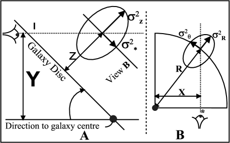
Figure 7: Dispersion projection in a plane parallel to galactic disc.

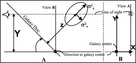
Figure 8: Projection of dispersions to the line-of-sight.

Second, we must project dispersions $\sigma^{2}_{z}$ and $\sigma^{2}_{\ast}$ to the line-of-sight. Designating $\Theta$ as the angle between the line-of-sight and the galactic disc, the line-of-sight dispersion $\sigma^{2}_{l}$ is

$$\sigma^{2}_{l}=\sigma^{2}_{\ast}\cos^{2}\Theta+\sigma^{2}_{z}\sin^{2}\Theta.$$ (29)

To compare the calculated dispersions with the measured data, we must calculate averaged along the line-of-sight dispersion. Integrating dispersions along the line-of-sight we may write

$$\sigma^{2}_{int}(X,Y)=\frac{1}{L(X,Y)}\int\limits^{\infty}_{-\infty}l(R,z)\sigma^{2}_{l}(R,z)\mathrm{d}l,$$ (30)

where $l(R,z)$ denotes galactic spatial luminosity density, and $L(X,Y)$ is the surface luminosity density profile (please note that integration $\mathrm{d}l$ means integration along the line-of-sight). Changing variables in the integral to have integration along the radius, we obtain

$$\sigma^{2}_{int}(X,Y)=\frac{1}{L(X,Y)}\int\limits^{\infty}_{X}\Psi\frac{R}{\cos{\Theta}\sqrt{R^{2}-X^{2}}}\mathrm{d}R,$$ (31)

where

$$\Psi\equiv l(R,z_{1})\sigma^{2}_{l}(R,z_{1})+l(R,z_{2})\sigma^{2}_{l}(R,z_{2}),$$ (32)

$$z_{1,2}=\left(\frac{Y}{\sin{\Theta}}\pm\sqrt{R^{2}-X^{2}}\right)\tan{\Theta}.$$ (33)

Equation (31) gives the line-of-sight dispersion for one galactic component. As in our model we have several components, we must sum over all components considering the luminosity distribution profile

$$\sigma_{\rm obs}(X,Y)=\left\{\frac{\sum\limits_{i}\left[L_{i}(X,Y)\left(\sigma^{2}_{int}(X,Y)\right)_{i}\right]}{\sum\limits_{i}L_{i}(X,Y)}\right\}^{1/2},$$ (34)

where $i$ denotes the subsystem and the summation is taken over all subsystems.

5 Velocity dispersion profiles of NGC 4594

In the present section we apply the above constructed model to a concrete galaxy. We selected the Sa galaxy NGC 4594 having enough observational data to construct a detailed mass distribution model. The velocity dispersions for NGC 4594 have been measured also along several slit positions outside of the galactic disc.

To avoid calculation errors, we first made several tests: we calculated dispersions for several simple density distribution profiles, varied the viewing angle between the disc and the line-of-sight, varied density distribution parameters. All test results were in accordance with our physical expectations.

In velocity dispersion calculations all the luminosity distribution model parameters derived in Section 3 will be handled as fixed. The visible part of the galaxy is given as a superposition of the nucleus, the bulge, the disc and the metal-poor halo. The spatial luminosity and mass density distributions of each visible component are consistent, i.e. their mass density distribution is given by

$$\rho(a)=\rho(0)\exp[-(a/(ka_{0}))^{1/N}],$$ (35)

where $\rho(0)=l(0)M/L=hM/(4\pi qa_{0}^{3})$ is the central mass density and $M$ is the component mass. For designations see Eq. (1).

In the case of mass distribution models, a DM component must be added to visible components. The DM distribution is represented by a spherical isothermal law

$$\rho(a)=\cases{\rho(0)\{[1+({a\over a_{c}})^{2}]^{-1}-[1+({a^{0}\over a_{c}})^{2}]^{-1}\}&$a\leq a^{0}$\cr 0&$a>a^{0}$.\cr}$$ (36)

Here $a^{0}$ is the outer cutoff radius of the isothermal sphere, $a_{c}=ka_{0}$.

Our model includes an additional unknown value – velocity ellipsoid orientation. We have to find the best solution to $z_{0}$, when fitting the model to the measured dispersions.

Figure 9 gives the shape and orientation of the velocity dispersion ellipsoid in the galactic meridional ($R,z$) plane.

Figure 9: Orientation of the calculated velocity dispersion ellipsoids in galactic meridional plane.

Figure 10: Line-of-sight velocity dispersions of NGC 4594 along and parallel to major axis. Solid line – calculated model dispersions, filled circles – observations.

In Figure 10 calculated line-of-sight dispersions along and parallel to galactic major axis are given. In Figure 11 calculated line-of-sight dispersions parallel to the minor axis are given.

Figure 11: Line-of-sight velocity dispersions of NGC 4594 parallel to the minor axis. Solid line – calculated model dispersions, filled circles – observations.

It is seen that moving further off from the galactic disc, the results become a little different from the data observed. One reason may be that we could not find an appropriate solution for $z_{0}$. It is possible to fit the data far from the galactic plane with appropriate selection of $z_{0}$ but in this case the fit with dispersions along the major axis is not so good. As a result, the figures present the best compromise solution we could find.

In addition we must take into account the observed average velocity dispersion of GCs $\sigma_{\mathrm{GC}}=255~{}\mathrm{km~{}s^{-1}}$. This value is clearly higher than the above mentioned last points in stellar dispersion curve $\sim 160-180~{}\mathrm{km~{}s^{-1}}$ (Fig. 11). All these dispersions correspond to a region where DM takes effect. For this reason we think that the mean velocity dispersion of GCs and and stellar velocity dispersions far outside of galactic plane can be fitted consistently by introducing a flattened DM halo density distribution. This kind of models have not yet been constructed by us within the present algorithm.

Figure 12 gives the calculated velocity dispersion in the $Rz$-plane illustrating the behavior of dispersions.

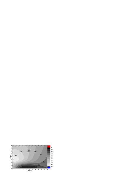
Figure 12: Projected line-of-sight dispersions (in $\mathrm{km~{}s^{-1}}$) in galactic meridional plane.

Table 2: Calculated model parameters.

Popul.	$M$	$a_{0}$	$q$	$N$	$k$	$h$	$\beta$	$L_{B}$	$L_{V}$	$L_{R}$	$L_{I}$
Nucleusa	0.001	0.0015	0.99	3.0	0.00297	314.3		3.9E-4
Bulge	3.4	0.28	0.54	2.1	0.03539	44.51	0.7	0.34	0.48	0.56	0.92
Halo	7.4	11.0	0.75	4.0	1.465E-4	2807.	0.3	3.2		4.4
Disc	12.0	3.4	0.25	0.78	0.7429	2.607	0.88	1.6	2.3	2.45	5.0
Dark matter	180	40.0	1.0		0.1512	14.82

• Masses and luminosities are in units of $10^{10}\mathrm{M_{\sun}}$ and $10^{10}\mathrm{L_{\sun}}$; components radii are in kpc.
  

• A point mass $10^{9}\mathrm{M_{\sun}}$ have been added to the center of the galaxy.

6 Discussion

In the present paper we developed an algorithm, allowing to construct a self-consistent mass and light distribution model and to calculate projected line-of-sight velocity dispersions outside galactic plane. We assume velocity dispersion ellipsoids to be triaxial and thus the phase density is a function of three integrals of motion. The galactic plane may have an arbitrary angle with respect to the plane of the sky. The developed algorithm is applied to construct a mass and light distribution model of the Sa galaxy M 104. In the first stage a luminosity distribution model was constructed on the basis of the surface brightness distribution. The inclination angle of the galaxy is known and the spatial luminosity distribution can be calculated directly with deprojection. Using the surface brightness distribution in $BVRI$ colours and along the major and minor axis, we assume that our components represent real stellar populations and determine their main structure parameters. In the second stage, the Jeans equations are solved and the line-of-sight velocity dispersions and the stellar rotation curve are calculated. Observations of velocity dispersions outside the apparent galactic major axis allow to determine the velocity ellipsoid orientation, anisotropy and to constrain DM halo parameters.

The total luminosity of the galaxy M 104 resulting from the best-fitting model is $L_{B}=(5.1\pm 0.6)\cdot 10^{10}\mathrm{L_{\sun}}$, $L_{R}=(7.4\pm 0.7)\cdot 10^{10}\mathrm{L_{\sun}}$. The total mass of the visible matter is $M_{\mathrm{vis}}=(22.9\pm 3.2)\cdot 10^{10}\mathrm{M_{\sun}}$, giving the mean mass-to-light ratio of the visible matter $M/L_{B}=4.5\pm 1.2~{}\mathrm{M_{\sun}L_{\sun}^{-1}}$, $M/L_{R}=3.1\pm 0.7~{}\mathrm{M_{\sun}L_{\sun}^{-1}}$. The surface brightness distributions in $V$ and $I$ have not sufficient extent to determine the luminosities of the stellar halo and we do not either give galactic total luminosities in these colours and corresponding $M/L$ ratios. Calculated from the model, the $L_{B}$ coincides well with the total absolute magnitude $M_{B}=-21.3$ ($=5.2\cdot 10^{10}~{}\mathrm{L_{\odot}}$) obtained by Ford et al. (1996).

In our model, the mass of the disc is $M_{\rm disc}=12\cdot 10^{10}\mathrm{M_{\sun}}$. This coincides rather well with the disc mass $11.4\cdot 10^{10}\mathrm{M_{\sun}}$ calculated with the help of Toomre’s stability criterion by van den Burg & Shane (1986) and with the mass $9.6\cdot 10^{10}\mathrm{M_{\sun}}$ derived by Emsellem et al. (1994). On the other hand, Emsellem et al. (1994) derived for the bulge mass $>5\cdot 10^{11}\mathrm{M_{\sun}}$, giving $M_{\mathrm{disc}}/M_{\mathrm{bulge}}=0.2$. This is similar to the value 0.25 derived by Jarvis & Freeman (1985), but this is much less than $M_{\mathrm{disc}}/M_{\mathrm{spher}}=1.1$ resulting from our model. An explanation may be that in the models by Emsellem et al. (1994) and Jarvis & Freeman (1985) no DM halo was included and hence the extended bulge mass is higher.

In our model, the disc is rather thick ($q=0.25$). However, disc thickness can be easily reduced to $q=0.15-0.2$ when taking the galactic inclination angle instead of $\delta=84\degr$ to be 83–82$\degr$. Other parameters remain nearly unchanged. At present this was not done.

Derived in the present model bulge parameters can be used to compare them with the results of chemical evolution models. Our model gives $M/L_{V}=7.1\pm 1.4~{}\mathrm{M_{\sun}L_{\sun}^{-1}}$ and $(B-V)=1.06$ for the bulge. Comparing spectral line intensities with chemical evolution models, Vazdekis et al. (1997) obtained for the bulge region the metallicity $Z=0.03$ and the age 11 Gyrs. According to Bruzual & Charlot (2003), these parameters give $M/L_{V}=7-8~{}\mathrm{M_{\sun}L_{\sun}^{-1}}$ and $(B-V)=1.06-1.08$ for simple stellar population (SSP) models. Bulge parameters from our dynamical model agree well with these values and suggest that our model is realistic.

In our calculations, we corrected luminosities from the absorption in the Milky Way only and did not take into account the inner absorption in M 104. According to Emsellem et al. (1996), absorption in the centre may be at least $A_{V}\sim 0.13$ mag and thus $M/L_{V}=6.3$ for the bulge. This is slightly too small when compared with the Bruzual & Charlot (2003) SSP models. However, decreasing the bulge age to 10.5 Gyrs allows to fit the results.

Rather sophisticated models of M 104 have been constructed by Emsellem et al. (1994, 1996) and Emsellem & Ferruit (2000). Due to our different approaches, it is difficult to compare our components and their parameters with those of Emsellem et al. (1994, 1996). On the basis of the data used by us, we had no reason to add an additional inner disc or a bar to the bulge region. However, we did not analyse $I$ and $H$ colours and ionized gas kinematics in inner regions as it was done by Emsellem & Ferruit (2000). Modelling of gas kinematics in central regions is beyond the scope of the present paper as gas is not collision-free.

On the basis of velocity dispersion observations only along the major axis it is difficult to decide about the presence of the DM even when dispersions extend up to 2–3 $\mathrm{R_{e}}$ (Samurović & Danziger, 2005). In the case of M 104, additional dispersion measurements can be used. Velocity dispersions in the case of the slit positioned parallel and perpendicular to the galactic major axis, have been measured by Kormendy & Illingworth (1982). The calculated mass distribution model describes rather well the observed stellar rotation curve and line-of-sight velocity dispersions. Only the two last measured points at a cut 50 arcsec perpendicular to the major axis deviate rather significantly when compared to the model. On the other hand, in addition to stellar velocity dispersion measurements, the mean line-of-sight velocity dispersion of the GC subsystem $\sigma=255~{}\mathrm{km~{}s^{-1}}$ was measured by Bridges et al. (1997). This corresponds to GCs at average distances 5–10 kpc from the galactic center and is in rather good agreement with the dispersions calculated from the model.

In the best-fitting model the DM halo harmonic mean radius $a_{0}=40$ kpc and $M=1.8\cdot 10^{12}{\rm M_{\sun}}$ giving slightly falling rotation curve in outer parts of the galaxy (Fig. 5). The central density of the DM halo in our model is $\rho(0)=0.033~{}\mathrm{M_{\sun}pc^{-3}}$, being also slightly less than it was derived for distant ($z\sim~{}0.9$) galaxies ($\rho(0)=0.012-0.028~{}\mathrm{M_{\sun}pc^{-3}}$, Tamm & Tenjes, 2005). On the other hand, the result fits with the limits derived by Boriello & Salucci (2001) for local galaxies $\rho(0)=0.015-0.050~{}\mathrm{M_{\sun}pc^{-3}}$.

An essential parameter in mass distribution determination is the inclination of the velocity dispersion ellipsoid with respect to the galactic plane (see e.g. Kuijken & Gilmore, 1989; Merrifield, 1991). Velocity dispersion ellipsoid inclinations calculated in the present paper are moderate, being $\leq 30\degr$. In a sense, our approach to the third integral of stellar motion is similar to that by Kent & de Zeeuw (1991) – the local Stäckel fit. In their modelling of the local Milky Way structure, they derived that at $0<z<600$ pc and $6.8<R<8.8$ kpc, the inclination of the velocity dispersion ellipsoid is less than $z/R$, and they studied the corresponding correction in detail. In our model, in the same distance regions (although the Milky Way and M 104 are not very similar objects), inclination correction values are slightly smaller. Variations of the corrections with $R$ and $z$ are qualitatively similar. The largest difference is the variation of the correction value with $z$, for which Kent & de Zeeuw (1991) obtained an increase by 0.1, when moving from $z=0$ to $z=0.6$ kpc, but in our model, corresponding increase was only by 0.01. In our model, a significant increase of the ellipsoid inclination angle begins at larger $z$, which can be explained by higher thickness of the disc component of M 104 ($q=0.25$). In a following paper we intend to construct similar models for other galaxies with velocity dispersion measurements outside the galactic major axis. This may lead to more firm conclusions about the inclination of velocity dispersion ellipsoids outside the galactic plane.

Ratios of the line-of-sight velocity dispersions are given in Fig. 13. It is seen that velocity dispersion ellipsoids are quite elongated – anisotropies in the symmetry plane at outer parts of the galaxy are $<0.5$.

Figure 13: Dispersion ratios in galactic meridional plane. Coordinate $z$ is in kpc.

Modelling the disc Sb galaxy NGC 288 within a constant velocity ellipsoid inclination approximation, Gerssen, Kuijken & Merrifield (1997) estimated that the dispersion ratio $\sigma_{z}/\sigma_{R}=0.70$. Within epicycle approximation Westfall et al. (2005) derived for Sb galaxy NGC 3982 the dispersion anisotropy $\sigma_{z}/\sigma_{R}=0.73$. These two galaxies are morphologically close to the Sa galaxy modelled in the present paper, and it is seen that dispersion ratios are more anisotropic in our case. In general, a radially elongated dispersion ellipsoid is rather common (Shapiro, Gerssen & van der Marel, 2003). On the other hand, there are exceptions – galaxy NGC 3949 (Westfall et al. (2005) has the dispersion ratio $\sigma_{z}/\sigma_{R}=1.18$).

By using the quadratic programming method (Dejonghe, 1989), the distribution function within the three-integral approximation has been numerically calculated for the S0 galaxy NGC 3115 by Emsellem, Dejonghe & Bacon (1999). Assuming some similarity between S0 and Sa galaxies, it is interesting to compare the derived velocity dispersion behaviour outside the galactic plane. Although detailed comparison is difficult a similar structure of isocurves is seen. But the results disagree in values of $\sigma_{z}/\sigma_{R}$. Our ratios are radially elongated, the ratios by Emsellem et al. (1999) are vertically elongated. Qualitatively this is in agreement with the general trend that galaxies of earlier morphological type have larger $\sigma_{z}/\sigma_{R}$ ratio (Shapiro et al., 2003). At larger $R$, the dispersion ratio $\sigma_{z}/\sigma_{R}$ decreases. This is in agreement with the decrease of dispersion ratios due to the decrease of the role of interactions with molecular clouds at greater galactocentric distances (see Jenkins & Binney, 1990). The use of this explanation in the case of gas-poor S0 galaxies is not clear. At greater distances $z$ both our and Emsellem et al. (1999) dispersion ellipsoids become more spherical.

By using the Schwarzschild method, dispersion ratios for E5–6 galaxy NGC 3377 have been calculated by Copin, Cretton & Emsellem (2004). Taking into account relation between spherical and cylindrical coordinates, the behaviour of the dispersion ratios as a function of $R$ and $z$ near the galactic plane is in approximate accordance (dispersion ratios by Copin et al. (2004) are slightly more spherical). Rotational properties of elliptical and Sa galaxies are too different to compare the ratios $\sigma_{\theta}/\sigma_{R}$. Unfortunately, it is not possible to compare also orientations of velocity dispersion ellipsoids.

References

- Amendt & Cudderford (1991) Amendt P., Cudderford P., 1991, ApJ, 368, 79
- An & Evans (2006) An J.H., Evans N.W., 2006, AJ, 131, 782
- Bajaja et al. (1984) Bajaja E., van der Burg G., Faber S.M., Gallagher J.S., Knapp G.R., Shane W.W., 1984, A&A, 141, 309
- Beck et al. (1984) Beck R., Dettmar R.J., Wielebinski R., Loiseau N., Martin C., Schnur G.F.O., 1984, ESO Messenger, Nr 36, 29
- Bertin et al. (1997) Bertin G., Leeuwin F., Pegoraro F., Pubini F., 1997, A&A, 321, 703
- Binney & Mamon (1982) Binney J., Mamon G.A., 1982, MNRAS, 200, 361
- Binney & Tremaine (1987) Binney J., Tremaine S., 1987, Galactic Dynamics. Princeton Univ. Press, Princeton, NJ
- Binney et al. (1990) Binney J.J., Davies R.L., Illingworth G.D., 1990, ApJ, 361, 78
- Boriello & Salucci (2001) Boriello A., Salucci P., 2001, MNRAS, 323, 285
- Boroson (1981) Boroson T., 1981, ApJS, 46, 177
- Bridges & Hanes (1992) Bridges T.J., Hanes D.A., 1992, AJ, 103, 800
- Bridges et al. (1997) Bridges T.J., Ashman K.M., Zepf S.E., Carter D., Hanes D.A., Sharples R.M., Kavelaars J.J., 1997, MNRAS, 284, 376
- Bruzual & Charlot (2003) Bruzual G., Charlot S., 2003, MNRAS, 344, 1000
- Burkhead (1979) Burkhead M.S., 1979, in Photometry, kinematics and dynamics of galaxies; ed. D.S. Evans, Univ Texas, Austin, p. 143
- Burkhead (1986) Burkhead M.S., 1986, AJ, 91, 777
- Cappellari et al. (2002) Cappellari M., Verolme E.K., van der Marel R.P., Verdoes Kleijn G.A., Illingworth G.D., Franx M., Carollo C.M., de Zeeuw P.T., 2002, ApJ, 578, 787
- Carollo et al. (1995) Carollo C.M., de Zeeuw P.T., van der Marel R.P., 1995, MNRAS, 276, 1131
- Carter & Jenkins (1993) Carter D., Jenkins C.R., 1993, MNRAS, 263, 1049
- Cinzano & van der Marel (1994) Cinzano P., van der Marel R.P., 1994, MNRAS, 270, 325
- Copin et al. (2004) Copin Y., Cretton N., Emsellem E., 2004, A&A, 415, 889
- Crane et al. (1993) Crane P. et al., 1993, ApJ, 417, 528
- Cretton et al. (1999) Cretton N., de Zeeuw P.T., van der Marel R.P., Rix H.-W., 1999, ApJS, 124, 383
- Dejonghe (1989) Dejonghe H., 1989, ApJ, 343, 113
- de Bruijne et al. (1996) de Bruijne J.H.J., van der Marel R.P., de Zeeuw P.T., 1996, MNRAS, 282, 909
- Dehnen (1995) Dehnen W., 1995, MNRAS, 274, 919
- Dehnen & Gerhard (1993) Dehnen W., Gerhard O.E., 1993, MNRAS, 261, 311
- Dejonghe & de Zeeuw (1988) Dejonghe H., de Zeeuw T., 1988, ApJ, 333, 90
- de Zeeuw et al. (1996) de Zeeuw P.T., Evans N.W., Schwarzschild M., 1996, MNRAS, 280, 903
- Dutton et al. (2005) Dutton A.A., Courteau S., de Jong R., Carignan C., 2005, ApJ, 619, 218
- Einasto (1970) Einasto J., 1970, Afz, 6, 149
- Einasto & Haud (1989) Einasto J., Haud U., 1989, A&A, 223, 89
- Einasto & Tenjes (1999) Einasto J., Tenjes P., 1999, in The stellar content of Local Group galaxies, IAU Symp. 192. ASP, San Francisco, 341
- Emsellem & Ferruit (2000) Emsellem E., Ferruit P., 2000, A&A, 357, 111
- Emsellem et al. (1994) Emsellem E., Monnet G., Bacon R., Nieto J.-L., 1994, A&A, 285, 739
- Emsellem et al. (1996) Emsellem E., Bacon R., Monnet G., Poullain P., 1996, A&A, 312, 777
- Emsellem et al. (1999) Emsellem E., Dejonghe H., Bacon R., 1999, MNRAS, 303, 495
- Evans (1993) Evans N.W., 1993, MNRAS, 260, 191
- Fisher et al. (1994) Fisher D., Illingworth G., Franx M., 1994, AJ, 107, 160
- Ford et al. (1996) Ford H.C., Hui X., Ciardullo R., Freeman K.C., 1996, ApJ, 458, 455
- Frei & Gunn (1994) Frei Z., Gunn J.E., 1994, AJ, 108, 1476
- Gentile et al. (2004) Gentile G., Salucci P., Klein U., Vergani D., Kalberla P., 2004, MNRAS, 351, 903
- Gerhard (1991) Gerhard O.E., 1991, MNRAS, 250, 812
- Gerssen et al. (1997) Gerssen J., Kuijken K., Merrifield M., 1997, MNRAS, 288, 618
- Hamabe & Okamura (1982) Hamabe M., Okamura S., 1982, Ann Tokyo Astron Obs, Sec Ser, 18, 191
- Hes & Peletier (1993) Hes R., Peletier R.F., 1993, A&A, 268, 539
- Illiingworth & Schechter (1982) Illingworth G., Schechter P.L., 1982, ApJ, 256, 481
- Jarvis & Freeman (1985) Jarvis B.J., Freeman K.C., 1985, ApJ, 295, 324
- Jenkins & Binney (1990) Jenkins A., Binney J., 1990, MNRAS, 245, 305
- Kent (1988) Kent S.M., 1988, AJ, 96, 514
- Kent & de Zeeuw (1991) Kent S.M., de Zeeuw T., 1991, AJ, 102, 1994
- (51) Khairul Alam S. M., Bullock J. S., Weinberg D. H., 2002, ApJ, 572, 34
- Kormendy (1988) Kormendy J., 1988, ApJ, 335, 40
- Kormendy & Illingworth (1982) Kormendy J., Illingworth G., 1982, ApJ, 256, 460
- Kormendy et al. (1996) Kormendy J. et al., 1996, ApJ, 473, L91
- Krajnović et al. (2005) Krajnocić D., Cappellari M., Emsellem E., McDermid R.M., de Zeeuw P.T., 2005, MNRAS, 357, 1113
- Kuijken & Gilmore (1989) Kuijken K., Gilmore G., 1989, MNRAS, 239, 605
- Kuzmin (1953) Kuzmin G.G., 1953, Tartu Astron. Obs. Publ., 32, 332
- Kuzmin (1961) Kuzmin G.G., 1961, Tartu Astron. Obs. Publ., 33, 351
- Kuzmin (1962) Kuzmin G.G., 1962, Bull. Abastumani Astrophys. Obs., 27, 89 (1963, Tartu Astrophys. Obs. Teated, 6, 16)
- Landau & Livshits (1976) Landau L.D., Livshits E.M., 1976, Mechanics (Course of Theor Phys), Butterworth-Heinemann, 3rd Ed.
- Larsen et al. (2001) Larsen S.S., Forbes D.A., Brodie J.P., 2001, MNRAS, 327, 1116
- Mazure & Capelato (2002) Mazure A., Capelato H.V., 2002, A&A, 383, 384
- Merrifield (1991) Merrifield M.R., 1991, AJ, 102, 1335
- Merritt (1985) Merritt D., 1985, AJ, 90, 1027
- Merritt (1996) Merritt D., 1996, AJ, 112, 1085
- Navarro & Steinmetz (2000) Navarro J.F., Steinmetz M., 2000, ApJ, 528, 607
- Rhode & Zepf (2004) Rhode K.L., Zepf S.E., 2004, AJ, 127, 302
- Rix et al. (1997) Rix H.-W., de Zeeuw P.T., Cretton N., van der Marel R.P., Carollo C.M., 1997, ApJ, 488, 702
- Rubin et al. (1985) Rubin V.C., Burstein D., Ford Jr W.K., Thonnard N., 1985, ApJ, 289, 81
- Samurović & Danziger (2005) Samurović S., Danziger I.J., 2005, MNRAS, 363, 769
- Schlegel et al. (1998) Schlegel D.J., Finkbeier D.P., Davis M., 1998, ApJ, 500, 525
- Schwarzschild (1979) Schwarzschild M., 1979, ApJ, 232, 236
- Schweizer (1978) Schweizer F., 1978, ApJ, 220, 98
- Sérsic (1968) Sérsic J.L., 1968, Atlas de Galaxies Australes, Observatorio Astronomico, Cordoba, Argentina
- Shapiro et al. (2003) Shapiro K.L., Gerssen J., van der Marel R.P., 2003, AJ, 126, 2707
- Spinrad et al. (1978) Spinrad H., Ostriker J.P., Stone R.P.S., Chiu L.-T.G., Bruzual G.A., 1978, ApJ, 225, 56
- Statler & Smecker-Hane (1999) Statler T.S., Smecker-Hane T., 1999, AJ, 117, 839
- Tamm & Tenjes (2005) Tamm A., Tenjes P., 2005, A&A, 433, 31
- Tenjes et al. (1994) Tenjes P., Haud U., Einasto J., 1994, A&A, 286, 753
- Tenjes et al. (1998) Tenjes P., Haud U., Einasto J., 1998, A&A, 335, 449
- Tonry et al. (2001) Tonry J.L., Dressler A., Blakeslee J.P., Ajhar E.A., Fletcher A.B., Luppino G.A., Metzger M.R., Moore C.B., 2001, ApJ, 546, 681
- Tremaine et al. (1994) Tremaine S., Richstone D.O., Byun Y.-I., Dressler A., Faber S.M., Grillmair C., Kormendy J., Lauer T.R., 1994, AJ, 107, 634
- van den Burg & Shane (1986) van den Burg G., Shane W.W., 1986, A&A, 168, 49
- van der Marel et al. (1990) van der Marel R.P., Binney J., Davies R.L., 1990, MNRAS, 245, 582
- van der Marel et al. (1994) van der Marel R.P., Rix H.-W., Carter D., Franx M., White S.D.M., de Zeeuw P.T., 1994, MNRAS, 268, 521
- van der Marel et al. (1998) van der Marel R.P., Cretton N., de Zeeuw P.T., Rix H.-W., 1998, ApJ, 493, 613
- Vazdekis et al. (1997) Vazdekis A., Peletier R.F., Beckman J.E., Casuso E., 1997, ApJS, 111, 203
- Verolme et al. (2002) Verolme E.K. et al., 2002, MNRAS, 335, 517
- Westfall et al. (2005) Westfall K.B., Bershady M.A., Verheijen M.A.W., Andersen D.R., Swaters R.A., 2005, in Islandic universes: structure and evolution of disc galaxies, Netherlands, July 3–8, 2005 (astro-ph/0508552)